Control of spin relaxation in semiconductor double quantum dots

Abstract

We propose a scheme to manipulate the spin relaxation in vertically coupled semiconductor double quantum dots. Up to twelve orders of magnitude variation of the spin relaxation time can be achieved by a small gate voltage applied vertically on the double dot. Different effects such as the dot size, barrier height, inter-dot distance, and magnetic field on the spin relaxation are investigated in detail. The condition to achieve a large variation is discussed.

Spin related phenomena in semiconductor nanostructures have attracted much interest recently due to the fast growing field of spintronics Awschalom . Among different structures, quantum dots (QDs) have caused a lot of attention as they provide a versatile system to manipulate the spin and/or electronic states Hans . Many proposals of spin qubits, spin filters, spin pumps and spin quantum gates are proposed and/or demonstrated based on different kinds of QDs Hans ; Barenco ; Loss ; Burkard ; das ; Folk ; Aono ; Recher ; Ernesto ; Romo . Manipulation and understanding of the spin coherence in QDs are of great importance in the design and the operation of these spin devices. There are many theoretical and experimental investigations on the spin relaxation in single QDs Alexander ; Governale ; Woods ; Cheng ; Tsitsishvili ; Golovach ; hanson , double QDs johnson ; Peter and quasi-one-dimension coupled QDs Tamborenea due to the Dresselhaus or Rashba spin-orbit couplings Dresselhaus ; Yu . In this paper, we propose a feasible and convenient way to manipulate the spin relaxation in double QDs by a small gate voltage. We show that up to twelve orders of magnitude variation of the longitudinal spin relaxation time (SRT) can be tuned in such a system.

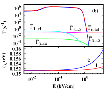
Figure 1: (Color online) (a) SRT vs. the electric field. Solid curve: perturbation result; Dotted curve: exact diagonalization result; Inset: Schematic of the potential along the vertical ($z$) direction. (b) Upper panel: Weighted scattering rates $\bar{\Gamma}_{i\to j}$ between different energy levels (from “spin-up” to “spin-down”) vs. the electric field. $\bar{\Gamma}_{\mbox{total}}$ is the total weighted scattering rate from the “spin-up” to the ”spin-down” states. Lower panel: Energy level $\varepsilon_{\lambda}$ of the $z$ direction of the double QD vs. the electric field.

We consider a single electron spin in two vertically coupled QDs. Each QD is confined by a parabolic potential $V_{c}({\bf r})=\frac{1}{2}m^{\ast}\omega_{0}^{2}{\bf r}^{2}$ (Therefore the effective dot diameter $d_{0}=\sqrt{\hbar\pi/m^{\ast}\omega_{0}}$) along the $x$-$y$ plane in a quantum well of width $d$ with its growth direction along the $z$-axis. A gate voltage $V_{d}$ together with a magnetic field $B$ are applied along the growth direction. A schematic of the potential of the coupled quantum wells is plotted in the inset of Fig. 1(a) and the potential is given bycomment

$$V_{z}(z)=\begin{cases}eEz+\frac{1}{2}eV_{d},&\frac{1}{2}a<|z|<\frac{1}{2}a+d\\ eEz+\frac{1}{2}eV_{d}+V_{0},&|z|\leqslant\frac{1}{2}a\\ \infty,&\mbox{otherwise}\end{cases}$$ (1)

in which $V_{0}$ represents the barrier height between the two coupled QDs, $a$ is the barrier width and $E=V_{d}/(a+2d)$ denotes the electric field due to the gate voltage. The origin of the $z$-axis is chosen to be the center of the barrier between the two QDs. By solving the Schrödinger equations along the $z$-axis ${d^{2}\psi_{z}}/{d\xi_{i}^{2}}-\xi_{i}\psi_{z}=0$ with $\xi_{1}=2^{1/3}(\frac{m^{\ast}}{\hbar^{2}e^{2}E^{2}})^{1/3}(eEz-\varepsilon+eV_{d}/2)$ for $\frac{1}{2}a<|z|<\frac{1}{2}a+d$ and $\xi_{2}=2^{1/3}(\frac{m^{\ast}}{\hbar^{2}e^{2}E^{2}})^{1/3}(eEz-\varepsilon+eV_{d}/2+V_{0})$ for $|z|\leqslant\frac{1}{2}a$, one obtains the wave function:

$$\psi_{z}(z)=\begin{cases}A_{1}\mbox{Ai}(\xi_{1})+A_{2}\mbox{Bi}(\xi_{1}),&-(\frac{a}{2}+d)<z<-\frac{a}{2}\\ B_{1}\mbox{Ai}(\xi_{2})+B_{2}\mbox{Bi}(\xi_{2}),&|z|\leqslant\frac{1}{2}a\\ C_{1}\mbox{Ai}(\xi_{1})+C_{2}\mbox{Bi}(\xi_{1}),&\frac{a}{2}<z<\frac{a}{2}+d\\ \end{cases}$$ (2)

in which Ai and Bi are the Airy functions. The coefficients together with the eigenenergy $\varepsilon_{\lambda}$ can be obtained from the boundary conditions $\psi_{z\lambda}(z=\pm(a/2+d))=0$, the continuity conditions at $z=\pm\frac{1}{2}a$ and the condition of normalization $\int\psi_{z\lambda}^{\ast}(z)\psi_{z\lambda}(z)dz=1$. The electron Hamiltonian in the $x$-$y$ plane is $H_{e}=H_{0}+H_{so}$, where $H_{0}=(P_{x}^{2}+P_{y}^{2})/(2m^{\ast})+V_{c}({\bf r})+H_{B}$ is electron Hamiltonian without the spin-orbit interaction, in which ${\bf P}\equiv(P_{x},P_{y})=-i\hbar\nabla+(e/c)\bf{A}$ with ${\bf A}=(B/2)(-y,x)$ is the electron momentum operator. $m^{\ast}$ is the electron effective mass. $H_{B}=\frac{1}{2}g\mu_{B}B\sigma_{z}$ is the Zeeman energy with $\sigma_{z}$ denoting the Pauli matrix. $H_{so}=\frac{\gamma}{\hbar^{3}}\sum_{\lambda}\langle P_{z}^{2}\rangle_{\lambda}(-P_{x}\sigma_{x}+P_{y}\sigma_{y})$ is the Dresselhaus spin-orbit coupling Dresselhaus with $\langle P_{z}^{2}\rangle_{\lambda}\equiv-\hbar^{2}\int\psi_{z\lambda}^{\ast}(z)\partial^{2}/\partial z^{2}\psi_{z\lambda}(z)dz$ and $\gamma=27.5$ Å${}^{3}\cdot$eV Knap . For the small applied gate voltage, the Rashba spin-orbit coupling Yu is unimportant in this study flat . The eigenenergy of $H_{0}$ is $E_{nl\sigma}=\hbar\Omega(2n+|l|+1)-\hbar l\omega_{B}+\sigma E_{B}$, in which $\Omega=\sqrt{\omega_{0}^{2}+\omega_{B}^{2}}$, $\omega_{B}=eB/(2m^{\ast})$ and $E_{B}=\frac{1}{2}g\mu_{B}B$. The eigenfunction $\langle{\bf r}|nl\sigma\rangle=N_{n,l}(\alpha r)^{|l|}e^{-(\alpha r)^{2}}L_{n}^{|l|}((\alpha r)^{2})e^{il\theta}\chi_{\sigma}$ with $N_{n,l}=(\alpha^{2}n!/\pi(n+|l|)!)^{1/2}$ and $\alpha=\sqrt{m^{\ast}\Omega/\hbar}$. $L_{n}^{|l|}$ is the generalized Laguerre polynomial. $\chi_{\sigma}$ represents the eigenfunction of $\sigma_{z}$. In these equations $n=0,1,2,\cdots$, $l=0,\pm 1,\pm 2,\cdots$ and $\sigma=\pm 1$ are quantum numbers. From the eigenfunction of $H_{0}$, one can construct the wave function $|\Psi_{\ell}\rangle$ of $H_{e}$ by either the perturbation calculations Alexander ; Woods modified by the right energy corrections pointed out by Cheng et al. Cheng or the exact diagonalization approach.Cheng

The SRT $\tau$ is calculated from $\tau^{-1}=\sum_{if}f_{i}\Gamma_{i\to f}$ in which $f_{i}=C\exp[-E_{i}/(k_{B}T)]$ denotes the Maxwell distribution of the $i$-th level with $C$ standing for the normalization parameter and

$$\Gamma_{i\to f} = \frac{2\pi}{\hbar}\sum_{{\bf q}{\lambda_{1}}}|M_{{\bf q}{\lambda_{1}}}|^{2}|\langle f|e^{i{\bf q}\cdot{\bf r}}|i\rangle|^{2}\Big{[}\bar{n}_{{\bf q}{\lambda_{1}}}\delta(E_{f}-E_{i}$$ (3)

$$\mbox{}-\hbar\omega_{{\bf q}{\lambda_{1}}})+(\bar{n}_{{\bf q}{\lambda_{1}}}+1)\delta(E_{f}-E_{i}+\hbar\omega_{{\bf q}{\lambda_{1}}})\Big{]}$$

is the transition rate from the $i$-th level to the $f$-th one due to the electron-phonon scattering due to the deformation potential with $|M_{{\bf q}sl}|^{2}=\hbar\Xi^{2}q/2Dv_{sl}$ and the piezoelectric coupling for the longitudinal phonon mode with $|M_{{\bf q}pl}|^{2}=(32\hbar\pi^{2}e^{2}e_{14}^{2}/\kappa^{2}Dv_{sl})[(3q_{x}q_{y}q_{z})^{2}/q^{7}]$ and for the two transverse phonon modes with $\sum_{j=1,2}|M_{{\bf q}pt_{j}}|^{2}=(32\hbar\pi^{2}e^{2}e_{14}^{2}/\kappa^{2}Dv_{st}q^{5})[q_{x}^{2}q_{y}^{2}+q_{y}^{2}q_{z}^{2}+q_{z}^{2}q_{x}^{2}-(3q_{x}q_{y}q_{z})^{2}/q^{2}]$. $\bar{n}_{{\bf q}{\lambda_{1}}}$ represents the Bose distribution of phonon with mode ${\lambda_{1}}$ and momentum ${\bf q}$ at the temperature $T$. Here $\Xi=7$ eV stands for the acoustic deformation potential; $D=5.3\times 10^{3}$ kg/m³ is the GaAs volume density; $e_{14}=1.41\times 10^{9}$ V/m is the piezoelectric constant and $\kappa=12.9$ denotes the static dielectric constant. The acoustic phonon spectra are given by $\omega_{{\bf q}ql}=v_{sl}q$ for the longitudinal mode and $\omega_{{\bf q}pt}=v_{st}q$ for the transverse modes with $v_{sl}=5.29\times 10^{3}$ m/s and $v_{st}=2.48\times 10^{3}$ m/s being the corresponding sound velocities.

The states $i$ and $f$ in Eq. (3) are the eigenstates of the Hamiltonian $H_{e}$. In order to demonstrate the physics clearly, we first use the corrected perturbation method by Cheng et al. Cheng to study the SRT. For the double dot system, we need to include the lowest two energy levels of z direction which we label as $|1_{z}\rangle$ and $|2_{z}\rangle$ [Eq. (2)]. In $x$-$y$ plane, the lowest six energy levels of $H_{0}$ for each QD are considered, i.e., $|00+\rangle$, $|00-\rangle$, $|01+\rangle$, $|01-\rangle$, $|0-1+\rangle$, and $|0-1-\rangle$. The wave functions of the lowest four states of $H_{e}+\frac{P_{z}^{2}}{2m^{\ast}}+V_{z}$ constructed from these levels are therefore given by

$$|\Psi_{1}\rangle = |00+\rangle|1_{z}\rangle-{\cal B}_{1}|0-1-\rangle|1_{z}\rangle\ ,$$ (4)

$$|\Psi_{2}\rangle = |00-\rangle|1_{z}\rangle-{\cal A}_{1}|01+\rangle|1_{z}\rangle\ ,$$ (5)

$$|\Psi_{3}\rangle = |00+\rangle|2_{z}\rangle-{\cal B}_{2}|0-1-\rangle|2_{z}\rangle\,$$ (6)

$$|\Psi_{4}\rangle = |00-\rangle|2_{z}\rangle-{\cal A}_{2}|01+\rangle|2_{z}\rangle\ ,$$ (7)

with the corresponding energies being:

$$E_{1} = E_{00+,1}-|{\cal B}_{1}|^{2}(E_{0-1-,1}-E_{00+,1})\ ,$$ (8)

$$E_{2} = E_{00-,1}-|{\cal A}_{1}|^{2}(E_{01+,1}-E_{00-,1})\ ,$$ (9)

$$E_{3} = E_{00+,2}-|{\cal B}_{2}|^{2}(E_{0-1-,2}-E_{00+,2})\ ,$$ (10)

$$E_{4} = E_{00-,2}-|{\cal A}_{2}|^{2}(E_{01+,2}-E_{0-,2})\ .$$ (11)

In these equations $E_{nl\sigma,\lambda}=E_{nl\sigma}+\varepsilon_{\lambda}$; ${\cal B}_{\lambda}=i\alpha\gamma_{\lambda}^{\ast}(1-eB/(2\hbar\alpha^{2}))/(E_{0-1-,\lambda}-E_{00+,\lambda})$ and ${\cal A}_{\lambda}=i\alpha\gamma_{\lambda}^{\ast}(1+eB/(2\hbar\alpha^{2}))/(E_{01+,\lambda}-E_{00-,\lambda})$ with $\gamma_{\lambda}^{\ast}=\gamma\langle P_{z}^{2}\rangle_{\lambda}/\hbar^{2}$. $\lambda$($=1,2$) is the quantum number of $z$-axis. Now we calculate the spin-flip rates from the “spin-up” states $|\Psi_{2m-1}\rangle$ to the “spin-down” ones $|\Psi_{2m}\rangle$ ($m=1,2$) due to the electron-phonon scattering. There are nine spin-flip scattering rates. The scatting rate from the “spin-up” state $i$ to the “spin-down” one $f$ reads

$$\Gamma_{i\to f} = |{\cal A}_{f}-{\cal B}_{i}|^{2}\{n_{q}+[1+\mbox{sgn}(i-f)]/2\}q^{3}\int_{0}^{\pi/2}d\theta$$ (12)

$$\mbox{}\times\Big{[}C_{LD}q^{2}\sin^{3}\theta+C_{LP}q^{2}\sin^{7}\theta\cos^{2}\theta+C_{TP}\sin^{5}\theta$$

$$\mbox{}\times(\sin^{4}\theta+8\cos^{4}\theta)\Big{]}e^{-q^{2}\sin^{2}\theta/2}|I_{if}(q\cos\theta)|^{2}\ ,$$

in which $I_{if}(q_{z})=\langle\psi_{zi}|e^{iq_{z}z}|\psi_{zf}\rangle$ and $q=|E_{i}-E_{f}|/(\hbar v_{\lambda}\alpha)$. $C_{LD}=\Xi^{2}\alpha^{3}/(8\pi\hbar v_{sl}^{2}D)$, $C_{LP}=9e^{2}e_{14}^{2}\alpha\pi/(\hbar\kappa^{2}Dv_{sl}^{2})$ and $C_{TP}=\pi e^{2}e_{14}^{2}\alpha/(\hbar\kappa^{2}Dv_{st}^{2})$ in Eq. (12) are the coefficients from the electron-phonon scattering due to the deformation potential and due to the piezoelectric coupling for the longitudinal phonon mode and two transverse phonon modes respectively.

In Fig. 1 we plot the SRT of a typical double dot with $d_{0}=20$ nm, $a=10$ nm, $d=5$ nm, $V_{0}=0.4$ eV and $B=0.1$ T at $T=4$ K as a function of electric field $E$. The solid curve in Fig. 1(a) is the result from the perturbation approach. It is interesting to see that the SRT is increased about seven orders of magnitude when the electric field is tuned from $0.1$ kV/cm to $1.3$ kV/cm. The physics of such gate-voltage-induced dramatic change can be understood as follows: When the gate voltage is small, due to the large well height $V_{0}$ and/or large inter-dot distance $a$, the electron wavefunction (along the $z$-axis) of the lowest subband of each well is mostly localized in that well due to the high barrier between them and hence the difference of the lowest two energy levels is very small (about $10^{-4}$ eV). When a gate voltage is high enough, electron can tunnel through the barrier and the wavefunctions in the two wells get large overlap. Therefore the separation between the lowest two levels $\varepsilon_{1}$ and $\varepsilon_{2}$ increases. This can be seen from Fig. 1(b) where the energies of the lowest two levels along the z-axis $\varepsilon_{1}$ and $\varepsilon_{2}$ are plotted against electric field $E$. From Eqs. (8-11) one can see that the first two levels ($E_{1}$ and $E_{2}$) and the next two levels ($E_{3}$ and $E_{4}$) are mainly separated by the energy along the $z$-axis, i.e., $\varepsilon_{1}$ and $\varepsilon_{2}$. Such an increase makes the electron-phonon scattering more efficient when the energy difference $\varepsilon_{2}-\varepsilon_{1}$ is not too big. Therefore, by applying the gate voltage, one finds the SRT first decreases. Nevertheless, with the further increase of the gate voltage, half of the lowest four levels are quickly removed from the spin relaxation channel and the SRT is enhanced. As a result, there is a minimum of SRT with the gate voltage. This can be seen from the same figure where the weighted scattering rates ($\bar{\Gamma}_{i\to f}=f_{i}\Gamma_{i\to f}$) between different levels are plotted versus the electric field. The leading contribution to the total scattering rate comes from $\bar{\Gamma}_{3\to 2}$ at small field regime. When the electric field increases from $0.5$ kV/cm to $1.3$ kV/cm, $\bar{\Gamma}_{3\to 2}$ decreases rapidly due to the separation of $\varepsilon_{\lambda}$ with the electric field but $\bar{\Gamma}_{1\to 2}$ keeps almost unchanged as both levels $E_{1}$ and $E_{2}$ correspond to the same lowest level $\varepsilon_{1}$ along the $z$-axis. Finally for large field, $\bar{\Gamma}_{1\to 2}$ defines the total scattering rate. It is further noted that although we performed the average of the initial and the sum of the final states in calculating the SRT, the leading contribution comes from the scattering from $E_{3}$ to $E_{2}$ at low electric field and the scattering from $E_{1}$ to $E_{2}$ at large one.

The large variation of $\bar{\Gamma}_{3\to 2}$ around 1 kV/cm can be estimated as following: As the electron-phonon scattering due to the piezoelectric coupling of the two transverse phonon modes is at least one order of magnitude larger than the other modes, we only consider the third term in Eq. (12). From our calculation, $\varepsilon_{1}=(3.25\times 10^{-4}E/(\mbox{kV/cm})+0.15129)$ eV and $\varepsilon_{2}=(1.68\times 10^{-3}E/(\mbox{kV/cm})+0.1513)$ eV. The energy splitting between $E_{2}$ and $E_{3}$ can be approximated by $\varepsilon_{2}-\varepsilon_{1}$. Therefore $\Delta E_{23}=(1.36\times 10^{-3}E/(\mbox{kV/cm})+5\times 10^{-5})$ eV approximately and $q=\Delta E_{23}/(\hbar v_{st}\alpha)$. As the variation of $|I_{12}(q\cos\theta)|$ in Eq. (12) is within one order of magnitude, we approximately bring it out of the integral. Then the remaining integral $\int_{0}^{\pi/2}d\theta\sin^{5}\theta(\sin^{4}\theta+8\cos^{4}\theta)e^{-q^{2}\sin^{2}\theta/2}$ can be carried out analytically: $\frac{1}{2}B(\frac{1}{2};5)\Phi(5;\frac{11}{2};-q^{2}/2)+4B(\frac{5}{2},3)\Phi(3;\frac{11}{2};-q^{2}/2)$ with $B(\mu;\nu)$ and $\Phi(\alpha;\gamma;z)$ being the Beta function and the degenerate Hypergeometric function separately. When $E=0.1$ kV/cm, the value of the integral is $10^{-1}$ and when $E=1.3$ kV/cm, it becomes $10^{-6}$. Meanwhile, with the change of the electric field from 0.1 kV/cm to 1.3 kV/cm, although $q^{3}|{\cal A}_{f}-{\cal B}_{i}|^{2}$ is increased by one order of magnitude, $|I_{23}|^{2}$ is decreased by one order of magnitude and the distribution function $f_{3}$ is decreased by another two orders of magnitude. Therefore, $\bar{\Gamma}_{3\to 2}$ decreases about seven orders of magnitude when $E$ is tuned from 0.1 kV/cm to 1.3 kV/cm.

As pointed out by Cheng et al. Cheng and confirmed by Destefani and Ulloa sergio that due to the strong spin-orbit coupling, the perturbation approach is inadequate in describing the SRT even when the second-order energy corrections are included. Therefore, in Fig. 1(a) we further plot the SRT calculated from the exact diagonalization as dotted curve. Similar results are obtained although again the SRT from the exact diagonalization approach differs from the perturbation one.

Figure 2: SRT calculated from the exact diagonalization approach vs. the electric field at (a) different magnetic fields with $d_{0}=20$ nm and (b) QD diameters with $B=0.1$ T. In the calculation $a=10$ nm, $d=5$ nm, $d_{0}=20$ nm, $V_{0}=0.4$ eV and $T=4$ K.

Now we investigate the magnetic field and dot size dependence of the SRT in Fig. 2(a) and (b) by exact diagonalization approach. Again one observes a dramatic increase of the SRT by tuning the electric field up to a certain value and then the SRT is insensitive to the electric field. For small dot size ($d_{0}=10$ nm), one even observes a twelve orders of magnitude change of the SRT by tuning the gate electric field to 2.6 kV/cm. The dramatic variation of the SRT has been explained above. Now we discuss why the SRT decreases with magnetic field and dot size observed in Fig. 2 in the electric-field-insensitive part. From Fig. 1(b) one finds $\bar{\Gamma}_{1\to 2}$ is the leading contribution to the total scattering rate in this part. The energy splitting between the first and the second levels $\Delta E_{12}\propto B$. As $\Delta E_{12}$ is about $10^{-5}$ eV, $n_{q}\simeq k_{B}T/\Delta E_{12}$ and $n_{q}q^{3}\propto(\Delta E_{12})^{2}$. Moreover $|{\cal A}_{1}-{\cal B}_{1}|^{2}=(\alpha\gamma_{1}^{\ast}4E_{B}\omega_{B})^{2}/(\hbar^{2}\Omega\omega_{0}^{2})^{2}\propto B^{4}$ proximately. As a result, the coefficient before the integral of the electron-transverse phonon scattering due to the piezoelectric coupling is proportion to $B^{6}$. Although the integral has a marginal decrease with $B$, $\bar{\Gamma}_{1\to 2}$ still increases with $B$. Similarly, one can explain the change of the SRT with the dot diameter $d_{0}$.

Figure 3: SRT calculated from the exact diagonalization approach vs. the electric field at (a) different barrier heights $V_{0}$ with the barrier width $a=10$ nm and (b) different barrier widthes $a$ with $V_{0}=0.4$ nm. In the calculation, $d=5$ nm, $d_{0}=20$ nm and $B=0.1$ T. $T=4$ K.

It is noted that in order to obtain the large variation of the SRT by a gate voltage, it is important that the barrier between the QDs should be large enough so that without a gate voltage, the two dots are decoupled (and there is no energy splitting along the $z$-axis). This can be clearly seen from Fig. 3: With the decrease of the barrier height $V_{0}$ or the inter-dot distance $a$, the tunability of the SRT by the gate voltage decreases.

Figure 4: SRT calculated from the exact diagonalization approach vs. the electric field at different inter-dot distance $a$ with low barrier height $V_{0}=0.05$ eV. In the calculation, $d=5$ nm, $d_{0}=20$ nm, $B=0.1$ T and $T=4$ K.

The double dot system proposed in our scheme can be easily realized with the current technology.Hatano ; Austing Nevertheless, it is not essential to use such a high barrier height system to obtain the large spin manipulation. For ordinary barrier height widely used in the experiment (which is about one order of magnitude lower than $V_{0}$ used above), one can still achieve the similar manipulation by increasing the distance $a$ between the two QDs as shown in Fig. 4 where the barrier height $V_{0}=0.05$ eV. One finds that for small $V_{0}$, if the barrier width $d$ is large enough, one can still get the large change of SRT. Especially, in the case of $a=30$ nm, eleven orders of magnitude change of SRT is obtained by a small gate field.

In conclusion, we have proposed a feasible scheme to manipulate the spin relaxation in GaAs vertical double DQs by a small gate voltage. The SRT calculated can be tuned up to twelve orders of magnitude by an electric field from the gate voltage less than 3 kV/cm. This provides a unique way to control the spin relaxation and to make spin-based logical gates. The conditions to realize such a large tunability are addressed. The double dot system proposed in our scheme can be easily realized in the experiment. Finally the proposed large orders of magnitude change due to the gate voltage will not be reduced by the hyperfine interaction with nuclear spins Erlingsson ; Abalmassov as the SRT due to this mechanism in our case is around $10^{3}$ s at 0.1 T. Finally we point out that differing from the earlier reportsDenis ; Tamborenea where a strong variation of the SRT is obtained from the anticrossing of the energy levels induced by the Rashba spin-orbit coupling by increasing the magnetic fieldDenis or the inter-dot distance,Tamborenea there is no anticrossing/crossing of the energy levels in our scheme. Moreover, the tunability of the scheme proposed in the present paper is better as one only need to tune a very small gate voltage (to tune the electric field from $0.1$ to $1.2$ kV/cm) to obtain a surge of the SRT up to twelve orders of magnitude in contrast to the large magnetic field of several tesla to obtain the variation up to seven orders of magnitude.Denis

This work was supported by the Natural Science Foundation of China under Grant Nos. 90303012 and 10574120, the Natural Science Foundation of Anhui Province under Grant No. 050460203, the Knowledge Innovation Project of Chinese Academy of Sciences and SRFDP. The authors would like to thank valuable discussions with J. L. Cheng, J. Fabian, and X. D. Hu.

References

(1)Semiconductor Spintronics and Quantum
Computation, edited by D. D. Awschalom, D. Loss, and N. Samarth
(Springer-Verlag, Berlin, 2002); I. Zutic, J. Fabian, and S. Das Sarma,
Rev. Mod. Phys. 76, 323 (2004).
(2) H.-A. Engel, L. P. Kouwenhoven, D. Loss, and
C. M. Marcus, Quantum Information Processing 3, 115 (2004);
D. Heiss, M. Kroutvar, J. J. Finley, and G. Abstreiter, Solid State Commun.
135, 591 (2005); and references therein.
(3)A. Barenco, D. Deutsch, and A. Ekert,
Phys. Rev. Lett. 74, 4083 (1995).
(4)D. Loss and D. P. DiVincenzo, Phys. Rev. A 57, 120
(1998).
(5)G. Burkard and D. Loss, Phys. Rev. B 59, 2070
(1999).
(6)P. Recher, E. V. Sukhorukov, and D. Loss,
Phys. Rev. Lett. 85, 1962 (2000).
(7)X. D. Hu and S. Das Sarma, Phys. Rev. A 61,
062301 (2000).
(8)J. A. Folk, R. M. Potok, C. M. Marcus, V. Umansky,
Science 299, 679 (2003).
(9)T. Aono, Phys. Rev. B 67, 155303 (2003).
(10)E. Cota, R. Aguado, and G. Platero,
Phys. Rev. Lett. 94, 107202 (2005).
(11)R. Romo and S. E. Ulloa, Phys. Rev. B 72, 121305 (2005).
(12)A. V. Khaetskii and Y. V. Nazarov,
Phys. Rev. B 61, 12639 (2000); ibid.64,
125316 (2001).
(13)M. Governale, Phys. Rev. Lett. 89, 206802 (2002).
(14)L. M. Woods, T. L. Reinecke, and Y. Lyanda-Geller,
Phys. Rev. B 66, 161318(R) (2002).
(15) J. L. Cheng, M. W. Wu, and C. Lü, Phys. Rev. B 69, 115318 (2004); C. Lü, J. L. Cheng, and M. W. Wu, ibid.71, 075308 (2005).
(16)E. Tsitsishvili, G. S. Lozano, and
A. O. Gogolin, Phys. Rev. B 70, 115316 (2004).
(17)V. N. Golovach, A. Khaetskii, and D. Loss,
Phys. Rev. Lett. 93, 016601 (2004).
(18)R. Hanson, B. Witkamp, L. M. K. Vandersypen, L. H. W.
van Beveren, J. M. Elzerman, and L. P. Kouwenhoven, Phys.
Rev. Lett. 91, 196802 (2003); R. Hanson, L. H. W. van Beveren,
I. T. Vink, J. M. Elzerman,
W. J. M. Naber, F. H. L. Koppens, L. P. Kouwenhoven, and
L. M. K. Vandersypen, ibid.94, 196802 (2005).
(19) A. C. Johnson, J. R. Petta, J. M. Taylor, A. Yacoby,
M. D. Lukin,
C. M. Marcus, M. P. Hanson, and A. C. Gossard, Nature
(London) 435, 925 (2005).
(20)P. Stano and J. Fabian, Phys. Rev. B 72,
155410 (2005).
(21) C. L. Romano, S. E. Ulloa, and P. I. Tamborenea,
Phys. Rev. B 71, 035336 (2006).
(22)G. Dresselhaus, Phys. Rev. 100, 580 (1955).
(23) Y. Bychkov and E. I. Rashba, J. Phys. C 17, 6039
(1984).
(24) It is noted that our final results
do not dependent on the choice of the confining potential.
We have also considered other confining
potential along the -axis (for example, the double harmonic
oscillator potential) and the results in this paper are still valid.
(25)W. Knap, C. Skierbiszewski, A. Zduniak,
E. Litwin-Staszewska, D. Bertho, F. Kobbi, J. L. Robert,
G. E. Pikus, F. G. Pikus, S. V. Iordanskii, V. Mosser, K. Zekentes,
and Yu. B. Lyanda-Geller, Phys. Rev. B 53, 3912 (1996).
(26)W. H. Lau and M. E. Flatté, Phys. Rev. B
72, 161311(R) (2005).
(27) C. F. Destefani and S. E. Ulloa, Phys. Rev. B 72,
115326 (2005).
(28) T. Hatano, M. Stopa, and S. Tarucha, Science 309,
268 (2005).
(29)D. G. Austing, S. Sasaki, K. Muraki, K. Ono,
S. Tarucha, M. Barranco, A. Emperador, M. Pi, and F. Garcias,
Int. J. of Quant. Chem. 91, 498 (2003).
(30)S. I. Erlingsson and Y. V. Nazarov, Phys. Rev. B
66, 155327 (2002).
(31)V. A. Avalmassov and F. Marquardt, Phys. Rev. B
70, 075313 (2004).
(32)D. V. Bulaev and D. Loss, Phys. Rev. B 71,
205324 (2005).
(33)C. L. Romano, P. I. Tamborenea, and S. E. Ulloa,
cond-mat/0508303.