Hysteretic optimization for the Sherrington–Kirkpatrick spin glass

Abstract

Hysteretic optimization is a heuristic optimization method based on the observation that magnetic samples are driven into a low energy state when demagnetized by an oscillating magnetic field of decreasing amplitude. We show that hysteretic optimization is very good for finding ground states of Sherrington–Kirkpatrick spin glass systems. With this method it is possible to get good statistics for ground state energies for large samples of systems consisting of up to about 2000 spins. The way we estimate error rates may be useful for some other optimization methods as well. Our results show that both the average and the width of the ground state energy distribution converges faster with increasing size than expected from earlier studies.

Institute of Nuclear Research of the Hungarian Academy of Sciences

H-4001 Debrecen, P.O. Box 51, Hungary, e-mail: kfpal@hal.atomki.hu

PACS codes: 02.60.Pn, 07.05.Tp

Keywords: optimization, hysteresis, spin glass

1 Introduction

Hysteretic optimization [1] is based on the observation that demagnetization of a magnetic sample with an oscillating magnetic field of slowly decreasing amplitude leaves the sample in a very stable low energy state. The most obvious application of the algorithm is finding the ground state of models of disordered magnetic systems, which is often a very hard optimization problem. In this case the method simply consists of simulating the evolution of the system under the effect of the appropriately varying field. The results can be further improved by shaking up the system repeatedly. That means applying the demagnetization procedure again and again, but with a maximum amplitude too small to align the system fully with the field. The direction of the field is chosen randomly at each site, and a different field pattern is used in each shake-up. This strategy is better than doing full demagnetization cycles the same number of times. A shake-up tends to preserve the best correlations achieved so far, and it is also faster. Hysteretic optimization is simulated demagnetization followed by shake-ups.

The algorithm may be generalized to a wide range of optimization problems by extending the notion of the external field [1, 2]. That can be done more than one way [3]. The performance of the generalized algorithm has been demonstrated on instances of the travelling salesman problem [4, 2]. For every problem we have tried to solve so far with the algorithm, some of its variations significantly outperformed simulated annealing [5], the most popular general-purpose heuristic optimization algorithm. However, in most cases there are other methods which are much better suited for the particular problem. Hysteretic optimization is not really effective for magnetic systems of low connectivity. It does find very low lying states, but even our best attempts [3] were unable to locate the true ground state of Edwards–Anderson spin glasses of sizes that can be handled reliably and often even easily by some other algorithms [6, 7, 8, 9, 10, 11, 12, 13]. The method is also not effective for the random field Ising model [14].

For finding ground states of magnetic systems of high connectivity, the situation is much better. For the Sherrington–Kirkpatrick model the algorithm is very competitive. We will show strong circumstancial evidence in the present paper that it can find ground states of systems containing up to about 2000 spins reliably, in computation times that make affordable to treat even a thousand of such samples on a few ordinary personal computers. No algorithm has been reported to show similar performance. Boettcher determined ground states of 244 systems of size $N=1023$ [15], as far as we know no such results for larger systems have been reported so far. He used extremal optimization [12], and each case took almost a day of computation. The present algorithm about two orders of magnitude faster. It is also much more effective than hybrid genetic algorithm, which is very good for the Edwards–Anderson case [6, 7]. Exact algorithm [16] presently only affordable for quite small systems.

In the next section we discuss the algorithm. Then we explain how we determined the reliability of the method for SK systems, we present our results, and finally, we draw conclusions.

2 The algorithm

The energy of the Sherrington-Kirkpatrick Ising spin glass may be written as:

$${\cal H}=-\frac{1}{2}\sum_{i,j}^{N}J_{ij}\sigma_{i}\sigma_{j}-H\sum_{i}^{N}\xi_{i}\sigma_{i}.$$ (1)

The aim of the optimization problem is to find the spin values $\sigma_{i}=\pm 1$ that minimize the first sum. That configuration corresponds to the ground state of the system at zero field. The $J_{ij}=z_{ij}/\sqrt{N}$ interactions are fixed, random values, with $z_{ij}$ is either chosen according to a Gaussian distribution with zero mean and unit variance (Gaussian case), or they have values $+1$ or $-1$ with equal probability and independently from each other ($\pm J$ case). Different choices of $J_{ij}$ define different instances of the problem. Unlike in the case of the Edwards–Anderson model, each spin interacts with all the others. The second sum is the external demagnetizing field we apply to minimize the energy. The $H$ is the appropriately oscillating field strength, while $\xi_{i}=\pm 1$, which defines the direction of the field (together with the sign of $H$) at spin site $i$, is chosen randomly for each $i$, and is fixed during each demagnetizing cycle (either a full cycle or a shake-up). The size of the system is characterized by $N$, the number of spins.

The full demagnetization process starts from the $\sigma_{i}=\xi_{i}$ state aligned with the external field. This is the most favourable state for a large positive field strength. At a certain field value, which can easily be determined, it becomes favourable for a spin to flip. The flip of that spin may destabilize other spins. When we simulate the evolution of the system, we choose one of the unstable spins randomly, and flip it. Then we determine the new list of favourable spin flips, taking into account the effect of the flip on the stability of the other spins. We repeat that until the avalanche stops, that is the system gets into a stable state at that field strength. Then we decrease the field further to the value when the next spin becomes unstable, and simulate the avalanche its flip causes, while keeping $H$ fixed again. We keep decreasing the field strength until we reach a negative value of $H=-\gamma H_{0}$, while following the evolution of the system from avalanche to avalanche. This simulation corresponds to the limit of changing the field very slowly. (For some problems it is better to change the field fast [3].) The $H_{0}$ is the value when the field is just strong enough to align the system completely. Its accurate determination is not at all critical, especially because we use full demagnetization only as the initial phase before a series of shake-ups. We have simply chosen $H_{0}=1.6$ for every instance. The $\gamma<1$ is the amplitude reduction factor, we have used $\gamma=0.95$. When we reach the $H=-\gamma H_{0}$ field strength, we start increasing the field up to $+\gamma^{2}H_{0}$, then decrease again to $-\gamma^{3}H_{0}$, and so on. The demagnetization cycle is finished when the amplitude is so small that there is no further spin flip. Every time we cross zero field, we check the energy, and save the configuration whenever it is better than the best one found before. If we are interested in the true ground state, it is well worth doing it, because it often happens that the final configuration of the cycle is not as good as something encountered a few periods earlier. A shake-up is just another demagnetization cycle, but it starts from the state the system was left by the previous cycle, a state stable at zero field, and its maximum amplitude is much smaller than $H_{0}$. We used $H_{shake}=0.7$ throughout the present paper. Earlier we recommended starting each shake-up from the best state found so far, which leads to a faster advance initially, therefore it is a better strategy if we do a smaller number of shake-ups. However, it makes somewhat harder to explore regions of the configuration space far from the current best state, which is disadvantageous in a long run. Large systems do have very good configurations far from each other. A very detailed description of the algorithm is given in Ref. [2].

In an algorithm outlined above, with repeated application of the same procedure many times, it is an important question to decide when to stop. To calculate reliable averages over random instances we need a large sample for each system size to reduce statistical error, so we can not spend too much time on a single case. At the same time, we want to find the true ground state in a great majority of the samples to get small systematic errors. The simplest possible stopping condition is to specify the same, fixed number of shake-ups $n_{s}$ for each instance of a given size $N$ (we will call this stopping condition type 1). The problem with this prescription is that it is hard to tell in advance how many shake-ups will be needed to get a reasonable compromise between the two conflicting requirements above, furthermore, this way we will spend the same amount of time on the easiest and the hardest instances. With our heuristic optimization method we have no way to tell for any specific instance whether we have found the ground state or not. However, if the algorithm is good enough to find the ground state once, it must be able to find it again. At the same time, if we are just slightly above the ground state energy, the density of states the demagnetization process may reach becomes so high that those states are hardly ever found more than once. Our experience is that there are not many states altogether that the algorithm finds more than once in a reasonable time, and they are all among the lowest lying states. If we find the current best state several times without finding any better one, we may suppose that it is the ground state. We can never be sure, but with a heuristic algorithm we can not hope more than a low enough probability of failure. We will call stopping condition type 2 to require finding the current lowest energy in a prescribed number of shake-ups $M_{req}$, and accept it as the global optimum. Similar termination conditions were used e. g. in Refs. [17, 18, 19], and very probably also in many other papers, although such technical details are not always stated explicitly. As a shake-up does not destroy the configuration completely, finding a state in a shake-up somewhat increases the probability of finding it again. If the maximum amplitude is not too small, this is not a problem. We may have to specify a somewhat larger $M_{req}$ to get the same reliability as we would get if out attempts were completely independent from each other. We actually applied a mixed terminating condition. Besides requiring an $M_{req}$ number of repetitions of the current best energy, we also prescribed a minimum number of shake-ups $n_{smin}$, so that we should not accept a suboptimal state too early, and we stop if a maximum number $n_{smax}$ of shake-ups is done to avoid using an excessive amount of time on the hardest instances.

3 Estimation of the reliability

As we have mentioned before, whatever terminating condition we use, we can never be sure we find the true ground state. If we have a series of results on a large sample, we can hope to get a good order of magnitude estimate of the probability of missing the ground state by repeating the whole series again with the same stopping condition, and checking how often the results differ. The run giving the higher energy has certainly missed the ground state. We will estimate the error rate of the algorithm with a given stopping condition by counting how often a second series of runs gives a worse result than the first one did. As we only need to count the cases the second series surely missed, we may stop immediately if we reach an energy equal or lower than the one the first run accepted as the ground state energy, independently of the stopping condition to be tested. Full length calculation is only needed for the hopefully very few cases that this series misses. If the stopping condition is good enough to find the true ground state for a great majority of instances, the first run certainly had to find it several times in most cases. A repeated run stops at the first hit, so the extra effort required to estimate the error rate this way is only a fraction of what the original calculation needed.

A problem with this approach is that it almost certainly underestimates the error rate. We register as missed cases the ones whose ground state was missed by the repeated run, but found by the first run, and the ones missed by both, with the second run doing worse. However, besides those, the correct estimate should also include the cases when both runs gave the same suboptimal energy, and also the ones for which the repeated run improved the energy, but still failed to find the true ground state. We can not include these cases, because we can not recognize them, not being able to tell apart cases missed by both runs from other possibilities. If all instances of the same size were equally difficult, this were not a problem: the probability of failing in two independent attempts were the square of the probability of failing the first (or the second) time, so whenever we estimated a small enough value, the error of this estimate would be negligible. However, some instances are orders of magnitude more difficult than others, so we have no information about the proportion of cases that both runs missed.

To get some idea how much we underestimate the error rate this way, we can do long calculations on not very large systems such that the estimated error rate is extremely small. Then we can make two series of calculations for the same instances with a much worse stopping condition, and estimate the error rate as above, that is check how frequently the second series gives a worse energy than the first one. As now we have the results of the much more reliable long calculations as well, we can determine the true error rate of our calculation with the bad stopping condition, at least in a very good approximation, and we can compare it to the estimated one. We can make this comparison between estimated and true error rates for a few system sizes with several different stopping conditions of a wide range of reliability. Actually, we need not do all those calculations with different terminating conditions at all to derive these results. If we have enough details of the run with the better condition, we can tell what would happen if we applied a worse one, which would stop the run earlier. In case of either type of stopping conditions discussed in the present paper, it is enough to know in which shake-up an improved energy was found the first time, and how many times it was found before a further improvement happened. For a type 1 stopping condition, we can easily tell what energy we would end up if we stopped after any number of shake-ups, which is less than what we actually did. If we applied a type 2 stopping condition, we would accept a suboptimal state as ground state whenever we found it the specified $M_{req}$ number of times as the current best one. In case of the mixed stopping condition, finding a suboptimal state $M_{req}$ times only stops the run if no further improvent happens before the minimum number of shake-ups is reached. In the repeated runs we did not apply the original stopping condition at all, we only stopped when we reached the energy we thought to be the optimum. This way we could make estimates for the error rate for a variety of stopping conditions from a single series for each system size. We note that Martin [20] also suggested a self-consistent reliability test for heuristic algorithms, but it does not seem to be readily applicable to estimate the reliability with the terminating conditions we applied here. For a low error rate a quantitative estimate that way would require quite a long extra calculation, even with stopping condition type 1.

4 Results

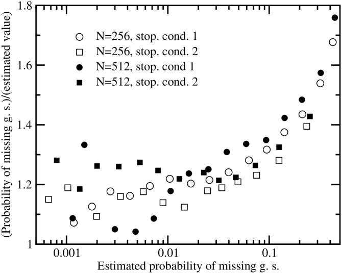
Figure 1: Ratio of the true and the estimated frequency of missing the ground state with different stopping conditions for samples of $N=256$ and $N=512$ SK systems. See text for details.

We calculated ground states of large samples between sizes of $N=64$ and $N=2048$ spins. Parameters of stopping condiditions, sample sizes, and the estimated probabilities of missing the ground state for instances with the Gaussian interaction are shown in Table 1. For $N=128$, $N=256$ and $N=512$ we made another complete series of calculations, which were longer, and even more reliable than the first one. We chose $n_{smax}$ very large, increased $n_{smin}$ to 2000 for $N=128$ and $N=256$, and to 4000 for $N=512$, and we applied $M_{req}=80$, $M_{req}=50$ and $M_{req}=50$ for $N=128$, $N=256$ and $512$, respectively. For N=$128$ all 500000 results agreed, while for $N=256$ and for $N=512$ the longer series improved 6 (0.003%) and 4 (0.01%) cases, respectively, which is a marginal fraction. For $N=256$ and $N=512$ we derived what energies we would have ended up if we had applied stopping conditions of type 1 and type 2 with a variety of $n_{s}$ (between 1 and 194 for N=$256$ and between 4 and 880 for $N=512$) and $M_{req}$ (between 2 and 29) values, respectively. As we have every reason to believe that we know the true ground states of these systems, except for may be a negligible fraction, we know in each case how often the states accepted were not the ground states. Then following the recipe we proposed above, we estimated the error rates by finding out how frequently repeated runs would have failed to find the same or a better energy with the same stopping conditions. Fig. 1 shows the factors we have to multiply the estimated rate of missing the ground state to get the true error rate in case of the different stopping conditions considered. The figure shows that we do not underestimate very much the true error rates. For rates less than about 10%, this factor is about $1.2$. It would probably steadily decrease with the error rate, but our samples are not large enough to tell how fast. It decreases much slower than it would if all samples of the same size were equally hard (in that case the difference between the true and estimated rate would be about the square of the rate, so for an error rate of $\delta$ the factor shown on the figure would be about $1+\delta$). Therefore, the error rates shown in Table 1 must be very good order of magitude estimates. Even if the true rates were larger by a factor of 2 or 3 instead of the about 20% we believe, it would have a very small effect on the average ground state energies and on the width of the ground state energy distribution. Nevertheless, the argument presented here can not be taken as a strict proof of reliability of the method. To find out how much we underestimate error rate, we supposed that the long enough calculations were really very reliable, i. e.  when we see the error rate going to zero, it really does so. However, if the true ground states of a finite proportion of the instances were so difficult for the algorithm to find, that they would not even start appearing in any calculation of a reasonable length, the assumption would not hold. We have no reason to believe that the present spin glass problem were so pathological, therefore we think that the circumstancial evidence for the reliability of the algorithm is strong enough.

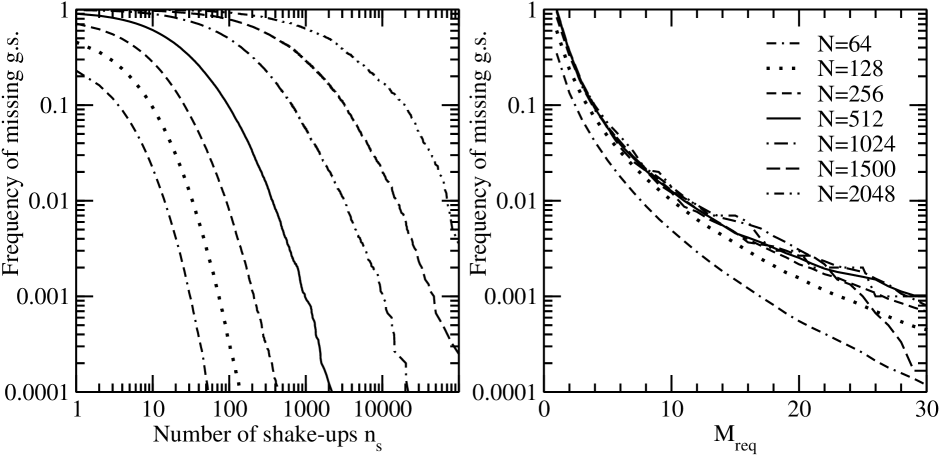
Figure 2: Frequency of not finding the ground state after a fixed number of shake-ups $n_{s}$ (stopping condition type 1), and after the current best state state has been found $M_{req}$ times (stopping condition type 2).

In Fig. 2 we show estimated error rates for different system sizes with type 1 stopping condition as the function of the number of shake-ups $n_{s}$ and with type 2 stopping condition as the function of the number of times $M_{req}$ we require to find the lowest state before accepting it as the ground state. We can see that the number of shake-ups we need to reach the same reliability grows pretty fast with $N$. Therefore, making reliable large scale calculations for systems much larger that $N=2000$ is fairly hopeless with the present algorithm. It is interesting to note that with the type 2 stopping condition the reliability of the results with a given $M_{req}$ does not seem to depend on the system size $N$ if $N$ is large enough. If this is not an accident, it may be a further indication that the results are reliable even for the largest system sizes.

Now we discuss shortly some of our results on the behaviour of the average energy per spin $\langle E(N)/N\rangle$, and the standard deviation of its distribution $\sigma_{E/N}$. A more detailed analysis and a discussion of the distribution functions will be published in a separate paper. The energy per spin is expected to converge to the asymptotic value with an exponent $\omega$. This exponent for scaling corrections is not known analytically. Near $T_{c}$ a value of $2/3$ has been derived [21], and numerical studies on smaller systems have been compatible with this value for the behaviour of the ground state energy as well [22, 23, 24, 15]. For the asymptotic value of $\langle E/N\rangle$ exact result is available [25, 26]. We substracted this value of -0.76321 from our results for $\langle E/N\rangle$, and multiplied it with $N^{2/3}$. The result as a function of $N$ is shown in Fig. 3, for both the Gaussian and the $\pm J$ case. We would expect to see horizontal lines if $\omega=2/3$. The energy clearly converges faster to the asymptotic value than expected, which means that either $\omega$ is larger than $2/3$, or even with these system sizes we are still not in the asymptotic region, and subleading corrections are important. Some deviation has been noted in Ref. [24] as well.

The width of the energy per spin distribution converges to zero as $N^{-\rho}$. The exponent $\rho$ is also unknown analytically. Ref. [27] predicted $\rho=5/6$. Since then, numerical results [28, 22, 24, 15] and qualitative arguments [22, 29] indicated the smaller value of $\rho=3/4$. We show our results multiplied by $N^{3/4}$ in Fig. 3. Convergence is again faster than expected if $\rho=3/4$, which again means either a larger $\rho$ value, or important subleading corrections. Boettcher, whose results also started to show deviations from the expected behaviour [15], argued in favour of the latter possibility. He showed that $\sigma_{E/N}N^{3/4}$ as a function of $N^{-1/4}$ can well be approximated with a parabola, which indicates corrections in powers of $N^{-1/4}$. This is actually true for our results with larger systems and larger samples as well, therefore $\rho=3/4$ with further corrections is a possibility. However, $\sigma_{E/N}N^{5/6}$ as a function of $N^{-1/6}$ may also be well approximated with a parabola, which means that $\rho=5/6$ [27] is also possible by the same argument. We note that the parabola indicates not one, but two further non-negligible correction terms. Actually, if $\rho$ is a simple rational number, for systems larger than a few hundred spins, our results are most compatible with $\rho=4/5$. For those larger $N$ values $\sigma_{E/N}N^{4/5}$ is horizontal with a very good approximation, and no further corrections are needed.

We note that the faster than expected convergence of both the energy and the width can not be explained by supposing that our ground states are less reliable than we think. If we do shorter runs and miss more ground states we get higher values for both the average and the standard deviation. For the average this is trivial, and for the standard deviation it is not surprising either that extra randomness will tend to increase the spread. As we surely make errors more often for larger systems than for smaller ones, those errors would make the convergence of the quantities slower.

5 Conclusion

We have demonstrated in the present paper that hysteretic optimization is very well suited for finding ground states of Sherrington–Kirkpatrick spin glasses. The algorithm makes it possible to handle large samples of systems up to sizes of about 2000 with affordable computational effort. The method we applied to estimate the proportion of true ground states missed may be useful also for other algorithms based on repeating many times the same procedure containing stochastic elements. Our results show that the average ground state energy and the width of the ground state energy distribution converges faster than expected, which may either indicate larger exponents, or important further correction terms.

Table 1: Details of hysteretic optimization runs for the SK model with Gaussian interactions. System size $N$, sample size, the minimum and the maximum number of shake-ups $n_{smin}$ and $n_{smax}$, respectively, the required number of finding the lowest state before accepted as ground state $M_{req}$, the average CPU time (2.8 GHz P4) per instance $\langle t\rangle$ (the actual time varies in a wide interval) and the estimated probability of missing the ground state (see text, the actual value is probably higher by about a factor of 1.2).

$N$	sample	$n_{smin}$	$n_{smax}$	$M_{req}$	$\langle t\rangle$	error
64	1000000	200	10000	60	0.06s	0
128	500000	200	10000	60	0.41s	0.001%
256	200000	400	10000	40	2.66s	0.004%
512	40000	1500	15000	30	38.6s	0.013%
1024	15000	1500	15000	20	8.17m	0.23%
1500	6000	3000	30000	15	45.7m	0.58%
2048	1000	10000	90000	15	417.m	1.10%

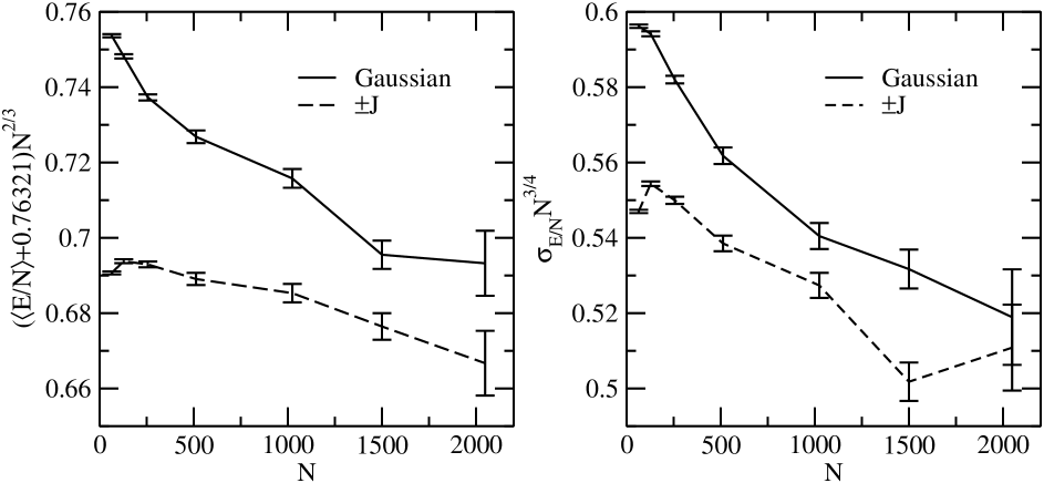
Figure 3: The dependence of the average energy per spin and the width of its distribution on the size of the system. From the energy the known asymptotic value is subsctracted, and the functions are multiplied by factors such that they should behave as constants.

References

- [1] G. Zaránd, F. Pázmándi, K.F. Pál, and G.T. Zimányi, Phys. Rev. Lett. 89, 150201 (2002).
- [2] K.F. Pál, in New Optimization Algorithms in Physics, eds. A.K. Hartmann and H. Rieger, (Wiley-VCH, Weinheim, 2004), 205.
- [3] K.F. Pál, Physica A, 360, 525 (2006).
- [4] K.F. Pál, Physica A, 329, 287 (2003).
- [5] S. Kirkpatrick, C.D. Gelatt, Jr. and M.P. Vecchi, Nature 220, 671 (1983).
- [6] K.F. Pál, Physica A 223, 283 (1996).
- [7] K.F. Pál, Physica A 233, 60 (1996).
- [8] A.K. Hartmann, Europhys. Lett. 40, 429 (1997).
- [9] A.K. Hartmann, Phys. Rev. E 59, 84 (1999).
- [10] J. Houdayer, O.C. Martin, Phys. Rev. Lett. 83, 1030 (1999).
- [11] J. Houdayer, O. C. Martin, Phys. Rev. E 64, 056704 (2001).
- [12] S. Boettcher, A.G. Percus, Phys. Rev. Lett. 86, 5211 (2001).
- [13] A.A. Middleton, Phys. Rev. E 69, 055701(R) (2004).
- [14] m. J. Alava,V. Basso,F. Colaiori, L. Dante, G. Durin, A. Magni, S. Zapperi, Phys. Rev. B 71, 064423 (2005).
- [15] S. Boettcher, Eur. Phys. J. B 44, 317 (2005).
- [16] S. Kobe, cond-mat/0311657.
- [17] H. R. Lourenco, O. C. Martin, T. Stutzle, in Handbook of Metaheuristics, eds. F. Glover and G. Kochenberger, (Kluwer Academic Publishers, Norwell, 2002), 321.
- [18] S. Boettcher, A.G. Percus, Phys. Rev. E 69, 066703 (2004).
- [19] M. Palassini, A. P. Young, Phys. Rev. Lett. 83, 5126 (1999).
- [20] O. C. Martin, in New Optimization Algorithms in Physics, eds. A.K. Hartmann and H. Rieger, (Wiley-VCH, Weinheim, 2004), 23.
- [21] G. Parisi, F. Ritort, F. Slanina, J. Phys. A bf 26, 3775 (1993).
- [22] J.-P. Bouchaud, F. Krzakala, O. C. Martin, Phys. Rev. B 68, 224404 (2003).
- [23] M. Palassini, PhD thesis, 2000.
- [24] M. Palassini, cond-mat/0307713.
- [25] G. Parisi, Phys. Rev. Lett. bf 43, 1754 (1979); bf 50, 1946 (1983).
- [26] A. Crisanti, T. Rizzo, Phys. Rev. E bf 65, 046137 (2002).
- [27] I. Kondor, J. Phys. A bf 16, L127 (1983).
- [28] S. Cabasino, E. Marinari, P. Paolucci, G. Parisi, J. Phys. A bf 21, 4201 (1988).
- [29] T. Aspelmeier, M. A. Moore, A. P. Young, Phys. Rev. Lett. bf 90, 127202 (2003).