Abstract

Two families of cuprates exhibiting high-$T_{c}$ superconductivity, YBa₂Cu₃O_6+x (YBCO) and La_2xSr_xCuO_4+δ (LSCO), have been extensively studied by anelastic spectroscopy, by measuring the complex dynamic Young’s modulus $E\left(\omega,T\right)=E^{\prime}+iE^{\prime\prime}$ of ceramic samples at frequencies of 0.5-20 kHz between 1 and 900 K. Results are also presented on oxygen vacancies in the ruthenocuprate RuSr₂GdCu₂O_8-δ. The elastic energy loss curves as a function of temperature, $Q^{-1}\left(\omega,T\right)=$ $E^{\prime\prime}/E^{\prime}$, contain peaks at the temperatures $T_{m}$ such that $\omega\tau(T_{m})~{}\simeq$ 1, where $\omega/2\pi$ is the measuring frequency and $\tau$ is the relaxation time of any microscopic process coupled to strain, like hopping of O atoms, tilting of O octahedra or fluctuations of the hole stripes. By measuring such anelastic spectra at different frequencies, it is therefore possible to selectively probe the dynamics of the various relaxation processes, precisely determining their characteristic times $\tau\left(T\right)$. The reliability of the anelastic experiments and of the assignments to various microscopic mechanisms is also discussed.

The richest anelastic spectra are those of LSCO, and have been studied in the whole range of Sr doping ($0<x<0.2$) and at few Ba doping levels. As in the parent perovskite compounds, LSCO is made of O octahedra unstable against tilting, which give rise to low symmetry phases. The layered coordination of such octahedra and the possibility of achieving a low density of pinning defects (interstitial O atoms), makes it possible to observe solitonic tilt waves and fast local motion of the octahedra among the several minima of the local tilt potential far below the structural transition temperature. The fast local motion is driven by tunneling of the O atoms and is enormously enhanced and accelerated by even small doping, demonstrating direct coupling between the tilt modes of the octahedra and the hole excitations.

In addition, it has been possible to probe the dynamics of the stripes into which the holes segregate, at liquid He temperature, when they act as walls between domains of antiferromagnetically correlated spins (cluster spin glass), and also at higher temperature, when they can overcome by thermal activation the pinning barriers provided by Sr²⁺ dopants. A picture is proposed in which the high temperature motion of the stripes involves the formation of kink pairs, while at lower temperature only the motion of the existing kinks can occur.

In YBCO the anelastic spectra are dominated by the motion of the O atoms in the CuO_x planes, which are responsible for the doping of the charge carriers (holes) into the superconducting CuO₂ planes. The doping level, and therefore the superconducting properties, are determined not only by the content $x$ of highly mobile non-stoichiometric O, but also by its ordering. The various processes involved in ordering and diffusion of O have different characteristic times $\tau$, and therefore produce distinct peaks in the anelastic spectra at the temperatures for which $\omega\tau(T_{m})=$ 1; they have been studied in the whole stoichiometry ($0<x<1$) and temperature (50 K $<T<800$ K) ranges. It is shown that there are three types of O jumps with different rates, depending whether they involve: i) ordered Cu-O chains in the orthorhombic O-I phase ($x$ $\sim$ 1); ii) sparser chains fragments in the O-II and tetragonal phases; iii) isolated O atoms. The first two types of jumps occur over a barrier of $\sim$1.0 eV, whereas the latter has a barrier of only 0.11 eV. It is discussed how such widely different barriers for O hopping are possible and how the extraordinarily high mobility of isolated O atoms is compatible with the slow times for O ordering. In addition to the diffusive jumps, hopping of O between off-center positions within the Cu-O chains is proposed to occur. Finally, an anelastic process has been observed, whose intensity increases steeply in the overdoped state, $x>0.9$, where all the other physical properties remain practically constant. Such a process is attributed to the reorientation of small bipolarons on orbitals that do not contribute to the electrical conduction, and can be useful for characterizing materials with non-optimal O content, like thin films.

RuSr₂GdCu₂O_8-δ is isostructural with YBCO, except for RuO_2-δ planes with $\delta$ below few percents instead of the widely nonstoichiometric CuO_x planes. In this case, the situation of O mobility and ordering is simpler than in YBCO, and it is shown that it can be quantitatively explained in terms of hopping of O vacancies whose elastic quadrupoles are weakly interacting and start becoming parallel to each other below $T_{\mathrm{C}}\sim 470$ K.

Bibliography

List of acronyms and symbols

Acknlowledgments

Chapter 1 Introduction

The cuprates exhibiting high-$T_{\text{c}}$ superconductivity (HTS) have been receiving enormous attention in the scientific literature, due to the great number of interesting physical effects they exhibit and to their technological applications such as Superconducting Quantum Interference Devices (SQUID) for highly sensitive measurements of magnetic fields, filters for the transmissions with mobile phones, or electric power applications [1]. Among the most studied and not yet completely understood issues are those connected with nonstoichiometric oxygen, its ordering and role in doping, and those connected with spin and charge inhomogeneities on the scale of nanometers, generally called stripes (see Ref. [2] for a recent review).

In HTS cuprates, superconductivity sets in mainly in CuO₂ planes doped with holes (or electrons in the case of Nd_2-xCe_xCuO_4+δ), and doping is due to the charge unbalance from aliovalent substitutional cations (e.g. Sr²⁺ in La_2-xSr_xCuO₄) and from nonstoichiometric oxygen (generally excess O^2-). The oxygen stoichiometry may be varied over relatively wide ranges, but the amount of charge doping depends also on the ordering of nonstoichiometric O atoms, which are the most mobile atomic species. For this reason, the detailed knowledge of the diffusion and ordering mechanisms of oxygen in the cuprates are of great interest, especially in materials of the YBa₂Cu₃O_6+x (YBCO) family where doping is totally due to oxygen. A host of studies have been carried out on the oxygen mobility and ordering, especially with diffraction and permeation from gas phase methods, revealing complex phase diagrams and non trivial effects. Anelastic spectroscopy is one of the most powerful methods to study these complex phenomena, thanks to its ability of selectively measuring different types of hopping rates, from isolated or differently aggregated O atoms, which produce different elastic energy loss peaks in the temperature scale.

The topic of the intrinsic charge and spin inhomogeneities in HTS cuprates is also of great interest; in fact, not only the observation that the conducting holes may segregate into fluctuating stripes is difficult from the experimental point of view and counterintuitive, but it is also debated whether it is a phenomenon competing against superconductivity [3] or instead is at the basis of HTS [4, 5, 6]. Rather unexpectedly, the anelastic measurements on cuprates of the LSCO family reveal also features attributable to the slow collective dynamics of charge stripes and antiferromagnetic domains in the CuO₂ planes, and, to my knowledge, they are the only experiments where some of these dynamic processes are observable at acoustic frequencies. In fact, ac magnetic susceptibility, and dielectric, NMR, $\mu$SR spectroscopies are dominated by the single charge or spin fluctuations, while anelastic spectroscopy is insensitive to them and may probe the collective charge and spin motions through their weak coupling to strain.

Two families of HTS cuprates, YBa₂Cu₃O_6+x (YBCO) and La_2-xSr_xCuO₄ (LSCO), have been extensively studied by anelastic spectroscopy, by measuring the complex dynamic Young’s modulus of ceramic samples at frequencies of 0.5-20 kHz between 1 and 900 K. In addition, some results are presented on the ruthenocuprate compund RuSr₂GdCu₂O₈ (Ru-1212). All the samples have been obtained from a collaboration with the Department of Chemistry and Industrial Chemistry of the University of Genova, Italy (M. Ferretti), while several anelastic experiments have been done in collaboration with the Physics Department of the University of Rome ”La Sapienza” (G. Cannelli, R. Cantelli, A. Paolone, F. Trequattrini).

Several phenomena have been found and studied, among which diffusive hopping, ordering and off-center dynamics of O atoms, collective and local tilt dynamics of the octahedra in LSCO, and charge stripe fluctuations and depinning. Unless otherwise specified, all the results presented here were the first studies of such phenomena by anelastic spectroscopy.

The Thesis is organized as follows. First is an introduction to anelasticity, limited to the concepts that are necessary for interpreting the phenomena discussed later, and emphasizing those concepts that are treated little in books on anelasticity; in particular, relaxation between energetically inequivalent states, interaction between elastic dipoles in the mean field approximation, and the relationship between anelastic and other spectroscopies. A brief description follows of the method of measurement and of the samples treatments. A chapter is devoted to LSCO, with a short description of its structural and magnetic phase diagram, with the unstable tilt modes of the oxygen octahedra, and of the charge and spin stripes. The anelastic measurements are presented starting with the phase transformations, then interstitial O, followed by the newly found relaxational dynamics of the unstable tilts of the octahedra, and finally the observations of the thermally activated depinning dynamics of the hole stripes and their motion in the cluster spin glass phase, identifiable with the motion of pinned domain walls between antiferromagnetic domains. The following chapter is devoted to YBCO, starting with a presentation of its complex structural phase diagram due to various types of ordering of O in the CuO_x planes, and of the main results in literature on the mobility of this oxygen species. Section 5.4 is devoted to the diffusive jumps of oxygen and starts with an overview of the anelastic spectra at different stoichiometries, followed by a discussion of what kind of effects one might expect from the interaction among oxygen atoms, at least in the simple Bragg-Williams approximation. Then, the three distinct elastic energy loss peaks due to the oxygen diffusive jumps are discussed, with emphasis on the extremely fast hopping rate of the isolated O atoms in the semiconducting state, and on the role of the charge transfer between Cu-O chains and CuO₂ planes in determining various types of O jumps; also the ordering dynamics of oxygen is discussed. The chapter on YBCO terminates with a relaxation process identified with the hopping of O between off-center position in the Cu-O chains, which diffraction studies suggest to be slightly zig-zag instead of straight, and with a peak which develops for $x>0.85$, a doping range where all the physical properties are practically constant, and attributed to reorientation of pairs of holes (bipolarons) in the apical O atoms.

The anelastic spectra of LSCO and YBCO reflect the great complexity of the structural, magnetic and charge phenomena occurring in these cuprates, and their interpretation is not always straightforward; therefore, at the end of the chapters devoted to LSCO and YBCO, a summary of the main results is provided, together with brief explanations of how the various anelastic effects have been assigned to specific mechanisms.

Finally, a chapter is devoted to the diffusive hopping of oxygen in the ruthenocuprate RuSr₂GdCu₂O_8-δ, where it is more appropriate to talk of oxygen vacancies, since in the RuO_2-δ planes the oxygen stoichiometry is rather stable and close to the maximum. In this case, therefore, there is no complex phase diagram for the oxygen ordering, and the hopping dynamics may be described in terms of interaction among the elastic dipoles in the mean-field approximation.

Chapter 2 Anelasticity

The anelastic spectroscopy consists in the measurement of the complex dynamic compliance, or its reciprocal, the elastic stiffness, generally as a function of temperature at fixed frequencies. It is the mechanical analogue of the dielectric spectroscopy or ac magnetic susceptibility. Comprehensive treatments of the theory of anelasticity and of the application of the anelastic spectroscopy to the study of solids can be found in the seminal book of C. Zener [7], in the classic book by Nowick and Berry [8] and in the most recent book edited by Schaller, Fantozzi and Gremaud [9]. The use of tensors for describing the elastic properties of solids can be found in books like Ref. [10, 11, 12]. In the present chapter I will only mention what is strictly necessary for defining the notation and for the comprehension of the results discussed in the Thesis, with emphasis on the issues that are not treated in the above texts.

2.0.1 Elastic dipole and thermodynamics of the relaxation

For a perfectly elastic solid, Hooke’s law can be written (in matrix instead of tensor notation) as

$$\varepsilon_{i}=s_{ij}\sigma_{j}$$ (2.1)

where $\varepsilon_{i}$ and $\sigma_{i}$ are components of the strain and stress tensors and $s_{ij}$ the elastic compliance matrix, and summation over repeated indices is understood, or equivalently

$$\sigma_{i}=c_{ij}\varepsilon_{j}\,$$ (2.2)

where $c_{ij}$ is the stiffness matrix. In matrix notation, index $i=1,2,3$ denote uniaxial strains along $x,y$ and $z$ respectively, while $i=4,5,6$ denote shears of type $yz,xz$ and $xy$ (see Fig. 2-1a,b; note that a shear strain is equivalent to two perpendicular uniaxial strains at 45^o with different sign and equal magnitude, as shown by the gray arrows). Anelasticity results from the response to the application of a stress from defects or excitations that can change their state and also their contribution to the overall strain, with a characteristic relaxation time $\tau$; then, the elastic response according to the above equations is accompanied by a retarded anelastic response.

For simplicity, I will refer to a molar concentration $c$ of point defects uniformly distributed over the solid, and having at least two possible states; e.g. interstitial atoms that visit sites of type 1 and 2, according whether the first neighboring lattice atoms along the $x$ or $y$ directions (Fig. 2-1c).

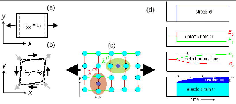
Figure 2-1: (a) Uniaxial and (b) shear strains. (c) Interstitial atoms and corresponding elastic dipoles under the application of a uniaxial $\sigma_{1}$ stress and (d) effect of $\sigma_{1}$ on the defects and strain.

One then defines the concentrations $c_{1}$ and $c_{2}$ of defects in states 1 and 2, with $c_{1}+c_{2}=c$ and their specific contributions to strain

$$\lambda_{ij}^{(\alpha)}=\frac{\partial\varepsilon_{ij}}{\partial c_{\alpha}}$$ (2.3)

where $\lambda_{ij}^{(\alpha)}$ is the elastic dipole of the defects of type $\alpha$. The definition ”elastic dipole” derives from the analogy with the electric or magnetic dipoles of polar or magnetic defects [8], but, being a centrosymmetric strain tensor of the 2nd rank and not a vector, it is actually a quadrupole [11] representable as an ellipsoid with the principal axes defined by the tensor eigenvalues. This is shown in Fig. 2-1c for interstitial atoms causing greater lattice expansion in the direction of the nearest neighbor atoms. From Eq. (2.3) it follows that the anelastic strain is

$$\varepsilon_{ij}^{\text{an}}=\sum_{\alpha}c_{\alpha}\lambda_{ij}^{(\alpha)}\;\,.$$ (2.4)

From now on I will drop the tensor indices unless necessary, and assume that a pure type of stress is applied, e.g. uniaxial, and the corresponding components of strain and compliance are probed.

It is easy to show with a thermodynamic argument that the elastic dipole is also minus the rate of change of the elastic energy of a defect on application of stress. In fact, the differential of the Gibbs free energy $g$ per unit volume (all the extensive variables are expressed per unit volume) is:

$$dg=-\varepsilon d\sigma-sdT+\frac{1}{v_{0}}\sum_{\alpha}E_{\alpha}dc_{\alpha}$$ (2.5)

where $v_{0}$ is the molecular volume and $s$ here is the entropy per unit volume; differentiating twice one obtains that

$$\lambda^{\left(\alpha\right)}=\frac{\partial\varepsilon}{\partial c_{\alpha}}=-\frac{\partial^{2}g}{\partial c_{\alpha}\partial\sigma}=-\frac{1}{v_{0}}\frac{\partial E_{\alpha}}{\partial\sigma}.$$ (2.6)

and therefore the application of a stress $\sigma$ changes the defect elastic energy as

$$E_{\alpha}\left(\sigma\right)=E_{\alpha}\left(0\right)-v_{0}\lambda^{\alpha}\sigma\,.$$ (2.7)

The defects occupy the possible states (or energetic levels) according to some distribution function and, for the sake of simplicity, let us considered diluted defects whose populations obey the Boltzmann distribution function; then

$$c_{\alpha}=c\frac{e^{-E_{\alpha}/k_{\text{B}}T}}{Z}\,,\quad Z=\sum_{\alpha}e^{-E_{\alpha}/k_{\text{B}}T}.$$ (2.8)

The application of a stress $\sigma$ (see Fig. 2-1c and d) changes the energies $E_{\alpha}\left(\sigma\right)$ of

$$\delta E_{\alpha}=\sigma\frac{\partial E_{a}}{\partial\sigma}=-v_{0}\lambda^{\left(\alpha\right)}\sigma$$ (2.9)

and the new thermal equilibrium requires a repopulation of the states (with a relaxation time $\tau$) such that

$$\delta c_{\alpha}=\sum_{\beta}\frac{\partial c_{\alpha}}{\partial E_{\beta}}\frac{\partial E_{\beta}}{\partial\sigma}\sigma=-\sum_{\beta}\frac{\partial c_{\alpha}}{\partial E_{\beta}}\,v_{0}\lambda^{\left(\beta\right)}\sigma\,,$$ (2.10)

which results in the anelastic strain

$$\varepsilon^{\text{an}}=\sum_{\alpha}\lambda^{\left(\alpha\right)}\,\delta c_{\alpha}=-v_{0}\sum_{\alpha}\sum_{\beta}\frac{\partial c_{\alpha}}{\partial E_{\beta}}\lambda^{\left(\alpha\right)}\lambda^{\left(\beta\right)}\,\sigma$$ (2.11)

It can be shown [13] that (the case of only two states is trivial)

$$\varepsilon^{\text{an}}=v_{0}\sigma\sum_{\text{pairs }\alpha<\beta}c\frac{n_{\alpha}n_{\beta}}{k_{\text{B}}T}\left(\lambda^{\left(a\right)}-\lambda^{\left(\beta\right)}\right)^{2}$$ (2.12)

where $n_{\alpha}=c_{\alpha}/c$, which can also be extended to non-Boltzmann statistics [13]. The relaxation strength is defined as

$$\Delta=\frac{\varepsilon^{\text{an}}}{\varepsilon^{\text{el}}}=\frac{v_{0}}{s}\sum_{\text{pairs }\alpha<\beta}c\frac{n_{\alpha}n_{\beta}}{k_{\text{B}}T}\left(\lambda^{\left(a\right)}-\lambda^{\left(\beta\right)}\right)^{2}=\sum_{\text{pairs }\alpha<\beta}\Delta_{a\beta}$$ (2.13)

and this equation tells us that i) the anelastic response is the sum of the partial contributions $\Delta_{\alpha\beta}$ from the repopulation of all the pairs of defect states; ii) $\Delta_{\alpha\beta}$ is proportional to the square of the anisotropy of the elastic dipole $\left(\lambda^{\left(\alpha\right)}-\lambda^{\left(\beta\right)}\right)^{2}$ and therefore elastically equivalent states ($\lambda^{\left(\alpha\right)}=\lambda^{\left(\beta\right)}$) are not repopulated with respect to each other and do not cause relaxation; iii) $\Delta_{\alpha\beta}$ is proportional to the defect concentration but also to the depopulation factor $n_{\alpha}n_{\beta}$, meaning that if the two states $\alpha$ and $\beta$ are energetically inequivalent also in the absence of stress, then one of the two is less populated and this limits the stress-induced repopulation and the relaxation intensity. Note that in case of high density of defects [13], the term $n_{\alpha}n_{\beta}$ becomes of the type $n_{\alpha}\left(1-n_{\alpha}\right)n_{\beta}\left(1-n_{\beta}\right)$ since e.g. the jump of a defect from a site $\alpha$ to a site $\beta$ is proportional to $n_{\alpha}$ but also requires that site $\beta$ is empty, hence the term $\left(1-n_{\beta}\right)$, and analogously for the $\beta\rightarrow\alpha$ transitions. Such expressions are also symmetric in $n_{\alpha}$ and $1-n_{\alpha}$, meaning that, e.g. when dealing with the jumps of the O atoms in the CuO_2c or RuO_2c planes of YBCO or Ru-1212 ($0<c<1$) for $c\rightarrow 0$ the O atoms are the defects, but for $c\rightarrow 1$ the O vacancies can rather be considered as the defects. Finally, the $1/k_{\text{B}}T$ term comes from $\frac{\partial n_{\alpha}}{\partial E_{\beta}}\propto\left(k_{\text{B}}T\right)^{-1}$, which is a consequence of the fact that with increasing temperature all the defect states tend to become equiprobable.

For the case of relaxation between only two states with

$$\Delta\lambda=\lambda_{2}-\lambda_{1}\,,\quad\Delta E=E_{2}-E_{1}$$ (2.14)

one obtains

$$\Delta\left(T\right)=\frac{v_{0}c\left(\Delta\lambda\right)^{2}}{4s\,k_{\text{B}}T\,\cosh^{2}\left(\Delta E/2k_{\text{B}}T\right)}$$ (2.15)

which further reduces to the well known expression

$$\Delta\left(T\right)=\frac{v_{0}c\left(\Delta\lambda\right)^{2}}{4s\,k_{\text{B}}T\,}$$ (2.16)

for equivalent states with $\Delta E=0$. The term $\cosh^{-2}\left(\Delta E/2kT\right)$, coming from the depopulation factor $n_{1}n_{2}$ in Eq. (2.13) is generally overlooked, but becomes very important in all situations in which $\Delta E\sim k_{\text{B}}T$, since it produces a maximum in $\Delta\left(T\right)$ at $T=0.65\Delta E/k_{\text{B}}$ and then falls off as $\exp\left(-\Delta E/k_{\text{B}}T\right)$ for $T\rightarrow 0$. For example, when dealing with jumps of the O atoms in the CuO_x planes of YBCO, oxygen can pass from the isolated to the aggregated state and vice versa, which might well differ in energy by several tenths of electronvolt, which means thousands of kelvin in the temperature scale (I will often measure the energy in Kelvin, by considering $E/k_{\text{B}}$ instead of $E;$ the conversion is 1 eV = 11600 K); the $\cosh^{-2}\left(\Delta E/2kT\right)$ term would cause a reduction of $\Delta\left(T=500~{}\text{K}\right)$ by a factor 0.04 for $\Delta E\sim 0.2$ eV and a factor $0.004$ for $\Delta E\sim 0.3$ eV, making certain types of jumps completely unobservable in the anelastic relaxation.

The depopulation factor becomes important at low enough temperature even for relaxation between states that ideally are energetically equivalent; in fact, unless dealing with extremely low concentrations of impurities in crystals of high perfection, there will always be long range elastic interactions among defects that cause random shifts $\Delta E$ to the defect energies. Such shifts have been estimated for the case of O-H pairs in Nb to be of the order of 100 K for impurity concentrations of $\sim 1$ at% [14]. This means that, especially for disordered solids like the HTS, relaxation processes below 100 K are very likely affected by the depopulation factor, whose effect is of changing the temperature dependence of the relaxation intensity from $T^{-1}$ to a nearly constant or increasing function of $T$. In such cases, I will include the depopulation factor in the analysis.

2.0.2 Relaxation kinetics

There is no general treatment for the relaxation kinetics and I will limit to the relaxation between two states from the start. In this case the rate equations for the defect populations are

$$\left\{\begin{array}[c]{c}\dot{n}_{1}=-\nu_{21}n_{1}+\nu_{12}n_{2}\\ \dot{n}_{2}=+\nu_{21}n_{1}-\nu_{12}n_{2}\end{array}\right.\,$$ (2.17)

with $\nu_{ij}$ the rate for passing from $j$ to $i$; thanks to the condition $n_{1}+n_{2}=1$ there is actually one independent $n_{i}$. Setting $\dot{n}_{i}=0$ the equilibrium populations are found as

$$\overline{n}_{i}=\frac{\nu_{ij}}{\nu_{12}+\nu_{21}}\,,$$ (2.18)

which agree with the thermodynamic result if $\nu_{12}$ e $\nu_{21}$ satisfy the detailed balance principle

$$\frac{\overline{n}_{1}}{\overline{n}_{2}}=\frac{\nu_{12}}{\nu_{21}}=e^{\Delta E/k_{\text{B}}T}\text{\thinspace.}$$ (2.19)

Incidentally, Eq. (2.19) requires that, for hopping over a saddle point $E_{\text{s}}$ according to the Arrhenius law,

$$\nu_{ij}=\frac{1}{2}\tau_{0}^{-1}\exp\left(\frac{E_{\text{s}}-E_{j}}{k_{\text{B}}T}\right)$$ (2.20)

with the same $\tau_{0}$ for both states. Defining

$$\Delta n=n_{2}-n_{1}\,,$$ (2.21)

the previous equations can be put in the form

$$\Delta\dot{n} =-\frac{\Delta n-\Delta\overline{n}}{\tau}$$ (2.22a)

$$\tau^{-1} =\left(\nu_{12}+\nu_{21}\right)=\tau_{0}^{-1}\exp\left(-E/k_{\text{B}}T\right)\cosh\left(\Delta E/2k_{\text{B}}T\right)$$ (2.22b)

which says that the rate for $$\Delta n \Delta\overline{n} \Delta\overline{n} \tau^{-1} E=E_{\text{s}}-\frac{1}{2}\left(E_{1}+E_{2}\right) \cosh\left(\Delta E/2k_{\text{B}}T\right)$$ reaching the equilibrium value is proportional to its deviation from through the relaxation rate ; the latter has been written in terms of the mean activation energy and therefore contains a factor that should be taken into account when dealing with asymmetric states.

On application of a time dependent stress $\sigma\left(t\right)$, there will be an instantaneous elastic response

$$\varepsilon^{\text{el}}\left(t\right)=s_{\text{U}}\sigma\left(t\right)$$ (2.23)

where subscript ”U” stands for unrelaxed, and in addition an anelastic strain $\varepsilon^{\text{an}}=$ $c\left(n_{1}\lambda_{1}+n_{2}\lambda_{2}\right)=$ $c\left[\frac{\lambda_{1}+\lambda_{2}}{2}+\frac{1}{2}\Delta\lambda\Delta n\right]$ where the first term is constant and the time dependent anelastic response is

$$\varepsilon^{\text{an}}\left(t\right)=\frac{c}{2}\Delta\lambda\Delta n\left(t\right)$$ (2.24)

with $\Delta n$ determined by Eq. (2.22a).

2.0.3 Dynamic compliance

Let us calculate the time dependent anelastic response Eq. (2.24) on application of a periodic stress $\sigma=\sigma_{0}e^{i\omega t}$ that modulates $\Delta E$. It is convenient to refer $\Delta n$ to the equilibrium values in the absence of stress, defining:

$$\Delta n^{\prime}=\Delta n-\Delta\overline{n}\left(\sigma=0\right)$$ (2.25)

and for the instantaneous equilibrium $\Delta\overline{n}=-\tanh\left(\Delta E/2k_{\text{B}}T\right)$

$$\Delta\overline{n}^{\prime}=\Delta\overline{n}-\Delta\overline{n}\left(\sigma=0\right)=\frac{d\Delta\overline{n}}{d\Delta E}\frac{d\Delta E}{d\sigma}\sigma=\frac{v_{0}\Delta\lambda}{2k_{\text{B}}T\cosh^{2}\left(\Delta E/2k_{\text{B}}T\right)}\sigma$$ (2.26)

By substituting into Eq. (2.22a)

$$\Delta n^{\prime}=\frac{v_{0}\Delta\lambda\sigma}{2k_{\text{B}}T\cosh^{2}\left(\Delta E/2k_{\text{B}}T\right)}\frac{1}{1+i\omega\tau}$$ (2.27)

and using Eqs. (2.23,2.24) the dynamic compliance can be written as

$$s\left(\omega\right)=s^{\prime}-is^{\prime\prime}=\frac{\varepsilon^{\text{el}}+\varepsilon^{\text{an}}}{\sigma}=s_{\text{U}}\left[1+\frac{\Delta\left(T\right)}{1+i\omega\tau}\right]$$ (2.28)

where $\Delta\left(T\right)$ is the same as given by Eq. (2.15). The real and imaginary parts of $s\left(\omega\right)$ are therefore

$$s^{\prime}\left(\omega,T\right) =s_{\text{U}}\left[1+\frac{\Delta\left(T\right)}{1+\left(\omega\tau\right)^{2}}\right]$$ (2.29)

$$s^{\prime\prime}\left(\omega,T\right) =s_{\text{U}}\Delta\left(T\right)\frac{\omega\tau}{1+\left(\omega\tau\right)^{2}}$$

where the $s^{\prime\prime}$ presents the well known Debye peak of amplitude $\frac{1}{2}\Delta\left(T\right)$ at the condition for maximum relaxation

$$\omega\tau=1\,,$$ (2.30)

while $s^{\prime}$ a step of amplitude $\Delta\left(T\right)$. In the $\omega\tau\gg 1$ limit the defects are too slow to follow the periodic stress and corresponds to the elastic limit without defects ($s^{\prime}=s_{\text{U}}$, $s^{\prime\prime}=0$). In the $\omega\tau\ll 1$ limit the defect relaxation is so fast that instantaneously complies to the periodic stress, $s^{\prime\prime}=0$, and the compliance is totally relaxed, $s^{\prime}=s_{\text{U}}\left(1+\Delta\right)$.

It is possible to make an analogous derivation for the dynamic stiffness

$$c\left(\omega,T\right)=c^{\prime}+ic^{\prime\prime}\,,$$ (2.31)

finding

$$c^{\prime} =c_{\text{U}}\left(1-\frac{\Delta\left(T\right)}{1+\left(\omega\tau\right)^{2}}\right)$$ (2.32)

$$c^{\prime\prime} =c_{\text{U}}\Delta\left(T\right)\frac{\omega\tau}{1+\left(\omega\tau\right)^{2}}$$

2.1 Elastic energy loss and anelastic spectrum

The fact that the dynamic compliance $s\left(\omega,T\right)$ or stiffness $c\left(\omega,T\right)$ is complex means that, due to the retarded anelastic response, strain is out-of-phase with respect to stress by the loss angle

$$\tan\phi=\frac{s^{\prime\prime}}{s^{\prime}}=\frac{c^{\prime\prime}}{c^{\prime}}\,.$$ (2.33)

Generally, it is $\Delta\left(T\right)\ll 1$ so that

$$\tan\phi\simeq\frac{s^{\prime\prime}}{s_{\text{U}}}=\Delta\left(T\right)\frac{\omega\tau}{1+\left(\omega\tau\right)^{2}}\,.$$ (2.34)

The tangent of the loss angle can be measured from the dissipation of elastic energy or acoustic absorption; in fact, if $\sigma=\sigma_{0}\cos\left(\omega t\right)$ and $\varepsilon=\varepsilon_{0}\cos\left(\omega t-\phi\right)$, the elastic energy dissipated in one vibration cycle is

$$\Delta W=\int_{\omega t=0}^{\omega t=2\pi}\sigma d\varepsilon=\pi\varepsilon_{0}\sigma_{0}\sin\phi$$

while the maximum elastic energy stored is $W=\int_{\omega t=0}^{\omega t=\pi/2}\sigma d\varepsilon^{\prime}=$ $\frac{1}{2}\varepsilon_{0}\sigma_{0}\cos\phi$, where $\varepsilon^{\prime}=\varepsilon_{0}\cos\phi\cos\left(\omega t\right)$ is the strain component in phase with $\sigma$. One defines the elastic energy loss coefficient as

$$Q^{-1}=\frac{1}{2\pi}\frac{\Delta W}{W}=\tan\phi\,\text{,}$$ (2.35)

which coincides with the reciprocal of the mechanical $Q$ of the sample.

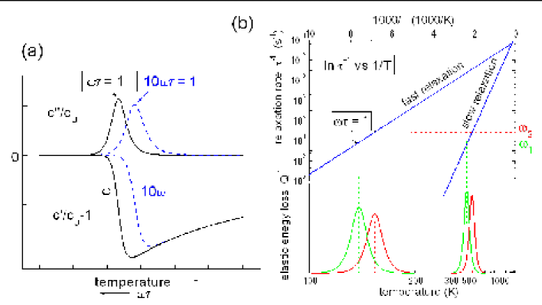
Figure 2-2: (a) Contribution of a Debye relaxation process to the imaginary and real parts of the dynamic stiffness at two measuring frequencies. (b) Anelastic spectrum with two processes having the relaxation rates plotted in the upper part; measured at the two frequencies $\omega_{1}$ and $\omega_{2}$.

Generally, the anelastic measurements are made sweeping temperature at nearly fixed frequency $\omega$, and the resulting spectrum contains absorption peaks in correspondence with the temperatures $T_{\text{max}}$ for which the condition of maximum relaxation $\omega\tau\left(T_{\text{max}}\right)=1$ is verified, while $c^{\prime}$ ($s^{\prime}$) contain negative (positive) steps. This is shown in Fig. 2-2, assuming that the relaxation rates follow the Arrhenius law, $\tau^{-1}=\tau_{0}^{-1}\exp\left(E/k_{\text{B}}T\right)$, between states with the same energy, so that $\Delta\left(T\right)\propto 1/T$. Figure 2-2b shows how slower processes are peaked at higher temperature, and how it is possible to estimate the energy barrier $E$ by measuring at different frequencies, exploiting the condition $\tau\left(T_{\text{max}}\right)=\omega^{-1}$ at the peak temperatures.

It is more convenient to analyze the $Q^{-1}\left(\omega,T\right)$ curves rather than the real parts $s^{\prime}\left(\omega,T\right)$ or $c^{\prime}\left(\omega,T\right)$, especially if $\Delta$ is very small, because the absorption peaks stand out of a usually small background (at least for $\omega<10$ MHz, when anharmonic effects and sound wave diffraction at the boundaries are small); instead, even for a perfectly elastic solid, the real part $s_{\text{U}}\$or $c_{\text{U}}$ has a temperature dependence due to anharmonic effects that should be subtracted in order to analyze the anelastic contribution. In addition, the elastic moduli are affected by the sample porosity, by microcracks, and internal stresses due to anisotropic thermal expansion building up during thermal cycling, which may result in anomalies and hystereses on varying temperature.

Figure 2-3 presents an example of anelastic spectrum measured on LSCO at three resonance frequencies during the same run; the stiffness which is measured is the Young’s modulus $E$. Note that the scale of the real part is almost 10 times larger than that of the absorption. Note also that the amplitudes of the steps in the real part are larger than $2\Delta$ deduced from the amplitudes $\Delta$ of the corresponding absorption peaks, as one expects from Eq. (2.29). This is due to the fact that the relaxation processes are broadened by distributions of relaxation times; the elementary peaks are shifted with respect to each other, so that the resulting peak resulting step in $E^{\prime}$ is the sum of the elementary steps.

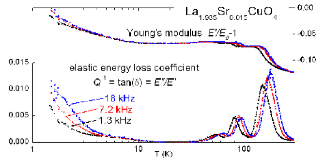
Figure 2-3: Example of anelastic spectrum (real and absorption parts) of LSCO measured at three vibration frequencies during the same run.

The pre-exponential factor $\tau_{0}^{-1}$ in the Arrhenius law is the relaxation rate extrapolated to infinite temperature, and its value deduced from experiments at low temperature should not be taken too seriously, since one should also take into account the temperature dependence of all the quantities that affect the jump rate, including the vibration entropies. Still, as a rule of thumb, $\tau_{0}\sim 10^{-13}$ s, of the order of magnitude of the local vibrations promoting the atomic jump, is indicative of point defect relaxation, while $\tau_{0}>10^{-12}$ s is indicative of extended defects or collective motions.

2.2 Elastic energy loss and spectral density of degrees of freedom coupled to strain

The dynamic susceptibility $\chi$ is defined as the ratio between a response $\partial r$ and the excitation force $\partial f$: $\chi=\frac{\partial r}{\partial f}$; in the elastic case, the compliance $s=\frac{\partial\varepsilon}{\partial\sigma}$ is the elastic susceptibility with $f=\sigma$ and $r=\varepsilon$. The fluctuation-dissipation theorem [15] correlates the imaginary part of a susceptibility $\chi^{\prime\prime}$ with the spectral density $J\left(\omega,T\right)$ (Fourier transform of the autocorrelation function) of the spontaneous fluctuations of $r$; for the elastic case and in the classical limit it can be written [15, 16]:

$$s^{\prime\prime}\left(\omega,T\right)=\frac{\omega V}{k_{\text{B}}T}\int dt\,e^{i\omega t}\left\langle\varepsilon\left(t\right)\varepsilon\left(0\right)\right\rangle=\frac{\omega V}{k_{\text{B}}T}J\left(\omega,T\right)$$ (2.36)

where $\left\langle...\right\rangle$ denotes the thermal average and $V$ is the sample volume. This important equation tells us that the elastic energy absorption at angular frequency $\omega$ is proportional to the corresponding Fourier component of the spontaneous strain fluctuations, which are due to any motion or excitation coupled to strain $\varepsilon$ (as e.g. in Eq. (2.4)). For a process with relaxation time $\tau$, also called of the diffusive or pseudodiffusive type, the strain autocorrelation function is $\left\langle\varepsilon\left(t\right)\varepsilon\left(0\right)\right\rangle=<\delta\varepsilon^{2}>\exp\left(-\left|t\right|/\tau\right)$, and its Fourier transform is

$$J\left(\omega\right)=\text{ }<\delta\varepsilon^{2}>\frac{\tau}{1+\left(\omega\tau\right)^{2}}$$ (2.37)

which, introduced into Eq. (2.36) yields the usual Debye formula (2.29) with the $T^{-1}$ thermodynamic factor (2.16). This formulation of $s^{\prime\prime}\left(\omega,T\right)$ and therefore of $Q^{-1}\left(\omega,T\right)$ will be useful when comparing anelastic and NQR data in Sec. 4.9, and in general when comparing an anelastic spectrum with those from other spectroscopies (e.g. neutrons or infrared). In fact, the intensities of the transmitted or diffracted radiations are proportional to the spectral densities of the fluctuations of the physical quantities $x$ coupled to those radiations (nuclei positions for neutron scattering, electric polarization for light, etc.). A $J\left(\omega\right)$ of the form of Eq. (2.37) is also called a ”central peak” for the following reason. Motions $x\left(t\right)$ with resonance frequency $\omega_{0}$ and mean lifetime $\tau$ (vibrations, excitations with energy $\hbar\omega_{0}$, tunneling) have a correlation function $\left\langle x\left(t\right)x\left(0\right)\right\rangle\propto$ $\cos\omega_{0}t\exp\left(-\left|t\right|/\tau\right)$, and their spectral density is a lorentzian peak $J\left(\omega\right)=\frac{\tau^{-1}}{\left(\omega-\omega_{0}\right)^{2}+\tau^{-2}}$ centered in $\omega_{0}$ and with width $\tau^{-1}$; Eq. (2.37) can be obtained by setting $\omega_{0}=0$, and therefore is a peak centered at the origin of the frequency or energy scale.

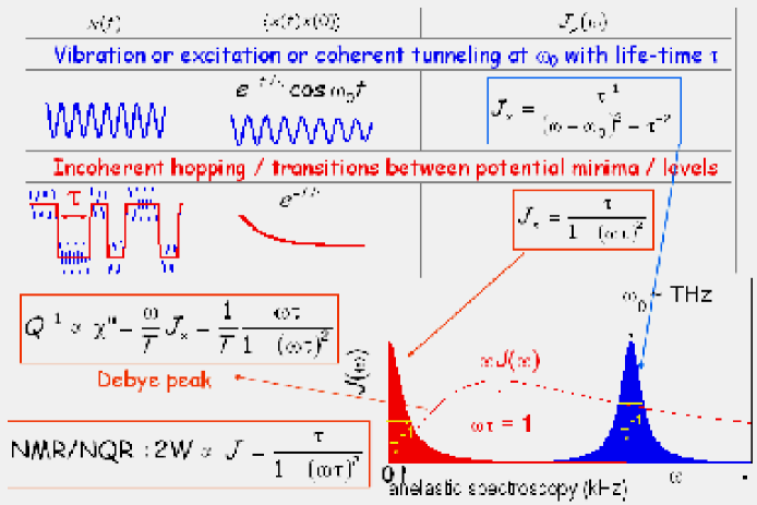
Figure 2-4: Spectral densities $J\left(\omega\right)$ of $x\left(t\right)$ for resonant (blue) and relaxational or diffusive (red) processes. The imaginary elastic compliance or energy loss is related to $J\left(\omega\right)$ through the fluctuation-dissipation theorem.

This is schematically shown in Fig. 2-4, where the physical quantity $x\left(t\right)$, e.g. atomic positions coupled to strain $\varepsilon$ and to the electric field gradient producing NQR relaxation (see Sec. 4.9), displays resonant and pseudodiffusive types of motion. The spectral density of the fluctuations of $x$ contains both the peak centered at $\omega_{0}>10^{12}$ s^-1 (local vibration in a potential minimum) and the central peak of width $\tau^{-1}$ (hopping between two potential minima with rate $\tau^{-1}$). At acoustic frequencies the resonant process has negligible spectral weight and only the central peak is observed; $s^{\prime\prime}$ can be obtained from Eq. (2.36), while the NQR relaxation rate is given directly by $J\left(\omega\right)$ [17].

2.3 Distributions of relaxation times

Up to now we considered anelastic relaxation from equivalent non-interacting elastic dipoles, all having the same relaxation time $\tau$, as is the case of very diluted solid solutions. More common are the situations with distributions of relaxation times $g\left(\tau\right)$, due to static disorder or interactions among the dipoles, which result in broader peaks in $s^{\prime\prime}\left(\omega,T\right)$.

In what follows we are mainly concerned with the imaginary or absorption part of the compliance or modulus, because it is easier to analyze than the real part. In fact, the imaginary part $s^{\prime\prime}\left(\omega,T\right)$ associated with a relaxation process with characteristic time $\tau$ is peaked around the temperature at which $\omega\tau\left(T\right)=1$ holds, and is superimposed over a background contribution $s_{\text{bkg}}^{\prime\prime}\left(\omega,T\right)$ which is usually small and slowly varying over the temperature range of the peak in $s^{\prime\prime}\left(\omega,T\right)$. Instead, the contribution to $s^{\prime}\left(\omega,T\right)$ extends well above the temperature for which $\omega\tau\left(T\right)=1$, and is superimposed to elastic compliance $s_{\text{el}}^{\prime}\left(T\right)$, which is large and temperature dependent. This is at variance with the dielectric case, where the equivalent of $s_{\text{el}}^{\prime}\left(T\right)$ is close to the vacuum permittivity $\varepsilon_{0}$.

2.3.1 Uniform distribution of activation energies or $\ln\tau$

The simplest distribution of relaxation times with a clear physical meaning is a uniform distribution in the activation energy $E$: $g\left(E\right)=\left(E_{2}-E_{1}\right)^{-1}$ for $E_{1}\leq E\leq E_{2}$. Setting $\ln\tau=\ln\tau_{0}+E/T$, this is equivalent to a uniform distribution in $\ln\tau$: $\ln\tau_{0}+E_{1}/T\leq$ $\ln\tau\leq$ $\ln\tau_{0}+E_{2}/T$:

$$g\left(E\right)dE=\frac{dE}{E_{2}-E_{1}}=\frac{d\left(\ln\tau\right)}{\ln\tau_{2}-\ln\tau_{1}}=g\left(\ln\tau\right)d\left(\ln\tau\right)$$ (2.38)

The imaginary part of the compliance can be easily integrated over such a distribution, where we include a relaxation strength $\propto 1/T$ [see Eq. (2.16)]:

$$s^{\prime\prime}\left(\omega,T\right) =\int_{E_{1}}^{E_{2}}\frac{dE}{\left(E_{2}-E_{1}\right)}\frac{\Delta s}{T}\frac{2\,\omega\tau_{0}e^{E/T}}{1+\left(\omega\tau_{0}e^{E/T}\right)^{2}}=$$

$$=\frac{2\Delta s}{\left(E_{2}-E_{1}\right)}\left[\arctan\left(\omega\tau_{0}e^{E_{2}/T}\right)-\arctan\left(\omega\tau_{0}e^{E_{1}/T}\right)\right]\,.$$ (2.39)

This distribution, however, usually provides a poor fit to very broadened processes, since it develops a plateau at the maximum. It has been used to describe glassy processes, by letting $\tau_{2}\left(T\right)$ diverge at the freezing temperature, and assuming a constant relaxation strength. The omission of the $1/T$ term in the relaxation strength transforms the broad plateau into a linear temperature increase from the freezing temperature up to the maximum at $\omega\tau_{2}\left(T_{m}\right)\simeq 1$, which describes reasonably well, for example, the dielectric maximum of some relaxor ferroelectrics [18], possibly by smoothing the cutoff at $\tau_{2}$ [19].

2.3.2 Fuoss-Kirkwood distribution

Fuoss and Kirkwood [20] showed that, when the imaginary part of a susceptibility $\chi^{\prime\prime}$ may be written as

$$\chi^{\prime\prime}\left(\omega\right)=\int_{0}^{\infty}d\left(\ln\tau\right)\,g\left(\ln\tau\right)\frac{\omega\tau}{1+\left(\omega\tau\right)^{2}}$$ (2.40)

then the distribution function $g$ of the relaxation times may be expressed by analytical continuation in terms of $\chi^{\prime\prime}$:

$$g\left(\ln\tau\right)=\frac{1}{\pi}\left[\chi^{\prime\prime}\left(-\ln\tau/\tau_{m}+i\frac{\pi}{2}\right)+\chi^{\prime\prime}\left(-\ln\tau/\tau_{m}-i\frac{\pi}{2}\right)\right]\,,$$ (2.41)

where $\tau_{m}=\omega^{-1}$ at the maximum of $\chi^{\prime\prime}$ is the mean value of $\tau$, when $g\left(\ln\tau\right)$ is even in $\ln\tau/\tau_{m}=$ $\ln\tau-\ln\tau_{m}$ and therefore $\chi^{\prime\prime}$ is even in $\ln\omega\tau_{m}$. In this manner, it is possible to associate a distribution function $g\left(\ln\tau\right)$ to any analytical form of broadened peak in $s^{\prime\prime}\left(\omega,T\right)$. A commonly used expression is

$$s^{\prime\prime}\left(\omega\right)=\frac{\alpha\left(\omega\tau\right)^{\alpha}}{1+\left(\omega\tau\right)^{2\alpha}}=\frac{\alpha}{2\cosh\left[\alpha\ln\left(\omega\tau\right)\right]}$$ (2.42)

with $0<\alpha\leq 1$; $\alpha=1$ corresponds to a Debye peak, whereas $\alpha<1$ broadens the peak by a factor $\alpha^{-1}$ in the $\ln\tau$ and therefore $T^{-1}$ scale (and lowers its amplitude by $\alpha$); the corresponding distribution, called Fuoss-Kirkwood distribution [8], can be calculated through eq. (2.41):

$$g_{\text{FK}}\left(\ln\tau\right) =\frac{1}{\pi}\left[\frac{\alpha}{2\cosh\left[-\alpha\ln\left(\tau/\tau_{m}\right)+i\alpha\frac{\pi}{2}\right]}{\small+}\frac{\alpha}{2\cosh\left[-\alpha\ln\left(\tau/\tau_{m}\right)-i\alpha\frac{\pi}{2}\right]}\right]=$$

$$=\frac{\alpha}{\pi}\frac{\cosh\left[\alpha\ln\tau/\tau_{m}\right]\cos\frac{\alpha\pi}{2}}{\cos^{2}\frac{\alpha\pi}{2}+\sinh^{2}\left[\alpha\ln\tau/\tau_{m}\right]}$$ (2.43)

and is normalized to 1; $g_{\text{FK}}\left(x\right)$ can also be well approximated with a Lorentzian

$$g_{\text{FK}}\left(x\right)\simeq\frac{\alpha}{\pi\cos\frac{\alpha\pi}{2}}\frac{\left(w/2\right)^{2}}{x^{2}+\left(w/2\right)^{2}}\,\,\text{with}\quad w=3.38\times\left(\alpha^{-1}-1\right)$$ (2.44)

for $\alpha$ down to $0.4$. If $\ln\tau=\ln\tau_{0}\exp\left(E/k_{\text{B}}T\right)$, and the effect of a distribution in the values of $\tau_{0}$ is neglected in comparison to those of $E$, then $g_{\text{FK}}\left(\ln\tau\right)$ can be attributed to a distribution in $E$, roughly Lorentzian with a temperature dependent full width at half maximum $w_{E}=3.38\times\left(\alpha^{-1}-1\right)k_{\text{B}}T$.

2.3.3 Cole-Cole distribution

The simple expression

$$\chi=\frac{1}{1+\left(i\omega\tau\right)^{\alpha}}\,,\quad\chi^{\prime\prime}=\frac{\left(\omega\tau\right)^{\alpha}\sin\left(\frac{\pi}{2}\alpha\right)}{1+\left(\omega\tau\right)^{2\alpha}+2\left(\omega\tau\right)^{\alpha}\cos\left(\frac{\pi}{2}\alpha\right)}=\frac{1}{2}\frac{\sin\left(\frac{\pi}{2}\alpha\right)}{\cosh\left[\alpha\ln\left(\omega\tau\right)\right]+\cos\left(\frac{\pi}{2}\alpha\right)}$$ (2.45)

is very popular in the analysis of the dielectric susceptibility. The corresponding distribution function is

$$g_{\text{CC}}\left(\ln\tau\right)=\frac{1}{2\pi}\frac{\sin\left(\pi\alpha\right)}{\cosh\left[\alpha\ln\left(\tau/\tau_{m}\right)\right]+\cos\left(\pi\alpha\right)}\,.$$ (2.46)

2.3.4 Other expressions

Other expressions for $\chi\left(\omega\right)$ and corresponding distributions in $g\left(\ln\tau\right)$ are used, especially in the dielectric literature, for example the Havriliak-Negami one,

$$\chi=\frac{1}{\left[1+\left(i\omega\tau\right)^{\alpha}\right]^{\gamma}}\,.$$ (2.47)

To my knowledge there are no particular physical reasons for preferring one over the others, except the empirical fact that different processes may be better interpolated by different expressions. For example, a process whose $\chi^{\prime\prime}\left(\omega,T\right)$ is not even in $1/T$ will be better interpolated by an expression of the Havriliak-Negami type, which is not even in $\ln\omega\tau$, but also a simpler expression, like

$$\chi^{\prime\prime}\left(\omega\right)=\frac{1}{\left(\omega\tau\right)^{\alpha}+\left(\omega\tau\right)^{-\beta}}$$ (2.48)

may be used [21]. The latter is a generalization of the Fuoss-Kirkwood expression, where rescaling in $1/T$ by $\alpha$ is adopted for the low-$T$/high-$\tau$ region and rescaling by $\beta$ in the high-$T$ region. An even more flexible expression was proposed by Jonscher [22],

$$\chi^{\prime\prime}\left(\omega\right)=\frac{1}{\left(\omega\tau_{1}\right)^{\alpha}+\left(\omega\tau_{2}\right)^{-\beta}}$$ (2.49)

where $\tau_{1}\left(T\right)$ and $\tau_{2}\left(T\right)$ are two relaxation times, possibly following the Arrhenius law, which describe the relaxation of the system at long and short times, respectively.

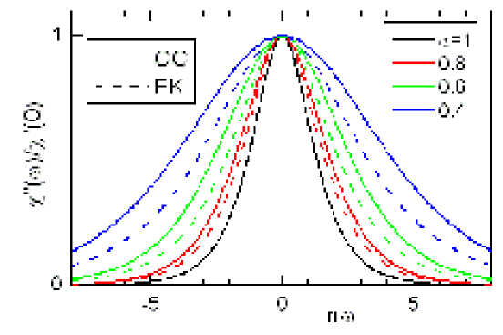
Figure 2-5: Normalized $\chi^{\prime\prime}$ vs $\ln\omega$ according to the Fuoss-Kirkwood and Cole-Cole expressions for different values of $\alpha$.

2.4 Interacting elastic dipoles

The treatment of interacting elastic dipoles is of particular importance in the case of oxygen in the CuO_x planes of YBCO, where the concentration of dipoles $0.1<x<1$ is by no means small, and their interaction is so strong to give rise to a complicated phase diagram. Under such conditions, any attempt at describing the anelastic relaxation from the hopping of the O atoms should somehow take into account their mutual interactions, which are both of electronic and elastic origin. The description of the structural phase diagram of YBCO, however, requires rather sophisticated models with asymmetric interactions (different along the $a$ and $b$ axes) at least up to the next-nearest neighbors (so-called ASYNNNI models [23]). Such models can be solved only with Monte Carlo techniques, and are generally adopted to reproduce the YBCO structural phase diagram, in only few cases to evaluate the oxygen diffusion coefficient [24, 25], and no attempt exists to evaluate the dynamic elastic compliance due to oxygen hopping. The numerical results on the tracer diffusion coefficient [24, 25] are of little help in analyzing the anelastic data.

Wipf and coworkers [26] carried out an analysis of the high temperature anelastic measurements of YBCO where the interaction between the O atoms is treated in the Bragg-Williams or mean-field approximation; in that manner, the complexity of the YBCO phase diagram cannot be obtained, since only a single ordering phase transformation is reproduced, identified with the tetragonal to orthorhombic one, but useful expressions of the dynamic compliance can be obtained. This treatment is particularly appropriate to the analysis of anelastic relaxation from oxygen jumps in the RuO_2-δ planes of Ru-1212, which can indeed be considered as a diluted solution of O vacancies with long range elastic interactions (see Sect 6.2).

A treatment of the dynamics of interacting elastic dipoles had also been carried out previously by Dattagupta [27, 28] in the mean field approximation, assuming that the actual elastic field that a particular dipole senses is substituted with a mean stress field $\sigma_{\text{MF}}$ due to all the other dipoles, the same for all dipoles. Such a treatment has also been reviewed in connection with the Snoek relaxation of O interstitial atoms in bcc metals [29]. Dattagupta’s model does not explicitly take into account the concentration of relaxing dipoles, since it assumes that there is one dipole per cell, which is able to change between three possible orientations; it is the elastic analogous of the Curie-Weiss theory of interacting magnetic dipoles, and the result is essentially the same. If the elastic interaction $E=\lambda\sigma_{\text{MF}}$ among the dipoles on the average favors parallel orientations of the major axis of $\lambda$, $\Delta E=E_{\perp}-E_{\parallel}>0$, a cooperative alignment of the dipoles occurs, which results in an increase of both the relaxation strength $\Delta\left(T\right)$ and relaxation time $\tau$ by a factor $\left(1-T_{\mathrm{C}}/T\right)^{-1}$. The effect of the cooperative motion can be roughly viewed as the coordinated motion of several dipoles instead of independent dipoles, which results in a larger effective elastic dipole, but also in a slower reorientation time. When the anisotropic component of the interaction energy, $\Delta E$, is of the order of the thermal energy $k_{\text{B}}T$, the dipoles start freezing into a fixed orientation, resulting in a ferroelastic ordering transition, similar to the ferromagnetic or ferroelectric one. The expression of $s^{\prime\prime}$ above $T_{\mathrm{C}}$ becomes

$$\frac{s^{\prime\prime}}{s^{\prime}} =\tilde{\Delta}\frac{\omega\tilde{\tau}}{1+\left(\omega\tilde{\tau}\right)^{2}}$$ (2.50)

$$\tilde{\Delta} =\frac{\Delta\left(T\right)}{1-T_{\mathrm{C}}/T}\propto\frac{T_{\mathrm{C}}}{T-T_{\mathrm{C}}}\,,\quad\tilde{\tau}=\frac{\tau\left(T\right)}{1-T_{\mathrm{C}}/T}$$ (2.51)

and, assuming $\Delta\left(T\right)=\Delta_{0}/T$ can be put in the form

$$\frac{s^{\prime\prime}}{s^{\prime}}=\frac{\Delta_{0}}{T}\frac{\omega\tau}{\left(1-T_{\text{c}}/T\right)^{2}+\left(\omega\tau\right)^{2}}$$ (2.52)

where $\tau$ is the relaxation time for non-interacting dipoles. Such a treatment might be adapted to only two orientations, as is the case of oxygen in YBCO, and the expressions of the elastic compliance and relaxation time might be extended below $T_{\mathrm{C}}$; the dependence on the dipole concentration $c$ might be taken into account as an interaction energy $\Delta E\simeq$ $\lambda\sigma_{\text{MF}}\propto$ $\left(\Delta\lambda\right)^{2}c$, giving rise to $k_{\text{B}}T_{\mathrm{C}}\simeq$ $\Delta E\propto c$, as also suggested in [27, 28]. However, the result would be correct only in the limit of low concentration, and in what follows I will adopt Wipf’s approach [26].

2.4.1 Ordering transition

Let us consider the CuO_x plane of YBCO, where, like the interstitial atoms in Fig. 2-1c, the O atoms can occupy sites of type 1 and 2, corresponding to the positions generally called O(1) and O(5) (see Fig. 5-1); in the completely ordered phase only sites of type 1 are occupied. The starting point of Wipf’s analysis [26] is the equilibrium condition for the O atoms between the sites of type 1 and 2:

$$\mu_{1}\left(c_{1},c,T\right)=\mu_{2}\left(c_{2},c,T\right)$$ (2.53)

where $\mu_{\alpha}$ is the chemical potential of the O atoms in the sublattice $\alpha$ and $c=\frac{x}{2}$ is the fraction of sites populated in the CuO_x plane ($0\leq c\leq 0.5$ for YBCO) with

$$c_{1}+c_{2}=c\,.$$ (2.54)

The chemical potentials are evaluated from the free energy $F=U-TS$, as

$$\mu_{\alpha}=\frac{\partial F}{\partial c_{\alpha}}$$ (2.55)

and in the Bragg-Williams approximation is $F=\overline{E}-k_{\text{B}}T\ln\mathcal{N}$, with $\overline{E}$ the average energy of the dipoles and $\mathcal{N}$ the number of ways a state with that energy may be obtained, disregarding the interactions among dipoles. Therefore, if the crystal contains $N$ cells, $\mathcal{N}$ is the number of ways $N_{1}$ O atoms can be put in $N$ sites of type 1 and $N_{2}$ O atoms in the other $N\;$sites of type 2:

$$\mathcal{N}=\frac{N\left(N-1\right)...\left(N-N_{1}+1\right)}{N_{1}!}\frac{N\left(N-1\right)...\left(N-N_{2}+1\right)}{N_{2}!}=\prod_{\alpha=1}^{2}\frac{N!}{N_{\alpha}!\left(N-N_{\alpha}\right)!}$$ (2.56)

and using Stirling’s formula $\ln N!\simeq N\ln N$ and $c_{\alpha}=N_{\alpha}/N$

$$-\ln\mathcal{N}=N\sum_{\alpha=1}^{2}\left[c_{\alpha}\ln c_{\alpha}+\left(1-c_{\alpha}\right)\ln\left(1-c_{\alpha}\right)\right]$$ (2.57)

The mean energy is

$$\overline{E}=\sum_{\alpha,\beta}\sum_{i,j<i=1}^{N}E_{ij}^{\alpha\beta}c_{\alpha}c_{\beta}$$ (2.58)

where in the mean-field approximation [28] the interaction energy between two dipoles of type $\alpha$ and $\beta$ in the cells $i$ and $j$ is set

$$E_{ij}^{\alpha\beta}=\left\{\begin{array}[c]{c}E_{\parallel}\quad\text{if }\alpha=\beta\\ E_{\perp}\quad\text{if }\alpha\neq\beta\end{array}\right.$$ (2.59)

yielding a mean energy per unit cell

$$\overline{E}=E_{\parallel}\sum_{\alpha}c_{\alpha}^{2}+E_{\perp}\sum_{\alpha}c_{\alpha}\left(c-c_{\alpha}\right)=\Delta E\sum_{\alpha}c_{\alpha}^{2}+E_{\perp}c^{2}$$ (2.60)

where

$$\Delta E=E_{\parallel}-E_{\perp}$$ (2.61)

and $\Delta E<0$ favors parallel orientations. The free energy per unit cell can then be written as

$$F=\overline{E}-k_{\text{B}}T\ln\mathcal{N}=\Delta E\sum_{\alpha}c_{\alpha}^{2}+E_{\perp}c^{2}+k_{\text{B}}T\sum_{\alpha=1}^{2}\left[c_{\alpha}\ln c_{\alpha}+\left(1-c_{\alpha}\right)\ln\left(1-c_{\alpha}\right)\right]$$ (2.62)

and the chemical potentials

$$\mu_{\alpha}=\frac{\partial F}{\partial c_{\alpha}}=2\Delta Ec_{\alpha}+k_{\text{B}}T\ln\left(\frac{c_{\alpha}}{1-c_{\alpha}}\right)$$ (2.63)

or, adopting the notation of [26],

$$\mu_{\alpha}=\frac{\partial F}{\partial c_{\alpha}}=-\alpha\left(c_{\alpha}-\frac{c}{2}\right)+k_{\text{B}}T\ln\left(\frac{c_{\alpha}}{1-c_{\alpha}}\right)$$ (2.64)

where the energy is referred to that of the completely disordered state, $c_{\alpha}=\frac{c}{2}$, and $\alpha=-2\Delta E>0$ is the difference in energy between states 1 and 2, supposed to be weakly dependent on temperature. By equating $\mu_{1}$ and $\mu_{2}$ we obtain

$$\frac{\alpha}{k_{\text{B}}T}\left(c_{1}-c_{2}\right)=\ln\left[\frac{c_{1}\left(1-c_{2}\right)}{c_{2}\left(1-c_{1}\right)}\right]$$ (2.65)

having solutions different from the trivial one $c_{1}=c_{2}=\frac{1}{2}$ only below the critical temperature

$$k_{\text{B}}T_{\mathrm{C}}=\alpha\frac{c}{2}\left(1-\frac{c}{2}\right)\,;\;$$ (2.66)

below $T_{\mathrm{C}}$, the equation can be solved numerically for $c_{1}$, as shown in Appendix A.

2.4.2 Coupling to stress and relaxation strength

On application of a stress $\sigma_{kl}$, the elastic energy of each O atom of type $\alpha$ changes by

$$-v_{0}\lambda_{kl}^{(\alpha)}\sigma_{kl}\,,$$ (2.67)

where for tetragonal elastic dipoles $\lambda_{xx}^{(1)}=\lambda_{yy}^{(2)}=\lambda_{1}\,,\quad\lambda_{yy}^{(1)}=\lambda_{xx}^{(2)}=\lambda_{2}$, while the $z$ component has no interest since it is the same for both types of sites, so that the anelastic strain due to the oxygen dipoles is (compare with Eq. (2.24))

$$\varepsilon_{xx}=-\varepsilon_{yy}=\frac{1}{2}\left(c_{1}-c_{2}\right)\left(\lambda_{1}-\lambda_{2}\right)\,.$$ (2.68)

The change in elastic energy, given by Eq. (2.9), results in a change of the populations from $c_{\alpha}\$to $c_{\alpha}^{\prime}\left(\sigma\right)$ such that

$$\mu_{1}\left(c_{1}^{\prime},c,T\right)-v_{0}\lambda_{kl}^{(1)}\sigma_{kl}=\mu_{2}\left(c_{2}^{\prime},c,T\right)-v_{0}\lambda_{kl}^{(2)}\sigma_{kl}$$ (2.69)

and expanding to first order in $c_{\alpha}^{\prime}-c_{\alpha}$ and using the fact that $\left(c_{1}^{\prime}-c_{1}\right)=-\left(c_{2}^{\prime}-c_{2}\right)$,

$$c_{1}^{\prime}-c_{1}=\frac{v_{0}\left(\lambda_{kl}^{(1)}-\lambda_{kl}^{(2)}\right)\sigma_{kl}}{\frac{\partial\mu_{1}}{\partial c_{1}}+\frac{\partial\mu_{2}}{\partial c_{2}}}=\frac{v_{0}\left(\lambda_{1}-\lambda_{2}\right)\left(\sigma_{xx}-\sigma_{yy}\right)}{\frac{\partial\mu_{1}}{\partial c_{1}}+\frac{\partial\mu_{2}}{\partial c_{2}}}$$ (2.70)

which results in an anelastic strain

$$\varepsilon_{xx}^{\text{an}}=-\varepsilon_{yy}^{\text{an}}=\frac{1}{2}\left[\left(c_{1}^{\prime}-c_{2}^{\prime}\right)-\left(c_{1}-c_{2}\right)\right]\left(\lambda_{1}-\lambda_{2}\right)=\frac{v_{0}\left(\lambda_{1}-\lambda_{2}\right)^{2}\left(\sigma_{xx}-\sigma_{yy}\right)}{\frac{\partial\mu_{1}}{\partial c_{1}}+\frac{\partial\mu_{2}}{\partial c_{2}}}$$ (2.71)

or relaxation of the compliances $\delta s_{ijkl}=\varepsilon_{ij}^{\text{an}}/\sigma_{kl}$:

$$\delta s_{11}=\delta s_{22}=-\delta s_{12}=\frac{v_{0}\left(\lambda_{1}-\lambda_{2}\right)^{2}}{\frac{\partial\mu_{1}}{\partial c_{1}}+\frac{\partial\mu_{2}}{\partial c_{2}}}=F_{1}\left(T\right)\frac{v_{0}\left(\lambda_{1}-\lambda_{2}\right)^{2}}{k_{\text{B}}T}$$ (2.72)

where the factor $F_{1}\left(T\right)$ is computed from eq. (2.64):

$$F_{1}\left(T\right)=\left[\frac{1}{8}\left[\frac{c\left(2-c\right)}{c_{1}\left(1-c_{1}\right)}+\frac{c\left(2-c\right)}{c_{2}\left(1-c_{2}\right)}\right]-\frac{T_{\mathrm{C}}}{T}\right]^{-1}$$ (2.73)

For $T>T_{\mathrm{C}}$ it is $c_{1}=c_{2}=c/2$ and therefore

$$F_{1}\left(T\right)=\frac{T}{T-T_{\mathrm{C}}}\quad\left(T>T_{\mathrm{C}}\right)$$ (2.74)

and $\delta s$ becomes the Curie-Weiss susceptibility; below $T_{\mathrm{C}}$, $F_{1}\left(T\right)$ falls off to zero, as shown in Fig. 2-6.

2.4.3 Relaxation rate

Following [26], the rate equation for the instantaneous out-of-equilibrium concentrations $c_{1}^{\prime\prime}$ and $c_{2}^{\prime\prime}=c-c_{1}^{\prime\prime}$ is

$$\frac{dc_{1}^{\prime\prime}}{dt} =\frac{1}{2}\tau_{0}^{-1}\exp\left(-E_{0}/k_{\text{B}}T\right)\left[c_{2}^{\prime\prime}\left(1-c_{1}^{\prime\prime}\right)e^{\Delta E/2k_{\text{B}}T}-c_{1}^{\prime\prime}\left(1-c_{2}^{\prime\prime}\right)e^{-\Delta E/2k_{\text{B}}T}\right]$$ (2.75)

$$=\frac{1}{2\tau}\left[c_{2}^{\prime\prime}\left(1-c_{1}^{\prime\prime}\right)e^{\alpha\left(c_{1}^{\prime\prime}-\overline{c}\right)/k_{\text{B}}T}-c_{1}^{\prime\prime}\left(1-c_{2}^{\prime\prime}\right)e^{-\alpha\left(c_{1}^{\prime\prime}-\overline{c}\right)/k_{\text{B}}T}\right]$$

where $\tau^{-1}=\tau_{0}^{-1}\exp\left(-E_{0}/k_{\text{B}}T\right)$ is the relaxation rate when sites 1 and 2 are equivalent (absence of stress and disordered state), the two terms are the rates from 1 to 2 and vice versa, taking into account the probability that the neighboring site is empty, while the $e^{\pm\Delta E/2k_{\text{B}}T}$ factors account for the non-equivalence introduced by the ordering transition, where the difference in the site energies is given by the difference in chemical potential, without counting the entropic term:

$$\Delta E=E_{2}-E_{1}=\alpha\left(c_{1}^{\prime\prime}-c_{2}^{\prime\prime}\right)=2\alpha\left(c_{1}^{\prime\prime}-\overline{c}\right)\,.$$ (2.76)

On setting $dc_{1}/dt=0$ one finds again eq. (2.65), which demonstrates the consistence between the thermodynamic-statistical and the kinetic analyses.

In order to find the dynamic response to a small applied stress, we set $c_{1}^{\prime\prime}=c_{1}+\delta c$ and $c_{2}^{\prime\prime}=c_{2}-\delta c$ into the rate equation, where $\delta c\left(t\right)$ is the small response to the applied stress, and keep terms to the first order in $\delta c$; after some algebra one obtains

$$\frac{d\delta c}{dt}=-\frac{\delta c}{\tau_{\text{eff}}}$$ (2.77)

with

$$\tau_{\text{eff}}=\tau\frac{\frac{c}{2}\left(1-\frac{c}{2}\right)}{\sqrt{c_{1}c_{2}\left(1-c_{2}\right)\left(1-c_{1}\right)}}F_{1}\left(T\right)=\tau\,F_{2}\left(T\right)\,.$$ (2.78)

For $T>T_{\mathrm{C}}$ the factor before $F_{1}$ becomes unity, and one finds that

$$\tau_{\text{eff}}=\tau\frac{T}{T-T_{\mathrm{C}}}\quad\left(T>T_{\mathrm{C}}\right)$$ (2.79)

which represents the critical slowing down on approaching the phase transformation. The functions $F_{1}$ and $F_{2}$ that enhance the relaxation strength and time near $T_{\mathrm{C}}$ are shown in Fig. 2-6.

Figure 2-6: $F_{1}$ and $F_{2}$ versus reduced temperature for $c=0.4$.

Chapter 3 Experimental

3.1 The samples

The YBa₂Cu₃O_6+x (YBCO), La_2-xSr_xCuO₄ (LSCO) and Nd₂CuO_4+δ (NCO) samples have been prepared by M. Ferretti at the Department of Chemistry and Industrial Chemistry of the University of Genova, Italy. The powders of the starting oxides were mixed in appropriate amounts and calcined, typically 1233 K in air for 6 h for YBCO, 1323 K for 18 h for LSCO and 90 h for NCO. The powders were then pressed into bars $5\times 5\times 50$ mm³ and sintered in fluent O₂ (typically YBCO at 1253 K for 22 h and LSCO at 1323 K for 18 h), and further oxygenated in fluent O₂ at lower temperature for the case of YBCO. The powders were checked with X-ray diffraction for impurity phases from decomposition or incomplete solid state reaction, and sometimes intermediate grinding and sintering treatments were made. Especially RuSr₂GdCu₂O₈ (Ru-1212) required a long processing route [30] before the final oxygenation at 1343 K in fluent O₂ for one week, followed by cooling at 50 K/h.

The ingots were finally cut with a circular diamond saw to the dimensions suitable for the anelastic measurements: length of $40-50$ mm, thickness of $0.2-1.5$ mm, width of $4-5$ mm. The samples were rather porous (from 10% up to 50% for Ru-1212) and some of the oil used during cutting remains in the pores and it is almost impossible to completely remove it with solvents (toluene and acetone) in a ultrasound bath. The complete removal of the oil can be accomplished by burning it, heating the sample at high temperature. The residual oil, which can also be adsorbed from the pumping system [31], has a freezing transition around 220 K giving rise to an absorption peak and anomalies in the elastic moduli (see also Sect 5.7).

Further characterization of the samples was made by measuring the resistivity and superconducting transition with a four-probe technique with a closed cycle cryocooler from 300 down to 12 K. Checks were made that resistivity $\rho$ did not depend on the amplitude and direction of the applied voltage. The oxygen stoichiometry in YBa₂Cu₃O_6+x was estimated by combined analysis of the $\rho\left(T\right)$ curves (compared with literature data) and of the anelastic spectra; in some cases series of samples have been prepared with different stoichiometries, checked by iodometric titration and from the cell parameters from X-ray diffraction.

3.2 Anelastic measurements with resonating samples

The equation of the vibration of a solid near one of its resonances is that of a damped harmonic oscillator with resonance frequency [8] $f_{0}=\alpha\sqrt{M/\rho}=$ $\frac{{}^{\omega_{0}}}{2\pi}$ where $M$ is an effective elastic modulus and $\alpha$ a geometrical factor depending on the vibration mode. Then, the equation of motion for strain under application of a stress $\sigma_{0}e^{i\omega t}$ with $\omega\simeq\omega_{0}$ is

$$\sigma_{0}e^{i\omega t}=\alpha^{2}\left(M^{\prime}+iM^{\prime\prime}\right)\,\varepsilon+\rho\ddot{\varepsilon}=\rho\omega_{0}^{2}\left(1+i\tan\phi\right)\varepsilon-\rho\omega^{2}\varepsilon$$ (3.1)

where the real and imaginary parts of the modulus have been introduced.

All measurements presented here have been made by exciting the samples on their 1st, 3rd and 5th flexural modes. Thanks to the sample dimensions, with length $30-800$ times larger than the thickness, and to the low vibration amplitude, always within the linear regime, the approximation of simple bending of thin bars is a good one. Under such approximation the modulus involved in the flexural vibrations is the Young’s modulus $E$, that relates uniaxial stress and strain of a long sample of uniform cross section. In the case of pure extensional vibrations, where stress and strain obey $\sigma=E\varepsilon$ all over the sample, the resonance frequency of the $n$-th mode is given by $f_{n}=\left(n/2l\right)\sqrt{E/\rho}$ where $l$ and $\rho$ are the sample length and density (neglecting a correction factor that takes into account the finite size of the cross-section with respect to the length and proportional to the square of Poisson’s ratio [32]). In the case of flexure, strain is inhomogeneous along the sample thickness, passing from extension on the convex side to compression on the concave one, as shown in Fig. 3-1. The effective modulus (the real part) is therefore $E$, but reduced of a geometrical factor taking into account the sample cross section; for the fundamental mode of a thin bar of thickness $h$, it is [8]

$$f=1.03\frac{h}{l^{2}}\sqrt{E/\rho}\,;$$ (3.2)

the frequencies of third and fifth modes are respectively 5.40 and 13.3 times larger.

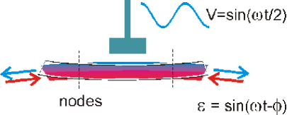
Figure 3-1: Electrostatic excitation of the flexural vibrations of a thin bar. Strain is inhomogeneous along the sample thickness: from a uniaxial expansion (blue) to a compression (red).

We never tried to estimate the absolute value of $E$ because of irregularities in the samples shapes and above all due to the large sample porosity (from 10 to 50%), but it is possible to measure the variation of $E\left(T\right)$ with respect to a reference temperature $T_{0}$ through

$$\frac{E\left(T\right)}{E\left(T_{0}\right)}=\frac{f^{2}\left(T\right)}{f^{2}\left(T_{0}\right)}\,,$$ (3.3)

where the temperature dependence of $\rho\left(T\right)$ is neglected in comparison to that of $E\left(T\right)$.

The elastic energy loss can be measured with two methods. In the free decay method, the excitation is switched off and, according to Eq. (3.1) with $\sigma_{0}=0$, the vibration amplitude falls off as

$$\varepsilon\left(t\right)=\varepsilon_{0}e^{i\omega_{0}\sqrt{1+i\tan\phi}\,t}\simeq\varepsilon_{0}e^{i\omega_{0}t}e^{-\phi\,\omega_{0}t/2}.$$ (3.4)

Therefore, interpolating with a straight line the logarithm of the vibration amplitude $A\left(t\right)=\varepsilon_{0}\exp\left(-\phi\,\omega_{0}t/2\right)$, $\log\left[A\left(t\right)/A\left(0\right)\right]=-\frac{1}{2}Q^{-1}\omega_{0}t$, it is possible to deduce $\tan\phi=Q^{-1}$. This method is useful when the decay constant $Q/(\pi f_{0})$ is long enough to let the amplitude decay to be recorded.

For larger dissipations or frequencies the forced oscillation method can be used, where the vibration amplitude is measured on sweeping frequency near resonance. From Eq. (3.1), the vibration amplitude is

$$\left|A\right|^{2}=\frac{\left(\sigma_{0}/\rho\right)^{2}}{\left(\omega_{0}^{2}-\omega^{2}\right)^{2}+\omega_{0}^{4}\tan^{2}\phi}$$ (3.5)

and by least square fitting of $A^{-2}\left(\omega^{2}\right)$ one obtains the resonance frequency $\omega_{0}/2\pi$ and the elastic energy loss coefficient $Q^{-1}$.

3.3 The anelastic relaxation setup

The anelastic measurements were based on resonant sample techniques developed in the Laboratory of Solid State Acoustics at the Istituto di Acustica ”O. M. Corbino” of CNR, starting from Prof. P. G. Bordoni up to Profs. G. Cannelli and R. Cantelli. The sample is suspended on thin thermocouple wires in correspondence with the nodal lines for the flexural vibrations; generally the nodes at $0.225l$ from the sample ends ($l=$ sample length) are used, since they are very close to nodes of both the 1st and 5th flexural modes, whose resonance frequencies are in the ratio 1:13.3. It is therefore possible to measure these two frequencies during the same run.

As schematically shown in Fig. 3-1, an electrode is kept very close the sample surface and the sample, if not conducting, is covered with silver paint in correspondence with the electrode and suspension wires, in order to have electrical continuity and proper grounding (through one of the thermocouple wires). An excitation ac voltage $V_{\text{exc}}$ is applied to the electrode with frequency $f/2$ and amplitude up to 200 V; this induces a potential of opposite sign on the surface of the sample and the resulting electrostatic force $\propto V_{\text{exc}}^{2}$ excites vibrations of the sample at frequency $f$ (100 Hz-100 kHz depending on the sample shape and vibration mode). These vibrations modulate the sample/electrode capacitance, which is part of a high frequency ($\sim 10$ MHz) circuit, and therefore modulate its resonant frequency, which is in turn demodulated with a coupled resonating circuit with tunable capacitance. This revelator, called vibrometer, was constructed in the Solid State Acoustics Laboratory by Profs. Nuovo and Bordoni. I improved the data acquisition by introducing a lock-in amplifier that measures the signal amplitude and can detect low vibration levels at high noise level, and developed the acquisition software. Now it is routine to perform measurements at several frequencies during the same run sometimes in semiautomatic manner. This is very important whenever the status of the sample is modified by the measurement itself, for example due to oxygen loss in vacuum at high temperature, and a subsequent run at a different frequency could not be compared with the previous one for making an analysis at different frequencies. If the sample is properly mounted and its intrinsic dissipation is $Q^{-1}\sim 10^{-4}$ or larger, it is possible to measure several flexural and torsional modes with the same mounting; Fig. 2-3 is an example with 1st, 3rd and 5th flexural modes vibrating at 1.3, 7.2 and 18 kHz respectively.

There are two separate inserts for low (1-300 K) and high temperature (100-950 K) measurements, evacuated by a diffusion pump; He exchange gas is used for thermalization, and an adsorption pump is used at low temperature, in order to minimize the adsorption by the sample of residual gases when the diffusion pump is closed (being cooled with liquid N₂, the adsorption pump does not condense the He exchange gas).

The low temperature insert has a cylindrical brass cell that can be closed both with a conical coupling with vacuum grease to the flange or with In wire for measurements below 2 K. The cell is equipped with heater and silicon diode for temperature control and a wound copper tube for the flow of LHe. The whole insert may be closed with a vacuum tight glass dewar and works as a LN bath cryostat and LHe flow or bath cryostat: below 5 K the dewar is filled with LHe and may be pumped in order to lower temperature down to 1.1 K. The thermocouple is Au-0.003Fe versus chromel.

The high temperature insert is made of stainless steel and ceramic insulating parts and is closed with a quartz tube. Temperature is regulated with a tubular furnace or dewar with LN.

3.4 Reliability of the anelastic spectroscopy measurements

Sometimes, there is scepticism on interpretations of anelastic relaxation processes outside mechanisms based on atomic defects, dislocations, domain boundaries and grain boundaries; in addition, it is often felt that the anelastic spectroscopy should be particularly sensitive to the polycrystalline nature of ceramic samples and to grain boundaries, making the interpretation of the anelastic spectra very unreliable. In this section few arguments are put forward demonstrating that such doubts are generally unjustified.

Regarding the effect of impurity phases, generally found at the grain boundaries, it should be remarked that anelastic spectroscopy probes the whole volume of the sample; therefore, if defects motions or phase transformations occur in an impurity phase, their effect will be weighted with the molar fraction of the phase (and another factor of order unity taking into account the different moduli of bulk and impurity phase [33]). Therefore, spurious phases may affect the anelastic spectra exactly as they affect other bulk measurements like specific heat or neutron spectroscopy, and much less than techniques sensitive to the grain surfaces, like resistivity, dielectric susceptibility or optical spectroscopies. In the samples considered here the molar fraction of impurity phases did never exceed few percents, as checked by X-ray diffraction, which means that their possible contribution to the anelastic spectrum was rather small. Of course, if the impurity phase presents a phase transformation, even small amount of it may produce noticeable effects on the anelastic spectrum, as for example occurs with La_1-xCa_xMnO₃ samples containing Mn₃O₄ below the detection limit with standard powder X-ray diffraction [33]. The only cases considered here of little characterized anomalies looking like phase transformations are those in YBCO around 240 K (Sec. 5.7) and 120-160 K (Sec. 5.5.1), but even in these cases, their peculiar dependence on oxygen doping strongly suggest mechanisms involving the CuO_x planes of YBCO.

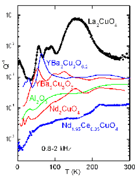
Figure 3-2: Elastic energy loss versus tempertaure of ceramic samples of LSCO, YBCO, NCCO at various dopings and of porous alumina, measured in the same conditions at frequencies between 0.8 and 2 kHz.

A convincing indication against the contribution of impurity phases and also against instrumental contributions to the spectra examined in the present study is the strong dependence of these spectra on doping and the fact that they are completely different for different families of cuprates. This is shown in Fig. 3-2, comparing the $Q^{-1}\left(T\right)$ curves of ceramic samples of La_2-xSr_xCuO₄, YBa₂Cu₃O_6+x and Nd_2-xCe_xCuO_4+δ at various dopings, measured in the same conditions exciting the mode at lower frequency, between 0.8 and 2 kHz. All the samples were prepared in the same laboratory by M. Ferretti and coworkers, with the same equipments and procedures, except for sintering times and temperatures, but the spectra are completely different from each other. The fact that there is no single feature that is shared among all the spectra excludes the influence of systematic instrumental effects. The only possible instrumental contribution is from freezing of adsorbed oils around 220 K, as discussed in Sec. 5.7, but the curve of Nd_1.95Ce_0.05CuO₄ sets the upper limit of this possible contribution to a value too small to affect the spectra of LSCO and YBCO; in addition, a sample of Al₂O₃ with 50% porosity, also shown in Fig. 3-2, does not present any anomaly at that temperature, in spite of being much more susceptible to oil uptake. The influence of gases adsorbed by the samples is discussed in Sec. 5.5.1. The lack of peaks common to all the curves in Fig. 3-2 excludes the influence of a spurious phase like copper oxides, certainly absent in the almost flat and very low $Q^{-1}\left(T\right)$ curve of Nd_1.95Ce_0.05CuO₄. The same observation is made by varying doping within the same cuprate family, as shown in Fig. 3-3 for LSCO. In this figure, there is a progressive change of the spectrum with increasing $x$, indicating that all the features depend on doping of La_2-xSr_xCuO₄ and therefore not on spurious phases. If they contributed to one of the peaks labeled T or S or to the maximum at LHe temperature, they should exist also at $x=0.2$, where instead the elastic energy loss is $2-3$ orders of magnitude smaller (except for the step at the structural transformation from cubic to tetragonal, shifted down to 80 K at such doping).

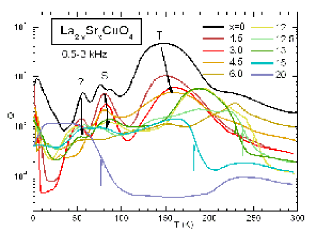
Figure 3-3: Anelastic spectra of La_2-xSr_xCuO₄ at various doping levels $x$ in %; the vertical coloured arrows indicate the structural transitions from cubic to tetragonal.

In Fig. 3-3, the only instance in which there is no clear smooth evolution of the curves with doping is the double peak at 80 K for $x=0$, which should not be identified with peak S in the Sr-doped samples (see Sec. 4.11.3). The curve with $x=0$ was measured after a rather strong outgassing treatment that possibly introduced O vacancies in the CuO₂ planes (see Sec. 4.8.3), and the double peak might be related to such vacancies. The peak at 50 K also appears as some doping dependent relaxation in La_2-xSr_xCuO₄, but it is labeled with a question mark since we were not able to find a plausible mechanism for it, and it will not be discussed in this Thesis.

Finally, the possibility that the motion of grain boundaries itself may contribute to the present measurements can be excluded; this type of relaxation, in fact, requires the diffusion of the cations, which occurs at temperatures comparable to the sintering temperatures, above 1200 K. Instead, all the thermally activated relaxation processes observed here at high temperature are clearly related to diffusion of nonstoichiometric oxygen.

3.5 The UHV system for sample treatments

The oxygenation and some of the outgassing treatments were made in a Ultra High Vacuum (UHV) system realized by Ing. Dalla Bella at RIAL Vacuum (Parma, Italy) after my project. It consists of a main spherical chamber with Bayard-Alpert head and Residual Gas Analyzer, pumped by turbomolecular, ionic and Ti sublimation pumps. Two CF63 flanges on opposite sides connect on one side, through an all-metal gate valve, another chamber connected with the gas inlet line, capacitive heads and a quartz tube flanged CF63 where the sample is put for the treatments. On the other side, the spherical chamber is connected to a chamber for introducing the sample without breaking vacuum in the rest of the system, equipped with a magnetically coupled rotary-linear feedthrough with a tray for depositing the sample. The trail has the possibility of some lateral movement and is surrounded by stainless steel wire, so that with a rotary movement it is possible to retrieve also fragile samples, generally wrapped with Pt wire for protection and for avoiding direct contact with the quartz tube. The sample is heated up to 1100 ^oC by a horizontal tubular furnace mounted on wheels.

The gas inlet line consists of a multiway valve connecting to various pure gas bottles (O₂, H₂, D₂, N₂), and a bakeable all metal section with inlet and outlet needle valves, a small (17.3 cm³) and a large (200 cm³) calibrated volumes and capacitance head, in order to be able to admit a known amount of gas.

The base vacuum before any treatment was in the $10^{-9}$ mbar range, but could be improved with baking to the $10^{-10}$ mbar range in particular cases.

Chapter 4 LSCO

La_2-x(Sr/Ba)_xCuO₄ (LSCO or LBCO) is the first high-$T_{\mathrm{C}}$ superconductor discovered by Bednorz and Müller. Having $T_{\mathrm{C}}\leq 40$ K, it is not particularly attractive for applications, but has the simplest structure among the superconducting cuprates and is probably the best characterized. Doping may be achieved both through excess oxygen in La₂CuO_4+δ and by partial substitution of La³⁺ with Sr²⁺ or Ba²⁺; in the latter case, if excess oxygen is completely removed, one does not have the complications due to the ordering of the nonstoichiometric oxygen, which characterize the other HTS cuprates.

4.1 Structural phase diagram

LSCO is formed by layers of CuO₆ octahedra intercalated by (La/Sr) atoms, as shown in Fig. 4-1. The substitution $x$ trivalent La ions with divalent Sr or Ba introduces $p=x$ holes/unit cell in the CuO₂ layers, which form a conducting band. Interstitial oxygen (O${}_{\text{i}}$) can also be introduced in tetrahedral coordination with four apical O atoms and four La atoms; each O^2- provides two conducting holes. A small amount of excess O ($\delta\sim 10^{-3}$) is present in as-prepared La₂CuO_4+δ and can be increased to few percent by equilibrating in O₂ at moderate temperatures [34]; up to 12% O${}_{\text{i}}$ can be introduced by electrochemical oxidation [35, 36]. By increasing the Sr doping, the equilibrium concentration of O${}_{\text{i}}$ decreases, and electrochemical oxidation is necessary to obtain La_2-xSr_xCuO_4+δ.

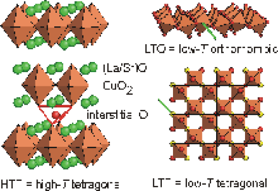
Figure 4-1: Structure of LSCO. Left panel: ideal HTT structure; the O atoms (not shown) are at the vertices of the octahedra; also shown is an interstitial O atom and its tetrahedric coordination with the nearest neighbor apical O atoms. Right panel: the two more stable tilt patterns of the octahedra, giving rise to the LTO and LTT structures; in the latter case, adjacent layers of the octahedra are rotated by 90^o, so that the overall structure is tetragonal.

4.1.1 Tolerance factor and Low-Temperature Orthorhombic (LTO) phase

When decreasing temperature, the equilibrium bond lengths in the (La/Sr)O layers decrease faster than the equilibrium CuO bond length within the CuO₂ planes, and the resulting lattice mismatch is relieved by a buckling of the CuO₂ planes [37] below a temperature $T_{t}(x)$. This phenomenon is typical of the perovskite structure, formed by a three-dimensional network of BO₆ octahedra intercalated by A cations. In the ideal cubic case, which is the high temperature structure of most perovskites, the ratio of the A-O and B-O bond lengths is $l_{\text{A-O}}/l_{\text{B-O}}=\sqrt{2}$, and it is usual to define a tolerance or Goldschmidt factor

$$t=\frac{l_{\text{A-O}}}{\sqrt{2}l_{\text{B-O}}}\,,$$ (4.1)

which is 1 in the ideal cubic case, and, when becomes $<1$, indicates that the size of the BO₆ octahedra is too large for the equilibrium A-O bond length, resulting in rotations of the octahedra. In many cases, the transitions of perovskites from cubic to lower symmetries involving rotations of the octahedra are understood in terms of $t$ decreasing with temperature.

Figure 4-2: Perovskite structure with evidenced the A-O and B-O bonds, whose lengths in the ideal cubic structure are in the ratio $\sqrt{2}$.

The same reasoning can be applied to the perovskite layers of La_2-xSr_xCuO₄, defining the tolerance factor [37]

$$t=\frac{l_{\text{La-O}}}{\sqrt{2}l_{\text{Cu-O}}}\,.$$ (4.2)

Since the octahedra are relatively rigid units, the buckling results in a collective tilting of the octahedra, and the structure changes from high-temperature tetragonal (HTT) to low-temperature orthorhombic (LTO, see Figs. 4-1 and 4-4a).

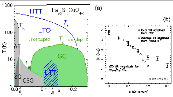
Figure 4-3: (a) Structural (blue), magnetic (gray) and electric (green) phase diagram of LSCO. AF = antiferoomagnetic, SG = spin glass, CSG = cluster spin glass, SC = superconducting. (b) average and local tilt angle of LTO phase versus doping (Ref. [38]).

Doping reduces the mismatch between LaO blocks and CuO₂ planes in two ways i) substitution of La³⁺ with larger Sr²⁺ or insertion of interstitial O expand the lattice, and therefore relieve the compressive stress on the CuO₂ planes; ii) doping holes in the CuO₂ planes removes charge from the CuO antibonds, therefore shortening them [35, 39]. Therefore, the HTT phase is stabilized by doping, and $T_{t}\left(x\right)$ is an almost linearly decreasing function of $x$, as appears from the LSCO phase diagram in Fig. 4-3. In the same figure is also reported the average tilt angle $\theta$ in the LTO phase from diffraction measurements, again a decreasing function of doping; the decrease seems to be much more regular at a local level, as found by extracting the pair-distribution functions (PDF) from neutron diffraction [38], and prosecutes into the HTT phase, which therefore should consist of disordered tilted instead of untilted octahedra.

4.1.2 Other tilt patterns and the Low-Temperature tetragonal (LTT) phase

Actually, other tilt patterns besides the LTO one are possible, all describable in terms of a rotation axis of the octahedra within the $ab$ plane, and therefore in terms of two rotation angles $Q_{1}$ and $Q_{2}$ about two orthogonal axes within $ab$. Such axes are generally chosen at 45^o with the Cu-O bond directions (the direction of the $a$ axes of the LTO cell, while the $a$ and $b$ axes of the HTT cell is parallel to the Cu-O bonds) [40, 41], as shown in Fig. 4-4a.

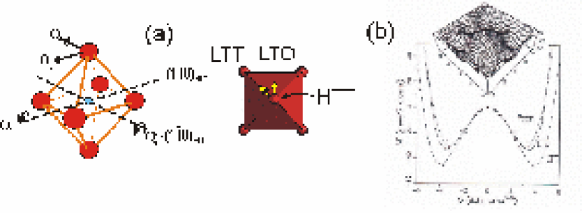
Figure 4-4: (a) The possible tilts of the CuO₆ octahedra in LSCO; (b) calculated local potential for an octahedron in LBCO, with eight minima corresponding to LTT and LTO tilts (Ref. [42]).

The two variants of the LTO phase are then described by $\left(Q_{1},0\right)$ and $\left(0,Q_{2}\right)$, while the LTT phase by $\left|Q_{1}\right|=\left|Q_{2}\right|$. The intermediate cases $Q_{1}\neq$ $Q_{2}\neq$ 0 are also possible, and produce intermediate phases, generally precursors to the LTT one [41, 43, 44]. Tilt patterns intermediate between LTT and LTO are present also within the twin boundaries in the LTO phase. Such twins walls have been observed to be nucleation sites for the LTT phase [45].

The LTT structure is stable only at low temperature, near the doping $x=1/8$, and if there is sufficient disorder in the ionic sizes in the La sublattice. The latter is obtained by substituting La with Ba instead of Sr, which has a still larger radius [46] (the radii of 12-fold coordinated Ba²⁺, Sr²⁺ and La³⁺ are 1.61, 1,44 and 1.36 Å), or by doping with Sr²⁺ and substituting part of La³⁺ with the larger Nd³⁺.

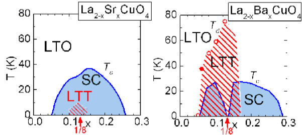
Figure 4-5: Low-temperature region of the phase diagram of LSCO and LBCO, with the different regions of stability of the LTT structure below $T_{t}$. The open circles are $T_{t}$ from Ref. [40], while the closed one from the measurement of Fig. 4-10 .

Figure 4-5 shows the region of stability of the LTT phase for La${}_{2-x}M_{x}$CuO₄ with $M=$ Sr, Ba, deduced from various types of measurements [40, 47]. It appears also that the LTT phase is associated with a depression of the superconducting $T_{\mathrm{c}}$.

It is important to note that in the LTO phase all the O atoms in the CuO₂ planes are equivalent, while in the LTT phase one can distinguish between the O atoms on the rotation axes, and therefore remaining on the plane, and those shifted out of the plane; this provides a modulation of the potential felt by the charge carriers, which results in a mutual stabilization of the LTT modulation and of the static hole stripes (see Sec. 4.4), whose spacing becomes commensurate with the lattice spacing at $x=\frac{1}{8}$.

The local potential felt by each octahedron free to tilt has been theoretically found to have eight minima in correspondence of the four possible LTO and four LTT tilts separated by barriers $E/k_{\text{B}}\sim 300-500~{}$K [42, 48] (see Fig. 4-4b).

4.2 Electric phase diagram

The electric and magnetic phase diagram of LSCO can be considered as representative of the other cuprates, except for complications arising from the O nonstoichiometry in the latter.

As anticipated above, the concentration of holes doped in the CuO₂ planes of La_2-xSr_xCuO_4+δ is $p=x+2\delta$, neglecting clustering of O${}_{\text{i}}$ (see Sec. 4.8). The transport properties (conductivity, Hall coefficient, dielectric permittivity) of lightly doped La_2-xSr_xCuO_4+δ can be understood in terms of conventional semiconductor physics [49, 50, 51]: La₂CuO₄ has static dielectric constant $\varepsilon=310$, and the hole effective mass is $m_{h}=2m_{e}$. The holes are thermally ionized from the acceptors, to which are bound with an energy $E_{b}$(Sr) $=$ $10-20$ meV for the case of Sr dopants and $E_{b}$(O) $\sim$ 31 meV for O${}_{\text{i}}$. Conduction is of band-type at high temperature, namely $\sigma\propto$ $p\propto$ $\exp(-E_{b}/kT)$ at $T>70~{}$K, and variable-range-hopping below 50 K ($\sigma\propto$ $\exp[-(T_{0}/T)^{1/4}]$).

For $p>0.05$ the planes start to superconduct below $T_{\mathrm{c}}\left(p\right)$, which has a maximum versus doping at $p_{\text{opt}}\simeq 0.15$ (see Figs. 4-3 and 4-5); the system is called underdoped, optimally doped and overdoped, depending on the value of $p$ with respect to $p_{\text{opt}}$. Underdoped cuprates exhibit various anomalies, partly interpreted in terms of opening of pseudogaps in the charge or spin excitations and partly in terms of charge stripes; the latter will be dealt with in some detail in Sect 4.4. In overdoped cuprates, instead, a uniform metallic state sets in and becomes so stable that superconductivity eventually disappears.

In cuprates of the LSCO family, a depression of superconductivity occurs in correspondence with the formation of the LTT phase, and this is understood in terms of locking of the charge stripes to the LTT lattice modulation, as explained in Sect 4.4.

4.3 Magnetic phase diagram

The study of the superconducting and magnetic phase diagram of the CuO₂ planes of the superconducting cuprates is a complex and fascinating subject (for a review see e.g. [17]), but I will mention only the issues relevant to the anelastic measurements. In the absence of doping, the CuO₂ planes are semiconducting, with Cu in the Cu²⁺ oxidation state having spin $s=\frac{1}{2}$; these spins order antiferromagnetically (AF) below the Néel temperature $T_{\text{N}}=315$ K, with the staggered magnetization within the $ab$ plane, and mainly parallel to $b$. There is also a small component of the spins pointing out of the planes, due to the small tilt of the Cu-O bases of the octahedra; this weak canting produces a ferromagnetic component that dominates the low frequency magnetic susceptibility [52]. Doping holes causes some Cu atoms to pass into the Cu³⁺ state with $s=0$, and this disturbs the AF order; in La_2-xSr_xCuO₄ $T_{\text{N}}\left(x\right)$ drops to 0 K already at the critical doping $x_{c}\simeq\,0.02$ (see Fig. 4-3).

A model of how the holes disturb the AF order has been proposed by Gooding et al. [53], starting from the hypothesis that at low temperature and low doping the holes are localized near the Sr dopants. The ground state for one isolated hole would be doubly degenerate with the hole circulating either clockwise or anticlockwise over the four Cu atoms nearest neighbors to the Sr atom. The hole motion couples to the transverse fluctuations of the Cu spins and produces a spiraling distortion of the AF order within the $ab$ plane; at this point it should be noted that the model assumes the staggered magnetization of the hole-free plane along $c$, while in fact it is along $b$, but the model may help in focusing some mechanisms responsible for the magnetic phase diagram of the HTS cuprates. The ground states with disordered distributions of Sr impurities would consist of AF correlated domains delimited by the Sr atoms and with the in-plane AF order parameter randomly oriented, resulting in a (cluster) spin-glass state. The domains would be separated by narrow domain walls with disordered spins and ferromagnetic character which connect the Sr atoms. The hole mobility is much higher in FM rather than AFM regions (the hopping of a hole in a AF domain requires also a spin flip, if destruction of AF order has to be avoided), and therefore with increasing temperature and doping the holes move along these domain walls, which would therefore correspond to the charge stripes of the next Section.

Whatever model is chosen, experiments probing the local spin fluctuations, like NQR [17, 50] and $\mu$SR [54], indicate that the spin degrees of freedom associated with the doped holes are different from the in-plane Cu²⁺ spin degrees of freedom that order themselves below $T_{\text{N}}$, and the localization of the doped holes allows the associated spins to progressively slow down and freeze [17, 50]. For $x<x_{c}$ one has long range AF order below $T_{\text{N}}$, and the doped spins freeze into a spin glass (SG) state below $T_{f}\left(x\right)\$linearly increasing with $x$ (see Fig. 4-3). For $x>x_{c}$ there is no long range AF order and approaching $T_{g}\simeq 0.2$ K$/x$ AF correlations develop within domains separated by hole-rich walls, and with easy axes uncorrelated between different clusters, giving rise to a cluster spin-glass (CSG) state (see Fig. 4-3).

More recent neutron scattering experiments [55] of the magnetic correlations in La_2-xSr_xCuO₄ for $x<x_{c}$ suggests a different picture of the spin glass phase, with the 3D AF ordered phase coexisting below $\sim 30$ K with domains of the stripe phase observed for $x>x_{c}$ (see also next Section). It has been proposed that the hole localization starting around 150 K involves an electronic phase separation into regions with $x_{1}\sim 0$ and $x_{2}\sim 0.02$, and the volume fraction of the $x_{2}=0.02$ phase changes as a function of the Sr doping, in order to achieve the average $x$.

4.4 Hole stripes

A phenomenon that seems to be common to many superconducting cuprates, and has been attracting enormous interest, is the segregation of the conducting holes into stripes, while maintaining very good conductivity or even superconductivity [56, 57, 58, 59, 17, 2]. The literature on the subject is vast, and I will deal only with those aspects related to the anelasticity. On the theoretical side, it is debated whether these charge stripes compete against superconductivity [3] or on the contrary they are an essential ingredient of HTS [5, 6]. In both cases, an important issue is the dynamics of the transverse fluctuations of these stripes, which has been modeled in terms of collective pinning from the doping impurities by C. Morais Smith [60]. To my knowledge, the only experimental results on the low frequency stripe fluctuations are the anelastic measurements presented here [61, 62, 63, 64, 65].

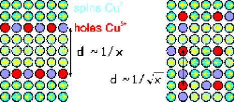
Figure 4-6: Left: ordered stripes with periodicity $d$ commensurate with the lattice at $x=\frac{1}{8}$. The holes (Cu³⁺ with spin $s=0$) are in red, while the violet sites along the hole stripes do not have a definite spin direction, since they are also walls between different AF domains. Right: possible situation if the holes were uniformly distributed.

The first indications of segregation of the charge carriers into stripes came from measurements of the correlation length $\xi\left(x\right)$ for the AF order in LSCO, deduced from $T_{\text{N}}\left(x\right)$ [66] and from NQR experiments [17]: the observation is that the increase of $\xi$ on cooling is limited to a length $l\sim a/x$ ($a$ is the lattice constant). Since the AF correlations can develop only over regions free holes (which have $s=0$ instead of $\frac{1}{2}$), $l$ should represent the size of domains free of holes and, if the holes were uniformly distributed over the CuO₂ plane, their separation should scale as $l\sim a/\sqrt{x}$, while $l\sim a/x$ indicates that the holes are in one-dimensional walls of fixed hole density separating hole-free domains or stripes (see also Fig. 4-6). Note that these charge stripes are not charge-density waves, having a much sharper modulation and allowing the Cu²⁺ spins to form AF domains between in the charge-poor regions.

Several other indirect indications of the existence of the charge stripes have been found [17, 67], including the observation of inhomogeneous Cu-O bond lengths in the CuO₂ planes with probes of the local structure like EXAFS [4] and pair-distribution functions (PDF) from neutron diffraction [68]. The strongest evidence of the existence of parallel magnetic and charge stripes comes from magnetic inelastic neutron diffraction, which reveals one-dimensional dynamic charge and magnetic correlations with a spacing $d$ incommensurate with the lattice parameter and decreasing with doping as $d\propto 1/x$ [69]. In addition, the direction of the modulation changes from diagonal to parallel with respect to the Cu-O bonds when increasing doping above $x=0.055$, which also separates the semiconducting from the superconducting region [59, 70]. These correlations are observable also as static structural modulations in the region of the phase diagram $x\simeq\frac{1}{8}$ with the LTT phase stabilized by partial substitution of La with Nd [56, 57]. In fact, at $x=\frac{1}{8}$ the stripe spacing becomes commensurate with the lattice, and the LTT tilt pattern provides a modulation to which the stripes are locked. The situation for $x=\frac{1}{8}$ deduced from neutron diffraction is represented in the left hand of Fig. 4-6. The hole stripes act as antiphase boundaries between regions where the Cu²⁺ spins have AF correlation; varying doping does not modify the hole density within a charge stripe, which remains 0.5, but only the stripe separation (hence $d\propto 1/x$). It is also found that, on cooling, the formation of the charge stripes precedes that of the AF spin stripes [56].

4.5 Nd_2-xCe_xCuO_4+δ

The structure of La₂CuO₄, also called T structure [71], is one of three possible structures of A₂BO₄. Nd_2-xCe_xCuO₄, instead, presents the so-called T’ structure, where the cations and the O atoms of the CuO₂ planes are in the same positions as in the T structures, while the O atoms in the (Nd/Ce)O blocks correspond to the interstitial sites of La₂CuO_4+δ; on the other hand, the interstitial positions in the T’ structure correspond to the apical O atoms in the T structure. The correspondence between the oxygen positions in the two structures is shown by the arrows in Fig. 4-7. The result of this shift in the oxygen positions is that there are no short Cu-O bonds along the $c$ axis and therefore no CuO₆ octahedra, but only flat CuO₂ planes.

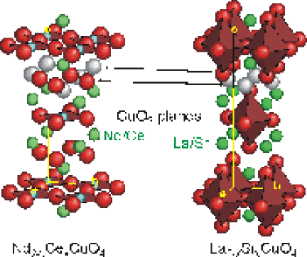
Figure 4-7: Comparison between the T (LSCO) and T ’ (NCCO) structures. The arrows indicate the correspondence between the O interstitial positions (white) in one structure and O in the NdO or LaO blocks in the other one.

It should be mentioned that Nd₂CuO₄ supports only electron doping (substituting Nd³⁺ with Ce⁴⁺), at variance with all the other superconducting cuprates.

4.6 The anelastic spectrum

The anelastic spectrum of LSCO contains several relaxation processes whose intensity and appearance strongly depend on the type and level of doping. Figure 4-8 present the elastic energy loss and Young’s modulus between 1 and 800 K of stoichiometric semiconducting La₂CuO₄ and Nd₂CuO₄. It should be stressed that as-prepared La₂CuO_4+δ has $\delta\sim 0.003$ that drastically modifies the anelastic spectrum, and the result of Fig. 4-8 is obtained after accurate outgassing of the excess oxygen. Nd₂CuO₄ appears like a normal solid without defects or excitations: the absorption is low and the elastic modulus decreases regularly by less than 20% between 0 and 800 K. Stoichiometric La₂CuO₄ is also free of defects, in principle, but its anelastic spectrum presents extremely intense anomalies. The main difference between the two compounds is that Nd₂CuO₄ has flat CuO₂ planes while La₂CuO₄ has CuO₆ octahedra unstable against tilting (see Sec. 4.1 and Fig. 4-7). In fact, almost all the anelastic processes in La₂CuO₄ are due to some type of motion of the octahedra. Starting from high temperature we find (the numbers are those in Fig. 4-7): 1) the transformation from HTT to LTO structure; 2) motion of the domain walls between the two LTO variants (orthorhombic $b$ axis along $x$ or $y$); 3) octahedra tilt waves of solitonic type with thermally activated dynamics; 4) local tilts with dynamics governed by tunneling and interaction with the charge excitations; 5) thermally activated fluctuations of the charge stripes whose interaction with the lattice is mainly mediated by the octahedral tilts.

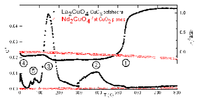
Figure 4-8: Elastic energy loss and Young’s modulus of La₂CuO₄ (500 Hz) and Nd₂CuO₄ (800 Hz) from 1 to 800 K.

Apart from the well known structural HTT/LTO transformation, all the other processes have been revealed by the anelastic experiments presented in the next Sections.

4.7 Structural phase transitions

4.7.1 HTT/LTO transformation and determination of the Sr content from $T_{t}$

The acoustic anomalies connected with this transformation have been studied by other authors [72, 73] and, in view of the polycrystalline nature of our samples, I did not attempt any quantitative analysis of the huge elastic anomaly and the accompanying rise in acoustic losses (#1 in Fig. 4-8). I only observe, together with Lee, Lew and Nowick [72], that only the region at $T>T_{t}$ may be analyzed in terms of Landau free energy, as in Ref. [73], because below $T_{t}$ the motion of the walls between the two possible LTO variants is predominant both in the imaginary and real moduli. The motion of the walls is very sensitive to defects like O${}_{\text{i}}$ and Sr, and is difficult to be modeled; their effect is to mask in most cases the cusps or kinks that would otherwise be observed in the moduli, making difficult even to establish where $T_{t}$ exactly is.

In the present Thesis the main interest in analyzing the HTT/LTO transition is for an accurate determination of the actual concentration of Sr and an estimate of its homogeneity. In fact, the transition temperature $T_{t}$ is strongly dependent on doping [74]

$$T_{t}\left(x\right)=\left(1-x/0.217\right)\times 535~{}\text{K ,}$$ (4.3)

and the width of the modulus step provides an upper limit to the possible inhomogeneities in $x$ over a sample, or, at least, by comparing widths of different $E\left(T\right)$ curves it is possible to tell whether a particular sample appears to be more inhomogeneous than the others.

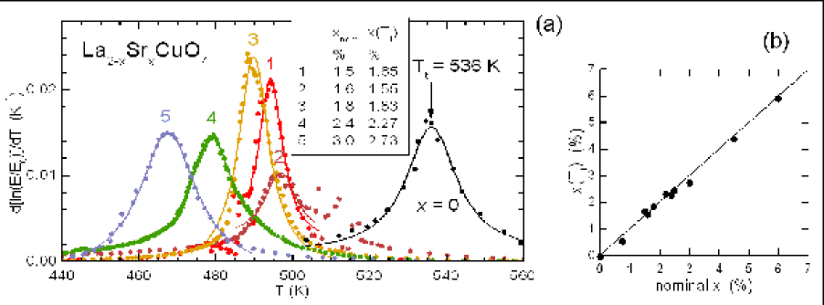
Figure 4-9: (a) Derivative of the relative variation of the Young’s modulus of La_2-xSr_xCuO₄ at the HTT/LTO transition at various values of $x$. (b) Sr content deduced from $T_{t}$ versus nominal $x$.

As mentioned above, there is no model available for fitting the $Q^{-1}\left(T\right)$ and $E\left(T\right)$ curve; as a uniform criterion to extract $T_{t}\,$from the anelastic spectra, I chose to identify $T_{t}$ with the inflection point of $E\left(T\right)$. In practice I fitted the derivative of the relative variation of the Young’s modulus, $d\ln\left[E/E\left(0\right)\right]/dT$, with lorentzian peaks, as in Fig. 4-9a, obtaining $T_{t}$ from the temperature of the maximum, and a transition width $\Delta T_{t}$ from the peak width. The method seems to work, since the curve for $x=0$ has a maximum exactly at $535$ K and the fitting Lorentzian at 536 K, as expected from Eq. (4.3) (it should be mentioned that sometimes distorted shapes of $E\left(T\right)$ have been measured on La₂CuO_4+δ, possibly connected with the presence of O${}_{\text{i}}$). The Sr concentrations estimated in this manner for the samples investigated here are plotted against the nominal $x$ in Fig. 4-9b, and show a good agreement. The relationship between transition width and inhomogeneity of the Sr concentration cannot be simply deduced by translating the peak width $\Delta T$ into $\Delta x$, since there is a considerable intrinsic width of the transition (critical softening above $T_{t}$ and domain wall motion below). This is particularly evident by observing that the curve for $x=0$, where $\Delta x=0$, is about twice broader than those for $x\sim 0.015$. It is seen, however, that transition #2 is broader than the others at similar doping, suggesting homogeneity problems with that sample.

4.7.2 LTO/LTT transformation

As anticipated in Sec. 4.1.2, extended domains of LTT phase can be found only in LBCO or Nd-substituted LSCO near $x=\frac{1}{8}$. The signature of the LTO/LTT transformation in the anelastic spectrum has been identified as a small acoustic absorption peak and stiffening below the transition temperature $T_{t}$ [47]. Figure 4-10 presents the Young’s modulus curves normalized to the value extrapolated to $T=0$ K for samples where La is substituted with 3% and 6% Sr and Ba.

Figure 4-10: Young’s modulus of LSCO and LBCO at $x=0.03$ and 0.06. $T_{g}$ indicates the CSG freezing temperature, and $T_{t}$ the onset of the LTO/LTT transition.

The only clear indication of formation of LTT phase is for the 6% Ba sample, below $T_{t}$ $\simeq 40$ K; such a stiffening is compatible with the ultrasonic measurements on LBCO with $0.10\leq x\leq 0.16$ [47] and with the available phase diagram [40, 75], as shown in Fig. 4-5.

Also LSCO at $x=0.06$ exhibits similar weak anomalies, which suggest a tendency to the formation of LTT domains also in LSCO, in accordance with high-resolution diffraction experiments [76]. In LSCO, however, such domains should be either confined to the twin boundaries or fluctuating, extremely small, and without long range correlation; instead, in LBCO and LSCO co-doped with Nd the diffraction experiments reveal a stable phase with long range order, which can also provide a pinning potential for the stripes. The anelastic experiments do not provide any direct information on the extension or topology of the LTT domains, and the elastic anomalies are likely connected with the domain boundaries. It is therefore possible that narrow domains of minority LTT phase in LSCO, with a high perimeter to area ratio, and extended LTT domains in LBCO produce elastic anomalies of comparable amplitude.

4.8 Interstitial oxygen

In literature extensive reports can be found on La₂CuO_4+δ that is heavily doped by electrochemical methods, generally enough to become superconducting. The interest in these researches is on electrical and structural phase separation and various types of ordering of O${}_{\text{i}}$ that occur under those conditions. My research is instead focused on the low concentration limit. Under normal conditions, the amount of excess oxygen in La₂CuO_4+δ is very small: by electrochemical reduction it has been estimated $\delta\sim 0.005$ in the as-prepared state [77, 78]; many estimates of $\delta\sim 0.01-0.02$ have also been reported, but, in view of the results presented in Sec. 4.8.2, I think that $\delta\lesssim 0.005$ is a more reliable evaluation.

Figure 4-11a presents the effect of outgassing La₂CuO_4+δ at progressively higher temperatures in vacuum starting from the as prepared state. Initially, two peaks labelled O1 and O2 are present at 225 and 300 K (at 300 Hz). Outgassing in vacuum reduces the intensity of these peaks in favor of another peak, labeled T, at 150 K. It is obvious to assign O1 and O2 to interstitial O, which is known to be present in small quantities in the sites indicated in Fig. 4-1, and is lost in vacuum at high temperature [79]. The hypothesis is confirmed by following the O₂ partial pressure during heating at 6 K/min in dynamic vacuum in a UHV system [34]; $p_{\text{O}_{2}}$ starts increasing above 550 K, indicating the loss of interstitial O, as also explained in Sec. 4.8.2.

The phenomenology is confirmed in Fig. 4-11b with another sample equilibrated at 900 K in partial pressures of O₂ ranging from 0.1 to 820 torr [80]. Each oxygenation was preceded by an outgassing at 700-750 ^oC, in order to obtain an initial reference state; the sample was then equilibrated at 620 ^oC for 90-120 min in a static atmosphere of pure O₂ and rapidly cooled.

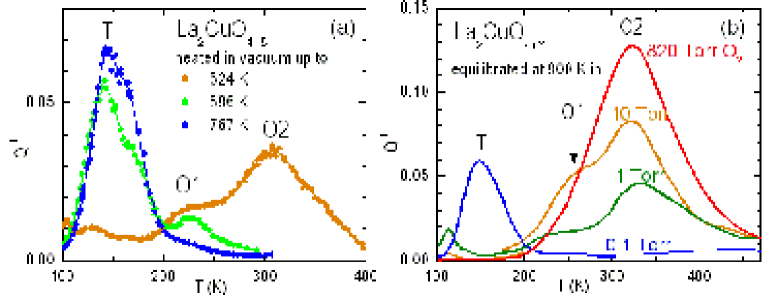
Figure 4-11: Dependence of the anelastic spectrum of La₂CuO_4+δ on $\delta$ (a) outgassing an as prepared sample at progressively higher temperatures in vacuum (300 Hz); (b) equilibrating at 900 K at different O pressures (800 Hz).

Figure 4-12 presents a fit to the $Q^{-1}\left(T\right)$ curves after equilibration in 10 torr with two Fuoss-Kirkwood peaks, Eq. (2.42), excluding the region at the right of the dashed lines, where contributions from the structural transition and the DW motion are important. The fitting parameters are $\tau_{0}=$ $2\times 10^{-14}$ s , $E_{\text{O1}}/k_{\text{B}}=6000$ K and $\alpha=0.4$ for peak O1 and $\tau_{0}=$ $8\times 10^{-14}$ s , $E_{\text{O2}}/k_{\text{B}}=7000$ K and $\alpha=0.5$ for peak O2.

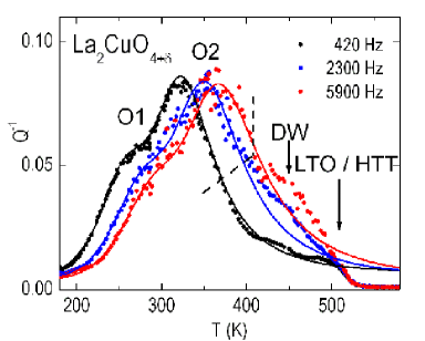
Figure 4-12: Anelastic spectrum of La₂CuO_4+δ in the region of the peaks due to hopping of isolated (O1) and paired (O2) interstitial O atoms. The curves are a fit of the data at the left of the dashed lines.

The most likely explanation for peak O1 and O2 is that O1 is due to hopping of isolated O${}_{\text{i}}^{2-}$ and O2 to pairs of O${}_{\text{i}}$, possibly peroxyde complexes with lower oxidation state, as suggested by the dependence of $\delta$ on the oxygen pressure (see Sec. 4.8.2). This hypothesis explains the fact that peak O1, expected to increase linearly with $\delta$, is rapidly overwhelmed by O2, which should increase with $\delta^{2}$. The parameter $\tau_{0}^{-1}$ of peak O1 is of the order of magnitude of the local phonon modes promoting the atomic jumps, and the resulting rate $\tau^{-1}\left(T\right)$ agrees with the observation that the excess oxygen becomes immobile below 140-150 K [81]: in that temperature range the estimated mean time $\tau$ between subsequent jumps passes from 5 min to more than 1 hour. It should be mentioned that experiments based on the analysis of the time and temperature dependence of the superconducting properties, which in turn depend on the ordering of O${}_{\text{i}}$ [81], provide activation enthalpies different from $E_{\text{O1}}$. Those experiments, however, determine the characteristic time of a complex process, like the aggregation of oxygen into domains and the possible ordering within the domains, while peak O1directly probes the hopping rate for single O${}_{\text{i}}$ defects.

Two features of peaks O1 and O2 seem at first at odds with a mechanism based on jumps of O${}_{\text{i}}$: the fact that they are very broad and that they shift in temperature with increasing doping. The broad width can be justified by the strong interaction between excess oxygen and the tilts of the surrounding octahedra, as discussed in the next Section. The network of these octahedra with their easy tilting modes provides a disordered environment for excess oxygen and mediates the interaction between the interstitial atoms much more effectively than in a regular lattice. In fact, at lower values of $\delta$ peak O1 is narrower (e.g. $\alpha=0.7$ for the intermediate curve of Fig. 4-11a [80]). This could also explain the shift of peak O1 to higher temperature with increasing $\delta$ in terms of correlated and therefore slower dynamics of O${}_{\text{i}}$.

These results can be compared with similar measurements made by Kappesser et al. [82], where only one thermally activated peak was observed, which was attributed to oxygen diffusion. Since that peak was found after electrochemical doping to $\delta=0.013$ and $\delta=0.035$, it should correspond to peak O2, with O1 possibly masked as in the highest curve of Fig. 4-11b. The peak temperature is close to that of O2 at a similar frequency, but the attempt frequency and activation enthalpy were estimated to be rather low: $\tau_{0}^{-1}=6.5\times 10^{8}~{}$s and $H/k_{\text{B}}=3600$ K.

4.8.1 The structure of the interstitial oxygen defect

The interstitial sites O(i) for O${}_{\text{i}}$ have been determined by neutron diffraction [83, 84, 36] and are shown in Figs. 4-1 and 4-13a. In the HTT structure and in the absence of ordering into superstructures they are at the center of regular tetrahedra formed by the neighboring apical oxygen atoms, O(a), with O(a)-O(i) distances in the range $1.6\div 2.2$ Å, and larger regular tetrahedra formed by La atoms. Inspection of Fig. 4-13a shows that all the interstitial sites for oxygen in the ideal HTT structure are equivalent from the elastic point of view. In fact, by symmetry the elastic dipole of O${}_{\text{i}}$ in the red site must have principal axes $z\parallel c$ and $x$ and $y$ within the $ab$ plane, parallel to the horizontal edges of the tetrahedron; the tetrahedron corresponding to the neighboring green site is rotated by 90^o about the $c$ axis with respect to the red one, but it may be also be obtained from it by inversion. This means that also the elastic dipole of O${}_{\text{i}}$ in the green sites may be obtained by inversion of the red one, and therefore the principal axes $x$ and $y$ must be equivalent; then, the strain due to O${}_{\text{i}}$ is isotropic within the $ab$ plane and there is no change of the elastic dipole for jumps of O${}_{\text{i}}$ in the ideal HTT structure.

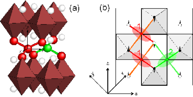
Figure 4-13: (a) two interstitial O atoms in the HTT structure; b) interstitial sites for O in the LTO structure labeled as 1 or 2 depending whether the shorter distance with the surrounding apical O atoms is along $\left(1\overline{1}0\right)$ or $\left(110\right)$. The white (black) circles are the apical O(a) atoms above (below) the plane of the O(i) sites; the arrows show their shift with respect to the ideal tetragonal HTT structure. The octahedra below O(i) are shadowed. The elastic dipoles due to the interstitial O atom are represented as ellipsoids with major axis along the shorter O(i)-O(a) distances.

In the LTO structure, where the anelastic relaxation peaks are observed, the octahedra are tilted about the $a$ axis (of the LTO representation). Figure 4-13b shows a top view of three interstitial sites (red and green circles) and the surrounding apical O atoms, with their displacements with respect to the tetragonal structure. The black circles are O(a) below the plane of O(i), with the corresponding octahedra shaded in gray, while the white circles are O(a) above it. The sites are labeled as 1 (red) or 2 (green) depending whether the O(i)-O(a) distances are shorter along $\left(1\overline{1}0\right)$ (or $x$) or along $\left(110\right)$ (or $y$). After the insertion of an O atom, the lattice will expand in different ways along the directions of the shorter bonds with respect to the longer bonds. In the figure is represented the case in which the O(a) which are closer are more displaced outwards (but in the case of the formation of a short peroxide bond the opposite can be true): the elastic dipole, represented as an ellipse, has the major axis along the direction of the shorter bonds and reorients by 90${}^{\text{o}}$ when the O atom jumps to a site of different type, modulating the $\varepsilon_{6}$ strain and giving rise to anelastic relaxation of the $c_{66}$ elastic constant.

The anisotropy of the elastic dipole in the $ab$ plane arises from the deviation of the LTO structure with respect to the HTT one, and therefore is expected to depend on temperature and doping. In fact, the tilt angles of the octahedra decrease continuously with doping, at least in La_2-xSr_xCuO_4+δ [85]; in addition, the orthorhombicity of La₂CuO_4+δ, defined as $\left(b-a\right)/a$, varies from 0.0165 at $\delta=0$ to 0.0119 in the oxygen-rich phase [36, 86].

From Fig. 4-13b it also appears that only jumps along $a$ contribute to anelastic relaxation, because they involve a rotation by 90^o of the anisotropic elastic dipole, while jumps in the $b$ direction do not. The hopping rates in the two directions may also be different, as discussed in more detail in Ref. [80], but up to now there are no experimental indications in this sense.

4.8.2 Dependence of $\delta$ on the O₂ pressure at high temperature

Under normal conditions, the amount of excess oxygen in La₂CuO_4+δ is very small: by electrochemical reduction it has been estimated $\delta\sim 0.005$ in the as-prepared state [77, 78], but no systematic data exist of the equilibrium values of $\delta$ as a function of temperature and pressure (the $p\delta T$ phase diagram). For this reason, I studied the absorption of interstitial O and the formation of O vacancies in La₂CuO_4+δ in equilibrium with O₂ pressures between $10^{-4}$ and $10^{3}$ torr or in vacuum at high temperature, in the UHV system described in Sec. 3.5 [34]. Such a study could be done in a more straightforward manner with a thermobalance; therefore I will omit the complications arising from measuring the amount of O absorbed or lost in a closed volume [34] and will concentrate on the results and the implications on the aggregation and valence state of excess oxygen in La₂CuO_4+δ.

Two different temperature regions are found: below about 600$~{}^{\text{o}}$C the equilibrium down to very low pressures of O₂ involves only interstitial oxygen atoms with negligible influence of O vacancies (V${}_{\text{O}}$), while above 700$~{}^{\text{o}}$C large amount of vacancies are created.

I determined the equilibrium values of $\delta$ as a function of pressure at 550$~{}^{\text{o}}$C, and in view of the very low amount of oxygen absorbed ($\delta<0.01$), it seems appropriate to initially suppose that O${}_{\text{i}}$ dissolves as O^2- ions, with the charge balance guaranteed by the change of the valence of Cu from Cu²⁺ to Cu³⁺ (La³⁺ does not support mixed valence). The reaction involved in the equilibrium between gaseous O₂ and interstitial O${}_{\text{i}}^{2-}$ can then be written as

$$\frac{1}{2}\text{O}_{2}+2\text{Cu}^{2+}\longleftrightarrow\text{O}_{\text{i}}^{2-}+2\text{Cu}^{3+}$$ (4.4)

and at equilibrium the concentrations must satisfy the mass action law

$$K=\frac{\left[\text{O}_{\text{i}}^{2-}\right]\,\left[\text{Cu}^{3+}\right]^{2}}{p^{1/2}\,\left[\text{Cu}^{2+}\right]^{2}}\,,$$ (4.5)

where $K\left(T\right)$ is the reaction constant and the square brackets represent the molar concentrations, assumed to be $\ll 1$. Introducing the neutrality condition, $\left[\text{Cu}^{3+}\right]=2\left[\text{O}_{\text{i}}^{2-}\right]=2\delta$, and the fact that for $\delta\ll 1$ it is $\left[\text{Cu}^{2+}\right]\simeq 1$, one obtains

$$\delta\propto p^{1/6}\text{.}$$ (4.6)

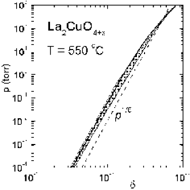
Figure 4-14: The experimental $\delta$ after equilibration at 550 ^oC in a pressure $p$ of O₂ is within the gray region; the continuous line is a fit with Eq. ( 4.10 ) and $a=0.003$, $b=0.02$.

The experimental $\delta\left(p\right)$ relationship is the gray region in Fig. 4-14 and shows deviation from $\delta\propto p^{1/6}$ already at $\delta\sim 0.002$. A transition to $p^{1/n}$ laws with $n=4,3,2$ could result from the formation of peroxide species like O${}_{\text{i}}^{-}$ or neutral interstitial O; for example, the formation of neutral O${}_{\text{i}}$ involves the reaction $\frac{1}{2}$O${}_{2}\longleftrightarrow$O${}_{\text{i}}$ with the equilibrium condition $K=$ $\delta/p^{1/2}$ instead of Eq. 4.5

Peroxide species are indeed found in La₂CuO_4+δ [35, 87], but at much higher doping levels; on the other hand, the anelastic spectra of Fig. 4-11 clearly show that interstitial O forms two distinct species already at $\delta\ll 0.01$; there are also indications that the second species consists of pairs of interstitial O atoms stabilized by partially covalent bonds with one of the neighboring apical O atoms. These peroxide complexes can be indicated as O${}_{\text{2i}}^{2-}$ in the equations for the chemical equilibrium, since involve two interstitial O atoms, and the reaction for their formation is

$$\text{O}_{2}+2\text{Cu}^{2+}\longleftrightarrow\text{O}_{\text{2i}}^{2-}+2\text{Cu}^{3+}\text{.}$$ (4.7)

We introduce the notation $c_{1}=\left[\text{O}_{\text{i}}^{2-}\right]$, $c_{2}=2\left[\text{O}_{\text{2i}}^{2-}\right]$, $h=\left[\text{Cu}^{3+}\right]$, which yield $\delta=c_{1}+c_{2}$ and the neutrality condition

$$h=2c_{1}+c_{2}\text{.}$$ (4.8)

The equilibria between gaseous O₂ and O${}_{\text{i}}^{2-}$ (Eq. 4.5) and between gaseous O₂ and O${}_{\text{2i}}^{2-}$ can be written as

$$K =\frac{c_{1}h^{2}}{p^{1/2}}$$ (4.9)

$$K^{\prime} =\frac{\left(c_{2}/2\right)h^{2}}{p}\,.$$

which yield

$$c_{1} =K^{1/3}\frac{p^{1/6}}{\left(2+\frac{2K^{\prime}}{K}p^{1/2}\right)^{2/3}}$$

$$c_{2} =\frac{2K^{\prime}}{K}p^{1/2}c_{1}$$

and

$$\delta\left(p\right)=c_{1}+c_{2}=ap^{1/6}\frac{\left(1+bp^{1/2}\right)}{\left(2+bp^{1/2}\right)^{2/3}}$$ (4.10)

with $a=K^{1/3}\,$and $b=\frac{2K^{\prime}}{K}$. At low pressure, O₂ dissolves only as isolated O${}_{\text{i}}^{2-}$ ions, with $\delta\simeq 2^{-2/3}ap^{1/6}$, while at $p>b^{-2}$ also the peroxide pairs are formed and $\delta$ tends to $\left(2K^{\prime}\right)^{2/3}p^{1/3}$. The case without formation of the peroxide pairs is reobtained setting $b=0$ (or $K^{\prime}=0$). The continuous line in Fig. 4-14 is Eq. (4.10) with $a=3.0\times 10^{-3}$ torr^-1/6, $b=0.02^{-3}$ torr^-1/2, which yield a perfect fit except between 0.2 and 0.4 torr, where it is higher than the experiment. It can be concluded that around 550$~{}^{\text{o}}$C the equilibrium content of excess oxygen in La₂CuO_4+δ depends on the O₂ pressure as expected from the dissolution as interstitial divalent O ions ($\delta\sim p^{1/6}$), but with the formation of peroxide complexes already at $\delta\sim 2\times 10^{-3}$; the concentration of such complexes presumably increases with decreasing temperature, in agreement with the anelasticity results.

4.8.3 Coexistence of interstitial and vacancy defects

When heating La₂CuO_4+δ above 700 ^oC in a closed volume, the evolution of O₂ becomes massive, indicating that O vacancies (V${}_{\text{O}}$) start forming (up to $\delta=-0.08$ for $T=750$ ^oC). Such vacancies can be reversibly filled by increasing $p_{\text{O}_{2}}$, and no sample decomposition occurs: after 9 cycles of outgassing followed by oxygenation, a sample was still superconducting at 34 K, with a resistivity at 5 K lower than 1 $\mu$Ohm cm, and the anelastic spectrum was still reproducible [34].

The kinetics for the formation and filling of V${}_{\text{O}}$ has been measured by cycling in temperature and pressure and recording the $p\left(t\right)$ curves [34], and is much slower than that of O${}_{\text{i}}$. If reoxygenation is done at the relatively low temperature of 200 ^oC, a small and fast decrease of $p\left(t\right)$ in a closed volume indicates that $\delta\sim 0.002$ oxygen enters as O${}_{\text{i}}$, but the filling of the V${}_{\text{O}}$ requires equilibration times of years [34]. The first consequence is that O${}_{\text{i}}$ and V${}_{\text{O}}$ may coexist; the second is that they must be in the CuO₂ planes, otherwise they would be immediately filled by the much more mobile O${}_{\text{i}}$. The coexistence of V${}_{\text{O}}$ and O${}_{\text{i}}$ is confirmed by the fact that traces of the relaxation peaks due to hopping of O${}_{\text{i}}$ are seen both in the anelastic and NQR spectra [79, 88] of samples which have been outgassed above 700$~{}^{\text{o}}$C and cooled in vacuum; such samples should have up to 8% of O vacancies in the CuO₂ plane. This would also be in accordance with the observation by neutron diffraction that vacancies are formed in the CuO₂ plane and not at the apical positions [89].

It can be concluded that if one tries to obtain perfectly stoichiometric La₂CuO₄ with a long anneal at temperatures exceeding 700$~{}^{\text{o}}$C in flowing inert gas, then a large amount of O vacancies is introduced in the CuO₂ plane, unless the inert gas contains O₂ as an impurity, with a partial pressure larger than 0.1 torr.

The absorption kinetics at room temperature could not be followed, but it seems that interstitial oxygen can enter in a nearly stoichiometric sample even at room temperature. In fact, a sample that was carefully reduced in vacuum and H₂ atmosphere displayed intense peaks due to interstitial oxygen hopping after the sample had been kept for 10 months in a glass tube closed with a rubber bung and containing silica gel for absorbing humidity.

4.9 Collective tilt motion of the oxygen octahedra

In this section I will deal with the peak around 150 K labeled as (3) in Fig. 4-8 and T in Fig. 4-11. This relaxation process is thermally activated, as shown in Fig. 4-15a, and has the particularity of presenting the maximum intensity in the perfectly stoichiometric material. This fact is demonstrated in Fig. 4-15b, showing the effect of O${}_{\text{i}}$ and substitutional Sr. The relaxation must be assigned to some intrinsic lattice mechanism, in view of the extremely high intensity that it may reach in a stoichiometric and defect-free sample; the amplitude of the process may be better appreciated by noting that the maximum $Q^{-1}$ is only 0.08 in Fig. 4-15a because of the peak broadening, but the corresponding relative modulus defect is $\Delta E/E=0.25$. An intrinsic thermally activated relaxation in La₂CuO₄ is certainly connected with the unstable tilt modes of the octahedra (see Sec. 4.1) [79], but it must also be different from the motion of twin walls between LTO variants [72], which should be responsible for the broad relaxation maximum below the structural transformation at $T_{t}$ , marked ”DW” in Fig. 4-12 and ”2” in Fig. 4-8. It must also be a collective motion of the octahedra, since it is completely blocked by $\delta<0.001$ of O${}_{\text{i}}$: peak T in the curve $\delta=8\times 10^{-4}$ of 4-15b) is completely absent (the $Q^{-1}$ rise above 150 K is due to peak O1 from O${}_{\text{i}}$ hopping). Substitutional Sr is instead much less effective than O${}_{\text{i}}$ in blocking this collective tilt motion, since peak T is reduced of only $\frac{1}{5}$ by $x=0.019$, a concentration 20 times larger than the concentration of O${}_{\text{i}}$ that completely inhibits the peak; the evolution of peak T can be followed for $x$ up to at least 0.08 (see Fig. 4-23). This fact can be easily explained by looking at Fig. 4-1 or 4-13a and considering that an O${}_{\text{i}}^{2-}$ pushes outwards 4 apical O atoms and therefore firmly blocks the tilts of the corresponding octahedra, which in turn may block several surrounding octahedra. Instead, substitutional Sr²⁺ constitutes a much weaker disturbance, than interstitial O^2-, both from the steric point of view and because it brings only one instead of two holes.

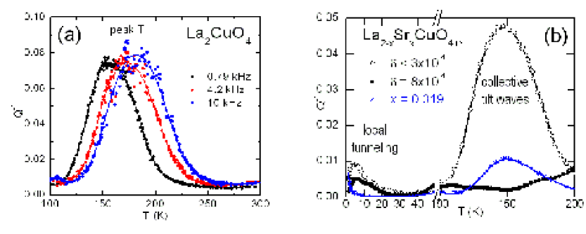
Figure 4-15: (a) peak T attributed to the tilt waves of the octahedra in stoichiometric La₂CuO₄ measured at three frequencies. (b) Blocking effect of $8\times 10^{-4}$ excess O and 0.019 substitutional Sr on peak T and on the relaxation at LHe temperatures.

A possible picture of the excitations involving the planes of CuO₆ octahedra has been provided by Markiewicz [90]. In a model of rigid octahedra free to tilt as in the LTO structure (Fig. 4-1), the tilt of an octahedron propagates all over the plane (Fig. 4-16a), but if the rotation axes pass through the CuO bonds as in the LTT case, the correlations are only in rows of octahedra along directions perpendicular to the tilt axes, since they share the O atoms which are displaced from the CuO plane, while adjacent rows are little correlated, since the share O atoms remaining in the CuO plane (Fig. 4-16b). Markiewicz therefore observed that a system with LTT ground state is reduced to a one-dimensional array of rows of octahedra, where all the octahedra belonging to the same row are tilted according to the same pattern. The resulting equations of motion are non-linear and admit solitonic solutions, which correspond to one-dimensional propagating walls between domains with different tilt patterns [90], as schematically represented in Fig. 4-16c). Although extended X-ray absorption fine structure [85] (EXAFS) and atomic pair distribution function [38] (PDF) measurements of La_2-xSr_xCuO₄ exclude a prevalent LTT local tilt at small $x$, the model by Markiewicz [90] of a LTO structure arising from a LTT ground state (dynamic Jahn-Teller phase) seems to provide a good framework for analyzing the dynamics of the connected octahedra without charge doping.

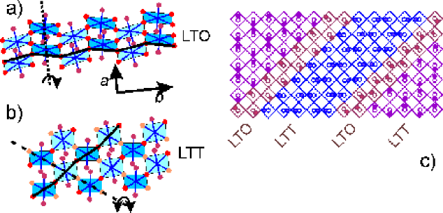
Figure 4-16: Tilt patterns of the LTO (a) and LTT (b) phases; (c) possible representation of tilt waves, where only the apical atoms (filled circles) and their average positions (empty circles) are represented.

Additional evidence that peak T is connected with the oxygen octahedra and more insight on the nature of motion involved came from the collaboration with Rigamonti and Corti, who made Nuclear Quadrupolar Resonance (NQR) experiments on the same samples measured by us [91]. Details on the NQR principles and technique can be found in Refs. [91, 17] and will be omitted here for reasons of space. I will only mention that in those experiments the spins of the ¹³⁹La nuclei can be driven out of equilibrium by radio frequency pulses, and the effective relaxation rate $W_{\text{Q}}$ for reaching equilibrium can be measured. Such a rate is determined in the present case by the fluctuations of electric field gradient (EFG) at the La nuclei, and in particular by the fluctuating displacements of the surrounding apical O atoms. Under such conditions, there is correspondence between $W_{\text{Q}}\left(\omega,T\right)$ and $Q^{-1}\left(\omega,T\right)$, since [17]

$$W_{\text{Q}}\left(\omega,T\right)\propto\int dt\,e^{-i\omega t}\left\langle x\left(t\right)x\left(0\right)\right\rangle=J\left(\omega,T\right)$$ (4.11)

where $J$ is the spectral density of the displacements $x$ of the apical O atoms. On the other hand, as shown in Sec. 2.2, also $Q^{-1}\left(\omega,T\right)\propto J$, since the same displacements, for nearly rigid octahedra, are coupled to the in-plane shear. Therefore, if such displacements produce peak T in the elastic energy loss, they must also produce a peak in $W_{\text{Q}}\left(\omega,T\right).$ This has been indeed observed [91], as shown in Fig. 4-17.

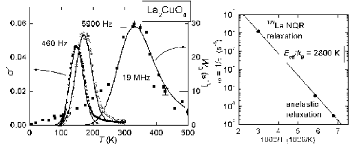
Figure 4-17: Peak T after subtraction of the background measured in the anelastic $Q^{-1}$ and ¹³⁹La NQR relaxation rate. Also shown is the Arrhenius plot $\tau^{-1}$ deduced from the three maxima.

The relaxation rate $\tau^{-1}$, determined from the condition $\omega\tau=1$ at the maxima of the $Q^{-1}\left(T\right)$ and $W_{\text{Q}}\left(T\right)$ curves, is also plotted in logarithmic scale against the reciprocal of temperature. The three points can be closely fitted by a straight line $\tau^{-1}=\tau_{0}^{-1}\exp\left(-E_{\text{eff}}/k_{\text{B}}T\right)$, $\tau_{0}=1.9\times 10^{-12}$ s and $E_{\text{eff}}/k_{\text{B}}=2800~{}$K, clearly indicating that the same process is observed by both techniques. Both sets of curves have been fitted (continuous lines) with $\tau_{0}=$ $1.7\times 10^{-12}~{}$s integrating over a gaussian distribution of $E_{\text{eff}}/k_{\text{B}}$ with mean value $2800~{}$K and width of $\sim 300~{}$K [91].

In order to gain some insight on the nature of the barrier $E_{\text{eff}}$, one should develop the statistical mechanics of the one-dimensional model of correlated tilts of Markiewicz [90], which is a rather difficult task. However, one can apply the one-dimensional models of non-linear lattice dynamics [92], which have been used to describe the correlated dynamics of off-centre atoms in perovskites [93]. In these models the $i$-th atom moves in a double-potential of the form $V=\sum_{i}-ax_{i}^{2}+\,bx_{i}^{4}+\,\overline{c}x_{i}x_{i+1}$, with minima separated by an energy barrier $E=(a^{2}/4b)$ and with a bilinear coupling to the neighbors. The coupling constant $\overline{c}$ takes into account a cluster average over configurations. The resulting equation of motion has solitonic solutions similar to those found for the octahedra in La₂CuO₄,[90] and it has been shown [92, 93] that the spectral density $J\left(\omega\right)$ of the displacements $x$ contains a resonant peak at the frequency of vibration in each minimum, and a central peak due to the jumps to the other minimum with mean hopping frequency $\tau^{-1}=\tau_{0}^{-1}\exp\left(E_{\text{eff}}/T\right)$ with effective barrier $E_{\text{eff}}\approx 1.75E\sqrt{2\overline{c}/a}$, increased with respect to the local barrier $E$ by the interaction between the octahedra, and $\tau_{0}=\frac{d}{v}\sqrt{\overline{c}/a}$, where $v$ is the average velocity of propagation of the soliton-like excitation through the atoms spaced by $d$.

The central peak (see Sec. 2.2) is therefore responsible for the peak in the NQR relaxation rate and in the elastic energy loss; the effective barrier $E_{\text{eff}}/k_{\text{B}}=2800$ K is compatible with the theoretically estimated [42, 48] local barrier of $\sim 500~{}$K (see also Sec. 4.1.2) assuming a mean coupling constant $\overline{c}_{0}\simeq 10a$. The width of the gaussian distribution of $\bar{c}$ is $\sigma=0.18\overline{c}_{0}$ for the NQR and $0.25\overline{c}_{0}$ for the anelastic data and is justified by the distribution in size and shape of the regions where the octahedra clusters build up the cooperative dynamics; such regions are delimited by O${}_{\text{i}}$, which blocks the relaxational dynamics. An asymmetry energy $\Delta E=280~{}$K, 10 times smaller than $E_{\text{eff}}$, has been assumed to reproduce the increase of the intensity of the anelastic peak T, and may also be justified as follows. For nuclear quadrupolar relaxation to occur it is sufficient that a solitonic front passes near a ¹³⁹La nucleus producing a fluctuation of the atomic positions; for anelastic relaxation to occur, instead, it is necessary that a strain fluctuation occurs, and the simple propagation of a tilt wave is not sufficient: referring to Fig. 4-16c, for example, it is necessary that also the size of an LTT region changes with respect to the neighboring LTO region, since LTT and LTO regions have different strain (in other words it must be $\Delta\lambda\neq 0$ in Eq. (2.15)); such a process involves energetically inequivalent states and therefore $\Delta E\neq 0$.

The proposed physical picture is therefore that tilt waves can arise, propagate with a velocity determined by the coupling $\overline{c}$ between rows of octahedra, and disappear within regions free of defects that can block the tilt degrees of freedom (O${}_{\text{i}}$ in the first place, substitutional Sr and twin boundaries). The creation and annihilation of such excitations would result in strain fluctuations and therefore anelastic relaxation. On the other hand, such tilt waves could extend over more than few tens of lattice spacings only in accurately outgassed and defect-free crystals and would have little or no correlation along the $c$ axis, making difficult their observation by diffraction techniques. The lack of correlation among different planes would be the main difference between these tilt solitons and the usual twin boundaries and, to my knowledge, La₂CuO₄ is a unique case exhibiting this type of lattice excitations. The conditions necessary for their existence are: i) the existence of unstable lattice modes describable by a one-dimensional non-linear equation of motion (therefore having solitons as possible solutions); ii) a low density of pinning centers, in order to allow the formation and propagation of such excitations to occur. La₂CuO₄ satisfies both conditions, since it has planar arrays of octahedra with little coupling between different planes, and with the further possibility of decoupling each plane into rows [90]; in addition, the level of defects and impurities can be lowered enough to let these solitonic tilt waves to develop. I tried to observe similar effects in the isostructural La₂NiO_4+δ, but in that case it is impossible to lower the content of O${}_{\text{i}}$ below acceptable levels. Another isostructural material with planes of octahedra close to an instability is Sr₂RuO_4+δ, but it might present problems with excess oxygen [94], and above all the instability is rotational about the $c$ axis [95]. In that case the rotation of an octahedron is strongly coupled to the rotations of all the octahedra in the plane, excluding the possibility of a one-dimensional equation of motion; it is also intuitive that when a rotation of a single octahedron determines the rotations of the neighboring octahedra in both $x$ and $y$ directions, excitations like these cannot arise (see also Fig. 6-4). Indeed, such rotations would be coupled to the $c_{66}$ elastic constant, which however stiffens normally below 220 K [96]. Also in RuSr₂GdCu₂O₈ the octahedra are tilted about the $c$ axis, and in fact its low temperature anelastic spectrum does not show any anomaly of this type [97].

4.10 Tunneling driven local motion of the oxygen octahedra

This section is devoted to peak #4 in Fig. 4-8, also shown in Fig. 4-15b and indicated as ”local tunneling”, and studied in Refs. [79, 98]. For this relaxation process, which I label here as LT, it is possible to make considerations similar to those made in the previous section for peak T. Its intensity, again better appreciated from a modulus defect up to 10% (Fig. 4-18a), is extraordinarily high if one considers that at 10 K only small atomic displacements that driven by tunneling may occur. Therefore, a great fraction of the lattice must participate in the motion, and, again, the unstable tilt modes of the octahedra are the first candidates, but on a local scale (single octahedra or even oxygen atoms).

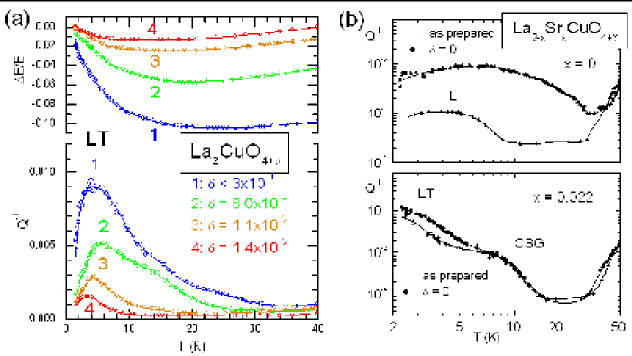
Figure 4-18: Effect of excess O on the relaxation processes LT attributed to O tunneling (a) in a Sr-free sample and (b) in Sr-doped LSCO, where peak LT is accompanied by the relaxation of domain walls in the CSG phase (CSG).

A confirmation from this hypothesis comes from the effect of O${}_{\text{i}}$: with increasing $\delta$ the relaxation amplitude is depressed (Fig. 4-18a), since the tilts of the octahedra surrounding O${}_{\text{i}}$ are fixed to accommodate the interstitial. Still, the effect is much less marked than for the collective motion, as can be appreciated from Fig. 4-15b, where in the curve for $\delta=8\times 10^{-4}$ peak T is completely absent, but peak LT is only halved in intensity. It also appears that the peak shifts to lower temperature with increasing doping, and I will show now that this effect has to be attributed to the holes doped by O${}_{\text{i}}$.

The effect of hole doping is better studied by substitution of La with Sr, which we have seen disturbs the lattice much less than O${}_{\text{i}}$, and reveals extremely interesting effects of lattice-charge coupling, also providing evidence that such a local motion is dominated by atomic tunneling. The introduction of holes above $\sim 0.01$, however, introduces another relaxation process attributed to the motion of the domain walls (hole stripes) in the cluster spin glass (CSG) phase, as discussed in Sec. 4.11.1, which has to be distinguished from peak LT. Figure 4-18b shows the low temperature anelastic spectra of La_2-xSr_xCuO₄ at $x=0$ and $x=0.022$, where the Sr-doped sample presents an additional step around 10 K in correspondence with the freezing into the CSG phase. The different nature between the tunneling process, LT, and the CSG absorption is put in evidence by the fact that excess O depresses peak LT (in the as-prepared state) in both samples, but does not affect the CSG step at all. This fact allows the two processes to be distinguished from each other.

Figure 4-19 shows the $Q^{-1}\left(T\right)$ curves of outgassed LSCO at four doping levels between $0<x<0.028$. What appears from the first three curves at $x=0$, 0.007 and 0.015 is that Sr doping has two extremely marked effects on peak LT: i) a shift to lower temperature, ii) a narrowing and iii) an increase of the intensity. Already at a doping level as low as $x=0.015$ the maximum of peak LT is below our experimental temperature window, and therefore it is impossible to say whether the intensity is still higher than that, already considerable, of the curve for $x=0.007$. For $x=0.028$ even the tail of the relaxation is no more visible. The effect of shift to lower temperature is also observable with doping with O${}_{\text{i}}$ (Fig. 4-18b), but is obscured by the concomitant depression due to blocking.

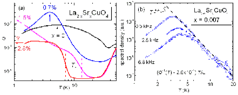
Figure 4-19: Left: elastic energy loss coefficient of slightly doped LSCO at LHe temperature. The arrows indicate peak LT; the steps in correspondence with the vertical bars at $T_{g}\left(x\right)$ are due to the onset of the CSG phase. Right: peak LT for $x=0.007$ measured at three frequencie, after subtraction of a constant backgroung.

With Sr doping the blocking effect is reduced and it appears that doping has a very strong effect on the low temperature relaxation: it increases its intensity and shifts it to lower temperature, which implies an acceleration of the pseudodiffusive dynamics of the octahedra. Unfortunately the relaxation could be followed only up to the very small doping level of $x=0.015$, and it is impossible to extrapolate to the superconducting region of the phase diagram.

The peak for $x=0.007$ is sufficiently well defined to be analyzed, and Fig. 4-19b shows the spectral density $J\left(\omega,T\right)=\frac{T}{\omega}Q^{-1}\left(T\right)$ measured on the three vibration modes in double logarithmic scale, after subtraction of a common constant background. It appears that all the curves collapse together in the high temperature region, as expected from a process that is a superposition of Debye relaxations with some distributions $g\left(\tau\right)$ and $h\left(\Delta\right)$ of relaxation times and strengths. In fact, at high temperature one can discard $\left(\omega\tau\right)^{2}$ in the denominator of Eq. (2.34) and set $J\left(\omega,T\right)=\frac{T}{\omega}Q^{-1}\left(T\right)\simeq T\int d\tau\,g\left(\tau\right)\int d\Delta\,h\left(\Delta\right)\,\tau$ which is independent of $\omega$. The $J\left(\omega,T\right)$ obtained for $x=0$ does not satisfy the same condition, because it is described by a broad distribution of $\tau\left(T\right)$ which vary with temperature at a slower rate than in the case $x>0$, so that the condition $\omega\tau\ll 1$ is not satisfied in the high temperature side of the peak for all the elementary relaxations. Therefore, from the temperature position and shape of peak LT we deduce that doping changes the mean relaxation rate $\tau^{-1}$ from a slowly varying function of temperature in the undoped case to a function which increases faster with temperature. The high temperature side of $J\left(\omega,T\right)$ indicates that, for $x=0.007$, the rate $\tau^{-1}$ increases faster than $T^{4}$ above 6 K.

The above analysis demonstrates that peak LT is due to atomic displacements changing at an average rate $\tau^{-1}$, and both the low temperature of the maximum and the fact that $\tau^{-1}\propto T^{n}$ indicate that the rate is not due to overbarrier hopping with the Arrhenius law, but is determined by quantum effects. In the standard tunneling model, the changes of average atomic positions with rate $\tau^{-1}$ are associated with transitions of the tunnel system (TS) between its eigenstates [99]. The eigenstates arise from the overlap of the atomic wave functions (of a single oxygen or possibly of a whole octahedron in our case) over two or more minima of the multiwell potential, like that of Fig. 4-4b; the transitions between the eigenstates are promoted by the interaction between the TS and the various excitations of the solid, generally consisting of emission and absorption of phonons and scattering of the conduction electrons [99]. An important difference between the relaxation process LT and those due to TS in glasses is that the latter are characterized by an extremely broad distribution of parameters, mainly the tunneling energy $t$ and the asymmetry between the minima of the double-well potential; instead, in La_2-xSr_xCuO₄ the geometry of the tunnel systems is much better defined, being some particularly unstable configurations of the octahedra. As a consequence, the TLS relaxation in glasses produces a plateau in the acoustic absorption and a linear term in the specific heat as a function of temperature, whereas in La_2-xSr_xCuO₄ we observe a well defined peak in the absorption, and no linear contribution to the specific heat has been reported.

4.10.1 Interaction between the tilts of the octahedra and the hole excitations

I argue now that the marked acceleration of the local fluctuations with doping (narrowing and shift to lower temperature of peak LT) is the manifestation of a direct coupling between the tilts of the octahedra and the holes, similarly to the TS in metals, whose dynamics is dominated by the interaction with the conduction electrons [99]. The transition rate of a TS is generally of the form

$$\tau^{-1}\left(T\right)\propto t^{2}\left[f_{\text{ph}}\left(T\right)+f_{\text{el}}\left(T\right)\right]\,,$$ (4.12)

where $t$ is the tunneling matrix element and $f_{\text{ph}}\left(T\right)$ and $f_{\text{el}}\left(T\right)$ contain the interaction between the TS and the phonons and electrons, whose excitation spectra depend on temperature and hole density. As shown in Sec. 4.1.1 and Fig. 4-3b, doping reduces the tilt instability and tilt angle of the octahedra, and hence makes the minima of the multiwell potential closer to each other and reduces the potential barriers between them, resulting in a larger $t$ [80]. Such changes are however gradual, and a doping as low as $x=0.007$ can hardly account for the drastic rise of $\tau^{-1}$ only through an increase of $t$. The greater contribution has to be attributed to the increased interaction with the doped holes, corresponding to the term $f_{\text{el}}\left(T\right),$which is null in the perfectly undoped material, but immediately becomes $\gg f_{\text{ph}}$. Models for the interaction between tunneling systems and electrons have been developed and successfully adopted, but the electronic excitation spectrum of the cuprate superconductors is certainly different from that of metals, and new models for the interaction between octahedra and holes are needed. In fact, the asymptotic behavior of $J\left(\omega,T\right)$ at high and low temperature for $x=0.007$ indicate that $f_{\text{el}}\left(T\right)\sim T^{n}$ with $n\sim 3-5$, completely different from TS in standard metals, where $f_{\text{el}}\left(T\right)$ is less than linear [99].

Unfortunately, with the present experiments it has been possible to follow peak LT only up to $x=0.015$, but it cannot be excluded that the pseudo-diffusive lattice modes giving rise to peak LT modify the electron-phonon coupling at higher doping. In fact, the characteristic frequencies of these modes are far too low for having any influence on the electron dynamics for $x\leq 0.02$, but increase dramatically with doping. In terms of the multiwell lattice potential, it is possible that at higher doping the barriers between the minima become small enough to give rise to an enhancement of the electron-phonon coupling predicted by some models with anharmonic potentials [100].

4.10.2 Static and dynamic tilt disorder

The observation of an increased intensity of peak LT at $x>0$ with respect to $x=0$ (Fig. 4-19a) provides an explanation for the apparent discrepancy between the tilt disorder observed by anelastic experiments on La₂CuO_4+δ on one side and EXAFS [85] and atomic PDF [38] measurements on La_2-xSr_xCuO₄ on the other side. The anelastic spectra of Fig. 4-18 indicates a dynamic tilt disorder increasing with reducing $\delta$ (and therefore doping), while the latter techniques see the opposite effect of an increasing tilt disorder with increasing doping through $x$. Actually, the EXAFS spectra and atomic PDF are sensitive to both static and dynamic disorder; at $x=0$ the instantaneous fraction of octahedra swept by the tilt waves is relatively small; according to a crude estimate [91] a few percents of octahedra instantaneously involved in the tilt waves account for the intensity of NQR relaxation (peak T) and their effect on the PDF or EXAFS spectra would be undetectable. At higher $x$, the instantaneous tilt disorder will increase due to both the disorder in the La/Sr sublattice and the lattice fluctuations. Instead, the anelastic spectroscopy is sensitive only to the dynamic disorder with characteristic frequency comparable to the measurement frequency; the introduction of interstitial O certainly increases the static tilt disorder but also inhibits the dynamic one, resulting in the depression of peaks LT and T observed in Figs. 4-18 and 4-11. By introducing substitutional Sr, which disturbs the lattice much less than interstitial O, it is possible to observe that doping actually increases the fraction of fluctuating octahedra, and not only the static disorder.

4.11 Charge and spin inhomogeneities on nanometer scale

4.11.1 The cluster spin glass phase: fluctuations of the hole stripes between the pinning points

The low-temperature anelastic spectrum of LSCO presents a step-like increase of the absorption below a doping-dependent temperature $T_{g}\left(x\right)$, as already noted in Figs. 4-18b and 4-19a. Figure 4-20 clearly shows that the temperature at which the increase of $Q^{-1}$ occurs is in close agreement with the temperature $T_{g}\left(x\right)$ for freezing into the cluster-spin glass (CSG) state (Sec. 4.3 and Fig. 4-3). As also discussed in Refs. [101, 62], $T_{g}$ is not easy to be determined, and is often identified with the temperature $T_{f}\left(\omega\right)$ at which the rate of the spin fluctuations falls below the frequency $\omega$ probed by the experiment, $>10^{11}$ s^-1 for neutron scattering [58], $10^{8}-10^{9}$ s^-1 for NMR/NQR [102], $10^{6}$ s^-1 for muon spin relaxation [54] $10^{3}-10^{5}$ s^-1 for anelastic spectroscopy and $<0.1$ s^-1 for magnetization measurements [101]. A system with glassy dynamics is generally describable with a broad distribution of relaxation times $\tau$, and the maximum relaxation time $\tau_{\text{M}}$ of such a distribution diverges at $T_{g}$, often following the Vogel-Fulcher law $\tau_{\text{M}}=\tau_{0}\exp\left[\frac{E}{k_{\text{B}}\left(T-T_{g}\right)}\right]$, resulting in a maximum of the dynamic susceptibilities at $\omega\tau_{\text{M}}\simeq 1$. By adopting the above criterion, one measures the freezing temperatures $T_{f}\left(\omega\right)$ such that $\omega^{-1}\sim\tau_{0}\exp\left[\frac{E}{k_{\text{B}}\left(T_{f}-T_{g}\right)}\right]$, and the lower is $\omega$ the closer $T_{f}$ approximates $T_{g}$. For the case of freezing into the CSG state in LSCO, it seems that $\tau_{\text{M}}$ diverges fast enough that $T_{f}$ measured by magnetization is a good estimate of $T_{g}$ and can be well approximated by the expression [74]

$$T_{g}\left(x\right)\simeq\left(0.2~{}\text{K}\right)/x\,.$$ (4.13)

The vertical bars in Fig. 4-20 are obtained from this expression of $T_{g}\left(x\right)$ and have an excellent correlation with the rise of $Q^{-1}\left(T\right)$ [103, 61, 62], clearly indicating that the acoustic absorption is correlated to the CSG state. A strong indication that the absorption step in the CSG state is of magnetic origin within the CuO₂ planes is its complete insensitiveness to interstitial O, as shown in Fig. 4-18b, whereas the rest of the anelastic spectrum, involving tilts of the octahedra, is drastically affected by the presence of even minute amounts of O${}_{\text{i}}$.

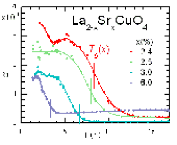
Figure 4-20: Step in the $Q^{-1}$ below the temperature $T_{g}$ for freezing into the cluster spin glass state at different dopings.

Regarding the mechanism producing dissipation, it might be similar to the well known stress-induced movement of domain walls (DW) in ferromagnetic materials [8, 9]. In this case, the spin order is antiferromagnetic (AF), and the anisotropic strain might be correlated with the easy axis $\mathbf{\hat{m}}$ for the staggered magnetization [103]. The elastic energy of domains with different orientations of $\mathbf{\hat{m}}$ would be differently affected by a shear stress, and the domains with lower energy would grow at the expenses of those with higher energy. According to the prevalent interpretation presented in Sec. 4.4, the walls between the AF clusters should be the charge stripes where the holes are segregated, and therefore the acoustic absorption below $T_{g}$ would be due to the fluctuations of the hole stripes. According to this view, the rise of $Q^{-1}\left(T\right)$ would be determined by the freezing of the spins into AF domains with some disorder in the directions of the staggered magnetization $\mathbf{\hat{m}}$. According to neutron diffraction and magnetic susceptibility, in La₂CuO₄ or slightly doped La_2-xSr_xCuO₄ ($x<0.03$) the direction of $\mathbf{\hat{m}}$ is parallel to the $b$ axis [52], but we suppose that some distortion of the spin order must be present, like e.g. in Gooding’s model [53], otherwise the anisotropic strain would be parallel to $b$ in all domains and there would be no anelastic relaxation. Note that the fact that the hole stripes must have fluctuations and topological defects at all temperatures is predicted by several authors [104, 105, 106], but what is needed here is disorder in the average direction of $\mathbf{\hat{m}}$ from domain to domain. Within this picture, the diffraction experiments see the ordered fraction of stripes, with regular spacing and separating antiphase AF domains, while anelastic relaxation is due to the disordered fraction of the spin structure. The relaxation of DW pinned by impurities, the Sr dopants in our case, is generally characterized by a broad distribution of relaxation times, and this would explain why a plateau rather than a peak is observed. The $Q^{-1}\left(T\right)$ step at $T_{g}$ would than be analogous to the $Q^{-1}\left(T\right)$ step occurring at $T_{t}$ in correspondence with the structural HTT/LTO transformation with consequent formation and motion of twin walls (see the step #1 followed by the broad peak #2 in Fig. 4-8).

A possible alternative or concomitant mechanism of relaxation within the CSG phase is the motion of kinks on the otherwise straight stripes, in analogy with the motion of kinks in dislocations [9]. The dynamics of such kinks in the hole stripes has been theoretically analyzed [60], also in the presence of pinning, and seems to correspond to another anelastic relaxation process attributed to collective stripe depinning, as described in Sec. 4.11.3.

The above results indicate that the anelastic relaxation below $T_{g}$ is due to the stripe fluctuations, when they act as walls between frozen AF domains. On the other hand, it has been established that the stripes can be locked by the LTT structure, when they are parallel to the LTT modulation (for $x>0.055$ [59, 70]) and commensurate with it ($x=\frac{1}{8}$ [56, 57]). The time scale of the neutron scattering experiments that established this phenomenology is extremely short, and what appears static in those experiments may be fast for low frequency anelastic spectroscopy; nonetheless, in case of real locking of the stripes by the LTT structure, the absorption step at the CSG transition should be depressed of the fraction of stripes that become static. For this reason, we extended the anelastic measurements to La_2-xBa_xCuO₄ (LBCO) [61], that has a greater tendency to form the LTT phase (see Fig. 4-5).

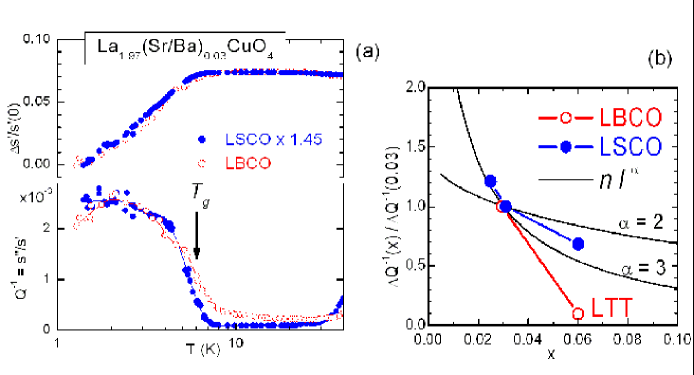
Figure 4-21: (a) Compliance of LBCO and LSCO (rescaled to overlap with that of LBCO) with 3% Sr. (b) Doping dependence of the intensity of the $Q^{-1}$ step at $T_{g}$ for LSCO and LBCO, compared with the relaxation amplitude expected from dislocations ($\alpha=3$) or ferromagnetic domain walls ($\alpha=2$).

Figure 4-21a shows both the absorption and real parts of the compliance of LSCO and LBCO at $x=0.03$. The data of LSCO practically overlap with those of LBCO if multiplied by 1.45, and the onset of the decrease of the compliance coincides with $T_{g}$, indicating that it is determined by the same mechanism producing the absorption, i.e. the freezing of the stripe fluctuations. The factor $\sim 1.5$ can be ascribed to a greater magnetoelastic coupling in the Ba compound, possibly resulting from the slightly different atomic sizes and distances.

Figure 4-21b presents the amplitude of the $Q^{-1}$ step at $T_{g}$ for LSCO at $x=0.025$, 0.03 and 0.06, and of LBCO at $x=$ 0.03 and 0.06 normalized to the value assumed at $x=0.03$. These data are compared with the relaxation strengths expected from dislocations, $\Delta_{\text{d}}\left(x\right)$, and from ferromagnetic DW, $\Delta_{\text{DM}}\left(x\right)$, strongly pinned by a concentration $x$ of defects in a bidimensional geometry. In both cases a power law $\Delta\propto n\left(x\right)l^{\alpha}\left(x\right)$ is expected, with $l$ the mean length between pinning points, $n$ the line density and with $\alpha=3$, in the case of dislocations [8] or $\alpha=2$ in the case of FM DW [107]. The $\Delta\left(x\right)$ curves have been calculated assuming that the stripes are fixed at the pinning points [61], obtaining $\Delta\propto 2x\left(\frac{1}{\sqrt{x}}-1\right)^{\alpha}$, as explained in Appendix C. In this manner, the experimental data of LSCO are reasonably well reproduced with $\alpha\lesssim 3$, intermediate between the dislocation and DW cases. It should be remarked that the condition of strong pinning, namely that the walls are really pinned at the dopants and can move only between them [107], is probably not verified. In fact, as discussed in Sec. 4.11.3, Morais Smith et al. [60] estimate that the stripes in LSCO are in the weak pinning regime, where the stripe may accommodate into the pinning potential over a collective length $L_{c}$ enclosing several pinning centers. Nonetheless, the dependence of $\Delta Q^{-1}$ for LSCO on $x$ is intermediate between that typical of ferromagnetic DW and that of dislocations, and this appears as an indication that indeed the relaxation process below $T_{g}$ and therefore the stripe fluctuations in the CSG phase can be assimilated to the motion of line defects pinned by the Sr dopants.

Comparing now the data on LSCO with those on LBCO in Fig. 4-21b, it turns out that when La is substituted with 6% Ba instead of 6% Sr, then $\Delta Q^{-1}$ is $\sim 7$ times smaller than expected. This depression has to be attributed to the transformation into the LTT structure below $T_{d}\simeq 40$ K, as indicated by the upward inflection in the Young’s modulus observed only for La_2.94Sr_0.06CuO₄ (Fig. 4-10), and is a clear indication of pinning of the DW motion within the LTT phase, which causes a modulation of the potential felt by the holes, as explained in Sec. 4.1.2. As explained in Sec. 4.7.2, there are indications of the formation of LTT domains also in LSCO, but only in LBCO and LSCO co-doped with Nd a stable LTT phase with long range order sets in, which can provide a pinning potential for the stripes (see Sec. 4.1.2). Only the stripes parallel or nearly parallel to this modulation should be clamped, and therefore from the reduction factor $\sim 7$ we deduce that about 87% of the DW are parallel to the direction of the Cu-O bonds in the LTT phase (or even more if the transition to the LTT structure is incomplete); this stripe orientation is in agreement with the direction of the magnetic modulation observed by neutron scattering for $x\geq 0.055$ [59].

The pinning of the DW of the CSG phase within the LTT structure is well documented for $x\simeq\frac{1}{8}$, when the stripe spacing is commensurate with the lattice spacing [56, 57]. Figure 4-21 demonstrates that almost complete pinning of the stripes can occur also at $x=0.06$, far from the condition of commensurability with the lattice; in addition, the anelastic spectroscopy provides evidence of pinning over a time scale $\tau>$ $\omega^{-1}\sim 10^{-3}$ s, much longer than the time scale of neutron diffraction, demonstrating that the pinned stripes are really static.

4.11.2 Electronic phase separation at $x<x_{c}$

The study of the low-temperature anelastic spectrum of LSCO has been concentrated around the critical doping $x_{c}\simeq 0.02$ above which no more long ranged AF order exists (Fig. 4-3), on samples with nominal doping $x=0.015$, 0.016, 0.018, 0.024, 0.03. The prevalent view is that for $x<x_{c}$ a spin glass (SG) state still occurs, but different from the CSG one both in the nature (long range AF order with uncorrelated spin distortions near the dopants instead of AF clusters) and doping dependence of the freezing temperature $T_{f}$ ($T_{f}\propto x$ instead of $T_{g}\propto 1/x$). This differences should appear also in the anelastic spectra, since in this picture there are no walls in the SG state; therefore, below $x_{c}$ there should be no step-like rise of the acoustic absorption at $T_{f}$, or possibly one expects a sharp peak corresponding to those appearing in the NQR and $\mu$SR relaxation rates, in correspondence with the crossover for spin fluctuations becoming slower than the experimental frequency [17] (the condition $\omega\tau\simeq 1$). On the contrary, the anelastic spectra at $x<x_{c}$ present the same $Q^{-1}\left(T\right)$ step as for $x\simeq 0.02$, at nearly the same temperature but with smaller amplitude [103, 63]. The temperatures of the $Q^{-1}\left(T\right)$ steps found for both $x>x_{c}$ and $x<x_{c}$ are plotted as open circles in the region of low-$T$ and low-$x$ of the phase diagram of LSCO in Fig. 4-22, where also the canonical $T_{f}\left(x\right)$ and $T_{g}\left(x\right)$ lines are indicated, and there is no hint of a crossover from $T_{f}\left(x\right)$ to $T_{g}\left(x\right)$.

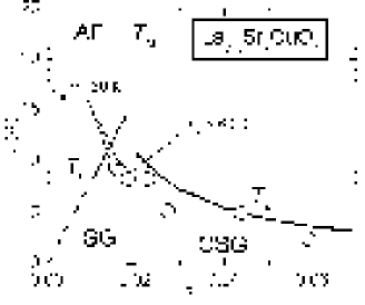
Figure 4-22: Low-$T$ and low-$x$ region of the phase diagram of LSCO. The open circles are $T_{g}$ deduced from the step in the $Q^{-1}\left(T\right)$ curves.

In view of the difficulties in preparing samples with $x$ determined to better than 0.1% and considering the possibility of inhomogeneities in the Sr distribution, we carried out a rather accurate characterization of our samples. The Sr content $x$ was checked from the temperature $T_{t}\left(x\right)$ of the HTT/LTO transformation and the homogeneity was checked from the width of the transformation appearing in the $Q^{-1}\left(T\right)$ and $E\left(T\right)$ curves, as explained in Sec. 4.7.1. The deviations of the resulting $x$ from the nominal value were not important, as shown Fig. 4-9b, and no inhomogeneity could be detected, to justify regions with $x>0.02$ in samples with $x\leq 0.018$. The magnetic state of the samples was characterized by means of NQR and SQUID measurements performed by M. Corti and A. Rigamonti in Pavia: $T_{\text{N}}$ of the samples with $x=$ $0.015$ and 0.016 was $\sim 150$ K, while for $x=$ $0.018$ it was only possible to obtain an upper limit $T_{\text{N}}<60$ K, due to the overlap with the intense maximum in the ¹³⁹La relaxation rate usually attributed to spin freezing.

It can be concluded that the similarity of the anelastic spectra for $x<0.02$ with those for $x>0.02$ is a real effect and not due to poor samples. The anelastic data are then in perfect agreement with the neutron scattering experiment by Matsuda et al.[55] on the magnetic correlations in La_2-xSr_xCuO₄ for $x<x_{c}$, where it is found that also at $x<x_{c}$ the 3D AF ordered phase coexists below $\sim 30$ K with domains of ”diagonal” stripe phase (with the hole stripes at $45^{\text{o}}$ with respect to the Cu-O bonds). According to these authors, the hole localization starting around 150 K involves an electronic phase separation into regions with $x_{1}\sim 0$ and $x_{2}\sim 0.02$, and variations in doping affect only the volume fractions of the two phases. The $Q^{-1}$ step in samples with $x<0.02$ [103, 63] is therefore due to the fraction with $x_{2}\sim 0.02$, so explaining the fact that the onset of the absorption occurs at the same temperature appropriate for the local doping $x=x_{2}$, while the decrease of the absorption amplitude reflects the decrease in the phase with $x=x_{2}$.

4.11.3 Thermally activated depinning of the charge stripes

The elastic energy loss rise in correspondence with the freezing into the CSG phase discussed in the previous section, although connected with the stripe fluctuation, exists only below $T_{g}$, and for this reason is attributed to magnetoelastic coupling with the AF domains rather than to the stripes themselves. The charge stripes, however, do exist also at higher temperature, e.g. in LSCO substituted with Nd and 12% Sr the superlattice peaks of charge order appear below 70 K [56], and various types of phase diagrams with charge stripes at temperature well above that of the spin glass state are extensively discussed [5, 2]. Carrying on the analogy between the charge stripes and other linear defects, like dislocations or domain walls, we tried to identify a possible anelastic signature of the stripes that overcome the pinning potential by thermal activation, and found that a relaxation process with maximum at $\sim 80$ K for $\sim 1$ kHz, here labeled peak S, has all the expected characteristics [65]; in Ref. [65] it is also discussed why alternative explanations should be very unlikely. The peak is evidenced with a red arrow in Fig. 4-23, where the evolution of the anelastic spectrum of La_2-xSr_xCuO₄ from $x=0.018$ to $x=0.20$ is shown. The peak well visible up to $x=0.045$ is peak T discussed in Sec. 4.9 and attributed to the solitonic tilt waves of the octahedra; it is progressively suppressed by the disorder introduced by Sr.

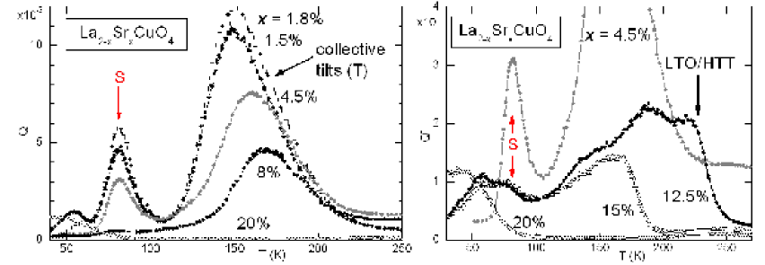
Figure 4-23: Anelastic spectra of LSCO between 50 and 250 K from the underdoped to the overdoped state, measured at $\sim 1$ kHz. The red arrow indicates the peak attributed to the stripe depinning.

For $x\geq 0.125$ the temperature $T_{t}$ of the HTT/LTO transformation becomes lower than 250 K and is easily identifiable as a sharp rise of $Q^{-1}\left(T\right)$ and softening of the Young’s modulus (the latter not shown in Fig. 4-23). Peak S has an intensity with non-monotonic dependence on $x$ and is visible up to $x\leq 0.15$; in the overdoped state, $x=0.20$, there is no trace of the peak, and the only feature of the anelastic spectrum is the HTT/LTO transformation at 70 K. The $Q_{\text{max}}^{-1}\left(x\right)$ data for peak S are reported in the lower part Fig. 4-24b, and it is apparent that the intensity of peak S has exactly the doping dependence expected from a polaronic relaxation due to the hole stripes: i) it vanishes at $x\rightarrow 0$, where there are no holes and therefore no stripes; ii) it vanishes in the overdoped region, $x>0.15$, where the holes are uniformly distributed as in a normal metallic state; iii) it presents an abrupt drop (note the logarithmic scale of Fig. 4-24) between at $x=0.045$ and 0.08, in correspondence with the change of the stripe order from parallel to diagonal with respect to the LTO lattice modulation [59, 70]; iv) it has a local maximum around $x\sim\frac{1}{8}$, where the commensurability between stripe spacing and lattice enhances the stripe-lattice coupling, and the sharp minimum exactly at $x=\frac{1}{8}$ is most likely due to the fact that the locking between LTT lattice fluctuations and stripes is so strong that the fluctuations are depressed. The agreement between the $Q_{\text{max}}^{-1}\left(x\right)$ data and what is expected from a relaxation process due to fluctuations of pinned hole stripes is certainly remarkable, but there is more.

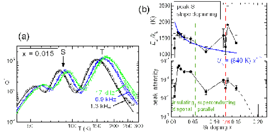
Figure 4-24: (a) Example of fit of the anelastic spectrum of LSCO with $x=0.015$, in order to deduce the activation energy and intensity of the peak attributed to stripe depinning. (b) Doping dependence of the intensity and activation energy of the peak at 80 K (for $\sim 1$ kHz) attributed to the stripe depinning. The blue line is the predicted collective pinning barrier, according to [60].

Figure 4-24a shows the anelastic spectrum for $x=0.015$ from 40 to 300 K measured at three vibration frequencies, which allows peak S together with the neighboring peaks to be reliably fitted, in order to extract the various parameters of the relaxation S and particularly its activation energy, that can be identified with the effective pinning barrier $E_{p}$ (the origin of the peak around 60 K is not yet identified). The continuous curves are a simultaneous fit at all frequencies with Eq. (2.48) for all three peaks. Peak S is rather broad and symmetric, with $\alpha=\beta=0.7$, $\tau_{0}=7\times 10^{-14}$ s and $E_{p}/k_{\text{B}}=1690$ K. Fits like this can be done up to $x=0.045$, while for higher doping there is a larger error in extracting the parameters of peak S, since it is smaller and masked by the other processes. Nevertheless, the doping dependence of $\tau_{0}$ and $E_{p}/k_{\text{B}}$ parameters could be followed over the complete doping range. The dependence of $E_{p}$ on $x$ is particularly interesting, since it closely reflects that of $\log Q_{\text{max}}^{-1}$, as demonstrated in Fig. 4-24. Also the pre-exponential factor $\tau_{0}$ has a general decreasing trend with increasing doping, passing from $1.4\times 10^{-13}$ s to $10^{-10}$ s between $x=0.015$ and $x=0.08$; for this reason the temperature of the peak measured around 1 kHz remains close to 80 K, but it is understood that the peak temperature depends on frequency. Values of $\tau_{0}$ as low as $10^{-10}$ s are certainly too long for a polaronic relaxation, but may be understood in terms of an extended defect like the stripe, with a strong lattice contribution, as argued in what follows.

Before discussing the analogies between the doping dependences of relaxation strength and activation energy, the present results are compared with the predictions of the model of Morais Smith et al. for the dynamics of the pinned stripes [60]. From the balance between the electrostatic interaction $\varepsilon_{c}$ of the hole stripe with the Sr²⁺ dopants, which tends to pin the stripe into a curved configuration, and the elastic energy $\varepsilon_{l}$ for bending the stripe, which tends to keep it straight, both the collective length $L_{c}$ for the stripe reconformations and the pinning barrier $E_{p}$ for such reconformations to occur are estimated. It turns out that

$$L_{c}=ax^{-5/6}\left(\varepsilon_{l}/\varepsilon_{c}\right)^{2/3}$$ (4.14)

where $\varepsilon_{c}=e^{2}/\left(\varepsilon_{0}a\right)\sim 0.1$ eV is the Coulomb energy scale with an isotropic dielectric constant $\varepsilon_{0}\simeq 30\,$and $a\$the lattice parameter, while $\varepsilon_{l}=J\simeq 0.1$ eV is the elastic energy of the stripe determined by the AF exchange constant $J$. Setting $\varepsilon_{l}=J$ tacitly assumes that the hole stripe fluctuates in a static AF background of spins; this is appropriate when the spin fluctuations of the Cu²⁺ atoms are frozen below the characteristic stripe fluctuation frequency under study, as in the CSG state, but certainly not at 80 K for $x>x_{c}$. I suppose that the spin fluctuations would lower the elastic energy $\varepsilon_{l}$ of the stripe, and therefore also $L_{c}$, possibly making a crossover to the strong pinning regime with $L_{c}<l\simeq a/\sqrt{x}$ , where $l$ is the mean distance between pinning centers. Otherwise, with the above estimate of $\varepsilon_{l}\simeq\varepsilon_{c}$ the collective pinning length $L_{c}\simeq ax^{-5/6}\$is always larger than $l$, resulting in the weak pinning regime. The collective pinning energy is estimated as [60]

$$E_{p}=\left(\varepsilon_{l}\varepsilon_{c}^{2}\right)^{1/3}x^{-1/6}\sim\left(1300~{}\text{K}\right)\,\,x^{-1/6}\,.$$ (4.15)

In view of the rough nature of the estimate, especially of $\varepsilon_{c}$, it is reasonable to expect that the $x^{-1/6}$ dependence of Eq. (4.15) can be adopted, but with the constant factor as an adjusting parameter. The blue line in Fig. 4-24 is a fit of $E_{p}\left(x\right)$ of peak S, excluding the $x\sim\frac{1}{8}$ region, with Eq. (4.15), and the constant is found to be $\left(\varepsilon_{l}\varepsilon_{c}^{2}\right)^{1/3}/k_{\text{B}}=840$ K. It can be concluded that the agreement between the general trend of $E_{p}\left(x\right)$ and the predictions for the collective pinning energy barrier of stripes pinned by the Sr dopants of Ref. [60] is surprisingly good, and provides further support to the interpretation of peak S in terms of stripe depinning. It should be noted, however, that the treatment of Ref. [60] does not include the interaction with the lattice, which is at least as important as the electrostatic in interaction with the dopants, as argued in the following Section.

4.11.4 Hole-lattice coupling and octahedral tilts

Regarding the mechanism producing peak S, it would be tempting to simply identify the hole stripe with a dislocation or domain wall, and apply the models of anelastic relaxation from these linear defects, as proposed for the relaxation in the CSG state in Sec. 4.11.1. The problem with peak S is that at 80 K the hole stripes do not separate domains with different orientations of the anisotropic strain, as is the CSG state, since at this temperature the spin fluctuate very fast [17]. Therefore, it is not possible to associate an anelastic strain $\varepsilon^{\text{an}}$ proportional to the area swept by the stripe (the continuum equivalent of the elastic dipole of a point defect), as in the above models. Instead, different strain contributions $\varepsilon^{\text{an}}$ should be associated with the different configurations that the stripe may assume by thermal activation over the pinning barrier, e.g. straight or curved or kinked stripe segment. It is likely that $\varepsilon^{\text{an}}$, like the distortion coupled to the presence of holes [67], is mainly connected with the in-plane shear also associated with the tilts of the octahedra. Then, it is reasonable to assume that $\varepsilon^{\text{an}}$ is an increasing function of the local degree of tilting of the octahedra. This would partly contribute to the general reduction of the relaxation strength with increasing doping, because both the in-plane shear strain and tilt angles $\theta$ of the octahedra are decreasing functions of doping (see Fig. 4-3).

It has already pointed out how the sharp variations of $Q_{\text{max}}^{-1}$ with doping correspond to a variation in the degree of coupling between lattice and stripe; it has to be explained why also the activation energy $E_{p}$ presents similar features. An explanation can be found by observing that the octahedral tilts (the most unstable lattice modes) are responsible for the stripe-strain interaction, and therefore determine the relaxation strength, but also cause stripe pinning from the lattice, as demonstrated by the well known locking between LTT tilt pattern and stripes. Therefore, large tilt amplitudes are associated with both large relaxation strength and strong pinning from the lattice; in other words, anomalies in the tilt-stripe coupling result in anomalies in both $Q_{\text{max}}^{-1}$ and $E_{p}$.

4.11.5 The picture of the slow stripe fluctuations after anelastic spectroscopy

The two anelastic relaxation processes we attribute to the stripe motion are again shown in Fig. 4-25a in a sample with $x=0.03$. In a first instance [103, 61, 65] we assumed a strong pinning regime, where the CSG absorption below $T_{g}$ is due to the motion between pinning points and the 80 K relaxation as the thermally activated depinning process. According to the analysis of Morais Smith et al. [60] the weak or collective pinning regime would be verified also at very low doping, meaning that there is no clear distinction between motion of stripe segments that are between or at the Sr dopants; rather, there is a collective length $L_{c}\left(x\right)$ characteristic for the stripe displacements that minimize the free energy, as mentioned in Sec. 4.11.1 and 4.11.3. If this type of motion produces peak S around 80 K, its contribution becomes totally negligible at $T_{g}<15$ K.

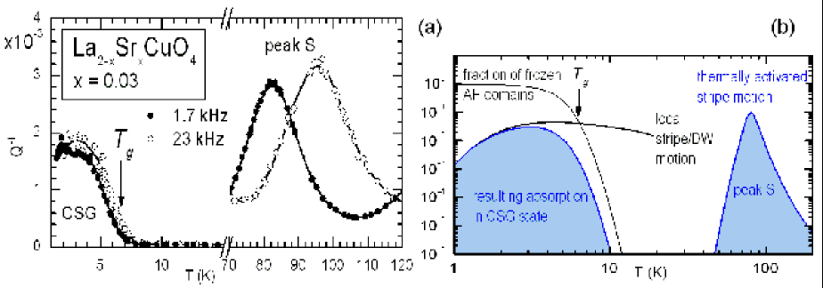
Figure 4-25: (a) Features of the anelastic spectrum of La_1.97Sr_0.03CuO₄ associated with the dynamics of the charge stripes: freezing below $T_{g}$ and thermally activated depinning above 80 K. (b) Sketch of how the absorption below $T_{g}$ might be decomposed into the contribution from DW fast local motion multiplied by the fraction of domains that are frozen.

This is schematically illustrated in Fig. 4-25b with double logarithmic scale, where the extrapolation of peak S is clearly negligible at $T_{g}$. The relaxation appearing below $T_{g}$ must therefore originate from a much faster and probably more local type of stripe motion, indicated as a (totally hypothetical) broad maximum. The fact that the elastic energy loss is seen to grow only below $T_{g}$ indicates that, while the dynamics may be associated to the stripes, the mechanism producing anelasticity involves the frozen AF domains, as discussed in Sec. 4.11.1. This is represented in Fig. 4-25b with the fraction of domains between stripes having a characteristic fluctuation frequency $\tau^{-1}$ frozen below the measurement frequency $\omega$; the resulting $Q^{-1}\left(T\right)$ curve is the product of this fraction with the broad absorption that would be hypothetically measured if the AF spins where already frozen at higher temperature, allowing the mechanism of the stress induced domain wall motion to be operative. The fact that this absorption is broad is indicated by the shape of $Q^{-1}\left(T\right)$ below $T_{g}$.

The mechanism governing the dynamics of the domain wall or stripe motion at these temperatures is necessarily different from the thermally activated overbarrier motion of peak S, and must be totally quantum mechanical. To my knowledge there are no theoretical treatments of this problem; the stripe relaxation time in the quantum limit $\tau\sim 10^{-14}$ s estimated in Ref. [60], based on ohmic dissipation [$f_{\text{el}}\propto T$ in Eq. (4.12)], is far too short for explaining the anelastic relaxation below $T_{g}$ at our frequencies; in fact, the Debye factor $\omega\tau/[1+\left(\omega\tau\right)^{2}]$ would cut the absorption amplitude by a factor of $10^{-10}$, making it unobservable. On the contrary, the broad shape of the $Q^{-1}\left(T\right)$ curve below $T_{g}$ indicates that a consistent weight of the distribution function of the relaxation frequencies is in the kHz range.

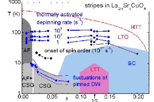
Figure 4-26: Phase diagram of LSCO with the dynamic ranges of the stripe motions deduced from the anelastic experiments.

Figure 4-26 is the phase diagram of LSCO (see Fig. 4-3) with the dynamic ranges of the stripe motions deduced from the anelastic experiments. The depinning rate curves have been calculated from the relaxation time $\tau\left(T\right)\$deduced from peak S; they correspond to the mean relaxation rate for the stripes to overcome the pinning potential from the Sr²⁺ dopants, presumably in the weak pinning regime. As explained in the previous Sections, the relaxation rate reflects the abrupt changes of the effective pinning barrier in correspondence with changes in the stripe-lattice coupling, like the change of the stripe orientation at $x=0.055$ or the possible insurgence of LTT fluctuations near $x=\frac{1}{8}$. The black symbols are the temperatures for the onset of the incommensurate spin order, deduced from the superlattice peaks in magnetic neutron scattering; for $x<0.1$ these temperatures correspond to $T_{g}\left(x,\omega\sim 10^{12}~{}\text{s}^{-1}\right)$, namely the onset of the CSG phase on the neutron scattering time scale [58]. The CSG phase on the (quasi)static time scale from magnetic susceptibility measurements is the gray region. The points labeled ”fluctuations of pinned DW” and the two accompanying upper and lower lines indicate the rise of the acoustic absorption (10%, inflection, 90% of the step) in the CSG phase. The absorption is due to the stress-induced motion of the AF clusters separated by the hole stripes, and in these temperature region there is a substantial spectral weight of stripe fluctuations with frequencies in the kHz region.

Before concluding I mention a recent ultrasonic experiment [108], where the influence of Nd codoping on LSCO has been studied. It is found that an increase of the Nd content causes an increase of the stripe pinning barrier deduced from peak S, and eventually the formation of LTT phase clamps a fraction of stripes, as expected.

4.12 Summary of the main results obtained in LSCO

4.12.1 Structural transformations

The main feature of the anelastic spectrum of La_2-xSr_xCuO₄ is the HTT/LTO structural transformation at $T_{t}\left(x\right)$ (Sec. 4.7.1), which produces steps in both the real and imaginary modulus, accompanied by some broad feature a little below $T_{t}$, due to the motion of the twin walls. The analysis of the position and width of this transformation has been useful for checking the actual doping level $x$ and homogeneity, especially for $x<0.03$. The LTO/LTT transformation is much more subtle, but can be identified as a rise of the modulus (see e.g. the upper panel of Fig. 4-10) occurring at the expected $T_{d}$, as already observed in ultrasound experiments [47].

4.12.2 Absorption in the CSG state

The other feature that has an evident relationship with other types of experiments is the step-like rise of $Q^{-1}\left(T\right)$ below the temperature $T_{g}$ at which the Cu spins are frozen into the Cluster Spin Glass state (Sec. 4.11.1), as shown e.g. in Fig. 4-20. The occurrence of a clear $Q^{-1}\left(T\right)$ step below $T_{g}$ convinced us that there must be sufficient coupling between spin degrees of freedom and strain to produce visible effects in the anelastic spectra. Considering the prevalent picture of the CSG state as due to antiferromagnetically correlated spin clusters separated by hole-rich walls (or stripes), it is obvious to assign the mechanism of elastic energy dissipation to the movement of the walls between spin clusters. The effect is analogous to the $Q^{-1}\left(T\right)$ step observed below $T_{t}$ at the HTT/LTO transformation: in the case of the structural transformation the fluctuating anelastic strain is provided by the different orientations of the orthorhombic axes of different domains, while below $T_{g}$ it is due to anisotropic magnetoelastic strain coupled with the direction of the staggered magnetization in each spin cluster. Having confidence in the correlation between $T_{g}$ and $Q^{-1}\left(T\right)$ step, and in the homogeneity of the samples evaluated from the narrow width of their HTT/LTO transition, it has been possible to show that (Sec. 4.11.2), contrary to the generally accepted opinion, below the critical doping $x_{c}\simeq 0.02$ the CSG phase does not disappear in favor of a spin-glass state, but there is a phase separation between CSG and AF hole-poor states, as also indicated by detailed neutron spectroscopy studies [55]. The anelastic experiments are also in agreement with the observation, mainly after neutron spectroscopy, that the hole stripes, or equivalently the spin walls, are mostly parallel to each other and parallel to the direction of the Cu-O bonds for $x>0.55,$so that they are clamped by the lattice modulation of the LTT phase. In fact, the amplitude of the $Q^{-1}\left(T\right)$ step in a sample transformed into the LTT phase was reduced by almost 90% with respect to those in LTO phase, consistent with the hypothesis that the majority of walls is clamped by the static LTT lattice modulation and therefore does not contribute to the dynamic compliance.

4.12.3 Peak S

Having found such close correlations between the amplitude and temperature of the $Q^{-1}\left(T\right)$ step below $T_{g}$ as a function of doping and the phenomenology of the hole stripes deduced from several types of experiments, the next step was to proceed with the analogy between these stripes and other linear defects and look for possible thermally activated depinning of the charge stripes from the Sr²⁺ dopants. This kind of process has been theoretically studied but never observed experimentally; this is understandable, since the dynamic response of the single Cu spins and holes dominates most spectroscopies, like magnetic, NMR, dielectric and optical. The anelastic response, instead, is insensitive to the charge and spin dynamics, except for those excitations or structures that are coupled to strain, as linear charge structures should be. The theoretical estimate [60] for the (collective) pinning energy of the stripes to the Sr dopants is $E_{p}/k_{\text{B}}\gtrsim 1300$ K; therefore, the possible signature of stripe depinning is a thermally activated $Q^{-1}$ peak with effective barrier $\sim E_{p}$. In addition, the intensity of this peak should vanish at zero doping, where there are no holes, and for $x\geq 0.2$, where the holes are uniformly distributed in a metallic state. The analysis of tens of anelastic spectra from samples with 13 different Sr doping levels, allowed this process to be identified with peak S in Fig. 4-23; besides the above requirements, the doping dependences of its intensity and activation energy exhibit other outstanding features shown in 4-24, like a drop at $x>0.55$, where the stripes have been observed to change orientation from parallel to diagonal with respect to the lattice modulation, and a local increase at $x\sim\frac{1}{8}$, where an instability toward the LTT structure exists, whose modulation would be again parallel to the prevalent stripe direction and commensurate with their mean spacing. All these features have been explained in Sects. 4.11.3 and 4.11.4 in terms of coupling of the hole stripes to the lattice through octahedral tilting.

4.12.4 Peaks O1 and O2

The assignment of the other relaxation peaks found in LSCO is easily accomplished after the identification of the peak due to the presence of interstitial oxygen (O${}_{\text{i}}$) in La₂CuO_4+δ; this follows straightaway from the dependence of the intensity of the pair of peaks O1 and O2 in Fig. 4-11 on the content $\delta$ of excess oxygen. Peak O1 is therefore assigned to hopping of isolated O${}_{\text{i}}$ atoms, while peak O2, with slightly higher activation energy and prevailing at higher $\delta$, to O${}_{\text{i}}$ pairs. These peaks allow the presence of O${}_{\text{i}}$ well below $\delta\sim 10^{-3}$ to be monitored, as estimated from oxygen absorption and evolution experiments (Sec. 4.8.2); the fact that peak O2 prevails over O1 even for $\delta\ll 0.01$ is explained by observing that the anisotropy of the elastic distortion due to O${}_{\text{i}}$ (and therefore the intensity of peak O1) is proportional to the small deviation of the orthorhombic structure of La₂CuO_4+δ from tetragonal (Fig. 4-13), while stable O${}_{\text{i}}$ pairs are highly anisotropic defects (Sec. 4.8.1). Incidentally, peaks O1 and O2 allow a very precise determination of the hopping rate of O${}_{\text{i}}$ to be made and the existence of stable O${}_{\text{i}}$ pairs to be assessed.

4.12.5 Peak T

Once established how to obtain La₂CuO_4+δ virtually free from excess oxygen, we found that the anelastic spectrum of stoichiometric defect-free La₂CuO₄ contains two extremely intense thermally activated relaxation processes, causing strong absorption peaks and modulus softenings up to 25% above 150 K (at 1 kHz, #4 in Fig. 4-8 or peak T) and 10% above 10 K (#4 in Fig. 4-8 or peak LT). These relaxation processes are hindered by doping and therefore must be due to intrinsic lattice mechanisms, which must have to do with the most unstable lattice modes of LSCO: the octahedral tilting giving rise to the LTO and LTT structures (considering the low relaxation frequency involved, $\tau^{-1}\sim\omega\sim 10^{3}$ s^-1, by tilting I mean switching among the several potential minima of the octahedra, as in Fig. 4-4b, and not continuous tilting). In this respect, the comparison with Nd₂CuO₄ is particularly significant; in Nd₂CuO₄ the O atoms that in La₂CuO₄ form the apices of the CuO₆ octahedra are shifted to the interstitial positions (Fig. 4-7), so that there are no octahedra, and in fact the anelastic spectrum of Nd₂CuO₄ is completely flat. The evidence that octahedral tilts are involved comes from the fact that peak T is observed also in the ¹³⁹La NQR relaxation rate (Fig. 4-17), which is sensitive to fluctuations of the La-O distances, and therefore to fluctuations of the octahedra. Additional clues to the nature of these relaxation processes come from their dependence on doping through substitution of La with Sr or through addition of interstitial O; the latter type of doping is more effective in blocking the tilts of the octahedra, and in fact $\delta<0.001$ is sufficient to completely suppress peak T (Fig. 4-15b), while the effect of Sr is much weaker (Figs. 4-15b and 4-23a). The fact that as little as $\delta<0.001$ of O${}_{\text{i}}$ completely blocks the octahedral motion giving rise to peak T demonstrates that this a collective type of motion, requiring the coordinated motion of hundreds of octahedra, and that can be identified with the solitonic tilt waves predicted by Markiewicz [90]. It should be noted that this type of motion is possible only for planar coordination of the octahedra with little correlation among different planes, with the additional hypothesis that it is possible to start from a ground state like the LTT tilt pattern that can be decomposed in weakly correlated rows of octahedra (Fig. 4-16); in this manner Markiewicz obtained a one-dimensional non linear equation of motion for the tilts of the octahedra, which has solitonic solutions. On the contrary, with rotation patterns like that in RuSr₂GdCu₂O₈ (Fig. 6-4) the rotation of each octahedron is strongly coupled to those of all the neighboring octahedra, so that no low energy excitations of this type are possible.

4.12.6 Peak LT

The other intrinsic lattice relaxation mechanism in La_2-xSr_xCuO₄ is peak LT below 10 K (Fig. 4-15b and 4-18). Contrary to peak T, it is only gradually suppressed by the presence of O${}_{\text{i}}$, indicating that the motions involved are of local type, so that octahedra far from the O${}_{\text{i}}$ atoms are not affected; I imagine that even single O atoms in the CuO₂ planes may be involved in such a fast relaxation. The most striking feature of peal LT is its evolution with hole doping; in fact, the suppression of the intensities of peaks T and LT is mainly due to steric effects, especially for O${}_{\text{i}}$ ($\delta\sim 0.001$ of O${}_{\text{i}}$ suppresses peak T but contributes very little to hole doping). Figure 4-19a shows that hole doping even enhances the intensity of peak LT, and above all greatly shifts to lower temperature and narrows it, indicating an enhancement of the magnitude of the fluctuation rate $\tau^{-1}$ and of its temperature derivative. This phenomenology can be compared with the anelastic relaxation due to tunneling of interstitial H in bcc superconducting metals or due to two-level systems in insulating and metallic glasses [99]. In such cases the anelastic relaxation is due to transitions of the tunnel systems promoted by the interaction with phonons and conduction electrons, whose contributions to $\tau^{-1}\left(T\right)$ are well known; it is also established that the direct interaction of the tunneling atoms with the conduction electrons is the main responsible for such transitions. It is therefore clear that peak LT is due to single octahedra or O atoms tunneling between nearly equivalent potential minima, and that the transition rate within such tunnel systems (the relaxation rate $\tau^{-1}$) is enhanced by the interaction with the holes. Simple plotting of peak LT in double logarithmic scale shows that $\tau^{-1}\propto T^{n}$ with $n\simeq 5.4$ (Fig. 4-19b), which is completely different from the $\tau^{-1}\left(T\right)$ laws known for metallic systems; this is reasonable, since the hole excitations in these cuprates are certainly different from those in metals, and the analysis of peak LT would provide information on their excitation spectrum.

Chapter 5 YBCO

The family of the YBa₂Cu₃O_6+x superconductors (often abbreviated in YBCO or Y-123 from the cation stoichiometry) is extensively studied because of the particularly high superconducting temperature $T_{\text{c}}\sim 92$ K which make various applications possible, including large scale electric devices and wires [1]. On the other hand, YBCO is, among the cuprate superconductors, the one where nonstoichiometric oxygen plays the most fundamental role, since it is the only responsible for hole doping, but also has a wide stoichiometric range, $0<x<1$, and high mobility. The diffusive oxygen jumps give rise to reorientation of the associated elastic dipole and therefore the anelastic spectroscopy is particularly useful in studying these cuprates.

5.1 Structure and phase diagram

The structure of YBa₂Cu₃O_6+x is shown in Fig. 5-1. The ideal YBa₂Cu₃O₆ has planes of Cu¹⁺ and the CuO₂ planes in the Cu²⁺ oxidation state; there are no mobile charges, the material is semiconducting and the Cu²⁺ spins order antiferromagnetically below $T_{\text{N}}>320$ K. The CuO_x planes may accommodate O atoms up to $x\leq 1$ and the stoichiometry can be controlled through temperature and O₂ partial pressure. The hole doping in the CuO₂ planes is due to the oxidation from these nonstoichiometric O atoms in the CuO_x planes and depends also on their ordering. In fact, the O atoms tend to form parallel Cu-O chains. The right hand side of Fig. 5-1 shows two cells of the ideal orthorhombic structure of YBa₂Cu₃O₇ with the excess O atoms perfectly ordered in Cu-O chains along the $b$ axis. In practice only intermediate stoichiometries $0.05<x<1$ are achievable, and the $x-T$ phase diagram (Fig. 5-2) contains three main phases: i) the orthorhombic-I (O-I) phase with parallel Cu-O chains along the $b$ axis when $x\simeq 1$; ii) the orthorhombic-II (O-II) phase with Cu-O chains alternately filled and empty when $x\sim 0.5$; iii) the tetragonal phase at $x<0.3$ or high temperature, where the oxygen chain fragments are very short and oriented along both the $a$ and $b$ directions. Additional phases, e.g. O-III with a pattern of filled-filled-empty chains, may be obtained by carefully equilibrating the sample in controlled O₂ atmosphere.

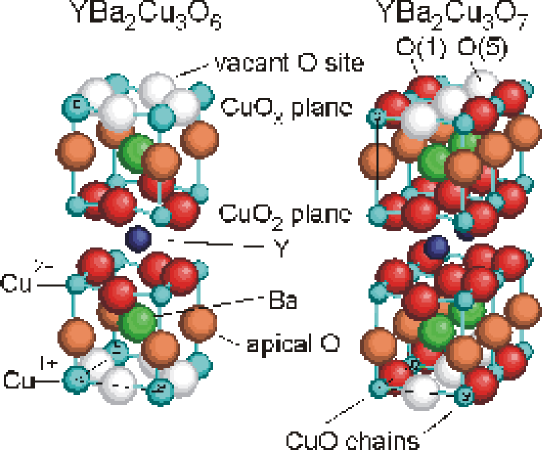
Figure 5-1: Structure of YBa₂Cu₃O_6+x. Left: one cell of tetragonal YBa₂Cu₃O₆; right: two cell of orthorhombic YBa₂Cu₃O₇. The vacant O sites in the CuO_x planes are indicated as white atoms.

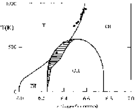
Figure 5-2: Simplified phase diagram of YBCO (from Ref. [109]).

The structural phase diagram has been mainly determined by neutron diffraction investigations [110, 23], and is shown in Fig. 5-2 in a schematic version. Numerous studies have also appeared where the phase diagram is reproduced by Monte Carlo simulations of models with different interaction energies of the O atoms up to at least the next nearest neighbors. The most successful model is the ASYNNNI (asymmetric next nearest neighbors interactions) [23, 111, 112]. Such models have also been extended to explain the hole doping in the CuO₂ planes, which depends on oxygen ordering [109] as well as content in the CuO_x planes, and are too numerous to be reviewed here. It will be sufficient to mention that they assume at least three interaction energies $V_{1}$, $V_{2}$ and $V_{3}$ for nearest, 2nd and 3rd neighboring O atoms, with $V_{1}>0$ and $V_{2}<0$ in order to reproduce the tendency to form parallel Cu-O chains, and $V_{3}>0$ in order to reproduce the O-II phase with alternately filled and empty chains.

5.2 Oxygen ordering and charge transfer between chains and planes

The mean length of the Cu-O chains may be estimated from the NQR ⁶³Cu spectra, where different peaks are found for Cu atoms which have zero, one or two neighboring O atom in the CuO_x plane, and therefore are 2, 3 or 4-fold coordinated, including the apical O atoms [113]; a quantitative analysis of the spectra therefore provides the concentrations $n_{0}$, $n_{1}$ and $n_{2}$ of such atoms. These are related with the mean chain length and degree of oxygen ordering; in fact, for infinitely long chains one has $n_{2}=x$, $n_{1}=0$, $n_{0}=1-x$, while in the limit of a small concentration of isolated O atoms one has $n_{2}=0$, $n_{1}=2x$, $n_{0}=1-2x$. The concentration and nature of the holes doped by the nonstoichiometric O^2- ions may be studied by X-ray absorption spectroscopies [114, 115], and it turns out that for $x\rightarrow 0$ Cu in the empty chains is in the Cu⁺ state, while in the CuO₂ planes it is in the Cu²⁺ state, so that the ideal undoped condition is

$$\text{YBa}_{2}\text{Cu}_{3}\text{O}_{6}=\text{Y}^{3+}\text{Ba}_{2}^{2+}\text{O}_{2}^{2-}\left(\text{Cu}^{2+}\text{O}_{2}^{2-}\right)_{2}\text{Cu}^{1+}\,;$$ (5.1)

the addition of isolated oxygen in the CuO_x planes oxidizes all the pairs of neighboring Cu atoms into the Cu²⁺ state, but chain fragments with $n>1$ consecutive O atoms would require the oxidation of $n-1$ Cu atoms to the Cu³⁺ state, which is not observed [116, 113] (see also Fig. 5-9). Therefore it may be supposed that in a first step there are $n-1$ O^1- atoms, or $n-1$ holes on the O^2- atoms in the chain; such holes may hop among the O atoms of the chain, providing a minor contribution to the electrical conductivity. This behavior may be rationalized in terms of electrostatic repulsion between the holes [117]: the repulsion between two holes on the same atom (Cu${}^{3+}=$ Cu${}^{1+}+2h^{\bullet}$) is too strong and they distribute over one O^2- and one Cu¹⁺. With increasing the chain length $n$, the electrostatic repulsion between the holes in the oxygen chain atoms drives part of them, $m$, into the CuO₂ planes where they delocalize giving rise to most of the electric conduction and superconduction. A model for the charge transfer from the chains to the superconducting planes requires the knowledge of how many $m$ holes are transferred from a chain fragment of length $n$ and has been developed by Uimin [118, 111], based also on the experimental observation that for long chains it is $m/n\sim 0.7$ [119]. For short chains of length $n=2,3$ and $4$, it has been estimated that $m=0,1,2$ holes are transferred to the planes, and the transfer proceeds with increasing $n$ up to the optimal value $m=0.7n$. For the interpretation of the anelastic spectra, it should be noted that the migration of an isolated O atom in the CuO_x plane does not change the oxidation state of the crystal, while already the formation of an oxygen pair causes the oxidation of the two neighboring Cu atoms, and the joining to longer chains involves charge transfer with the CuO₂. Therefore, the jumps of isolated O atoms are expected to be much easier than those involving the joining to or coming out of a chain fragment, since the latter involve substantial energy changes of the electronic system.

5.3 Diffusive dynamics of oxygen in the CuO_x planes

While the features of the phase diagram have been extensively studied both experimentally and theoretically, the knowledge of the diffusive and ordering dynamics of oxygen is less detailed. The macroscopic diffusion has been studied by tracer methods as recently summarized in [120], and by in- or out-diffusion in a gas atmosphere in connection with thermogravimetry or electrical resistance measurements to monitor the time dependent oxygen content [121]. The first type of experiments provides an average macroscopic diffusion coefficient, which may depend on the microstructure and possibly on inhomogeneous oxygen ordering, while the latter type of experiments is also heavily affected by the kinetics of the oxygen exchange with the gas phase and requires a model for the dependence of the electrical resistivity on the filling of the CuO_x planes. All these factors heavily influence the apparent diffusion coefficient: for example, the apparent activation energy for chemical diffusion may vary from 0.4 eV to 1 eV within the same study, depending on microstructure [122], and even more from experiment to experiment; an important role is attributed to the formation of an oxygen rich shell in each grain, that obstructs further oxygen in-diffusion during absorption experiments[122]; a surface barrier of 1.7 eV has been estimated for out-diffusion [123]. The spread of the results on oxygen diffusion in YBCO in the literature is even more impressive (several orders of magnitude) in terms of the diffusion coefficient or hopping rate at a fixed temperature. The anelastic results have the great advantage that, once identified the elastic energy loss peak due to oxygen hopping, from the condition $\omega\tau\simeq 1$ at the peak temperature, Eq. (2.30), a relaxation time $\tau$ very close to the oxygen hopping time in the bulk can be measured, even when interpreted by different microscopic mechanisms such as vacancy-assisted [124], Zener pair relaxation [125], interacting elastic dipoles [26]; in fact, different mechanisms may change the ratio between relaxation and hopping time by less than one order of magnitude. Instead, the evaluation of the local barrier for hopping depends on the type of model that is assumed, ranging from 0.68 eV for a KWW relaxation [126] to $1-1.4$ eV for Curie-Weiss interactions [127].

Figure 5-3: Comparison between the chemical diffusion coefficient of O in YBCO from various permeation experiments (a) and the hopping time of O deduced from several anelastic experiments (b). The figures are from Ref. ([121]).

5.4 Anelastic measurements of the oxygen diffusive jumps

The anelastic spectroscopy is certainly the best method to study in detail the dynamics of the mobile O atoms in the CuO_x planes. In fact, as explained in detail in Sec. 2.4.2, an anisotropic elastic dipole is associated to each O atom, which reorients by 90^o after a jump; it is then possible to selectively probe different hopping processes in different environments, through the analysis of the distinct maxima in the $Q^{-1}\left(T\right)$ curve, occurring when the condition $\omega\tau\left(T\right)=1$ is met for each process. Unfortunately, the present Thesis reports only qualitative results of the high temperature peaks, because for technical reasons the measurements were made in high vacuum, and oxygen loss occurred during the measurement of the anelastic spectra above 500 K. Therefore, the peak shapes were affected by the oxygen loss and could not be reliably analyzed in order to extract precise information on the oxygen dynamics. Still, the results clearly show the presence of two completely distinct hopping regimes: i) one that involves barriers of $\sim 1$ eV and has been studied by several authors with various techniques, ii) a much faster hopping over a barrier about 10 times smaller, that is observed only at the lowest oxygen contents.

5.4.1 Anelastic spectra at different oxygen concentrations

The anelastic spectra of YBCO change completely with varying $x$ between 1 and $\sim 0$. Figure 5-4b presents the anelastic spectra of YBCO measured at $\sim 1$ kHz at three representative values of $x$: 0.1, 0.5 and 0.9. Each of them contains a different peak; for compatibility with the labeling originally given [128, 129, 130, 131], they are called respectively P2 (at $\sim 80$ K), PH1 (at $\sim 550$ K) and PH2 (at $\sim 750$ K). All of them are thermally activated, P2 with an activation energy of 0.11 eV, and PH1 and PH2 with $E\simeq 1$ eV. The upper panel represents the CuO_x plane with $x$ increasing from left to right; the oxygen jumps causing the three main anelastic relaxation processes are put in evidence.

Figure 5-4: (a) CuO_x plane with $x$ increasing from left to right; the O jumps causing the three main anelastic relaxation processes P2, PH1 and PH2 plotted in (b) are put in evidence. The intensities of these peaks are plotted in (d) as a function of $x$, and are strongly correlated with the probabilities of the corresponding clusters plotted in (c).

Starting from the superconducting phase with $x\sim 0.9$, one finds peak PH2, which disappears on lowering $x$ and, according to the pendulum experiment of Xie et al. [124], also when $x\rightarrow 1$. For this reason those authors suggest a vacancy mechanism for the oxygen diffusion in the O-I phase, as represented in Fig. 5-4a, and associate peak PH2 with such a hopping mechanism. For $0.2<$ $x<0.8$ peak PH1 is observed, with intensity strongly dependent on thermal history; as shown later in Sec. 5.4.5, peak PH1 cannot be attributed to hopping of isolated O atoms and it must therefore be associated with jumps of oxygen aggregated into chain fragments with the exclusion of those in the ordered O-I phase, which produce peak PH2. Finally, at the lowest values of $x$ attainable, only peak P2 is observed, which is therefore associated with the jumps of isolated O atoms. Additional support to these assignments comes from the comparison between the intensities $Q_{\text{max}}^{-1}\left(x,j\right)$ of the three elastic energy loss peaks (Fig. 5-4d) and the probabilities $p\left(x,j\right)$ of the various oxygen clusters of type $j=$ P2, PH1, PH2 or nothing (Fig. 5-4c). These cluster probabilities have been reproduced from Ref. [109], where they are calculated with Monte Carlo simulations on the ASYNNNI model assuming $T=300$ K. The clusters are represented as insets in the various plots of $p\left(x,j\right)$ and labeled according to the relaxation process $j$ that they cause according to our interpretation; for PH1 the 5 clusters in the three plots have to be summed together. The $Q_{\text{max}}^{-1}\left(x,j\right)$ curves have been plotted from a large number of measurements on different samples, including EuBa₂Cu₃O_6+x, and have a considerable error both in the intensity (notice the logarithmic vertical scale) and in $x,$ since the three peaks are not always as clearly distinguishable as in Fig. 5-4b and due to uncertainties in the determination of $x$; also, the ends of the curves for $x<0.1$ and $x>0.9$ are a guess. Nevertheless, the correlation between $Q_{\text{max}}^{-1}\left(x,j\right)$ and $p\left(x,j\right)$ from Ref. [109] is excellent, for all three relaxation processes; a discrepancy can be found in the fact that $Q_{\text{max}}^{-1}\left(x,\text{P2}\right)$ is about an order of magnitude smaller than $Q_{\text{max}}^{-1}\left(x,\text{PH2}\right)$, while $p\left(x,\text{P2}\right)$ is slightly larger than $p\left(x,\text{PH2}\right)$. A possible explanation might be that the $p\left(x,j\right)$ have been calculated for $T=300$ K, while peak P2 is measured at lower temperature, where the probability of isolated O atoms should be reduced in favor of chain fragments; on the other hand, in the light of discussions in the next Sections, I think that it is too much to look for a quantitative agreement between $Q_{\text{max}}^{-1}\left(x,j\right)$ and these $p\left(x,j\right)$, and the comparison should remain on the qualitative level.

Before discussing in more detail the information obtainable from the three relaxation processes P2, PH1 and PH2, I will discuss what kind of anelastic spectra one would expect from the information presented in Sec. 2.

5.4.2 Elastic dipole of oxygen in the CuO_x plane

It is possible to estimate the elastic dipole associated with an O atom in the CuO_x plane by the $x$ dependence of the cell parameters, and it has been noted that the elastic dipole is almost independent of the oxygen content and ordering [127]. The estimate can be made by calculating the lattice parameters $a_{\text{T}}$ and $a_{\text{O}}$, $b_{\text{O}}$ of the tetragonal and orthorhombic cells in terms of the lattice parameter $a$ of the ideal oxygen-free tetragonal cell and elastic dipoles $\lambda^{\left(1\right)}$ and $\lambda^{\left(2\right)}$ of O in the sites of type 1 and 2. These sites are generally labeled as O(1) and O(5), depending whether the nearest neighbor Cu atoms are in the $y$ or $x$ direction respectively (with $x\parallel a$ and $y\parallel b$), but I will use the label 2 instead of 5. Let us indicate the components of the elastic dipole associated with oxygen as $\lambda_{1}=$ $\lambda_{xx}^{(2)}=$ $\lambda_{yy}^{(1)}$, $\lambda_{2}=$ $\lambda_{xx}^{(1)}=$ $\lambda_{yy}^{(2)}>\lambda_{1}$. The remaining component along $z$ is not interesting, since it does not change after a jump. The strain due to the occupation of the $n_{1}+n_{2}=x$ sites is

$$\varepsilon_{ij}=n_{1}\lambda_{ij}^{(1)}+n_{2}\lambda_{ij}^{(2)}$$ (5.2)

and the cell parameters in the O and T phases, assuming $n_{1}^{\text{(O)}}=x_{\text{O}}$, $n_{2}^{\text{(O)}}=0$ and $n_{1}^{\text{(T)}}=n_{2}^{\text{(T)}}=x_{\text{T}}/2,$ are:

$$a_{\text{T}} =a\left[1+x_{\text{T}}\frac{1}{2}\left(\lambda_{1}+\lambda_{2}\right)\right]$$ (5.3)

$$a_{\text{O}} =a\left[1+x_{\text{O}}\lambda_{1}\right]\,,\quad b_{\text{O}}=a\left[1+x_{\text{O}}\lambda_{2}\right]$$ (5.4)

from which one deduces

$$a =\frac{a_{\text{T}}x_{\text{O}}-\frac{1}{2}\left(a_{\text{O}}+b_{\text{O}}\right)x_{\text{T}}}{x_{\text{O}}-x_{\text{T}}}$$ (5.5)

$$\left(\lambda_{2}-\lambda_{1}\right) =\frac{b_{\text{O}}-a_{\text{O}}}{x_{\text{O}}a}$$ (5.6)

$$\left(\lambda_{1}+\lambda_{2}\right) =\frac{b_{\text{O}}+a_{\text{O}}}{x_{\text{O}}a}=\left(\frac{a_{\text{T}}-a}{a}\right)\frac{2}{x_{\text{T}}}$$ (5.7)

In the following table I consider the cell parameters measured by neutron diffraction in two tetragonal and two orthorhombic samples in Ref. [132], and two pairs of data taken from Fig. 5 of Ref. [110].

$$x_{\text{T}}$$ (Å) (Å) (Å) Ref. (Å)

0.18 0.96 (O-I) 3.8587 3.8227 3.8872 [132] 3.8596 0.0174 -0.0012

0.18 0.78 (O-III) 3.8587 3.8265 3.8875 [132] 3.8592 0.0203 -0.00073

0.25 0.96 (O-I) 3.8586 3.8227 3.8872 [132] 3.8599 0.0174 -0.0013

0.25 0.78 (O-III) 3.8586 3.8265 3.8875 [132] 3.8591 0.0203 -0.00069

0.095 0.93 3.8600 3.8227 3.8872 [110] 3.8606 0.0180 -0.0016

0.28 0.93 3.862 3.8227 3.8872 [110] 3.8650 0.0179 -0.0028

The sample with $x_{\text{O}}=0.78$ was detwinned and showing O-III superstructure (one filled chain every three) and the authors report negligible occupancy of O(5) in the ortho phases; therefore it should be meaningful to assume $n_{1}^{\text{(O)}}=0$ also for such a relatively low value of $x$. From these data it can be concluded, in accordance with Ref. [127], that $\left(\lambda_{2}-\lambda_{1}\right)\simeq 0.019\pm 0.0015$ and $\frac{1}{2}\left(\lambda_{1}+\lambda_{2}\right)\simeq-0.0018\pm 0.0001$.

An important remark must be made on this type of derivation of the elastic dipole of oxygen in the CuO_x planes: it is valid for oxygen aggregated into chains or chain fragments, but not necessarily for isolated O atoms; in fact, in Sects. 5.4.6-5.4.8 it will be shown that around room temperature and below, the concentration of isolated O atoms is very small also in highly oxygen deficient samples. As explained in those Sections and in Sec. 5.2, the state of aggregated and isolated O atoms is different, due to charge transfer effects dependent on the chain length, and it is not obvious that the elastic dipole of an isolated O atom should be the same as that of an oxygen belonging to a chain. Therefore, it is not obvious that the value of the anisotropy $\Delta\lambda=0.019$ found above is appropriate for evaluating the anelastic relaxation from oxygen hopping.

Let us see if it is compatible with the peak intensities reported in Fig 5-4. In Appendix B is calculated an estimate of the relaxation strength for the Young’s modulus of an isotropic polycrystal; neglecting porosity, it should be

$$\Delta=\frac{1}{15}\frac{cv_{0}}{k_{\text{B}}T\,\left\langle E^{-1}\right\rangle}\left(\lambda_{1}-\lambda_{2}\right)^{2}\,\,,$$ (5.8)

where $c$ is the concentration of relaxing dipoles. The Young’s modulus of ceramic YBa₂Cu₃O_6+x corrected for porosity has been estimated as $E=90$ GPa and 125 GPa for low and high $x$, respectively [133, 134]. Setting $E=100$ GPa, $\rho\simeq 6.3$ g/cm³, $v_{0}=175\times 10^{-24}$ cm³ we get

$$\Delta\sim\frac{30~{}\text{K}}{T}c\,.$$ (5.9)

If we want to compare with the height of peak PH2 we set $T\sim 750$ K and $c\sim 0.1$, since according to the vacancy mechanism [124] the intensity is proportional to the O vacancies in the O-I phase and not to $x\simeq 0.9$; it turns out $Q_{\text{max}}^{-1}=\frac{\Delta}{2}\sim 2\times 10^{-3}$, instead of the observed $10^{-2}-10^{-1}$ (Fig. 5-4). The intensity however, might be enhanced by the proximity to the ordering transition [127], by a Curie-Weiss like factor; from the YBCO phase diagram (Fig. 5-2) it appears that at $x\sim 0.9$ the transformation to the tetragonal phase, if any, is at $T>1000$ K, and therefore $T=750$ K in the denominator should be substituted with $T-T_{\mathrm{C}}>250$ K, which does not change much the situation. It seems therefore that $\Delta\lambda=0.019$ is too small for explaining the large relaxation strength we observe for peak PH2, but these estimates are really rough. In any case, it is difficult to draw quantitative conclusions on the elastic dipole of oxygen from the anelastic spectra, because, when measuring peaks PH1 and PH2 at high temperature, one has oxygen loss during the measurement, while for peak P2 one needs an independent estimate of the concentration $c$ of free oxygen.

5.4.3 Interactions among the oxygen atoms in the Bragg-Williams approximation

As explained in detail in Sec. 2.4, Wipf and coworkers performed aftereffect [135, 26, 127] experiments on YBCO and took into account the interactions among elastic dipoles in the Bragg-Williams approximation, analogous to the Curie-Weiss approximation above $T_{\mathrm{C}}$. They showed that the anelastic aftereffect (the time dependence of strain after application of a constant stress) for $x\simeq 0.4$ around 380 K presents an enhancement of the relaxation strength and time by a factor $T/\left(T-T_{\mathrm{C}}\right)^{-1}$, where $T_{\mathrm{C}}$ is the temperature below which the elastic dipoles associated with the O atoms start ordering themselves, namely the temperature of the T/O phase transformation. Around 380 K, a critical concentration $x_{c}\simeq 0.45$ is found, where both the relaxation strength $\Delta\left(x\right)$ and relaxation time $\tau\left(x\right)$ are enhanced by at least a factor 10 over the values found away from $x_{c}$ [127]. The value $x_{c}\simeq 0.45$ is somewhat higher than $x\sim 0.3-0.4$ deduced from the O-T line of the experimental phase diagram [109, 136].

The elastic interaction alone cannot be the origin neither of the tetragonal to orthorhombic transition nor of the several orthorhombic phases, which are mainly determined by short range interactions of electronic origin, as schematized in the ASYNNNI model. In fact, if one assumes that the ordering temperature is given by $k_{\text{B}}T_{\mathrm{C}}=\alpha\frac{x}{2}\left(1-\frac{x}{2}\right)$[see eq. (8.3)] and tries to fit the O-T boundary of YBCO with such $T_{\mathrm{C}}\left(x\right)$, one obtains $\alpha/k_{\text{B}}=2500-4000$ K, as shown in Fig. 5-5, On the other hand, Wipf [137] estimated the elastic contribution to $\alpha$ as $\alpha^{\text{el}}/k_{\text{B}}\sim 290$ K, which is an order of magnitude smaller than the value needed to reproduce the observed ordering temperatures.

Figure 5-5: Fit of the tetragonal/orthorhombic boundary with $T_{\mathrm{C}}\left(x\right)$.

Therefore, a treatment of the interaction among the O atoms in the mean field approximation, as presented in Sec. 2.4, is not fully consistent if the main contribution to the interaction parameter $\alpha$ is of local electronic origin; still, it is useful to reproduce important effects in the relaxation strength and rate of the anelastic peaks due to oxygen hopping, as shown by their critical enhancement observed in after-effect experiments [127].

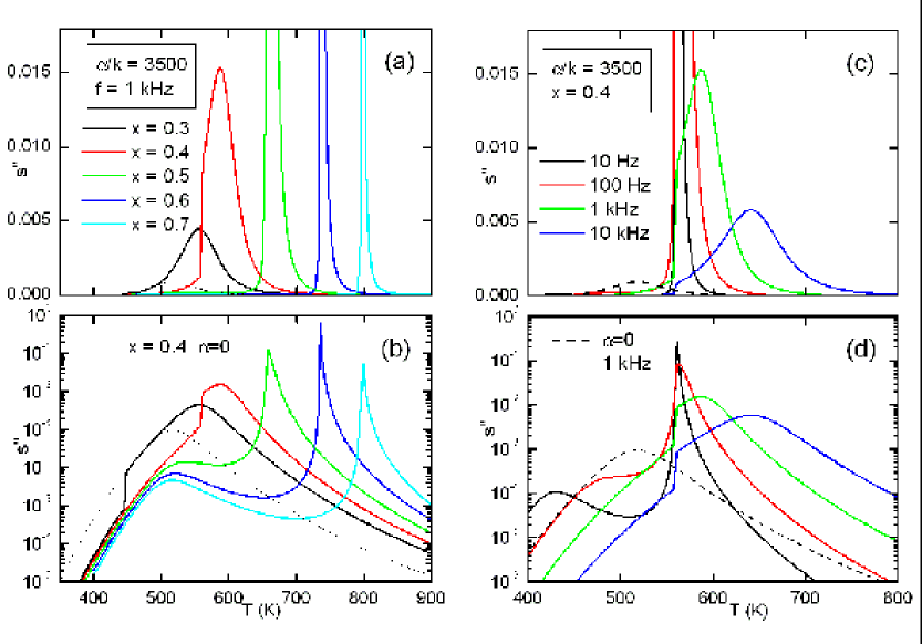
Figure 5-6: $s^{\prime\prime}\left(\omega,T\right)$ curves in logarithmic (upper) and linear (lower) scales calculated in the Bragg-Williams approximation with $\tau_{0}=10^{-13}$ s, $E/k=11000$ K and $\omega/2\pi$, $x$ and $\alpha$ as indicated in the legends.

According to the phase diagram of YBCO (Fig. 5-2), on varying $x$ the temperature $T_{\mathrm{C}}\left(x\right)$ of the T/O-I ordering transition crosses at $x\sim 0.5$ the temperatures of peaks PH1 and PH2. Then, it would be interesting to evaluate the effect of this ordering transition, at least in the simple Bragg-Williams approximation presented in Sec. 2.4. Above $T_{\mathrm{C}}$, the simple Curie-Weiss-like formula (2.50) can be used, but below $T_{\mathrm{C}}$ one has to calculate the expressions (2.72) and (2.78), or equivalently the order parameter $\xi=\frac{1}{2}\left(c_{1}-c_{2}\right)$. In Appendix A numerical approximations are provided for $\xi\left(c,T\right),$which might be useful for fitting purposes. As already noted, our data are generally not susceptible to reliable analysis, since oxygen loss occurred during the measurements, therefore I simply plot in Fig. 5-6 some $s^{\prime\prime}\left(\omega,T\right)$ curves calculated according to Eqs. (2.72), (2.78) with the approximations (8.5), (8.6). The curves are plotted in linear (upper panels) and logarithmic (lower panels) scales as a function of $x$ in (a) and (b) and as a function of frequency in (c) and (d); the relaxation time in the absence of interaction has been chosen as the typical hopping time of O, $\tau=10^{-13}$ s $\exp\left(11000/T\right)$, the interaction parameter $\alpha/k_{\text{B}}$ has been chosen as 3500 K, in order to have the transition in the correct temperature range, and also plotted as a dashed line is the reference peak with $\alpha=0$ (no interaction) at $T_{p}=520$ K (for 1 kHz). The ordering transition on cooling is clearly visible as a narrow peak, when $T_{\mathrm{C}}>T_{p}$ and as a drop of intensity when $T_{\mathrm{C}}<T_{p}$. Although the anelastic spectra we measured for $x<0.5$ contain some narrow peaks clearly due to oxygen ordering transitions [138], there is no clear relationship with the curves calculated in Fig. 5-6 and it is evident that a more complete treatment of the short range interactions, like in the ASYNNNI model, is necessary to describe the high-temperature anelastic spectra of YBCO.

5.4.4 Hopping in the O-I phase - peak PH2

The information obtainable on PH2 from the present measurements is only limited to the observation that it is a process occurring in the O-I phase, distinct from PH1; in fact, the experiments are made in vacuum and rapid oxygen loss occurs during the measurement, affecting both shape and intensity of the peak. More reliable measurements of this process have been made by other authors with the pendulum [124], which allows some O₂ pressure to be maintained around the sample and moreover lowers the peak temperature. The mechanism devised for PH2 in Fig. 5-4 is the one requiring a neighboring vacancy, as suggested by Xie et al. [124], on the basis of fact that its intensity vanishes for $x\rightarrow 1$. That analysis, however, is not fully consistent, since it assumes an asymmetry between the energies in sites O(1) and O(5), $\Delta E\left(x\right)=E_{5}-E_{1}$, which is maximum for $x=1$ and decreases to 0 when the sample becomes tetragonal. Such an asymmetry energy was taken into account for reproducing the decrease of the apparent activation energy with decreasing $x$, but it was not considered that it would also reduce the intensity of the peak, due to the depopulation factor in Eq. (2.15), thereby accounting for a consistent part of the reduction of the peak intensity when $x\rightarrow 1$.

Among other measurements of peak PH2 [125, 139, 126], I would like to signal isothermal spectra measured with the pendulum [140] that confirmed the presence of two peaks, the one at higher temperature is associated with the orthorhombic phase and should therefore correspond to PH2, while the other one to PH1. This confirmation is important, since it is based on stationary and reproducible spectra.

5.4.5 Other jumps of aggregated oxygen and oxygen ordering - peak PH1

Figure 5-7a (from Ref. [130]) shows peak PH1 measured in an EuBa₂Cu₃O_6+x, which has anelastic spectra and all the physical properties very similar to YBa₂Cu₃O_6+x. The peak with higher intensity is for $x\simeq 0.5$, and proceeding with the outgassing treatments it decreases in intensity and shifts to higher temperature; the effective activation energy, estimated from the shift of the peak at higher frequency, also increases from 1.1 to 1.3 eV. While the decrease in intensity is easy to understand after the considerations of Sec. 5.4.1, the increase in activation energy has no obvious explanation.

Figure 5-7: (a) Peak PH1 measured in EuBa₂Cu₃O_6+x starting from $x\simeq 0.5$; with decreasing $x,$the peak decreases in intesity and shifts to higher temperature. (b) After quenching to room temperature from 990 K, peak PH1 is strongly depressed, but reappears with aging at high temperature.

Figure 5-7b shows another interesting effect, which excludes the hopping of isolated O atoms as possible mechanism for peak PH1. Curve #1 has been measured on heating after quenching from 990 K to room temperature in few seconds, by pouring water on the quartz tube where the sample was heated. After such a quenching the concentration of isolated O atoms should be maximum, but peak PH1 is strongly depressed, and instead a small peak appears near 480 K. The latter does not shift in temperature with increasing frequency and is therefore signalling the occurrence of an ordering transition near 480 K, like the frequency independent peak at 560 K in the curves of Fig. 5-6d; it is difficult to say whether the ordering occurring above 480 K is simply a lengthening of the Cu-O chains or the formation of O-II domains. It is clear however, that peak PH1 is due oxygen jumps within such long chains or domains and not to isolated O atoms or even pairs or very short chains, which are promptly formed. In fact, the peak develops with thermal cycling above 500 K (curves 2 and 3), and the increase of intensity cannot be attributed to oxygen uptake, since the measurements are made in high vacuum.

We also observed additional frequency independent anomalies up to 580 K [138], which appear only on heating and not on cooling (as for curve 3 in Fig. 5-7b), but still there is no better explanation than some types of ordering transitions. This complex phenomenology demonstrates that situation is even more complex than it appears from the diffraction measurements of oxygen ordering.

5.4.6 Isolated oxygen atoms - peak P2

There is extensive evidence that the effective barrier for the diffusive jumps of the O atoms in the CuO_x planes is of the order of $1$ eV, as discussed in the previous Sections. It should be noted, however, that none of the high temperature $Q^{-1}\left(T\right)$ peaks presents the dependence on $x$ expected from the hopping of a concentration $c=x/2$ of an interstitial species (if one regards oxygen in the CuO_x plane as an interstitial species, and takes into account that there are 2 sites available for each Cu atom). As a matter of fact, none of the behaviors expected from an interstitial solution is observed; e.g. the proportionality of the relaxation strength to $c$ in the high dilution limit, or to $c\left(1-c\right)$ if one takes into account the filling of a finite number of sites [13], or to $c^{2}$ or some other power of $c$ if interstitial complexes contribute. This is due to the strong interaction between the O atoms, and the difficulty of probing the two limits $x\rightarrow 0$ and $x\rightarrow 1$. The interaction among the O atoms is so strong to prevent the filling of the planes above $c=0.5$ (or $x=1$). That concentration corresponds to the O-I phase, with completely filled chains, and can be approached but probably never obtained. We attempted at reaching the high dilution limit $x\rightarrow 0$, but this also cannot be done, due to the decomposition of YBCO in vacuum at high temperature into the more stable oxides. Bormann and Nölting [141] found the decomposition limit $p\left(T\right)$ below which YBa₂Cu₃O_6+x transforms into the more stable oxides Cu₂O, BaCuO₂ and Y₂BaCuO₅ (the latter easily recognizable from the green color), and found that the lowest attainable oxygen content is YBa₂Cu₃O_6.05.

The first anelastic measurements on highly outgassed YBCO [128, 142] showed a rather unexpected result: all the relaxation processes at high temperature were completely suppressed [142] and a new intense peak, labeled P2, appeared around 60 K, close to a Debye relaxation with an activation energy of 0.11 eV [128] (see also Fig. 5-4). Since oxygen was certainly present in the CuO_x planes at the level of several molar percent also after outgassing, the most obvious conclusion was that P2 is due to hopping of isolated O atoms. This is striking, since the barrier for jumps of isolated O atoms would be 10 times lower than that for jumps of oxygen within chains, and also in any other known oxide; such a low barrier is rather comparable that for interstitial H in bcc metals. In fact, the same relaxation process has been observed also in NQR experiments and attributed to polaron hopping [143]. Even accepting that the O atoms in the nearly empty CuO_x planes overcome a barrier as little as 0.1 eV to perform a diffusive jump, some difficulties arise in conciliating such a high mobility with the long time required for oxygen to reach an equilibrium configuration; this led de Brion et al. [144] to assign P2 to hopping of isolated O atoms trapped by some defect, e.g. a vacancy in the apical oxygen sublattice. It has later been argued [145] how peak P2 is more likely to be due to oxygen rather than small polaron hopping, considering that its activation energy is independent on concentration, and how it is possible that the extremely fast mobility of isolated O atoms may coexist with a slow kinetics for reaching equilibrium.

Part of the following results appeared in Ref. [145]. We approached the $x\rightarrow 0$ limit by heating the samples in a vacuum of $\sim 10^{-5}$ mbar at progressively higher temperatures (up to 1000 K) for $\sim 2$ h. The last outgassing treatment at 1000 K was slightly beyond the decomposition limit, and traces of superficial green phase had to be removed with emery paper. The oxygen content after the final outgassing treatment was estimated from the $c$ lattice parameter by X-ray diffraction, and was found $x=0.05\pm 0.05$, in agreement with the results on the YBCO stability [141]. Figure 5-8a shows the evolution of peak P2, starting with $x\gtrsim 0.4$ (curve 1); where the peak is practically absent, and peak P3 at 90 K (8 kHz) is still visible; the peak appears after outgassing up to 810 K (curve 2), with $x\sim 0.3$, increases after 2 h in vacuum at 980 K (curve 3), and starts decreasing with further outgassing (curve 4 after additional 2 h at 1000 K) or after long aging at room temperature (curve 5 after 13 months).

Figure 5-8: (a) development of peak P2 with outgassing and aging at room temperature; (b) fits of peak P2 measured at two frequencies in the states corresponding to curves 2 and 5 in (a).

The characteristics of peak P2 other than the intensity are practically independent of $x$ or sample history, indicating relaxation of some simple point defect. Figure 5-8b shows fits to the peak measured at two vibration frequencies (0.7 and 9 kHz) in the states with the highest and lowest intensity (curves 3 and 5 of Fig. 5-8a). For peak P2 the Cole-Cole expression (2.45) was found to provide a slightly better interpolation than the Fuoss-Kirkwood one, and it has been allowed for relaxation between slightly inequivalent sites [Eqs. (2.15) and (2.22b) with $\Delta E\neq 0$], in order to reproduce the fact that the peak intensity is slightly larger at higher temperature, instead of exhibiting $1/T$ behavior (see the discussion at the end of Sec. 2.0.1). Therefore peak P2 has been interpolated with

$$Q^{-1}\left(T\right) =\frac{\Delta_{0}}{2T\cosh^{2}\left(\frac{\Delta E}{2k_{\text{B}}T}\right)}\frac{\sin\left(\frac{\pi}{2}\alpha\right)}{\cosh\left[\alpha\ln\left(\omega\tau\right)\right]+\cos\left(\frac{\pi}{2}\alpha\right)}$$ (5.10)

$$\tau =\tau_{0}e^{E/k_{\text{B}}T}/\cosh\left(\frac{\Delta E}{2k_{\text{B}}T}\right)$$ (5.11)

plus a linear background and a small contribution from peak P3 around 90 K. The peak may be fitted with $\tau_{0}=1.5\times 10^{-13}$ s , $E/k_{\text{B}}=1290$ K, $\alpha=0.84$ and $\Delta E\simeq 130$ K in all cases, except for the final state (curve 5), where the slightly different values $\tau_{0}=4\times 10^{-14}$ s and $E/k_{\text{B}}=1370$ K give a better interpolation. The slight shift of the peak temperature from curve 2 to curve 5 is due to changes of the resonance frequency of the sample. It can therefore be concluded that the relaxation parameters of peak P2 are independent on $x$ and sample conditions within experimental error.

5.4.7 Isolated and aggregated oxygen atoms

The first question to answer is how is it possible that the oxygen jumps for $x<0.3$ occur over a barrier about 10 times smaller than for $x>0.3$. The proposed explanation is that there are two substantially different types of jumps: fast jumps of isolated O atoms, and slow jumps, occurring at high values of $x$, that involve breaking and formation of chemical bonds with a neighboring O atom. Therefore, the real barrier for oxygen hopping in the CuO_x planes would be the one of peak P2, 0.11 eV, while the additional 0.9-1.0 eV are due to the formation of chemical bonds and, as we shall see later, to the electrostatic interaction between neighboring O atoms. This hypothesis is reasonable in view of the model for the hole states and charge transfer from chains to planes presented in Sec. 5.2, where it has been pointed out that: i) jumps of isolated O atoms do not affect the electronic state; ii) the formation (or dissolution) of a pair of nearest neighbor O atoms involves the change of a hole of Cu^3d character into O^2p, with a higher energy (but lower than having two holes on a same Cu¹⁺ atom); iii) jumps to or from longer chains involve charge transfer between chain and CuO₂ plane.

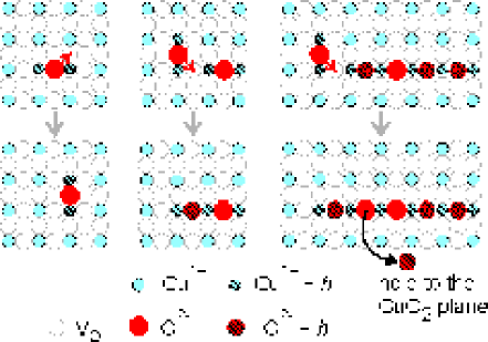
Figure 5-9: Effect of different types of O jumps in the CuO_x plane on the holes. From left to right: 1) no change for an isolated O atoms; 2) a Cu^3d hole is converted into a O^2p hole with higher energy; 3) after the formation of a longer chain, a hole is pushed to the CuO₂ planes.

Figure 5-9 presents a sketch of these processes. From these considerations it appears that only the jumps of isolated O atoms involve only a simple reorientation of the elastic dipole, as in the Snoek effect, while all other types of jumps, besides a higher effective barrier, should also present different initial and final energies, and possibly elastic dipoles. The energies for creating a hole or changing its state are of the order of several tenths of eV, which means thousands of kelvin in the temperature scale. From Sec. 2.0.1 it appears that in such cases the depopulation factor makes the relaxation strength strongly increasing with temperature, and this should be easily noted as a peak whose intensity is higher when measured at higher frequency, instead of being smaller by the $1/T\;$factor. The anelastic data at high temperature collected by us do not evidence clearly such a behavior, even though the oxygen loss occurring during the measurement in vacuum does not make this observation very reliable.

Figure 5-10: Jumps of an O atom between terminals of two perpendicular chains of similar length leaves the hole state unaffected.

A possible explanation for this fact would be that the anelastic relaxation observable at high temperature is due to those jumps between Cu-O chains that do not change the overall hole state, and therefore whose initial and final electronic energies are the same. Figure 5-10 presents the example of a jump between the ends of two perpendicular chains. If both chains have $n<5$, no hole will be transferred to or from the planes after the jump, at least according to Uimin’s model [118, 111]; also, if their length is similar, then the total count of the various types of holes will be the same before and after the jump. Jumps of this type, although involve a high activation energy for the temporary change of the electronic configuration, do have the same initial and final energy, and therefore the related relaxation strength is proportional to $1/T$, as usual. It should be noted that this type of jumps is probably involved in the motion of twins. Considering that the hopping energy or bandwidth of the holes is $\sim 0.4$ eV [117], it is likely that the difference between initial and final energy of a jump that changes the electronic state is of the order of tenths of eV; already setting $\Delta E=0.2$ eV in Eq. (2.15) the depopulation factor $\cosh^{-2}\left(\Delta E/2k_{\text{B}}T\right)$ reduces the relaxation strength by 25 times at 500 K, a temperature where the peaks due to the chain rearrangements are observed. These considerations have been overlooked up to now in all anelastic studies of the oxygen jumps, which implicitly assume the equivalence between the electronic energy before and after the oxygen jump. A reliable analysis of such processes should take into account the energies involved in the rearrangements of the chains and the statistical weights of the various chain configurations; this is outside the scope of the present investigation, in view of the impossibility of measuring a stable anelastic spectrum in vacuum at high temperature.

5.4.8 Slow achievement of equilibrium and expected concentration of isolated oxygen atoms

The mobility of the isolated O atoms deduced from peak P2 is extremely fast, and corresponds to $10^{11}$ jumps per second at room temperature. With such high a mobility one expects an almost instantaneous achievement of the equilibrium configuration of the O atoms, contrary to observations. In fact, oxygen ordering at room temperature may proceed for months both at high and low values of $x$. A well known example is the fact that if a sample with relatively low $x$ is quenched to room temperature, its superconducting temperature is found to increase of over 10 K with aging at room temperature over periods of days [146]; this is attributed to slow reordering of oxygen at room temperature, with consequent change of the concentration of holes injected in the CuO₂ planes and change of $T_{\mathrm{c}}$. Another example is the slow decrease of the intensity of peak P2 with aging at room temperature, which can be attributed to a slow decrease of the number of the isolated O atoms at room temperature and below. The discrepancy between the supposed fast hopping rate of the isolated O atoms and the slow reordering kinetics has been put in evidence by de Brion et al. [144] with the following simple argument. In the low $x$ limit and assuming that only O pairs are formed, the authors assumed that the time for reaching equilibrium, $t_{\text{eq}}$, is the time for forming pairs starting from a random distribution of isolated (free) O atoms; therefore they obtain $t_{\text{eq}}\sim\tau_{f}/x^{2}$, where $\tau_{f}$ is the mean hopping time of the free O atoms and $x$ their concentration. The extrapolation of $\tau$ from peak P2 to room temperature yields $\tau_{f}\sim 10^{-11}$ s, which would require $x\sim 10^{-8}$ for obtaining $t_{\text{eq}}\sim 1$ day and $x\sim 5\times 10^{-10}$ for extending $t_{\text{eq}}$ to 1 year, as we observed. Such concentrations are of course unrealistic, being $x>0.1$, and this fact induced de Brion et al. to attribute peak P2 to hopping of oxygen trapped by some defect, or to the reorientation of O pairs, leaving $\tau_{f}\sim\tau_{a}=\tau_{0}\exp\left(E_{a}/k_{\text{B}}T\right)$, the usual hopping time for aggregated oxygen with a barrier of $E_{a}\sim 1$ eV. A flaw in this argument is the assumption that equilibrium is reached once all the O atoms have had the opportunity of forming a pair or chain fragment for the first time. This is not true, since the process of reaching equilibrium will require further steps of dissociation and aggregation of the chain fragments in the intermediate metastable configurations, and these require jumps with the characteristic time $\tau_{a}$ of the aggregated oxygen; in conclusion, the limit steps are those with $\tau_{a}$.

The picture of only two hopping times, $\tau_{f}=\tau_{0}\exp\left(E_{f}/k_{\text{B}}T\right)$ with $E_{f}=0.11$ eV for hopping of isolated O atoms and $\tau_{a}=\tau_{0}\exp\left(E_{a}/k_{\text{B}}T\right)$ with $E_{a}\simeq 1$ eV for leaving a chain fragment or diffusing between chains (see Fig. 5-11a), is nevertheless inadequate. In fact, the rate equation for the equilibrium between free and aggregated O, in the simplest form and neglecting any geometrical factor, would be

$$\frac{dc_{f}}{dt}\simeq\frac{c_{a}}{\tau_{a}}-\frac{c_{f}}{\tau_{f}}x\,,$$ (5.12)

where $x$ is the probability that the jump of the free O atom joins another O atom. By posing the condition of stationarity and recalling that $c_{a}+c_{f}=x$ and $\tau_{a}\gg\tau_{f}$, one obtains for the equilibrium concentration of free oxygen

$$\overline{c}_{f}=\frac{x\tau_{f}}{x\tau_{a}+\tau_{f}}\simeq\frac{\tau_{f}}{\tau_{a}}=\exp\left(\frac{E_{f}-E_{a}}{k_{\text{B}}T}\right)=\exp\left(\frac{-E_{b}}{k_{\text{B}}T}\right)\,,$$ (5.13)

which is of the order of $10^{-15}$ at room temperature with a binding energy $E_{b}=E_{a}-E_{f}\simeq 0.9$ eV. We find again that the concentration of free O would be negligible at room temperature and below, while peak P2 requires $c_{f}\sim 10^{-4}$ below 100 K.

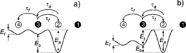
Figure 5-11: Potential felt by an isolated O atom (3) on approaching another O atoms (1) in site 2. In (a) only the binding energy $E_{b}$ of the pair is taken into account; in (b) also the electrostatic repulsion is considered.

The explanation for this apparent inconsistency also explains why peak P2 is not observed at $x>0.4$. In fact, it is proposed that the electrostatic repulsion between the O^2- ions, which is effectively screened in the conducting phase by the mobile holes, becomes strong in the semiconducting phase, with $x<0.4$; the result is an increase of the saddle point, as shown in Fig. 5-11b. The electrostatic energy of the two O atoms in the saddle point configuration between second and first neighboring positions is $q^{2}\times 0.6$ eV, where $q$ is the effective oxygen charge, $q\simeq-2$, without taking into account any screening. It is an energy 2.5 larger than $E_{a}$, and this demonstrates the importance of screening in determining the short range interaction between the O atoms. If the saddle point between sites 3 and 2 is larger than that between two free sites 3 and 4, than we have to introduce a ”trapping” activation energy $E_{t}$ for the pair formation, and $E_{b}$ becomes $E_{a}-E_{t}$, where $E_{t}$ is not known but can be a large fraction of $E_{a}$. The new picture is that of a generally metastable concentration $c_{f}$ of free O atoms that is small at room temperature and below, but larger than the equilibrium $\overline{c}_{f}$, unless very prolonged aging over years occurs after the last excursion to high temperature. These free O atoms jump with an extremely fast mean time $\tau_{f}$ and therefore approach continuously other O atoms and chain fragments; the mean time for aggregating with other O, however, is the much longer $\tau_{t}=\tau_{0}\exp\left(E_{t}/k_{\text{B}}T\right)$, at least in the semiconducting regions. This fact maintains the concentration of excess free O rather stable, making perfectly reasonable the observation of peak P2. In this respect, it should also be noted that the concentration of free O atoms at the peak temperature $T_{p}\simeq 65$ K is not $\overline{c}_{f}\left(T_{p}\right)$, but much closer to the starting room temperature value $c_{f}^{0}\left(\text{RT}\right)\geq\overline{c}_{f}\left(\text{RT}\right)$. In fact, assuming that the starting metastable room temperature value $c_{f}^{0}\left(\text{RT}\right)$ is determined by the longer hopping time $\tau_{a}$, during cooling, $\overline{c}_{f}\left(T\right)$ will be approached with the faster characteristic time $\tau_{t}$, but for a measuring run with a cooling rate of the order of 1 K/min, $c_{f}$ will remain frozen when $\tau_{t}$ reaches $\sim 10$ min, therefore above $\overline{c}_{f}\left(T^{*}\right)$, where $\tau_{t}\left(T^{*}\right)=10$ min. I do not know of any experimental indication of $E_{b}$, but a range of values sufficient to freeze $c_{f}\sim 10^{-4}$ necessary for observing peak P2 can be estimated setting $10^{-4}\simeq\overline{c}_{f}\left(T^{*}\right)\simeq\exp\left(\frac{-E_{b}}{k_{\text{B}}T^{*}}\right)$ and $10$ min$\,=\tau_{t}\left(T^{*}\right)=\tau_{0}\exp\left(\frac{-E_{t}}{k_{\text{B}}T^{*}}\right)$ with the constraint $E_{b}+E_{t}=E_{a}\simeq 1$ eV. It results that for $0.2~{}$eV$\,<$ $E_{b}<$ $0.3$ eV one freezes $10^{-5}<\overline{c}_{f}\left(T^{*}\right)<10^{-4}$ around 250 K$\,<T^{*}<$ 280 K.

At last, we note that in the proposed picture, at room temperature and below, the rearrangement of the aggregated O atoms is extremely slow ($\tau_{a}\left(290~{}\text{K}\right)\simeq 6$ h) and a minor concentration of highly mobile O atoms remains, that are bound to diffuse in the semiconducting regions free of O chains. Since their mean hopping time $\tau_{f}$ is much faster than the mean time for joining other O atoms, $\tau_{t}$, being $\tau_{f}/\tau_{t}=\exp\left[\left(E_{f}-E_{t}\right)/k_{\text{B}}T\right]>10^{2}$, they can be considered as effectively free from the strong interactions giving rise to the ordered phase and described in Sects. 2.4 and 5.4.3. In fact such interactions involve changes of the great majority of aggregated O, which is frozen on the time scale of $\tau_{f}$. It is therefore consistent to ignore any ordering temperature $T_{\mathrm{C}}$ in eq. (5.10). The introduction of a mean asymmetry $\Delta E$ $\simeq 130$ K between the free sites is justified by the fact that the regions free of O pairs and chains, where the isolated O atoms diffuse, are certainly small and their site energies are strongly perturbed by strain due to the surrounding aggregated O. This effect is particularly evident for defect relaxation with small activation energy, giving rise in this case to $\Delta E/E=0.1$, but is unnoticed for the high temperature relaxation with $\Delta E/E=0.01$. The magnitude of $\Delta E$ is typical of the site energy shifts due to strain interactions, as discussed in the end of Sec. 2.0.1.

5.5 Motion of oxygen in off-center positions of the Cu-O chains

The low temperature anelastic spectrum of well oxygenated YBCO is shown in Fig. 5-12 and presents three peaks, which we label P1, P3 and P4, with activation energies of 0.11, 0.16 and 0.19 eV respectively [147]. Peak P1 will be dealt with in the next section.

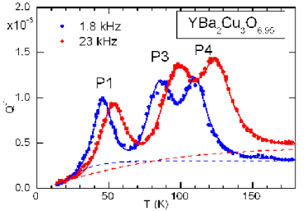
Figure 5-12: Low temperature elastic energy loss of YBCO measured at 1.8 and 23 kHz. The continuous lines are a fit as explained in the text with the dashed lines as background.

The continuous lines in Fig. 5-12 are a fit with the Fuoss-Kirkwood expression (2.42) for peaks P3 and P4 and (2.48) for P1 plus a background of the form $\tanh\left[\left(T-T_{0}\right)/w\right]$ (dashed lines). Again, in order to reproduce the intensities of the peaks at both frequencies with the same set of parameters it is necessary to introduce the possibility that relaxation occurs between energetically non-equivalent states. This requirement is normal in such a disordered system like YBCO at temperatures below 100 K (see the end of Sec. 2.0.1). It is therefore necessary to introduce a correction of the type $\cosh^{-2}\left(\Delta E/2k_{\text{B}}T\right)$ to the relaxation strength and $\cosh^{-1}\left(\Delta E/2k_{\text{B}}T\right)$ to the relaxation time (Eqs. (2.15) and (2.22b)). The parameters used for the fit are reported in the table.

peak $$E/k_{\text{B}}$$ (K) (K) (s)

P1 908 61 0.29 .57

P3 1730 186 0.49

P4 2450 211 0.79

The pre-exponential factors $\tau_{0}$ are all compatible with point defects, while the activation energies of P3 and P4, 0.15 and 0.21 eV, are very close to those deduced from the condition $\omega\tau=1$ at the maxima of the peaks measured by several authors in a broad range of frequencies, 0.16 and 0.19 respectively [147]. The peaks are also considerably broader than pure Debye relaxations, and the asymmetry parameters $\Delta E$ are within 10% of the activation energy; they do not affect much the other parameters but definitely improve the fit. The evolution of peaks P3 and P4 with doping is shown in Fig. 5-13: after an outgassing treatment to $x\sim 0.5$, as deduced from resistivity (absence of superconductivity down to 70 K and increase of resistivity by 20 times at room temperature), peak P4 was almost suppressed, while P3 slightly enhanced. The broad peak at 220 K seems to be connected with some type of oxygen ordering, as briefly discussed in Sec. 5.7.

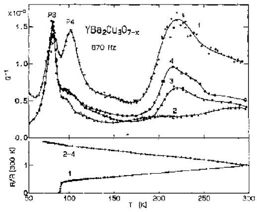
Figure 5-13: Elastic energy loss and resistance normalized to room temperature of an YBCO sample with $x\simeq 0.95$ (curves 1) and after outgassing to $x\sim 0.5$ (curves 2-4) [from [147]].

The existence of relaxation processes with low activation energy and disappearing when the Cu-O chains become shorter and more disordered is naturally put in relation with the fact that the O atoms in the Cu-O chains actually occupy positions that are 0.15 Å off-centre along the $a$ axis. This fact is deduced from the anomalously large Debye-Waller factor of these atoms in the $a$ direction, from refinements of neutron [148] and X-ray [149] diffraction spectra. Such anomalous thermal factors are relatively common in perovskite-related materials and are indication of off-centre occupation. In addition, a Mössbauer experiment indicated that such zig-zag configurations are dynamic with a correlation time $>10^{-7}$ s [150]. The doping dependence in Fig. 5-13 indicates that P4 rather than P3 should be associated with these off-center jumps, since the outgassing treatment at least halved the number of the off-center O atoms in the chains, and P3 did not decrease at all. On the other hand, the reduction of the intensity of P4 by much more than a factor $\frac{1}{2}$, might indicate that only the O atoms in relatively long and ordered chains are free to jump between off-center position; in fact, in a phase of disordered chain fragments, most of the pairs of off-center sites would be highly inequivalent, and the O atoms would remain in the sites of smaller energy.

A model has therefore been developed of how the jumps of the O atoms between the off-centre positions might produce anelastic relaxation [147]. The reasoning goes along the lines of Sec. 2.0.1-2.0.2, with the additional observation that the relaxing units are pairs of neighboring O atoms. In fact, an isolated O atom hopping between the two off-center positions would not give rise to anelastic relaxation, since its hopping would simply cause an inversion of the off-centre defect, and the centrosymmetric elastic dipole would not change. Instead, if we consider pairs of O atoms or chain segments, than we can distinguish between pairs of atoms that are on a same side of the chain or on both sides. If we call A and B the sites on either side of the chain, we can distinguish between chain segments of type 1, in AA or BB sites and having elastic dipole $\lambda_{1}$, and segments of type 2 in AB or BA sites with elastic dipole $\lambda_{2}$. An oxygen jump like that on the left in Fig. 5-14 will change the contribution to the elastic strain by $\Delta\varepsilon^{\text{an}}=2\left(\lambda_{1}-\lambda_{2}\right)=2\Delta\lambda$, while a jump like that on the right hand will let $\varepsilon^{\text{an}}$ unaffected.

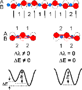
Figure 5-14: Possible types of O jumps between the off-center positions A and B of the zig-zag Cu-O chains.

Also the profile of the potential energy is different in the two cases, since in the first case relaxation occurs between states differing in local strain $2\Delta\lambda$ and in energy by $2\Delta E\neq 0$, while in the second case also the energy must be the same by symmetry (simple inversion of the configuration). Therefore, the origin of the consistent asymmetry $\Delta E/k_{\text{B}}\simeq 210$ K found for peak P4, may be indicative of the energy inequivalence between the two types of chain segments, rather than disorder.

5.5.1 Possible (anti)ferroelastic and (anti)ferroelectric ordering of the off-center oxygen atoms

Finally, we point out that (anti)ferroelastic correlations may arise between the off-centre O atoms, which also involve electric dipoles along the $a$ axis, associated with O^2- atoms that are out-of-axis with respect to the row of Cu²⁺ atoms along $b$. Therefore, such correlations would also be of (anti)ferroelectric nature, although the electric field from these dipoles is effectively screened in the metallic or superconducting environment, and is therefore hardly detectable in experiments. Nonetheless, interactions between neighboring O atoms along the chain or even across adjacent chains cannot be excluded and might even result in short-range (anti)ferroelectric and (anti)ferroelastic domains. Indeed, the $Q^{-1}\left(T\right)$ curves shown here are measured on cooling, but the measurements on heating after some aging below 90 K exhibit clear phase transformations between 120 and 170 K [151], indicated with PT1 and PT2 in Fig. 5-15. In Ref. [151] we discussed how these anomalies in both dissipation and modulus might arise from ferroelectric and/or antiferroelectric domains that are formed during low temperature aging along the Cu-O chains. We also proposed a possible evolution of peak P4 with decreasing $x$ toward a slower and more correlated dynamics, as suggested by a shift to higher temperature and broadening of the peak in some measurements of outgassed samples. Such an increase of the correlation between the chain segments would be due to the decreased electric screening when going into the semiconducting state.

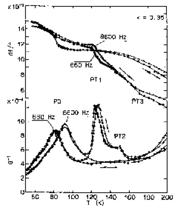
Figure 5-15: Elastic energy loss and resonance frequency ( $\propto\sqrt{E}$) of YBa₂Cu₃O_6.35 measured on cooling and subsequent heating after 20 h at 80 K.

In general, one should be very cautious in considering phase transitions like these, since during several hours of low temperature aging in an ordinary vacuum system without particular precautions a porous sample may adsorb residual gases and then present their solid/liquid transitions on heating. This fact is exemplified by the measurement made on a sample of alumina with $\sim 50\%$ porosity (kindly supplied by E. Roncari at CNR-ISTEC, Faenza, Italy) presented in Fig. 5-16 without using the adsorption pump during the experiment.

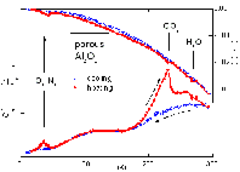
Figure 5-16: Elastic energy loss coefficient and Young’s modulus of porous alumina measured on cooling and subsequent heating. The anomalies on heating correspond the solid/liquid transitions of residual gases adsorbed by the sample.

The measurement on heating present three anomalies around $35-45$ K, 230 K and 268 K, attributable to O₂/N₂, CO₂ and H₂O which were adsorbed onto the porous sample, especially at LHe temperature, and which pass from the solid to the liquid state and finally desorb on heating. It was also possible to monitor an increase of pressure in the system in correspondence with these anomalies. The anomaly of Fig. 5-15, however, should be intrinsic of YBCO, since it occurs at a temperature where nothing is observed in the alumina dummy sample.

5.6 Bipolaron reorientation in the overdoped state

The anelastic relaxation process with the lowest activation energy, $E=0.11$ eV, is labelled P1 and is observed only in the overdoped state: it is absent with $x<0.85$ and its intensity rises very fast on approaching full oxygenation [21]. This is a really noticeable feature, since most of the physical properties of YBCO are practically constant in the range $0.85<x<1$, including the superconducting temperature $T_{\mathrm{C}}\left(x\right)$, which presents a maximum at the so-called optimal doping $x\simeq 0.93$, but whose variation remains within 4% in that range, as shown in Fig. 5-18 from Ref. [152].

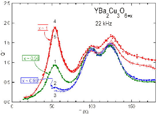
Figure 5-17: Anelastic spectrum of YBa₂Cu₃O_6+x at various values of $x$ in the overdoped region, with peaks P1, P3 and P4, starting from low temperature.

Figure 5-17 presents the anelastic spectrum of YBCO below 180 K, measured at 22 kHz on the same sample in several different states from optimally doped to overdoped, obtained in different ways over a period of 6 years. The peaks at 100 K and 120 K (P3 and P4 discussed above) remain remarkably stable, and only the intensity of P1 at 50 K changes by at least one order of magnitude. Curve 1 is the as-prepared state, where $x$ was estimated from the lattice parameters as $x_{1}\simeq 0.93$ [21]. The curve is closely similar to that measured on an identical sample 6 years earlier and therefore demonstrates the stability of samples and anelastic spectra. Notice that, in view of the near constancy of the lattice parameters for $x>0.9$, the above estimate of $x$ has great uncertainty, and should be increased. In fact, after a mild annealing at 470 K for 20 h in a vacuum better than $10^{-5}$ mbar, some oxygen loss certainly occurred, and $T_{\mathrm{C}}$ increased from 90.3 K to 91.9 K, indicating that the sample passed from the overdoped to the optimally doped state.

With the help of the $T_{\mathrm{C}}\left(x\right)$ curve from literature [152], we can set $x_{1}=0.96$ and $x_{2}=0.93$, as shown in Fig. 5-18. After such a small decrease of the oxygen content, the intensity of P1 decreased by 3-4 times (curve 2); after 15 days the intensity was further reduced (curve 3), possibly due to some oxygen reordering. The sample was then oxygenated as fully as possible in the UHV system described in Sec. 3.5, by heating to 600 ^oC, introducing a static atmosphere of 1250 mbar O₂ and slowly cooling to room temperature (where the O₂ pressure became 740 mbar); the cooling rate was 0.2 K/min except between 490 and 300 ^oC, where it was reduced to 0.1 K/min. After this full oxygenation the intensity of P1 become about twice the original one (curve 4), and remained stable during subsequent runs (curve 5). The sample has been finally outgassed in the UHV system and equilibrated at 460 ^oC with a known amount of O₂, resulting in a final pressure of 9.6 torr O₂, which should result in $x=0.85$ according to the phase diagram of Ref. [153]. From the amount of gas absorbed it was estimated $x=0.89\pm 0.04$, and therefore it can be set $x_{6}=0.87$; at this oxygen content no trace of peak P1 was present.

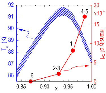
Figure 5-18: Maximum of $T_{\mathrm{C}}\left(x\right)$ inYBa₂Cu₃O_6+x (after [152]). Superimposed in red are the intensities of peak P1 corresponding to the curves in Fig. 5-17 at values of $x$ estimated with the help of the $T_{\mathrm{C}}\left(x\right)$ curve.

Considering that all the structural parameters remain practically constant within the range of $x$ in which P1 develops, it is impossible to associate its mechanism with structural defects, impurities, defects in the order of the Cu-O chains, or off-center atoms, as also discussed in detail in [21]. The only quantity that to our knowledge starts increasing in the same doping range is the concentration of holes of character $p_{z}$, deduced from the peaks in the X-ray absorption spectra (XAS) of the Cu-K edge [115], and shown in Fig. 5-19.

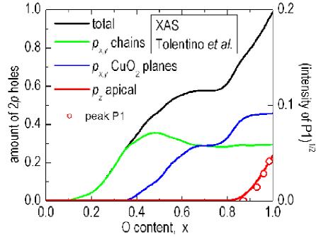
Figure 5-19: Concentration of holes with prevalent O $2p$ character, measured by XAS (from [115]). The concentration of $p_{z}$ holes is evidenced in red, and is in good agreement with $\sqrt{Q_{max}^{-1}}$ of peak P1 (right ordinate axis).

These holes, having symmetry $p_{z}$, must reside on the apical O atoms (see Fig. 5-1), which are the only atoms with consistent hybridization of the $2p_{z}$ orbitals. The correspondence between the growth of the concentration of these holes for $x>0.8$ and the growth of peak P1 is demonstrated in Fig. 5-19, where $\sqrt{Q_{\text{max}}^{-1}}$ of P1 is also plotted. In Fig. 5-20 the $p_{z}$ orbitals are sketched together with those of O $2p_{x}$ and O $2p_{y}$ character, hybridized with the Cu $3d$ orbitals in the CuO₂ planes. Regarding the possible anelastic relaxation processes arising from hopping of the holes among these orbitals, the hopping between $p_{x}$ and $p_{y}$ would of course produce anelastic relaxation, but these holes are extremely mobile, in a band giving rise to superconductivity. The relaxation rate $\tau^{-1}$ characterizing the equilibrium between the $p_{x}$ and $p_{y}$ populations is certainly much faster than the thermally activated rate over a barrier of 0.11 eV found for peak P1. Also the process of change of a hole from $p_{x/y}$ in the CuO₂ plane to apical $p_{z}$ can hardly explain peak P1, since, as already discussed for peak P2 in Sec. 5.4.7, different electronic states are expected to differ in energy in the order of 0.1 eV or more; this would lead to a depression of the relaxation strength by a factor $\cosh^{2}\left(\Delta E/2k_{\text{B}}T\right)$ which, already for $\Delta E=0.1$ eV would be $3\times 10^{-9}$. This means that the relaxation process corresponding to the $p_{x/y}\leftrightarrow p_{z}$ exchange is unobservable.

The hopping of a hole among the $p_{z}$ orbitals of different apical O atoms might well have a correlation time like that of P1, since these orbitals are too much separated to form a band, and two intermediate $p_{x/y}\leftrightarrow p_{z}$ exchanges are necessary. In this case initial and final energy are the same and there is no problem of depression of the relaxation strength; rather, anelastic relaxation is impossible because of the equivalence of all the $p_{z}$ orbitals also under the application of any stress. On the other hand, if two holes on neighboring apical O atoms form a stable pair, a bipolaron, the resulting elastic dipole has orthorhombic symmetry and reorients itself together with the hole pair. It is therefore proposed that peak P1 is due to the reorientation of pairs of holes, or small bipolarons, on neighboring apical O atoms.

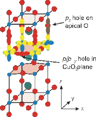
Figure 5-20: $p_{x}$ hole in the CuO₂ plane and $p_{z}$ hole on an apical O in YBa₂Cu₃O${}_{7}.$

The intensity of P1 is then expected to be proportional to the square of the concentration of $p_{z}$ holes, and this is verified in Fig. 5-19, where the square root of the intensity of P1 (closed circles and right ordinate) corresponds very well with the number of $p_{z}$ holes. The activation energy of 0.11 eV would be connected wit the $p_{x/y}\leftrightarrow p_{z}$ exchange process, necessary for the bipolaron reorientation.

It is noticeable that the position in temperature and shape of peak P1 do not change with doping within experimental error. Figure 5-21 presents the experimental data of Fig 5-17 after subtraction of a linear background and normalization to the peak intensity, and all data fall on the same curves. As an additional check of the reliability of the background subtraction, also the difference between curves 4 and 2 is found to fall on the same curves, and it does not depend on the choice of the background.

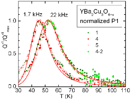
Figure 5-21: Peak P1 after linear background subtraction and normalization to the peak intensity; the symbols are the same of Fig. 5-17 . The continuous line is the fit as explained in text.

The continuous lines are a fit with the Jonscher expression, eq. (2.49), with $\tau_{1}=\tau_{2}=$ $\tau_{0}\exp\left(E/k_{\text{B}}T\right)$ , $\tau_{0}=5\times 10^{-13}$ s, $E/k_{\text{B}}=945$ K, $\alpha=0.33$ and $\beta=0.41$. The values of $\alpha$ and $\beta$ are definitely smaller than 1, indicating considerable broadening with respect to the monodispersive Debye case. This fact is not unexpected, especially for a low-temperature relaxation process in a rather complex and disordered system like YBCO, where random energy shifts due to interaction with various defects, including disorder in the Cu-O chains, may easily be of the order of $0.1-0.2$ times the activation energy. In the present case, however, the main source of disorder are O vacancies in the Cu-O chains, and their concentration $1-x$ decreases of about 4 times from curve 1 to curve 4 without resulting in any narrowing of the peak. Neither can the dynamic interaction among the $p_{z}$ holes be the source of broadening, since also their concentration changes by more than 4 times. The spectrum of relaxation times should therefore be ascribed to the interaction with phonons and the other charge carriers, which remain practically constant within the range $0.85<x<1$ (see also Fig. 5-19).

5.7 The anomaly near 240 K

In YBCO there is a relaxation peak in the absorption around 240 K with the characteristics of glassy dynamics, accompanied by a hysteresis in the Young’s modulus below the same temperature [154, 155, 156]. This anomaly can easily be masked by the freezing transition at $\sim 220$ K of the pump oils adsorbed in porous samples from the measurement vacuum system, as first noticed by Gzowski [31]; in addition, the hysteresis in the elastic moduli may be affected by the sample microstructure [157, 158], since the anisotropic thermal expansion may cause severe stresses from grain to grain during thermal cycling. Nonetheless, an intrinsic effect exists, has a strong dependence on the oxygen content, and has been confirmed by several later works. Regarding the possible mechanism, there are different proposals, like an oxygen ordering transition [154, 155, 133], a ferroelectric or ferromagnetic transition [159] or some polaronic mechanism [160, 161].

5.8 Anomalies at the superconducting temperature

There are various reports of elastic anomalies at the superconducting transition [162, 163, 164], also by means of non traditional techniques [165] and we also found that sometimes anomalies in the Young’s modulus appear near $T_{\text{c}}$. I will not try to analyze such anomalies, considered the multitude of effects affecting the elastic moduli of ceramic samples (see also the previous Section), and, as observed by Mizubayashi et al. [166], the presence of the modulus defects associated with peaks P3 and P4 in the same temperature range (see Fig. 5-12).

5.9 Summary of the main results obtained in YBCO

The interpretation of the anelastic spectra of YBCO starts from the realization that they must be dominated by the hopping with consequent reorientation of the anisotropic elastic dipole of a concentration $0<x<1$ of nonstoichiometric O atoms in the CuO_x planes. One can convince himself or herself of this fact, by noting that in LSCO a concentration $\delta<0.01$ of interstitial O atoms dominates the $Q^{-1}\left(T\right)$ curves (Fig. 4-11b), even though these hopping defects are in a first approximation isotropic (in a tetragonal cell). The barrier for the jumps of O in the CuO_x planes of YBCO has been determined as $\sim 1$ eV from several anelastic relaxation and other types of experiments, but the inspection of spectra at $x\sim 0.1$, 0.4 and 0.9 (Fig. 5-4b) demonstrates that the situation is actually more complex. The complexity should arise from the fact that when an O atom jumps into or out of a chain, not only causes a reorientation of its elastic dipole, but also a change of the electronic energy, possibly by tenths of eV, as discussed in Sec. 5.4.7.

5.9.1 Peak PH2

The peak that is observed at the highest values of $x$ is obviously due to hopping of O atoms in the O-I phase, where the O atoms are ordered into parallel chains. From the $Q^{-1}\left(T\right)$ curves presented here it is impossible to extract any quantitative information, due to the loss of oxygen during the measurements in vacuum, and therefore I accept the picture based on low frequency anelastic experiments [124] that oxygen hopping requires the presence of a vacancy in the neighboring chain. In Sec. 5.4.7, however, it is pointed out that the existing analyses overlook the change in electronic energy that occurs when an O atom leaves or joins a chain; this fact might drastically reduce the number of jumps that actually contribute to the dynamic compliance (due to the depopulation factor Eq. (2.15)) to only those that leave the electronic energy almost unchanged, like the jumps occurring in the twin walls (Fig. 5-10).

5.9.2 Peak PH1

Also in a broad range $0.3<x<0.8$ there is a peak with an activation energy $\sim 1$ eV, but its temperature is definitively lower than that of PH2, and it is labeled here as PH1 (Fig. 4-11b and 5-7a); the fact that PH1 and PH2 are actually distinct peaks is reliability confirmed by low frequency isothermal measurements [140]. The difference between PH1 and PH2 apparently resides in the fact that the latter occurs in an environment of full Cu-O chains, while PH1 might involve all the other jumps, as depicted in Fig. 5-4a (save the possible condition that only jumps of the type of Fig. 5-10 are observable).

5.9.3 Peak P2

The unexpected consequence of reducing $x$ below $0.3$ is that peak PH1 disappears in favor of peak P2 at much lower temperature (Fig. 4-11b and 5-8). This is the only relaxation process that may be assigned to the hopping of isolated O atoms in the CuO_x plane; in fact, quenching experiments exclude that PH1 may contain contributions from isolated O atoms (Fig. 5-7b). Considering that hopping of isolated O atoms must produce a $Q^{-1}\left(T\right)$ well visible down to concentrations well below 0.01, it must be concluded that this peak is P2, with an activation energy of only 0.11 eV. To my knowledge, this is the lowest barrier for oxygen hopping ever reported, comparable to that for hopping of interstitial H in metals. The main difference between jumps of isolated O atoms and those causing peaks PH1 and PH2 is that the latter involve changes in the chemical or electronic state, as discussed in Sec. 5.4.7.

In Sec. 5.4.8 it is also discussed how the unscreened electrostatic repulsion between O atoms in the oxygen-poor semiconducting phase should prevent isolated O atoms to form pairs or join existing chain fragments, so explaining why a small but finite concentration of isolated O atoms survives at the low temperature where peak P2 is observed (otherwise the free O atoms would immediately aggregate into the energetically favorable chains). This also explains the long times (years) necessary for oxygen to reach an equilibrium configuration at room temperature.

5.9.4 Peak P4

At relatively high oxygen contents three $Q^{-1}\left(T\right)$ peaks are observed, with activation energies of $0.08-0.21$ eV (Fig. 5-12). Of these, peak P4 presents a doping dependence compatible with a process occurring in the O-I phase, and it has therefore been associated with short jumps of the O atoms between the sites of the Cu-O chains, which have been shown to be off-centre with respect to the chain axis by diffraction experiments [148, 149].

5.9.5 Peak P1

The evolution of peak P1 with doping, instead, is very peculiar (Figs. 5-17 and 5-18); in fact, it appears only for $x\gtrsim 0.87$ and then grows more than linearly with $x$ in a doping region where virtually all the physical properties, including the superconducting critical temperature, remain almost constant. The only physical quantity that has been reported to display a similar doping dependence is the amount of holes in the $p_{z}$ orbitals of the apical O atoms [115]. Such orbitals have negligible overlap with each other, so that the $p_{z}$ holes cannot form a band but have to pass to orbitals in the CuO₂ planes or CuO_x chains in order to move; this process may well require an activation energy like that of P1, 0.08 eV, and therefore the mechanism proposed for P1 is the reorientation of pairs of $p_{z}$ holes (bipolarons); in fact, the motion of single holes, having the same symmetry of the lattice, would not cause any anelastic relaxation. A confirmation that pairs of $p_{z}$ holes are involved is the proportionality of the intensity of P1 to the square of the concentration of these holes (Fig. 5-19).

Chapter 6 Ru-1212

6.1 Structure

The ruthenocuprates are a relatively new class of HTS,[167] which has attracted much interest for the apparent coexistence of ferromagnetism and superconductivity [168]. RuSr₂GdCu₂O₈ (Ru-1212) has a cell similar to that of YBCO, with Gd instead of Y, SrO instead of BaO layers, and RuO₂ instead of CuO_x planes. Figure 6-1 puts in evidence the CuO₅ pyramids, found also in YBCO, and RuO₆ octahedra, absent in YBa₂Cu₃O_6+x where at most CuO₄ squares in the $bc$ planes exist in correspondence with the chains. From the structural analogy with YBCO, if O vacancies may be introduced in Ru-1212, they are expected to be in the RuO₂ planes. The RuO₆ octahedra are slightly rotated about the $c$ axis in an antiferrodistortive pattern (see Sec. 6.2.1 below), and the rotation angles decreases from 14.4^o at $T=0$ K to 13.9^o at room temperature [169]; a transformation to the symmetric unrotated structure is expected at higher temperature, but not yet observed.

Figure 6-1: Structure of Ru-1212 with the RuO₆ and CuO₅ polyhedra put in evidence.

Doping in Ru-1212 is supposed to be due to the mixed valence of Ru^4+/5+, which, from X-ray absorption spectroscopy [170] and bond valence sums [171], is found to be $40-50\%$ Ru⁴⁺ and the remaining fraction Ru⁵⁺. The mixed valence of Ru is reflected in mixed valence of Cu, with each Ru⁴⁺ considered to inject a hole in one of the CuO₂ planes above or below therefore providing the holes in the usual superconducting CuO₂ planes. However, the deduced concentration of holes $p=$ $\frac{1}{2}\left[\text{Ru}^{4+}\right]=$ $0.2-0.25$ in the CuO₂ planes contrasts with the transport properties, which are typical of underdoped cuprates, therefore with $p\simeq 0.1$. A possible explanation for this incongruence is that most of the holes are trapped by defects or by magnetic order and do not contribute to conductivity [170]. Of course, the presence of O vacancies would affect the charge balance and doping, and therefore also in Ru-1212, as in the other cuprates, it is of general interest to study their formation, dynamics and possible ordering.

In spite of extensive experimental investigations, nominally identical samples may be superconducting or nonsuperconducting, and there is no consensus yet, about the influence of the oxygen stoichiometry and sample microstructure. Some studies find that annealing at high temperature in vacuum or inert atmosphere causes considerable oxygen deficiency [167, 172] while others find no influence at all [173, 169] even up to 800 ^oC [174]. It has then proposed that the prolonged annealings affect the cation ordering [175], the grain boundaries [176], or the microstructure [177].

The $c$ lattice parameter is almost perfectly 3 times greater than $a$, so that there is little mismatch between domains oriented perpendicularly with each other; as a consequence, there is little driving force for the domain growth, and the domain size is very small, unless prolonged aging is made. For this reason, it has been proposed that the reason why superconductivity often presents character of granularity is the high number boundaries where the CuO₂ planes meet at an angle of 90^o; prolonged anneals therefore would favor superconductivity due to the growth of these microdomains and consequent reduction of granularity, rather than stoichiometry changes [170].

Although interesting effects are found also in the anelastic spectrum of Ru-1212 below room temperature [97], in the present Thesis only the high temperature [178] results will be considered.

6.2 Oxygen vacancies

Figure 6-2 presents a series of measurements in vacuum on a same sample at heating/cooling rates of $1.5-3$ K/min, reaching increasing maximum temperatures. The elastic energy loss coefficient $Q^{-1}$ is shown in the lower part, while the upper part is the change of the Young’s modulus relative to the initial value at $T=0$ K. A dissipation peak starts developing above 600 K, and it is due to O vacancies (V${}_{\text{O}}$); in fact, the oxygen loss when heating above that temperature was confirmed by the increase of the oxygen partial pressure during heating ramps in the UHV system. The peak, which is centered at 690 K at 860 Hz and we label as P1, is completely developed after heating up to 850 K and remains stable during further heating/cooling runs up to 930 K. The $Q^{-1}\left(T\right)$ and $E\left(T\right)$ curves measured concomitantly at 9.8 kHz (not shown in the figure) where shifted to higher temperature, indicating that the peak is thermally activated, as expected from jumps of V${}_{\text{O}}$. The relatively fast achievement of an equilibrium spectrum with an intense thermally activated peak, without all the complex phenomenology found in YBCO, indicates that only a small concentration $\delta$ of V${}_{\text{O}}$ can be introduced in RuSr₂GdCu₂O_8-δ, in accordance with other results in the literature. The oxygen loss estimated from the mass loss or gain of a sample subjected to outgassing or oxygenation in the UHV system is $\delta\sim 0.02-0.03$.

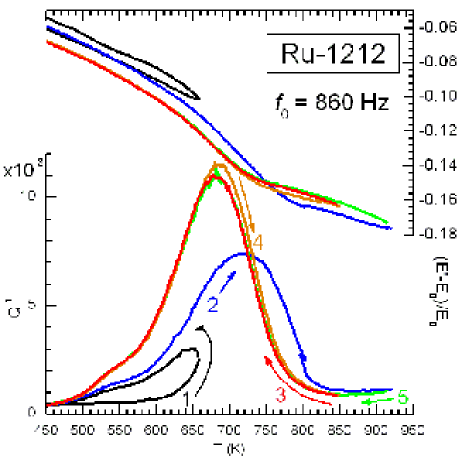
Figure 6-2: Evolution of the anelastic spectrum of Ru-1212 measured in vacuum at progressively higher temperatures.

Since the final spectrum (curves 3 to 5) is stable, it is meaningful to analyze it to make deductions on the dynamics of the O vacancies. In addition, in view of the good quality of the data and rather high values of $Q^{-1}$, instead of $Q^{-1}\left(\omega_{i},T\right)$ I chose to fit the imaginary part of the compliance $s^{\prime\prime}$ referred to the value $s_{0}$ extrapolated to $T=0$ K (the low temperature measurements are not reported here):

$$\frac{s^{\prime\prime}\left[\omega_{i}\left(T\right),T\right]}{s_{0}}=Q^{-1}\left[\omega_{i}\left(T\right),T\right]\,\frac{s^{\prime}\left[\omega_{i}\left(T\right),T\right]}{s_{0}}=Q^{-1}\left[\omega_{i}\left(T\right),T\right]\,\left[\frac{\omega_{i}\left(0\right)}{\omega_{i}\left(T\right)}\right]^{2}$$ (6.1)

so avoiding any approximation of $Q^{-1}\ll 1$; I also took into account the variation of the resonance frequencies $\omega_{i}\left(T\right)$ by 6% and therefore $s^{\prime}$ by 12% within the broad temperature range spanned by the peak. In fact, formulas like eq. (2.50) are valid for both $s^{\prime\prime}$ and $s^{\prime}$ due to the relaxing defect, whereas $s^{\prime}$ generally contains an important temperature dependent contribution $s_{\text{el}}^{\prime}$ from the elastic constants. The resulting $s^{\prime\prime}$ curves are plotted in Fig. 6-3 for both the 1st and 5th vibration modes. There are in fact two peaks: the main one, P1, at 680 K and a smaller one, P2, at 550 K at 0.8 kHz. Figure 6-3a presents a fit with two peaks of the Cole-Cole type, eq. (2.45). It is apparent that such a model of relaxation is inadequate for reproducing the main peak; in fact, i) the intensity of the main peak decreases faster than $1/T$; ii) the parameters for the relaxation time are $\tau_{0}=2.7\times 10^{-18}$ s and $E/k_{\text{B}}=21800$ K; iii) even with these unphysical values of $\tau_{0}$ and $E$ it is impossible to reproduce the asymmetrical broadening of the peak. All these features indicate an anomalous enhancement of both compliance and relaxation time on cooling, as expected from interacting O vacancies in the Curie-Weiss-like approach of Sec. 2.4.

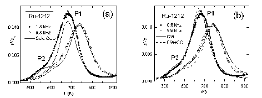
Figure 6-3: Imaginary part of the compliance of Ru-1212 after stabilization of the two peaks. The continuous lines are fits with Cole-Cole peaks (a) and including the Curie-Weiss corrections (b).

Therefore, the fitting function is (see Eq. (2.50))

$$s^{\prime\prime}\left(\omega,T\right) =\Delta\tilde{s}\frac{\omega\tilde{\tau}}{1+\left(\omega\tilde{\tau}\right)^{2}}$$ (6.2)

$$\Delta\tilde{s} =\frac{\Delta s}{T-T_{\mathrm{C}}},\quad\tilde{\tau}=\frac{\tau_{0}\exp\left(E/k_{\text{B}}T\right)}{1-T_{\mathrm{C}}/T}$$ (6.3)

for P1 and again the Cole-Cole formula (2.45) for P2. The resulting fit is the dashed curve in Fig. 6-3b, with the following parameters: $\tau_{0}=1\times 10^{-13}~{}$s, $E=1.33~{}$eV, $T_{\mathrm{C}}=460$ K for P1 and $\tau_{0}=2\times 10^{-17}$ s, $E=1.4$ eV, $\alpha=0.63$ for P2. The fit to P1 is definitely better, even without any broadening parameter, and with a perfectly reasonable value of $\tau_{0}$; this demonstrates that a mean-field scheme of interaction between the V${}_{\text{O}}$ elastic dipoles is able to reproduce the salient properties of P1.

In order to further improve the agreement with the experiment, I introduced a peak broadening according to the Cole-Cole expression, obtaining the continuous lines with the parameters $\tau_{0}=1.1\times 10^{-15}~{}$s, $E=1.46~{}$eV, $T_{\mathrm{C}}=470$ K, $\alpha=0.82$ for P1 and $\tau_{0}=2\times 10^{-14}$ s, $E=1.1$ eV, $\alpha=0.7$ for P2. This broadening is not excessive and may be justified by the high density of boundaries between the three possible orientations of the $c$ axis (see Sec. 6.1) and of antiphase boundaries between domains with opposite directions of the rotation angle of the octahedra about the $c$ axis; the parameters of P1, including the onset temperature $T_{\mathrm{C}}$ of orientational ordering of the elastic dipoles are little affected, but those of P2 assume more physical values. The fact that the fit is not perfect may be ascribed to an inadequacy of the description of the dipole interaction in the mean-field approximation, but also to a variation of the various physical parameters in the broad temperature range from 500 to 900 K. A slow variation in the electronic and/or structural parameters may result in a temperature dependent activation energy $E$. For example, the rotation angle of the RuO₆ octahedra is a linearly decreasing function of temperature within the $0-300$ K range [169] and probably continues decreasing also above room temperature, certainly affecting the hopping parameters of the O vacancies. Incidentally, one might expect a structural transformation to non-rotated octahedra above room temperature, similarly to the case of LSCO and many perovskites, but the anelastic spectra do not show any trace of such a transformation up to 920 K.

Regarding the minor peak P2, no clear indication of $T_{\mathrm{C}}>0$ can be found, also due to the fact that the peak hardly emerges from the tail of P1, but it must also be related with V${}_{\text{O}}$. Two possible origins of P2 are: i) the presence of V${}_{\text{O}}$ also in the CuO₂ planes, although with a much smaller concentration than in the RuO₂ ones; ii) V${}_{\text{O}}$ trapped by some defect in the RuO₂ planes, like Cu substituting Ru.

6.2.1 Rotations of the RuO₆ octahedra

The fact that the RuO₆ octahedra are rotated about the $c$ axes (by about 14${}^{\text{o}}$ at room temperature) complicates only slightly the treatment of the anelasticity due to oxygen hopping within the RuO₂ planes. Figure 6-4a shows the case of non-rotated octahedra, and the $x$ and $y$ axes are chosen parallel to the Ru-O bonds (at 45^o with the standard setting of the $a$ and $b$ cell parameters). The elastic dipoles $\lambda$ associated with V${}_{\text{O}}$ will therefore have major and minor axes parallel to $x$ or $y$; the ellipsoids represent the principal values of $\lambda$ at two O vacancies, compared with the unit circles of no strain at regular O sites (the deviation from unity is exaggerated, and actually an anisotropic expansion instead of contraction might occur, as shown for YBCO in Sec. 5.4.2). Figure 6-4b includes the rotations of the octahedra, again exaggerated, and it can be seen that the strain ellipsoids at the O vacancies remain oriented along $x$ or $y$, which are still symmetry planes of the structure. In conclusion, it is possible to neglect the rotation of the octahedra in analyzing the anelasticity from the hopping of O vacancies.

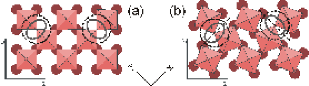
Figure 6-4: RuO₆ octahedra and elastic dipoles (ellipsoids) of two O vacancies neglecting (a) and considerin the rotations of the octahedra about the $c$ axis (b). The dashed unit circles represent the absence of strain.

One might ask why collective dynamic rotations of the octahedra of the type observed in La₂CuO₄ are not found in Ru-1212, even though it has planes of octahedra able to rotate without constraints from outside the plane. The reason is that soliton-like rotation waves cannot develop for rotations about the $c$ axis of octahedra coupled in the $ab$ plane; in fact, it is not possible to decouple rotations along different rows as for the LTT pattern of La₂CuO₄ and therefore it is not possible to derive a one-dimensional equation of motion with solitonic solutions. This can be readily checked in Fig. 6-4, where it appears that the rotation of a single octahedron determines the rotations of all the octahedra in the same plane.

6.2.2 Elastic dipole of the oxygen vacancy and comparison with YBCO

In view of the low concentration $\delta$ of V${}_{\text{O}}$ in the RuO_2-δ planes, it is natural to think in terms of relaxation of V${}_{\text{O}}$ possessing an elastic dipole $\lambda^{\text{V}}$, instead of jumps of O atoms with elastic dipole $\lambda^{\text{O}}$, but the two treatments are otherwise equivalent, with $\lambda^{\text{O}}=-\lambda^{\text{V}}$. This is apparent, for example, also from the symmetry in $c$ and $1-c$ in the equations describing the relaxation of interacting dipoles in Sec. 2.4, where $c=\frac{\delta}{2}$ for RuO_2-δ or $c=\frac{x}{2}$ for CuO_x. From the intensity of peak P1 and the estimated concentration $\delta=0.02-0.03$ of V${}_{\text{O}}$ one can evaluate the anisotropic part $\left|\lambda_{2}-\lambda_{1}\right|$of the elastic dipole of V${}_{\text{O}}$. The estimate is very rough, due to the polycrystalline and highly porous ($\sim 50\%$) nature of the samples. As already done in Sec. 5.4.2 and shown in detail in Appendix B, neglecting porosity (which is of the order of 50% in the present samples), the relaxation strength for V${}_{\text{O}}$ hopping is

$$\Delta=\frac{1}{15}\frac{cv_{0}}{k_{\text{B}}\left(T-T_{\mathrm{C}}\right)\,\left\langle E^{-1}\right\rangle}\left(\Delta\lambda\right)^{2}\,\,,$$ (6.4)

where the Curie-Weiss correction has been included. The Young’s modulus of our sample deduced from Eq. (3.2) was $E=40$ GPa, probably due to the large porosity. Inserting $v_{0}=170\times 10^{-24}$ cm³, $c=0.025$, $T_{\mathrm{C}}=470$ K, $\Delta=$ $2Q_{\text{max}}^{-1}$ $=0.025$ at 680 K one obtains $\Delta\lambda\sim 0.4$; the error in this estimate is large, due to sample porosity and to uncertainties in the determination of $c$, but is about 20 times larger than the value estimated in Sec. 5.4.2 for YBCO from the lattice parameters. A possible justification for the large difference is that the assumption that $\lambda^{\text{O}}=-\lambda^{\text{V}}$ would be valid in the absence of electronic effects, which instead are important.

6.2.3 Possible roles of the oxygen vacancies in determining the superconducting properties

The samples used in the present investigation had been annealed for 1 week at 1070 ^oC in flowing O₂, in order to achieve superconductivity, but no treatments at high O₂ pressure were done. Still, the superconducting transition was in two steps: a first step at 45 K, indicative of intragrain superconductivity, and a second one at 19 K, when the supercurrents flow also between different grains. In these conditions, the anelastic spectrum above room temperature is flat until the oxygen loss starts above 600 K; looking at the $Q^{-1}\left(T\right)$ curve 1 just below 600 K it appears that the initial concentration of O vacancies is at least one order of magnitude smaller than after outgassing, i.e. RuSr₂GdCu₂O_8-δ with $\delta<0.002$. This means that even without high pressure oxygenation the concentration of O vacancies in Ru-1212 is very small, and, also after outgassing, it does not exceed $\delta\sim 0.02-0.03$ (see Sec. 6.2). These values of $\delta$ cannot account for the deficit of conducting holes with respect to the concentration of Ru⁴⁺ ions, as discussed in Sec. 6.2, and therefore the present study supports the view [170] that the scarce reproducibility of the superconducting properties from sample to sample are due to the microstructure rather than to oxygen stoichiometry.

Chapter 7 Conclusions

The main findings described in the present Thesis from the analysis of a large number of anelastic spectra of HTS cuprates can be divided into three types: i) information on the diffusive motion of nonstoichiometric oxygen and its ordering; ii) local and collective motion of oxygen between off-center positions; iii) low frequency fluctuations of the hole stripes pinned by the dopants.

7.0.1 Oxygen diffusion

The most relevant results on the oxygen mobility have been obtained in YBa₂Cu₃O_6+x, where stoichiometry and ordering of oxygen play a fundamental role in determining hole doping. It has been demonstrated that, although it is generally considered that there is a barrier of $\sim 1$ eV for oxygen hopping in the CuO_x planes, there are actually three distinct types of jumps: in the almost fully oxygenated O-I phase, possibly requiring the presence of an O vacancy in the otherwise filled Cu-O chains; jumps involving more sparse Cu-O chain fragments; jumps of isolated O atoms in the semiconducting state over a barrier of only 0.11 eV. The latter process implies an extraordinarily high mobility of the O^2- ions in the nearly empty CuO_x planes, but is not easily identifiable with other experimental techniques, since the O atoms have a strong tendency to form chains, and their concentration as isolated ions is very small already at room temperature. A discussion of the apparent paradoxes posed by such a short hopping time ($10^{-11}$ s at room temperature) and the long characteristic times for reordering (years) has been provided, based on the hypothesis that the electrostatic repulsion between O^2- ions is scarcely screened in the semiconducting states, and rises the barrier for oxygen clustering. An analysis of the oxygen jumps involving changes in the electronic state, also due to charge transfer between Cu-O chains and CuO₂ planes, demonstrates that the situation is more complex than generally supposed in other anelastic spectroscopy studies.

The ruthenocuprate RuSr₂GdCu₂O₈ is isostructural with YBa₂Cu₃O_6+x, except for having RuO_2-δ planes completely filled with oxygen, instead of the CuO_x chains at most half-filled, and it is of interest to ascertain whether the O vacancies are responsible for the difficulty in obtaining reproducible superconducting states. The high temperature anelastic spectra of RuSr₂GdCu₂O_8-δ show that their concentration remains low even after long annealings in vacuum. It is also shown that the O vacancies jump over a barrier of 1.4 eV, create an anisotropic distortion (elastic dipole) much larger than that of oxygen in the CuO_x planes of YBCO, and it is possible to describe the high-temperature anelastic spectrum of Ru-1212 taking into account the long range elastic interaction among these elastic dipoles.

In La_2-xSr_xCuO₄ it is possible to introduce excess oxygen in interstitial positions between layers of CuO₆ octahedra. It has been shown that, although in the ideal tetragonal structure oxygen jumps between these interstitial positions do not cause reorientation of the elastic dipole, this occurs in the slightly distorted orthorhombic structure, and the elastic energy loss peaks associated with jumps of isolated and paired interstitial O atoms have been identified. The formation of stable pairs confirms the existence of peroxyde species lowering the hole transfer to the conducting CuO₂ planes, but it is also shown that such pairs form at much lower concentrations than formerly believed.

7.0.2 Off-centre positions and tilts of the octahedra

In addition to the diffusive motion of nonstoichiometric oxygen, the anelastic spectra demonstrate that oxygen may perform smaller jumps between off-center positions both in YBCO and LSCO. In the first case, an anelastic relaxation process has been identified with the hopping of oxygen between off-center positions on either side of the Cu-O chains (the zig-zag nature of the chains is suggested by diffraction experiments showing anomalously high oxygen thermal factors); it is also suggested that an ordering transition of the chain O atoms in (anti)ferroelastic and (anti)ferroelectric fashion might be responsible for anomalies observed between 120 and 170 K on heating.

In LSCO off-center hopping is connected with the unstable tilts of the oxygen octahedra, responsible for the structural transformations; the anelastic spectra presented here demonstrate that at temperatures much lower than that of the tetragonal-to-orthorhombic transformation and where also the twin motion is frozen, the dynamic modulus (1 kHz) of stoichiometric and defect-free La₂CuO₄ presents still two hardenings of $\sim 25\%$ on cooling below 150 K and of 10% below 10 K; these magnitudes are huge, if one considers that they are not associated to any structural transformation. The first is thermally activated and has been identified as tilt waves of solitonic type within the planes of octahedra, while the second has been identified as faster and local motion of single octahedra or O atoms, with the dynamics determined by quantum tunneling. The fact that octahedral tilts are involved has also been confirmed by NQR measurements, but a consistent picture of these lattice motions has been possible thanks to a complete analysis of the effect of doping through excess oxygen and substitutional Sr. It has therefore been possible to clearly distinguish between collective and local motion and to determine that the local tunneling is strongly coupled to hole excitations, with as little as 3% doping making its dynamics so fast to bring the maximum of the relaxation process below 1 K for frequencies of kHz. This finding suggests that at higher doping the anharmonic potential for the O atoms might be of the type that has been proposed to enhance the electron-phonon coupling to levels necessary for explaining the high-$T_{\mathrm{c}}$ superconductivity [100]. It has also been shown that the spectrum of the hole excitations responsible for the tilt-hole coupling is different from the known cases of electron-lattice interaction governing atomic tunnel systems in other metals or superconductors.

7.0.3 Hole stripes and antiferromagnetic clusters

It has been a surprise to discover that the anelastic spectra of La_2-xSr_xCuO₄ contain clear signatures of the freezing of the Cu²⁺ spins into the cluster spin glass state at $T_{g}\left(x\right)$: a steep rise of the acoustic absorption at $T_{g}$. This absorption has been interpreted in terms of stress induced motion of the walls between the antiferromagnetic clusters with uncorrelated directions of the staggered magnetization, and presenting an anisotropic strain thanks to magnetoelastic coupling. A neutron scattering study [55] is also confirmed, where, at variance with the prevalent opinion, it is proposed that an electronic phase separation occurs for $x<0.02$, with cluster spin glass domains coexisting with long range antiferromagnetic order.

The interest in this finding is enhanced by the fact that, according to the prevalent interpretation, these domain walls coincide with the hole stripes, whose role in high-$T_{\text{c}}$ superconductivity is much discussed, and whose fluctuation dynamics has not been probed by other experiments. Carrying on the analogy between the hole stripes interacting with the Sr²⁺ dopants and other linear defect pinned by impurities, a relaxation process around 80 K at 1 kHz has been identified as due to stripes overcoming the collective pinning barrier by thermal activation, with the measured barrier in very good agreement with a theoretical estimate [60]. The assignment of such a relaxation process to the depinning stripe mechanism has been done after the analysis of a large number of anelastic spectra with Sr doping ranging from $x=0.008$ to 0.20. In this manner, it has also been possible to evidence the effect of stripe-lattice coupling through the tilts of the octahedra, with clear changes when the prevalent stripe orientation passes from parallel to diagonal with respect to the lattice modulation, and near the doping $x=\frac{1}{8}$, where the stripe spacing becomes commensurate with the lattice modulation. The locking of the stripes with domains of low-temperature tetragonal phase near $x=\frac{1}{8}$ has also been seen as a strong depression of the absorption in the cluster spin glass phase in samples containing Ba instead of Sr, due to the reduction of the fraction of mobile stripes. I would like to point out that such phenomena are hardly detectable by other spectroscopies, which are dominated by the response of single charges and spins (dielectric and magnetic susceptibilities, NMR, $\mu$SR) or may probe much shorter characteristic times (light and neutron spectroscopies). The anelastic spectroscopy is instead insensitive to individual charge and spin excitations, and probes only those that are coupled to strain.

Even though it is commonly believed that anelastic experiments are too much affected by grain boundaries, ”defects” and other vagaries, to be able to detect more fundamental excitations or processes, they are as reliable as any other spectroscopy, and the anelastic spectra are perfectly repeatable after years if the samples are good. I hope I showed that anelastic spectroscopy is able to provide reliable and often unique information not only on diffusive, reorientational and tunneling atomic motions, including collective modes like tilts of oxygen octahedra, but also on elusive charge and spin structures like the hole stripes in high-$T_{\text{c}}$ cuprates.

Chapter 8 Appendices

8.1 Appendix A - analytical approximation of the order parameter in the Bragg-Williams model of the CuO_x planes

It is convenient to introduce the order parameter $\xi$, such that

$$c_{1,2}=\frac{c}{2}\left(1\pm\xi\right)$$ (8.1)

with $\xi=0$ and 1 in the completely disordered and ordered states, respectively. Equation (2.65) becomes

$$\ln\left(\frac{\left(1+\xi\right)\left(2-c+c\xi\right)}{\left(1-\xi\right)\left(2-c-c\xi\right)}\right)=\frac{\alpha c}{k_{\text{B}}T}\xi=\frac{4}{\left(2-c\right)}\frac{T_{\mathrm{C}}}{T}\xi$$ (8.2)

A solution $\xi\neq 0$ is possible when the slope of the logarithm in the left hand at small $\xi$, $\frac{4}{2-c}$, is larger than the slope of the linear term, $\frac{\alpha c}{k_{\text{B}}T}$, in the right hand equation; and this determines the critical temperature

$$k_{\text{B}}T_{\mathrm{C}}=\alpha\frac{c}{2}\left(1-\frac{c}{2}\right)\;$$ (8.3)

Figure 8-1 shows the order parameter $\xi\left(t\right)$, solution of eq. (8.2) computed with Mathematica, versus the reduced temperature $t=T/T_{\mathrm{C}}$ for some values of the concentration of dipoles $c$. For $t>0.2$, the $\xi\left(t\right)$ curves become steeper with $c$ increasing up to 0.7, and then acquire again a shape similar to the low-$c$ case. Note that for the case of oxygen in the CuO_x planes of YBCO, there are two oxygen sites per Cu atom, so that in principle $0<x<2$ and the concentration has to be defined as $c=\frac{x}{2}$; however, without doping in the Y or Ba sublattices, it is $0<x<1$, or $c\leq 0.5$. Instead, the RuO_x planes of Ru-1212 have $c\simeq 1$.

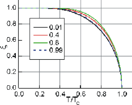
Figure 8-1: Order parameter vs reduced temperature for various concentrations.

The limit $t\rightarrow 0$ or $\xi\rightarrow 1$ can be solved analytically by setting $\xi=1-y$ and obtaining, to first order in $y$,

$$\ln\left(\frac{2}{y\left(1-c\right)}\right)\simeq\frac{4}{\left(2-c\right)t}\rightarrow y=\frac{2}{\left(1-c\right)}\exp\left(-\frac{4}{\left(2-c\right)t}\right)$$ (8.4)

For fitting purposes, it is convenient to have an analytical approximation to $\xi\left(c,t\right)$. A tractable expression, valid for $0<c<0.8$ and $\xi>10^{-2}$, is the following:

$$\xi\left(c,t\right)=\left(1-t^{n}\right)^{m}$$ (8.5)

with $n$ and $m$ depending on concentration as (see also Fig. 8-2)

$$n =3.153+1.785c-2.681c^{2}+9.312c^{3}-8.293c^{4}$$ (8.6)

$$m =0.51+0.02c$$ (8.7)

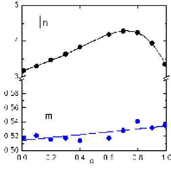
Figure 8-2: Values of the $m$ and $n$ parameters in eq. (8.5) for fitting $\xi\left(c,t\right)$.

For the case $c>0.8$, relevant for Ru-1212, a simple expression like (8.5) is inadequate, but luckily the anelastic relaxation due to oxygen hopping in Ru-1212 at frequencies above $10^{2}$ Hz is well above $T_{\mathrm{C}}$ and there is no need of computing $\xi\left(c,t\right)$.

8.2 Appendix B - relaxation strength in a tetragonal polycrystal

The Young’s modulus of a tetragonal crystal along the direction $\mathbf{\hat{n}}$ is (see e.g. [12])

$$E^{-1}\left(\mathbf{\hat{n}}\right) =S_{11}\left(n_{1}^{4}+n_{2}^{4}\right)+S_{33}n_{3}^{4}+\left(S_{44}+2S_{13}\right)\left(n_{1}^{2}+n_{2}^{2}\right)n_{3}^{2}+$$ (8.8)

$$+\left(S_{66}+2S_{12}\right)n_{1}^{2}n_{2}^{2}+2S_{16}n_{1}n_{2}\left(n_{1}^{2}-n_{2}^{2}\right)$$

where $S_{16}=0$ for various classes, including $4/mmm$, which is appropriate for Ru-1212 [169] and tetragonal YBCO; in this case eq. (8.8) coincides with eq. (6.2-3) of [8] and eq. (A5) of [180]. The O atom or equivalently the O vacancy in the CuO_x or RuO_2-δ planes can be considered as a $\left\langle 100\right\rangle$ orthorhombic defect, which causes relaxation of the elastic constant [180, 8]

$$\delta\left(S_{11}-S_{12}\right)=\frac{cv_{0}}{kT}\frac{1}{2}\left(\lambda_{1}-\lambda_{2}\right)^{2}\,=\delta S^{B_{1}}.$$ (8.9)

Adopting the group theoretical compliances of a tetragonal crystal from Eq. (3.5), p. 125 and Table 5 of [180], the elastic strain $\varepsilon_{i}=s_{ij}\sigma_{j}$ in matrix form may be written as

$$\quad\quad\,\,\,\,\,\,\,\,\,\,\,\,\,\,\,\begin{array}[c]{cccccc}A_{1},1&A_{2},2&B_{1}&B_{2}&E&E\end{array}$$ (8.11)

$$\begin{array}[c]{c}A_{1},1\\ A_{2},2\\ B_{1}\\ B_{2}\\ E\\ E\end{array}\left[\begin{array}[c]{cccccc}s_{33}&\sqrt{2}s_{13}&0&0&0&0\\ \sqrt{2}s_{13}&s_{11}+s_{12}&0&0&0&0\\ 0&0&s_{11}-s_{12}&0&0&0\\ 0&0&0&\frac{1}{2}s_{66}&0&0\\ 0&0&0&0&\frac{1}{2}s_{66}&0\\ 0&0&0&0&0&\frac{1}{2}s_{66}\end{array}\right]\left[\begin{array}[c]{c}\sigma_{3}\\ \frac{1}{\sqrt{2}}\left(\sigma_{1}+\sigma_{2}\right)\\ \frac{1}{\sqrt{2}}\left(\sigma_{1}-\sigma_{2}\right)\\ \sigma_{6}\\ \sigma_{4}\\ \sigma_{5}\end{array}\right]$$ (8.30)

In terms of these compliances eq. (8.8) can be written as

$$E^{-1}\left(\mathbf{\hat{n}}\right) =\overset{S_{11}}{\overbrace{\frac{1}{2}\left(S^{A,22}+S^{B_{1}}\right)}}\left(n_{1}^{4}+n_{2}^{4}\right)+\overset{S_{33}}{\overbrace{S^{A,11}}}n_{3}^{4}+\overset{S_{44}+2S_{13}}{\overbrace{\left(\sqrt{2}S^{A,12}+2S^{E}\right)}}\left(n_{1}^{2}+n_{2}^{2}\right)n_{3}^{2}+$$

$$+\,\overset{S_{66}+2S_{12}}{\overbrace{\left(S^{A,22}+2S^{B_{2}}-S^{B_{1}}\right)}}n_{1}^{2}n_{2}^{2}$$ (8.31)

In the hypothesis that stress is uniform over the polycrystalline sample (Reuss approximation), in order obtain the average $\left\langle\,E^{-1}\right\rangle$ one has to average eq. (8.31) over the angles, with $\left\langle\,n_{i}^{4}\right\rangle=\frac{1}{5}$, $\left\langle n_{i}^{2}n_{j}^{2}\right\rangle=\frac{1}{15}$:

$$\left\langle E^{-1}\right\rangle =\frac{1}{5}S^{A,11}+\frac{4}{15}S^{A,22}+\frac{2\sqrt{2}}{15}S^{A,12}+\frac{2}{15}S^{B_{1}}+\frac{2}{15}S^{B_{2}}+\frac{4}{15}S^{E}=$$ (8.32)

$$=\frac{1}{5}\left(2S_{11}+S_{33}\right)+\frac{1}{15}\left(2S_{44}+S_{66}+4S_{13}+2S_{12}\right)$$

The relaxation of the compliance due to jumps of the orthorhombic defect comes only from $\delta S^{B_{1}}\neq 0$ and therefore

$$\delta\left\langle E^{-1}\right\rangle=\frac{2}{15}\delta S^{B_{1}}=\frac{2}{15}\delta\left(S_{11}-S_{12}\right)$$ (8.33)

and the relaxation strength is

$$\Delta=\frac{\delta\left\langle E^{-1}\right\rangle}{\left\langle E^{-1}\right\rangle}=\frac{2}{15}\frac{\delta\left(S_{11}-S_{12}\right)}{\left\langle E^{-1}\right\rangle}=\frac{1}{15}\frac{cv_{0}}{k_{\text{B}}T\,\left\langle E^{-1}\right\rangle}\left(\lambda_{1}-\lambda_{2}\right)^{2}$$ (8.34)

Porosity strongly affects the elastic moduli [164] and also the relaxation strength in a non-trivial manner, and I simply propose the naive argument that a fraction $p$ of void due to porosity should decrease both $E$ and $\delta E^{-1}$ by $1-p$ (neglecting the effects of the shape of the pores on $E$); therefore it should be

$$\Delta=\frac{\left(\delta E^{-1}\right)_{\text{eff}}}{\left(E^{-1}\right)_{\text{eff}}}=\left(1-p\right)^{2}\frac{\delta E^{-1}}{E^{-1}}\,.$$ (8.35)

List of acronyms and symbols

Acronyms

AF = antiferromagnetic

CSG = Cluster Spin Glass

DW = Domain Wall

EXAFS = Extended X-ray Absorption Fine Structure

HTS = high-temperature superconductor/superconductivity

HTT = High-Temperature Tetragonal

LBCO = La_2-xBa_xCuO₄

LSCO = La_2-xSr_xCuO₄

LTO = Low-Temperature Orthorhombic

LTT = Low-Temperature Tetragonal

$\mu$SR = muon spin relaxation

NCO = Nd₂CuO_4+δ

NMR = Nuclear Magnetic Relaxation

NQR = Nuclear Quadrupolar Relaxation

Ru-1212 = RuSr₂GdCu₂O₈

SG = Spin Glass

TS = Tunnel System

YBCO = YBa₂Cu₃O_6+x

Symbols

$c=$ molar concentration

$c_{ij}=$ elastic stiffness (matrix notation)

$\Delta=$ relaxation strength

$\Delta E=$ energy difference between two states in a relaxation process

$E=$ Young’s modulus, activation energy

$E_{p}=$ pinning barrier for the stripes

$\varepsilon_{ij}=$ strain tensor ($\varepsilon_{i}$ in matrix notation)

$J=$ spectral density (Eq. (2.36))

$L_{c}=$ collective pinning length of the stripes

$\lambda_{ij}=$ elastic dipole tensor ($\lambda_{i}$ in matrix notation)

O = oxygen

O${}_{\text{i}}=$ interstitial O atom

$p=$ hole density

$Q^{-1}=\frac{s^{\prime\prime}}{s^{\prime}}=\frac{c^{\prime\prime}}{c^{\prime}}=$ elastic energy loss coefficient

$s_{ij}=$ elastic compliance (matrix notation)

$\sigma_{ij}=$ stress tensor ($\sigma_{i}$ in matrix notation)

$\tau=$ relaxation time

$T_{\text{c}}=$ superconducting temperature

$T_{\mathrm{C}}=$ Curie-Weiss-like ordering temperature

$T_{d}$ $=$ temperature of the LTO/LTT transition

$T_{g}=$ temperature for freezing into the CSG phase

$T_{\text{N}}=$ Néel temperature for long range AF ordering

$T_{t}$ $=$ temperature of the HTT/LTO transition

V${}_{\text{O}}=$ oxygen vacancy

Bibliography

- [1] D. Larbalestier, A. Gurevich, D.M. Feldmann and A. Polyanskii, Nature 414, 368 (2001).
- [2] S.A.Kivelson, I.P.Bindloss, E.Fradkin, V.Oganesyan, J.M.Tranquada, A. Kapitulnik and C. Howald, Rev. Mod. Phys. 75, 1201 (2003).
- [3] T.M. Rice, Physica C 282-287, xix (1997).
- [4] A. Bianconi, N.L. Saini, T. Rossetti, A. Lanzara, A. Perali, M. Missori, H. Oyanagi, H. Yamaguchi, Y. Nishihara and D.H. Ha, Phys. Rev. B 54, 12018 (1996).
- [5] S.A. Kivelson, E. Fradkin and V.J. Emery, Nature 393, 550 (1998).
- [6] J. Zaanen, Nature 404, 714 (2000).
- [7] C. Zener, Elasticity and Anelasticity of Metals. (Univ. of Chicago Press, Chicago, 1948).
- [8] A.S. Nowick and B.S. Berry, Anelastic Relaxation in Crystalline Solids. (Academic Press, New York, 1972).
- [9] A.T. Savici, Y. Fudamoto, I.M. Gat, T. Ito, M.I. Larkin, Y.J. Uemura, G.M. Luke, K.M. Kojima, Y.S. Lee, M.A. Kastner, R.J. Birgeneau and K. Yamada, Mechanical Spectroscopy Q-1 2001: with Applications to Materials Science. ed. by R. Schaller, G. Fantozzi and G. Gremaud, (Trans Tech Publications, Totton, UK, 2001).
- [10] J.F. Nye, Physical Properties of Crystals; their Representation by Tensors and Matrices. (Oxford University Press, Oxford, UK, 1957).
- [11] G. Leibfried and N. Breuer, Point Defects in Metals I. (Springer, Berlin, 1978).
- [12] Yu.I. Sirotin and M.P. Shaskolskaya, Fundamentals of crystal physics. (Mir Publishers, Moscow, 1982).
- [13] F. Cordero, Phys. Rev. B 47, 7674 (1993). In this paper there are some errors without consequences on any of the conclusions: Eq. (4) should be and the line below ””; in Eqs. (9, 11, 19, 20, 30, 39, 40, 48, 49, 62) must be substituted with or with .
- [14] H. Wipf and K. Neumaier, Phys. Rev. Lett. 52, 1308 (1984).
- [15] L.D. Landau and E.M. Lifshitz, Statistical Physics. (Pergamon, London, 1959).
- [16] H. Wipf and B. Kappesser, J. Phys.: Condens. Matter 8, 7233 (1996).
- [17] A. Rigamonti, F. Borsa and P. Carretta, Rep. Prog. Phys. 61, 1367 (1998).
- [18] S. Kamba, V. Bovtun, J. Petzelt, I. Rychetsky, R. Mizaras, A. Brilingas, J. Banys, J. Grigas and M. Kosec, J. Phys.: Condens. Matter 12, 497 (2000).
- [19] F. Cordero, M. Corti, F. Craciun, C. Galassi, D. Piazza and F. Tabak, Phys. Rev. B 71, 94112 (2005).
- [20] R.M. Fuoss and J.G. Kirkwood, J. Am. Chem. Soc. 63, 385 (1941).
- [21] G. Cannelli, R. Cantelli, F. Cordero, F. Trequattrini and M. Ferretti, Phys. Rev. B 54, 15537 (1996).
- [22] A.K. Jonscher, Nature 256, 673 (1975).
- [23] D. de Fontaine, G. Ceder and M. Asta, Nature 343, 544 (1990).
- [24] M. Ausloos and A. Pekalski, Phys. Rev. B 52, 4577 (1995).
- [25] K. Skwarek, A. Pekalski and M. Ausloos, Eur. Phys. J. B 11, 369 (1999).
- [26] F. Brenscheidt, D. Seidel and H. Wipf, J. Alloys and Compounds 211/212, 264 (1994).
- [27] S. Dattagupta, J. Phys. F: Metal Phys. 12, 1363 (1982).
- [28] S. Dattagupta, R. Balakrishnan and R. Ranganathan, J. Phys. F: Met. Phys. 12, 1345 (1982).
- [29] G. Haneczok, M. Weller and J. Diehl, phys. stat. sol. (b) 172, 557 (1992).
- [30] C. Artini, M.M. Carnasciali, G.A. Costa, M. Ferretti, M.R. Cimberle, M. Putti and R. Masini, Physica C 377, 431 (2002).
- [31] B. Kusz, M. Gazda, O. Gzowski, I. Davoli and S. Stizza, IV National Conference on High Transition Temperature Superconductivity - SATT4, Parma, Italy, 13 (1991).
- [32] S. Braccini, C. Casciano, F. Cordero, F. Corvasce, M. De Sanctis, R. Franco, F. Frasconi, E. Majorana, G. Paparo, R. Passaquieti, P. Rapagnani, F. Ricci, D. Righetti, A. Solina and R. Valentini, Meas. Sci. Technol. 11, 467 (2000).
- [33] F. Cordero, R. Cantelli and M. Ferretti, J. Appl. Phys. 92, 7206 (2002).
- [34] F. Cordero and R. Cantelli, Physica C 312, 213 (1999).
- [35] F.C. Chou, J.H. Cho and D.C. Johnston, Physica C 197, 303 (1992).
- [36] P.G. Radaelli, J.D. Jorgensen, A.J. Schultz, B.A. Hunter, J.L. Wagner, F.C. Chou and D.C. Johnston, Phys. Rev. B 48, 499 (1993).
- [37] J.-S. Zhou, H. Chen and J.B. Goodenough, Phys. Rev. B 50, 4168 (1994).
- [38] E.S. Bozin, S.J.L. Billinge, G.H. Kwei and H. Takagi, Phys. Rev. B 59, 4445 (1999).
- [39] C. Rial, E. Moràn, M.A. Alario-Franco, U. Amador and N.H. Andersen, Physica C 254, 233 (1995).
- [40] J.D. Axe, A.H. Moudden, D. Hohlwein, D.E. Cox, K.M. Mohanty, A.R. Moodenbaugh and Y. Xu, Phys. Rev. Lett. 62, 2751 (1989).
- [41] M.K. Crawford, R.L. Harlow, E.M. McCarron, W.E. Farneth, J.D. Axe, H. Chou and Q. Huang, Phys. Rev. B 44, 7749 (1991).
- [42] W.E. Pickett, R.E. Cohen and H. Krakauer, Phys. Rev. Lett. 67, 228 (1991).
- [43] M. Nohara, T. Suzuki, Y. Maeno, T. Fujita, I. Tanaka and H. Kojima, Phys. Rev. Lett. 70, 3447 (1993).
- [44] Y. Koyama, Y. Wakabayashi, K. Ito and Y. Inoue, Phys. Rev. B 51, 9045 (1995).
- [45] A.R. Moodenbaugh, L. Wu, Y. Zhu, L.H. Lewis and D.E. Cox, Phys. Rev. B 58, 9549 (1998).
- [46] E. Takayama-Muromachi and D.E. Rice, Physica C 177, 195 (1991).
- [47] T. Fukase, T. Nomoto, T. Hanaguri, T. Goto and Y. Koike, Physica B 165/6, 1289 (1990).
- [48] A. Bussmann-Holder, A. Migliori, Z. Fisk, J.L. Sarrao, R.G. Leisure and S.-W. Cheong, Phys. Rev. Lett. 67, 512 (1991).
- [49] H. Takagi, T. Ido, S. Ishibashi, M. Uota, S. Uchida and Y. Tokura, Phys. Rev. B 40, 2254 (1989).
- [50] F.C. Chou, F. Borsa, J.H. Cho, D.C. Johnston, A. Lascialfari, D.R. Torgeson and J. Ziolo, Phys. Rev. Lett. 71, 2323 (1993).
- [51] E. Lai and R.J. Gooding, Phys. Rev. B 57, 1498 (1998).
- [52] A.N. Lavrov, Y. Ando, S. Komiya and I. Tsukada, Phys. Rev. Lett. 87, 017007 (2001).
- [53] R.J. Gooding, N.M. Salem, R.J. Birgeneau and F.C. Chou, Phys. Rev. B 55, 6360 (1997).
- [54] Ch. Niedermayer, C. Bernhard, T. Blasius, A. Golnik, A. Moodenbaugh and J.I. Budnick, Phys. Rev. Lett. 80, 3843 (1998).
- [55] M. Matsuda, M. Fujita, K. Yamada, R.J. Birgeneau, Y. Endoh and G. Shirane, Phys. Rev. B 65, 134515 (2002).
- [56] J.M. Tranquada, B.J. Sternlieb, J.D. Axe, Y. Nakamura and S. Uchida, Nature 375, 561 (1995).
- [57] J.M. Tranquada, N. Ichikawa and S. Uchida, Phys. Rev. B 59, 14712 (1999).
- [58] S. Wakimoto, G. Shirane, Y. Endoh, K. Hirota, S. Ueki, K. Yamada, R.J. Birgeneau, M.A. Kastner, Y.S. Lee, P.M. Gehring and S.H. Lee, Phys. Rev. B 60, 769 (1999).
- [59] S. Wakimoto, R.J. Birgeneau, M.A. Kastner, Y.S. Lee, R. Erwin, P.M. Gehring, S.H. Lee, M. Fujita, K. Yamada, Y. Endoh, K. Hirota and G. Shirane, Phys. Rev. B 61, 3699 (2000).
- [60] C. Morais Smith, Yu.A. Dimashko, N. Hasselmann and A.O. Caldeira, Phys. Rev. B 58, 453 (1998).
- [61] F. Cordero, A. Paolone, R. Cantelli and M. Ferretti, Phys. Rev. B 64, 132501 (2001).
- [62] R.S. Markiewicz, F. Cordero, A. Paolone and R. Cantelli, Phys. Rev. B 64, 54409 (2001).
- [63] A. Paolone, F. Cordero, R. Cantelli and M. Ferretti, Phys. Rev. B 66, 94503 (2002).
- [64] A. Paolone, R. Cantelli, F. Cordero, M. Corti, A. Rigamonti and M. Ferretti, Int. J. Mod. Phys. B 17, 512 (2003).
- [65] F. Cordero, A. Paolone, R. Cantelli and M. Ferretti, Phys. Rev. B 67, 104508 (2003).
- [66] J.H. Cho, F.C. Chou and D.C. Johnston, Phys. Rev. Lett. 70, 222 (1993).
- [67] R.S. Markiewicz, J. Phys. Chem. Solids 58, 1179 (1997).
- [68] S.J.L. Billinge and P.M. Duxbury, Phys. Rev. B 66, 64529 (2002).
- [69] K. Yamada, C.H. Lee, Y. Endoh, G. Shirane, R.J. Birgeneau and M.A. Kastner, Physica C 282-287, 85 (1997).
- [70] M. Fujita, K. Yamada, H. Hiraka, P.M. Gehring, S.H. Lee, S. Wakimoto and G. Shirane, Phys. Rev. B 65, 64505 (2002).
- [71] Y. Tokura, H. Takagi and S. Uchida, Nature 337, 345 (1989).
- [72] W.-K. Lee, M. Lew and A.S. Nowick, Phys. Rev. B 41, 149 (1990).
- [73] J.L. Sarrao, D. Mandrus, A. Migliori, Z. Fisk, I. Tanaka, H. Kojima, P.C. Canfield and P.D. Kodali, Phys. Rev. B 50, 13125 (1994).
- [74] D.C. Johnston, Handbook of Magnetic Materials. ed. by K.H.J. Buschow, p. 1 (North Holland, 1997).
- [75] J.C. Phillips and K.M. Rabe, Phys. Rev. B 44, 2863 (1991).
- [76] A.R. Moodenbaugh and D.E. Cox, Physica C 341-348, 1775 (2000).
- [77] P. Blakeslee, R.J. Birgeneau, F.C. Chou, R. Christianson, M.A. Kastner, Y.S. Lee and B.O. Wells, Phys. Rev. B 57, 13915 (1998).
- [78] H.H. Feng, Z.G. Li, P. Hor, S. Bhavaraju, J.F. DiCarlo and A.J. Jacobson, Phys. Rev. B 51, 16499 (1995).
- [79] F. Cordero, C.R. Grandini, G. Cannelli, R. Cantelli, F. Trequattrini and M. Ferretti, Phys. Rev. B 57, 8580 (1998).
- [80] F. Cordero, C.R. Grandini and R. Cantelli, Physica C 305, 251 (1998).
- [81] F.C. Chou and D.C. Johnston, Phys. Rev. B 54, 572 (1996).
- [82] B. Kappesser, H. Wipf and R.K. Kremer, J. Low Temp. Phys. 105, 1481 (1996).
- [83] J.D. Jorgensen, B. Dabrowski, S. Pei, D.R. Richards and D.G. Hinks, Phys. Rev. B 40, 2187 (1989).
- [84] C. Chaillout, S.W. Cheong, Z. Fisk, M.S. Lehmnann, M. Marezio, B. Morosin and J.E. Schirber, Physica C 158, 183 (1989).
- [85] D. Haskel, E.A. Stern, D.G. Hinks, A.W. Mitchell, J.D. Jorgensen and J.I. Budnick, Phys. Rev. Lett. 76, 439 (1996).
- [86] M.K. Crawford, R.L. Harlow, E.M. McCarron, W.E. Farneth, J.D. Axe, H. Chou and Q. Huang, J. Phys. Chem. Solids 56, 1459 (1995).
- [87] C.R. Michel and N. Casan-Pastor, Physica C 278, 149 (1997).
- [88] F. Cordero, M. Corti, M. Campana, A. Rigamonti, R. Cantelli and M. Ferretti, Int. J. Mod. Phys. B 13, 1079 (1999).
- [89] T. Kamiyiama, F. Izumi, H. Asano, H. Takagi, S. Uchida, Y. Tokura, E. Takayama- Muromachi, M. Matsuda, K. Yamada, Y. Endoh and Y. Hidaka, Physica C 172, 120 (1990).
- [90] R.S. Markiewicz, Physica C 210, 264 (1993).
- [91] F. Cordero, R. Cantelli, M. Corti, M. Campana and A. Rigamonti, Phys. Rev. B 59, 12078 (1999).
- [92] S. Aubry, J. Chem. Phys. 62, 3217 (1975).
- [93] S. Torre and A. Rigamonti, Phys. Rev. B 36, 8274 (1987).
- [94] M. Braden, A.H. Moudden, S. Nishizaki, Y. Maeno and T. Fujita, Physica C 273, 248 (1997).
- [95] M. Braden, W. Reichardt, S. Nishizaki, Y. Mori and Y. Maeno, Phys. Rev. B 57, 1236 (1998).
- [96] H. Matsui, M. Yamaguchi, Y. Yoshida, A. Mukai, R. Settai, Y. Onuki, H. Takei and N. Toyota, J. Phys. Soc. Jpn. 67, 3687 (1998).
- [97] A. Paolone, F. Cordero, R. Cantelli, G.A. Costa, C. Artini, A. Vecchione and M. Gombos, J. Magn. Magn. Mater. 272-276, 2106 (2004).
- [98] F. Cordero, R. Cantelli and M. Ferretti, Phys. Rev. B 61, 9775 (2000).
- [99] G. Cannelli, R. Cantelli, F. Cordero and F. Trequattrini, Tunneling Systems in Amorphous and Crystalline Solids. ed. by P. Esquinazi, p. 389 (Springer, Berlin, 1998).
- [100] A. Bussmann-Holder, A.R. Bishop and I. Batistic, Phys. Rev. B 43, 13728 (1991).
- [101] S. Wakimoto, S. Ueki, Y. Endoh and K. Yamada, Phys. Rev. B 62, 3547 (2000).
- [102] M.-H. Julien, A. Campana, A. Rigamonti, P. Carretta, F. Borsa, P. Kuhns, A.P. Reyes, W.G. Moulton, M. Horvatic, C. Berthier, A. Vietkin and A. Revcolevschi, Phys. Rev. B 63, 144508 (2001).
- [103] F. Cordero, A. Paolone, R. Cantelli and M. Ferretti, Phys. Rev. B 62, 5309 (2000).
- [104] N. Hasselmann, A.H. Castro Neto, C. Morais Smith and Y. Dimashko, Phys. Rev. Lett. 82, 2135 (1999).
- [105] S. Bogner and S. Scheidl, Phys. Rev. B 64, 54517 (2001).
- [106] M. Bosch, W. van Saarloos and J. Zaanen, Phys. Rev. B 63, 92501 (2001).
- [107] T. Nattermann, Y. Shapir and I. Vilfan, Phys. Rev.B 42, 8577 (1990).
- [108] J.F. Qu, Y. Liu, F. Wang, X.Q. Xu and X.G. Li, Phys. Rev. B 71, 94503 (2005).
- [109] R. McCormack, D. de Fontaine and G. Ceder, Phys. Rev. B 45, 12976 (1992).
- [110] J.D. Jorgensen, B.W. Veal, A.P. Paulikas, L.J. Nowicki, G.W. Crabtree, H. Claus and W.K. Kwok, Phys. Rev. B 41, 1863 (1990).
- [111] G. Uimin, H. Haugerud and W. Selke, Physica C 275, 93 (1997).
- [112] D. Mønster, P.-A. Lindgård and N.H. Andersen, Phys. Rev. B 64, 224520 (2001).
- [113] H. Lütgemeier, S. Schmenn, P. Meuffels, O. Storz, R. Schöllhorn, Ch. Niedermayer, I. Heinmaa and Yu. Baikov, Physica C 267, 191 (1996).
- [114] J.M. Tranquada, S.M. Heald, A.R. Moodenbaugh and ouwen Xu, Phys. Rev. B 38, 8893 (1988).
- [115] H. Tolentino, F. Baudelet, A. Fontaine, T. Gourieux, G. Krill, J.Y. Henry and J. Rossat-Mignod, Physica C 192, 115 (1992).
- [116] A. Bianconi, A.C. Castellano, M. Desantis, P. Rudolf, P. Lagarde, A.M. Flank and A. Marcelli, Solid State Commun. 63, 1009 (1987).
- [117] P. Schleger, W.N. Hardy and H. Casalta, Phys. Rev. B 49, 514 (1994).
- [118] G. Uimin and J. Rossat-Mignod, Physica C 199, 251 (1992).
- [119] A. Krol, Z.H. Ming, Y.H. Kao and N. N, Phys. Rev. B 45, 2581 (1992).
- [120] K. Conder, Mater. Sci. Engin.: R 32, 41 (2001).
- [121] J.L. Routbort and S.J. Rothman, J. Appl. Phys. 76, 5615 (1994).
- [122] J.R. LaGraff and D.A. Payne, Phys. Rev. B 47, 3380 (1993).
- [123] K.N.Tu,C.C.Tsuei,S.I. Park, and A. Levi, Phys. Rev. B 38, 772 (1988).
- [124] X.M. Xie, T.G. Chen and Z.L. Wu, Phys. Rev. B 40, 4549 (1989).
- [125] J.R. Cost and J.T. Stanley, J. Mater. Res. 6, 232 (1991).
- [126] J. Woirgard, P. Gadaud, A. Riviere and B. Kaya, Mat. Sci. Forum 119-121, 719 (1993).
- [127] F. Brenscheidt, K. Foos and H. Wipf, Europhys. Lett. 39, 275 (1997).
- [128] G. Cannelli, R. Cantelli and F. Cordero, Phys. Rev. B 38, 7200 (1988).
- [129] M. Canali, G. Cannelli, R. Cantelli, F. Cordero, M. Ferretti and F. Trequattrini, Physica C 185-189, 897 (1991).
- [130] G. Cannelli, R. Cantelli, F. Cordero, F. Trequattrini and M. Ferretti, Solid State Commun. 82, 433 (1992).
- [131] G. Cannelli, R. Cantelli, F. Cordero and F. Trequattrini, Supercond. Sci. Tech. 5, 247 (1992).
- [132] H. Casalta, P. Schleger, P. Harris, B. Lebech, N.H. Andersen, R. Liang, P. Dosanjh and W.N. Hardy, Physica C 258, 321 (1996).
- [133] Q. Wang, G.A. Saunders, D.P. Almond, M. Cankurtaran and K.C. Goretta, Phys. Rev. B 52, 3711 (1995).
- [134] Y. Shindo, H. Ledbetter and H. Nozaki, J. Mater. Res. 10, 7 (1995).
- [135] D. Seidel, A. Hornes and H. Wipf, Europhys. Lett. 18, 307 (1992).
- [136] R. Tétot, V. Pagot and C. Picard, Phys. Rev. B 59, 14748 (1999).
- [137] H. Wipf, Solid State Commun. 91, 713 (1994).
- [138] G. Cannelli, R. Cantelli, F. Cordero, F. Trequattrini, S. Ferraro and M. Ferretti, Solid State Commun. 80, 715 (1991).
- [139] J.R. Cost and J.T. Stanley, Scripta metall. mater. 28, 773 (1993).
- [140] Y. Mi, R. Schaller and W. Benoit, J. Alloys Comp. 211/212, 283 (1994).
- [141] R. Bormann and J. Nölting, Appl. Phys. Lett. 54, 2148 (1989).
- [142] G. Cannelli, R. Cantelli, F. Cordero, M. Ferretti and F. Trequattrini, Solid State Commun. 77, 429 (1991).
- [143] G. Jang, C. Bucci, R. De Renzi, G. Guidi, M. Varotto, C. Serge and P. Radaelli, Physica C 226, 301 (1994).
- [144] S. de Brion, J.Y. Henry, R. Calemczuk and E. Bonjour, Europhys. Lett. 12, 281 (1990).
- [145] G. Cannelli, R. Cantelli, F. Cordero, N. Piraccini, F. Trequattrini and M. Ferretti, Phys. Rev. B 50, 16679 (1994).
- [146] B.W. Veal, A.P. Paulikas, H. You, H. Shi, Y. Fang and J.W. Downey, Phys. Rev. B 42, 6305 (1990).
- [147] G. Cannelli, R. Cantelli, F. Cordero, M. Ferretti and L. Verdini, Phys. Rev. B 42, 7925 (1990).
- [148] M. Francois, A. Junod, K. Yvon, A. W. Hewat, J. J. Capponi, P. Strobel, M. Marezio and P. Fischer, Solid State Commun. 66, 1117 (1988).
- [149] W. Wong-Ng, F. W. Gayle, D. L. Kaiser, S. F. Watkins and F. R. Fronczek, Phys. Rev. B 41, 4220 (1990).
- [150] A. Nath and Z. Homonnay, Physica C 161, 205 (1989).
- [151] G. Cannelli, M. Canali, R. Cantelli, F. Cordero, S. Ferraro, M. Ferretti and F. Trequattrini, Phys. Rev. B 45, 931 (1992).
- [152] V. Breit, P. Schweiss, R. Hauff, H. Wühl, H. Claus, H. Rietschel, A. Erb and G. Müller-Vogt, Phys. Rev. B 52, 15727 (1995).
- [153] P. Schleger, W.N. Hardy and B.X. Yang, Physica C 176, 261 (1995).
- [154] G. Cannelli, R. Cantelli, F. Cordero, G.A. Costa, M. Ferretti and G.L. Olcese, Europhys. Lett. 6, 271 (1988).
- [155] T. Laegreid and K. Fossheim, Europhys. Lett. 6, 81 (1988).
- [156] H.M. Ledbetter and S.A. Kim, Phys. Rev. B 38, 11857 (1988).
- [157] S. Ewert, S. Guo, P. Lemmens, F. Stellmach, J. Wynants, G. Arlt, D. Bonnenberg, H. Kliem, A. Comberg and H. Passing, Solid State Commun. 64, 1153 (1987).
- [158] E. Biagi, E. Borchi, R. Garre, S. Degennaro, L. Masi and L. Masotti, phys. stat. sol. (a) 138, 249 (1993).
- [159] L.N. Pal-Val, P.P. Pal-Val, V.D. Natsik and V.I. Dotsenko, Solid State Commun. 81, 761 (1992).
- [160] X.N. Ying and Y.N. Wang, Solid State Commun. 123, 511 (2002).
- [161] X.N. Ying, Y.N. Huang and Y.N. Wang, Supercond. Sci. Technol. 17, 347 (2004).
- [162] T.J. Kim, J. Kowalewski, W. Assmus and W. Grill, Z. Physik B 78, 207 (1990).
- [163] J. Dominec, Supercond. Sci. Technol. 6, 153 (1993).
- [164] H. Ledbetter, M. Lei, A. Hermann and Z. Sheng, Physica C 225, 397 (1994).
- [165] T.J. Kim, E. Mohler and W. Grill, J. Alloys and Compounds 212, 318 (1994).
- [166] H.Mizubayashi,K. Takita, and S. Okuda, Phys. Rev. B 37, 9777 (1988).
- [167] L. Bauernfeind, W. Widder and H.F. Braun, Physica C 254, 151 (1995).
- [168] A. Fainstein, E. Winkler, A. Butera and J. Tallon, Phys. Rev. B 60, R12597 (1999).
- [169] O. Chmaissem, J.D. Jorgensen, H. Shaked, P. Dollar and J.L. Tallon, Phys. Rev. B 61, 6401 (2000).
- [170] A.C. McLaughlin, W. Zhou, J.P. Attfield, A.N. Fitch and J.L. Tallon, Phys. Rev. B 60, 7512 (1999).
- [171] R.S. Liu, L.-Y. Jang, H.-H. Hung and J.L. Tallon, Phys. Rev. B 63, 212507 (2001).
- [172] M. Matvejeff, V.P.S. Awana, L.-Y. Jang, R.S. Liu, H. Yamauchi and M. Karppinen, Physica C 392-396, 87 (2003).
- [173] D.J. Pringle, J.L. Tallon, B.G. Walker and H.J. Trodahl, Phys. Rev. B 59, R11679 (1999).
- [174] R.W. Henn, H. Friedrich, V.P.S. Awana and E. Gmelin, Physica C 341-348, 457 (2000).
- [175] P.W. Klamut, B. Dabrowski, M. Maxwell, J. Mais, O. Chmaissem, R. Kruk, R. Kmiec and C.W. Kimball, Physica C 341-348, 455 (2000).
- [176] B. Lorenz, R.L. Meng, J. Cmaidalka, Y.S. Wang, J. Lenzi, Y.Y. Xue and C.W. Chu, Physica C 363, 251 (2001).
- [177] J.L. Tallon, J.W. Loram, G.V.M. Williams and C. Bernhard, Phys. Rev. B 61, R6471 (2000).
- [178] F. Cordero, M. Ferretti, M.R. Cimberle and R. Masini, Phys. Rev. B 67, 144519 (2003).
- [179] A.W. Hunt, P.M. Singer, K.R. Thurber and T. Imai, Phys. Rev. Lett. 82, 4300 (1999).
- [180] A.S. Nowick and W.R. Heller, Adv. Phys. 14, 101 (1965).