Three–body Correlation Effects on the Spin Dynamics of Double–Exchange Ferromagnets

Abstract

We present a variational calculation of the spin wave excitation spectrum of double–exchange ferromagnets in different dimensions. Our theory recovers the Random Phase approximation and 1/S expansion results as limiting cases and can be used to study the intermediate exchange coupling and electron concentration regime relevant to the manganites. In particular, we treat exactly the long range three–body correlations between a Fermi sea electron–hole pair and a magnon excitation and show that they strongly affect the spin dynamics in the parameter range relevant to experiments in the manganites. The manifestations of these correlations are many-fold. We demonstrate that they significantly change the ferromagnetic phase boundary. In addition to a decrease in the magnon stiffness, we obtain an instability of the ferromagnetic state against spin wave excitations close to the Brillouin zone boundary. Within a range of intermediate concentrations, we find a strong softening of the spin wave dispersion as compared to the Heisenberg ferromagnet with the same stiffness, which changes into hardening for other concentrations. We discuss the relevance of these results to experiments in colossal magnetoresistance ferromagnets.

I Introduction and problem setup

The interactions between itinerant carriers and local magnetic moments lead to new magnetic properties in a wide variety of systems that have been the subject of intense research lately. Examples where such magnetic exchange and Hund’s rule interactions play an imporant role range from ferromagnetic semiconductors such as EuO, EuS, chrome spinels, or pyrochlore nagaev to dilute III-Mn-V and II-VI magnetic semiconductors. III-V-1 ; III-V-2 Of particular interest here are the manganese oxides (manganites) R_1-xA_xMnO₃, where R=La, Pr, Nd, Sm, $\cdots$ and A= Ca, Ba, Sr, Pb, $\cdots$, which display colossal magnetoresistance. tokura ; dagotto The above systems display ferromagnetic order mediated by itinerant carriers. Our main goal in this paper is to describe the role of ubiquitous three–body correlations (beyond the mean field approximation) on the spin dynamics of such ferromagnets.

Given the wide variety of such ferromagnetic systems, it is important to understand the properties of the minimal Hamiltonian that describes the common properties and spin dynamics. In order to calculate the effects of correlations beyond the mean field approximation, it is often necessary to neglect particularities of the individual systems, such as chemical structure and crystal environment. The most basic model that applies to all such materials is the Kondo lattice or double exchange Hamiltonian $H=K+H_{exch}+H_{super}+H_{U}$, where $K=\sum_{{\bf k}\sigma}\varepsilon_{{\bf k}}c^{\dagger}_{{\bf k}\sigma}c_{{\bf k}\sigma}$ is the kinetic energy of the itinerant carriers. In the manganites (R_1-xA_xMnO₃), $n=1-x$ itinerant electrons per Mn atom occupy the band of Mn d–states with e_g symmetry. We simplify the calculation of the three–body correlations of interest here by considering a single tight–binding band of cubic symmetry and neglect the bandstructure and the degeneracy of the e_g states (which may be lifted by external perturbations). The operator $c^{\dagger}_{{\bf k}\sigma}$ creates an electron with momentum ${\bf k}$, spin $\sigma$, and energy $\varepsilon_{{\bf k}}=-2t\sum_{i=1}^{d}\cos k_{i}a$, where $d=1,2,3$ is the system dimensionality and $a$ is the lattice constant. From now on we take $a=1$ and measure the momenta in units of $\hbar/a$.

A common feature of all the systems of interest here is the strong magnetic exchange interaction, $H_{exch}$, between the itinerant carrier spins and the local spin–S magnetic moments ${\bf S}_{i}$, which are located at the $N^{d}$ lattice sites ${\bf R}_{i}$. In the manganites, these S=3/2 spins are due to the three electrons in the tightly bound t_2g orbitals. Introducing the collective localized spin operator ${\bf S}_{{\bf q}}=1/\sqrt{N}\sum_{j}{\bf S}_{j}e^{-i{\bf q}{\bf R}_{j}}$ and the corresponding spin lowering operator $S^{-}_{{\bf q}}=S^{x}_{{\bf q}}-iS^{y}_{{\bf q}}$, we express the local magnetic exchange interaction in momentum space:

$$H_{exch} = -\frac{J}{2\sqrt{N}}\sum_{{\bf k}{\bf q}\sigma}\,\sigma\,S_{{\bf q}}^{z}\ c_{{\bf k}-{\bf q}\sigma}^{\dagger}c_{{\bf k}\sigma}$$ (1)

$$-\frac{J}{2\sqrt{N}}\sum_{{\bf k}{\bf q}}\left(S_{{\bf q}}^{-}\ c_{{\bf k}-{\bf q}\uparrow}^{\dagger}c_{{\bf k}\downarrow}+h.c.\right),$$

where $\sigma=\pm 1$. In the manganites, $J>0$ describes the ferromagnetic Hund’s rule coupling between the local and itinerant spins on each lattice site. $H_{super}$ is the weak antiferromagnetic direct superexchange interaction between the spins localized in neighboring sites, while $H_{U}$ describes the local Coulomb (Hubbard) repulsion among the itinerant electrons. The precise values of the parameters entering in the above Hamiltonian are hard to calculate for strongly coupled many–body systems such as the manganites. Although the parameter estimates vary in the literature, typical values are $t\sim$ 0.2-0.5 eV and $J\sim$ 2eV, which corresponds to $4\leq J/t\leq 10$. dagotto On the other hand, the antiferromagnetic superexchange interaction is weak, $\sim 0.01t$. The electron concentration, $n=(N_{e}/N)^{d}=1-x$ where $N_{e}$ is the number of electrons, varies from 0 to 1. Ferromagnetism in the metallic state is observed within a concentration range $0.5\leq n\leq 0.8$ in both 3D and quasi–2D (layered) systems. In this paper we neglect for simplicity the effects of $H_{super}$ and $H_{U}$ (to be studied elsewhere) in order to focus $H_{exch}$.

Given the large values of $J/t$ in most systems of interest, a widely used approximation is the $J\rightarrow\infty$ limit (double exchange ferromagnet). de In this strong coupling limit, the itinerant carrier is allowed to hop on a site only if its spin is parallel to the local spin on that site. The kinetic energy is then reduced when all itinerant and local spins are parallel, which favors a ferromagnetic ground state (double exchange mechanism). We denote this fully polarized half–metallic state by $|F\rangle$ and note that it is an eigenstate of our Hamiltonian $H$. This state describes local spins with $S_{z}=S$ on all lattice sites and a Fermi sea of spin–$\uparrow$ itinerant electrons occupying all momentum states with $\varepsilon_{{\bf k}}\leq E_{F}$, where $E_{F}$ is the Fermi energy.

Another commonly used approximation is to treat the local spins as classical ($S\rightarrow\infty$ limit). dagotto The ferromagnetism can then be described by an effective nearest neighbor Heisenberg model with ferromagnetic interaction. The quantum effects are often taken into account perturbatively in 1/S. This 1/S expansion can be implemented systematically by using the Holstein–Primakoff bosonization method. golosov ; chubukov ; nagaev To $O(1/S)$, this method gives noninteracting Random Phase Approximation (RPA) magnons, whose dispersion is determined by the exchange interaction. furukawa ; RPA In the strong coupling limit $J/t\rightarrow\infty$, this RPA dispersion coincides with that of the nearest neighbor Heisenberg ferromagnet. The $O(1/S^{2})$ correction to the spin wave dispersion however deviates from this Heisenberg form. This correction comes from the scattering of the RPA magnon with the spin–$\uparrow$ electron Fermi sea when treated to lowest order in the electron–magnon interaction strength (Born approximation). golosov ; chubukov

The role of nonperturbative carrier–magnon correlations (beyond $O(1/S^{2})$) has been studied by exact diagonalization of small and 1D systems num-1 ; num-2 or by using variational wavefunctions okabe ; wurth inspired from the Hubbard model and the Gutzwiller wavefunction. roth ; rucken ; ander ; linden The variational calculations of Refs.okabe, ; wurth, treat the local correlations expected to dominate in the strong coupling limit. rucken The ferromagnetic (Nagaoka) state $|F\rangle$ was shown to become unstable with increasing electron concentration due to the softening of either single particle spin excitations ander or long wavelength spin wave excitations (negative stiffness).okabe ; wurth The spin wave dispersion deviated from the Heisenberg form for very small electron concentrations.wurth In the concentration range $0.5\leq n\leq 0.8$ relevant to the manganites, Wurth et.al. wurth found small deviations from the Heisenberg form. A similar conclusion was reached based on the 1/S expansion.chubukov For $n\sim 0.7$, the $O(1/S^{2})$ magnon dispersion showed a relative hardening at the zone boundary in the strong coupling limit. chubukov Given the questions raised in the literature about the adequacy of the simple double exchange model for explaining the magnetic and transport properties of the manganites dagotto , it is important to treat the Hamiltonian $H$ in a controlled way in the parameter regime relevant to the manganites. Such a treatment would allow us to assess the accuracy of the commonly used approximations and understand the successes and limitations of the very basic model in explaining the experiments.

Due to the interplay between the spin and charge degrees of freedom, a good understanding of the spin dynamics is important for understanding the physics of colossal magnetoresistance and transport in the manganites. Several experimental studies of the spin wave excitation spectrum have been reported in the literature. Heisenberg–like magnons were observed in the ferromagnetic regime for high electron concentrations (typically $n>0.7$). sw-exp-1 This observation is consistent with the spin wave spectrum obtained in the classical spin limit or by using the strong coupling RPA. However, for lower electron concentrations $0.5\leq n\leq 0.7$, unexpectedly strong deviations from the short range Heisenberg magnon dispersion were observed in several different manganites. soft-exp-1 ; soft-exp-2 ; soft-exp-3 ; soft-exp-4 ; endoh ; soft-2D-1 ; soft-2D-2 Most striking is the pronounced softening of the spin wave dispersion and short magnon lifetime close to the zone boundary, which indicate a new spin dynamics in the metallic ferromagnetic phase for intermediate electron concentrations $0.5\leq n\leq 0.7$. The physical origin of this dynamics remains under debate. It has been conjectured that the coupling to additional degrees of freedom not included in the double exchange Hamiltonian $H$ is responsible for this new spin dynamics. Some of the mechanisms that have been proposed involve the orbital degrees of freedom, the spin–lattice interaction, the local Hubbard interaction, bandstructure effects, etc. endoh ; khal ; golosov ; solovyev ; mochena .

In this paper we study variationally the low energy spin excitations of the half–metallic fully polarized state $|F\rangle$. Our focus is on the role of correlations. Our theory treats exactly up to three–body correlations between a magnon and a Fermi sea pair by using the most general variational wavefunction that includes up to one Fermi sea pair excitations. As already noted in the context of the Hubbard model, rucken ; linden the Gutzwiller wavefunction, which treats local correlations, wurth ; okabe is a special case of such a wavefunction. Here we treat both local and long–range correlations on equal footing in momentum space in order to interpolate between the weak and strong coupling limits with the same formalism. We treat nonperturbatively in a variational way the multiple electron–magnon and hole–magnon scattering processes that lead to vertex corrections of the carrier–magnon interaction. The above two scattering channels are coupled by three–body correlations. We show that this coupling is important for the intermediate electron concentrations and exchange interactions relevant to the manganites, while for small (large) $n$ the electron–magnon (hole–magnon) scattering channel dominates. In the case of the 1D Hubbard model, a similar three–body treatment gave excellent agreement with the exact results. igarashi Analogous calculations were performed to describe the electron–Fermi sea pair local Hubbard interactions igarashi ; rucken ; linden and the valence (or core) hole–Fermi sea pair interactions that lead to the Fermi Edge ( X–ray Edge) Singularity. perakis ; ssr

Our variational wavefunction offers several advantages. While local correlations wurth ; okabe dominate in the strong coupling limit, long range correlations become important as $J/t$ decreases.rucken By working in momentum space, we treat both long and short range correlations while addressing both the weak and strong coupling limits with the same formalism. We therefore expect that our results interpolate well for the intermediate values of $J/t$ relevant to the manganites. rucken Our wavefunction satisfies momentum conservation automatically, which reduces the number of independent variational parameters. Furthermore, our results become exact in the two limits of $N_{e}=1$ and $N_{e}=N^{d}$. We therefore expect that they interpolate well for intermediate electron concentrations $0<n<1$. Our variational equations contain the RPA ($O(1/S)$), ladder diagram approximation, and $O(1/S^{2})$ results as special cases. Finally, our results converge with increasing system size $N$ and thus apply to the thermodynamic limit. The only restriction is that we neglect contributions from two or more Fermi sea pair excitations. Such multipair contributions are however suppressed for large $S$, while their contribution in the case of the 1D Hubbard model was shown to be small. igarashi ; ssr

Here we address a number of issues regarding the effects of up to three–body carrier–magnon correlations on the spin dynamics predicted by the simplest double exchange Hamiltonian. First, by comparing to the 1/S expansion, RPA, and ladder approximation results, we show that vertex corrections and long range three–body magnon–Fermi sea pair correlations, which couple the electron–magnon and hole magnon scattering channels, play an important role on the spin dynamics in the parameter regime relevant to the manganites. We find large deviations from the strong coupling double exchange spin wave dispersion, including a strong magnon softening at the zone boundary in the intermediate electron concentration and exchange interaction regime. On the other hand, for small electron concentrations (relevant e.g. in III(Mn)V semiconductors III-V-1 ; III-V-2 ), the electron-magnon multiple scattering processes dominate. However, even in this regime the deviations from the RPA and $O(1/S^{2})$ magnon dispersions can be strong.

Second, by using an unbiased variational wavefunction, we determine the change in the ferromagnetic phase boundary due to the three–body correlations and carrier–magnon vertex corrections (not included to $O(1/S^{2})$). The variational nature of our calculation allows us to rigorously conclude that the ferromagnetic state $|F\rangle$ is unstable when its energy exceeds that of the variational spin wave energy. In addition to the long wavelength softening and eventual instability, which occurs in all dimensions, we find another instability for momenta close to the zone boundary while the stiffness remains positive. This instability only occurs in 2D and 3D for intermediate electron concentrations ($0.4\leq n\leq 0.7$ for the 2D three–body calculation). This effect is exacerbated by the three–body correlations. One should contrast the above instability to the spin wave softening (but not instability) at the zone boundary that occurs for small $n<0.3$.chubukov ; golosov ; wurth

Third, we study the deviations from the Heisenberg spin wave dispersion induced by the three–body correlations and vertex corrections. This comparison is important given the experimental observation of pronounced deviations for $n\leq 0.7$. soft-exp-1 ; soft-exp-2 ; soft-exp-3 ; soft-exp-4 ; endoh ; soft-2D-1 ; soft-2D-2 Deviations from Heisenberg behavior already occur to $O(1/S^{2})$, or even to $O(1/S)$ for finite $J/t$, but in most cases correspond to magnon hardening.chubukov By comparing our results to the Heisenberg dispersion with the same stiffness, we show that, for values of $J/t$ relevant to the manganites and such that the ferromagnetic state is stable up to $n\sim 0.8$ or higher, the three–body correlations in the 2D system give magnon hardening at the zone boundary for $n\leq 0.4$ followed by strong magnon softening for $0.4<n\leq 0.7$ and then small magnon hardening for $n>0.7$. This behavior is similar to the experiment.

The outline of this paper is as follows. In Section II we discuss the four approximations that we use to calculate the effects of the carrier–magnon correlations on the spin wave dispersion. In Section II.A we discuss the variational wavefunction that treats the three–body correlations. The variational equations that determine the spin wave dispersion are presented in Appendix I. We also obtain the RPA magnon dispersion variationally. In Section II.B we establish the connection between the above variational results and the 1/S expansion results. chubukov ; golosov We show, in particular, that the $O(1/S^{2})$ magnon dispersion can be obtained from our variational equations by treating the carrier–magnon scattering to lowest order in the corresponding interaction strength (Born approximation). In Section II.C we discuss the two–body ladder approximation, obtained from our variational results by neglecting the coupling between the electron–magnon and hole–magnon scattering channels. The latter coupling is discussed further in Appendix II. In Section II.D we discuss the approximation of carrier–localized spin scattering and show that this variational treatment improves on the RPA while making the numerical calculation of three–body effects feasible in much larger systems. In Section III we present our numerical results for the spin wave dispersion, ferromagnetic phase diagram, and deviations from Heisenberg dispersion in the 1D, 2D, and 3D systems and compare between the different approximations. We end with the conclusions.

II Calculations

In this section we discuss the four approximations that we use to treat the effects of the carrier–magnon correlations. From now on we measure the energies $\omega_{{\bf Q}}$ of the spin wave states with respect to that of the fully polarized (half–metallic) ferromagnetic state $|F\rangle$, whose stability and low energy spin excitations we wish to study. We note that $|F\rangle$ is an exact eigenstate of the Hamiltonian $H$ with maximum spin value and total spin z–component $N(S+n/2)$. To study the stability of this state in a controlled way, it is important to use approximations that allow us to draw definite conclusions. This is possible with the variational principle, which allows us to conclude that a negative excitation energy $\omega_{{\bf Q}}$ means instability of $|F\rangle$, driven by the spin wave of momentum ${\bf Q}$. Our variational states have the form $|{\bf Q}\rangle=M^{{\dagger}}_{{\bf Q}}|F\rangle$, where the operator $M^{{\dagger}}_{{\bf Q}}$ conserves the total momentum, lowers the z–component of the total spin by 1, and includes up to one Fermi sea pair excitations. A spin wave has total spin z–component of $N(S+n/2)-1$, which corresponds to one reversed spin as compared to $|F\rangle$. This spin reversal can be achieved either by lowering the localized spin z–component by 1 or by coherently promoting an electron from the spin–$\uparrow$ band to the spin–$\downarrow$ band. The spin reversal can be accompanied by the scattering (shakeup) of Fermi sea pairs. From now on we use the indices ${\bf\nu,\mu},\cdots$ to denote single electron states inside the Fermi surface and ${\bf\alpha,\beta},\cdots$ to denote states outside the Fermi surface.

II.1 Three–body Correlations

In this section we discuss our three-body variational calculation of the spin wave dispersion. First, however, we show that the well known RPA magnon dispersion furukawa ; RPA can be obtained variationally for any value of $J/t$ by neglecting in $M^{{\dagger}}_{{\bf Q}}$ all Fermi sea pair excitations. The most general such operator has the form

$$M^{{\dagger}}_{{\bf Q}RPA}=S^{-}_{{\bf Q}}|F\rangle+\frac{1}{\sqrt{N}}\sum_{{\bf\nu}}X_{{\bf\nu}}^{{\bf Q}RPA}c^{\dagger}_{{\bf Q}+{\bf\nu}\downarrow}c_{{\bf\nu}\uparrow},$$ (2)

where the variational equations for the $N_{e}$ amplitudes $X_{{\bf\nu}}^{RPA}$ are obtained in Appendix I (Eq.(13)). In the strong coupling limit $JS\rightarrow\infty$, $X^{RPA}\rightarrow 1$ and $M^{{\dagger}}_{{\bf Q}RPA}$ reduces to the total spin operator. To lowest order in $t/JS$ we obtain from Eqs. (12) and (13) that the RPA dispersion then reduces to the Heisenberg dispersion

$$\omega_{{\bf Q}}^{RPA}=\frac{1}{2N}\frac{1}{S+n/2}\sum_{{\bf\nu}<k_{F}}\left(\varepsilon_{{\bf v\nu}+{\bf Q}}-\varepsilon_{{\bf\nu}}\right)+O(t/JS).$$ (3)

The $O(1/S)$ magnon dispersion chubukov ; furukawa is obtained from the above strong coupling RPA result by replacing the total spin prefactor $S+n/2$ by $S$.

We now include in $M_{{\bf Q}}^{\dagger}$ the most general contribution of the one Fermi sea pair states:

$$M_{{\bf Q}}^{\dagger}=S_{{\bf Q}}^{-}+\frac{1}{\sqrt{N}}\sum_{{\bf\nu}}X_{{\bf\nu}}^{{\bf Q}}\ c_{{\bf Q}+{\bf\nu}\downarrow}^{{\dagger}}c_{{\bf\nu}\uparrow}+\sum_{{\bf\alpha}{\bf\mu}}c_{{\bf\alpha}\uparrow}^{{\dagger}}c_{{\bf\mu}\uparrow}\times$$

$$\left[\Psi^{{\bf Q}}_{{\bf\alpha}{\bf\mu}}\ S_{{\bf Q}+{\bf\mu}-{\bf\alpha}}^{-}\right.+\left.\frac{1}{2\sqrt{N}}\sum_{{\bf\nu}}\Phi^{{\bf Q}}_{\alpha\mu\nu}c_{{\bf Q}+{\bf\mu}-{\bf\alpha}+{\bf\nu}\downarrow}^{{\dagger}}c_{{\bf\nu}\uparrow}\right],$$ (4)

where the amplitudes $X^{{\bf Q}}_{{\bf\nu}},\,\Psi^{{\bf Q}}_{{\bf\alpha\mu}}$ and $\Phi^{{\bf Q}}_{{\bf\alpha\mu\nu}}$ are all determined variationally; we do not use the RPA results for $X^{{\bf Q}}$ and $\Phi^{{\bf Q}}$. As compared to previous calculations, we do not assume any particular form or momentum dependence for the above variational amplitudes. This allows us to treat in an unbiased way the long range correlations for any value of $J/t$. The first two terms on the rhs of Eq.(II.1) create a magnon of momentum ${\bf Q}$. The last two terms describe the scattering of a momentum ${\bf Q}$ magnon to momentum ${\bf Q}+{\bf\nu}-{\bf\alpha}$ with the simultaneous scattering of a Fermi sea electron from momentum ${\bf\mu}<k_{F}$ to momentum ${\bf\alpha}>k_{F}$.

Our wavefunction Eq. (II.1) becomes exact in the two limits of $N_{e}=1$ and $N_{e}=N^{d}$. To see this, we note that, for $N_{e}=1$, the Fermi sea consists of a single electron. As a result, multipair excitations do not contribute, while $\Phi^{{\bf Q}}=0$. In the half–filling limit $N_{e}=N^{d}$, all lattice sites are occupied by one spin–$\uparrow$ electron and the Fermi sea occupies all momentum states up to the zone boundary. As a result, the RPA wavefunction Eq. (2) becomes exact. Eq. (II.1) also gives the exact wavefunction in the atomic limit $t=0$, $\varepsilon_{k}=0$, where the variational amplitudes do not depend on the electron momenta. To see this, we note that, due to the Pauli principle, $\Phi_{{\bf\alpha\mu\nu}}^{{\bf Q}}$ must be antisymmetric with respect to the exchange of the Fermi sea electron momenta $\nu$ and $\mu$. In the atomic limit, $\Phi^{{\bf Q}}$ must therefore vanish since it is independent of the momenta. For the same reason, all multipair amplitudes vanish as well and Eq.(II.1) gives the exact result.

The variational equation for $\Psi^{{\bf Q}}$ is derived in Appendix I (Eqs.(14) and (17)). The magnon energy is obtained from Eq. (10) after substituting Eq. (11):

$$\omega_{{\bf Q}}=\frac{J}{2N}\sum_{{\bf\nu}}\frac{\varepsilon_{{\bf\nu}+{\bf Q}}-\varepsilon_{{\bf\nu}}-\omega_{{\bf Q}}}{JS+\varepsilon_{{\bf\nu}+{\bf Q}}-\varepsilon_{{\bf\nu}}-\omega_{{\bf Q}}}+\sum_{{\bf\nu}}\Gamma^{e}_{{\bf\nu}}.$$ (5)

where we introduced the electron vertex function

$$\Gamma^{e}_{{\bf\nu}}=\frac{J}{2N}\frac{\varepsilon_{{\bf\nu}+{\bf Q}}-\varepsilon_{{\bf\nu}}-\omega_{{\bf Q}}}{JS+\varepsilon_{{\bf\nu}+{\bf Q}}-\varepsilon_{{\bf\nu}}-\omega_{{\bf Q}}}\sum_{{\bf\alpha}^{\prime}}\Psi^{{\bf Q}}_{{\bf\alpha}^{\prime}{\bf\nu}}.$$ (6)

The first term in Eq.(5) gives the RPA contribution to the magnon energy. The second term is the carrier–magnon self energy contribution, determined by the electron vertex function $\Gamma^{e}$. The latter satisfies Eq.(20), which describes the multiple electron–magnon scattering contribution (ladder diagrams, two–body correlations) as well as the coupling to the hole vertex function, Eq. (19), due to the three–body correlations. Below we discuss three contributions to the full $\Gamma^{e}$: $O(1/S^{2})$ (Born scattering approximation), ladder diagram (two–body carrier–magnon correlations), and the contribution due to carrier scattering with the localized spins.

II.2 1/S Expansion

In this section we make the connection with the Holstein–Primakoff bosonization treatment of the quantum effects. golosov ; chubukov In particular, we show that the $O(1/S^{2})$ magnon dispersion golosov ; chubukov can be obtained by solving Eq.(20) perturbatively, to lowest order in the carrier–magnon interaction and 1/S.

First, we recall that classical spin behavior is obtained in the limit $S\rightarrow\infty$ with $JS$=finite. By expanding Eqs (17), (6) and (19) in powers of the small parameter 1/S ($JS$= finite) we see that $\Psi^{{\bf Q}}=O(1/S)$, $\Gamma^{e}=O(1/S^{2})$, and $\Gamma^{h}=O(1/S^{2})$. In particular, we obtain from Eq.(20) to lowest order in 1/S

$$\Gamma^{e}_{{\bf\nu}}=-\frac{J^{2}}{4N^{2}}\left(\frac{\varepsilon_{{\bf\nu}+{\bf Q}}-\varepsilon_{{\bf\nu}}}{JS+\varepsilon_{{\bf\nu}+{\bf Q}}-\varepsilon_{{\bf\nu}}}\right)^{2}\sum_{{\bf\alpha}}\frac{1}{\varepsilon_{{\bf\alpha}}-\varepsilon_{{\bf\nu}}},\ \$$ (7)

and from Eq.(5)

$$\omega_{{\bf Q}} = \frac{J}{2N}\sum_{{\bf\nu}}\frac{\varepsilon_{{\bf\nu}+{\bf Q}}-\varepsilon_{{\bf\nu}}-\omega_{{\bf Q}}}{JS+\varepsilon_{{\bf\nu}+{\bf Q}}-\varepsilon_{{\bf\nu}}-\omega_{{\bf Q}}}$$ (8)

$$-\frac{J^{2}}{4N^{2}}\sum_{{\bf\alpha}{\bf\nu}}\frac{\left(\varepsilon_{{\bf\nu}+{\bf Q}}-\varepsilon_{{\bf\nu}}\right)^{2}}{\left(JS+\varepsilon_{{\bf\nu}+{\bf Q}}-\varepsilon_{{\bf\nu}}\right)^{2}\left(\varepsilon_{{\bf\alpha}}-\varepsilon_{{\bf\nu}}\right)}.\ \$$

The last term in the above equation comes from the lowest order magnon–electron scattering contribution. The $O(1/S)$ spin wave dispersion furukawa is obtained from the first term by neglecting $\omega_{{\bf Q}}=O(1/S)$ in the denominator. The spin wave energy to $O(1/S^{2})$ is obtained by expanding the first term to this order. We recover the strong coupling $O(1/S^{2})$ results of Refs golosov, ; chubukov, , obtained by using the bosonization technique, by further expanding Eq.(8) in the limit $JS\rightarrow\infty$.

The $O(1/S^{2})$ magnon dispersion is not variational. Thus we cannot definetely conclude instability of the ferromagnetic state if we find a negative magnon energy to $O(1/S^{2})$. On the other hand, the three–body calculation outlined in the previous section treats the magnon–Fermi sea pair interaction variationally rather than perturbatively (as in the 1/S expansion) while recovering the $O(1/S^{2})$ results as a special case. The n–pair contributions to Eq.(II.1) have amplitudes of order $O(1/S^{n})$. Therefore, the shake–up of multipair excitations is suppressed for large $S$. Our three–body calculation thus puts the $O(1/S^{2})$ results on a more quantitative (variational) basis by treating fully rather than perturbatively all contributions of the one Fermi sea pair states.

adaa

II.3 Two–body Ladder Approximation

To go beyond the Born approximation ($O(1/S^{2})$), we first consider the two–body correlation contributions to the Fermi sea pair amplitude $\Psi^{{\bf Q}}$ while still neglecting the three–body correlations. This is equivalent to treating the ladder diagrams that describe the multiple electron–magnon and hole–magnon scattering, while neglecting the coupling between these two scattering channels. Noting that the magnon dispersion is determined by $\Gamma^{e}$ only (Eq.(5)), the ladder approximation dispersion is obtained from Eq. (20) with $\Gamma^{h}=0$ and Eq.(5):

$$\omega_{{\bf Q}}=\frac{J}{2N}\sum_{{\bf\nu}}\frac{\varepsilon_{{\bf\nu}+{\bf Q}}-\varepsilon_{{\bf\nu}}-\omega_{{\bf Q}}}{JS+\varepsilon_{{\bf\nu}+{\bf Q}}-\varepsilon_{{\bf\nu}}-\omega_{{\bf Q}}}$$

$$+\frac{J^{2}}{4N^{2}}\sum_{{\bf\nu}}\frac{\left(\frac{\varepsilon_{{\bf\nu}+{\bf Q}}-\varepsilon_{{\bf\nu}}-\omega_{{\bf Q}}}{JS+\varepsilon_{{\bf\nu}+{\bf Q}}-\varepsilon_{{\bf\nu}}-\omega_{{\bf Q}}}\right)^{2}\sum_{{\bf\alpha}^{\prime}}1/\Delta^{{\bf Q}}_{{\bf\alpha}^{\prime}{\bf\nu}}}{1-\frac{J}{2N}\frac{\varepsilon_{{\bf\nu}+{\bf Q}}-\varepsilon_{{\bf\nu}}-\omega_{{\bf Q}}}{JS+\varepsilon_{{\bf\nu}+{\bf Q}}-\varepsilon_{{\bf\nu}}-\omega_{{\bf Q}}}\sum_{{\bf\alpha}^{\prime}}1/\Delta^{{\bf Q}}_{{\bf\alpha}^{\prime}{\bf\nu}}},$$ (9)

where $\Delta^{{\bf Q}}$ is given by Eq.(A). We note that, similar to the 1/S expansion, the above ladder approximation result is not variational. A similar approximation was used in the context of the Fermi Edge Singularity. perakis ; ssr There it was shown that at least three–body correlations are necessary in order to describe the unbinding of the discrete exciton bound state. perakis ; ssr In the case of the Hubbard model, the ladder approximation was shown to overestimate the electron self energy. igarashi

The difference between the spin wave dispersions Eq.(II.3) and the full three–body calculation comes from the three–body correlations. By comparing the corresponding curves in the next section we can therefore judge the role of these correlations on the spin dynamics.

II.4 Carrier–localized spin scattering ($\Phi=0,\Psi\neq 0$)

To describe the three–body correlations, the coupled equations for $\Gamma^{e}$ and $\Gamma^{h}$ must be solved. Although this is possible in 1D and 2D for fairly large systems, in 3D the numerical solution of the full variational equations is challenging, due to the dependence of $\Gamma^{h}_{{\bf\alpha}{\bf\nu}}$ on six momentum components. On the other hand, $\Gamma^{e}_{{\bf\nu}}$ depends on one momentum only. The dependence of $\Gamma^{h}_{{\bf\alpha}{\bf\nu}}$ on the momentum ${\bf\nu}$ can be eliminated by considering a simpler variational wavefunction, obtained from Eq.(II.1) by setting $\Phi=0$. This corresponds to treating fully the scattering of the electron with the localized spins while neglecting the electronic contribution to the scattered magnon. This approximation becomes exact in the two limits $N_{e}=1$ and $N_{e}=N^{d}$ and also recovers the $O(1/S^{2})$ and RPA results. Its main advantage is that it improves the RPA by allowing us to treat variationally three-body carrier–localized spin correlations in a large system. The corresponding spin wave dispersion is obtained by solving the coupled Eqs.(20) and (21) and then substituting $\Gamma^{e}$ in Eq.(5).

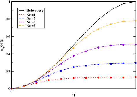
Figure 1: Spin-wave dispersion at the $J\rightarrow\infty$ limit in a 1D system with N =20, S =1/2 and for number of electrons Ne =1, 3, 5, 7. The points in the figure show exact results.

III Numerical results

In this section we present the results of our numerical calculations. First of all, we compare our numerical results with results made by exact diagonalization of small 1D systemnum-1 ; num-2 . Fig 1 shows the comparison where we see that our results are in very good agreement with the exact calculations. To draw conclusions on the role of the correlations, we compare the different approximations discussed in the previous section for a d–dimensional lattice with $N^{d}$ sites. We perform our calculations for d=1, 2, and 3. The dimensionality of the system affects the quantum fluctuations and correlation effects. Quantum fluctuations are expected to be most pronounced in the 1D system, where we show that the 1/S expansion can lead to spurious features. The calculation of the 1D magnon dispersion could also be relevant to quasi–1D materials with chain structures. Our 2D magnon dispersion is relevant to the quasi–2D layered manganites, magnon-2D ; 2D-mang where a pronounced spin wave softening and deviations from the Heisenberg dispersion similar to the 3D system soft-exp-1 ; soft-exp-2 ; soft-exp-3 ; soft-exp-4 ; endoh were observed experimentally. soft-2D-1 ; soft-2D-2 The similarity of the spin dynamics in the 3D and 2D systems indicates that the relevant physical mechanisms are generic and do not depend crucially on the particularities of the individual systems. In 2D, the full three–body variational calculation can be performed in fairly large systems ($N\sim 20-30$), while in 3D it could only be performed for $N\sim 10$. Therefore, the 2D system also offers computational advantages. On the other hand, the rest of the approximations discussed here can be performed in very large systems (up to $N\sim 200$), until full convergence with increasing $N$ is reached.

We start with the dependence of the spin wave excitation spectrum on the electron concentration $n$. Figs. 2 and 3 show the magnon dispersion in the 1D and 2D systems respectively for a fixed exchange intreraction, $J/t=10$, and four different values of $n$. The 2D dispersion (Fig. 3) was calculated along the Brillouin zone direction $(0,0)\rightarrow(\pi,0)$ ($\Gamma-X$), where the discrepancies between the different approximations are maximized.

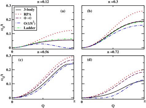
Figure 2: Spin-wave dispersion in the 1D system: comparison of the full three–body variational calculation (solid curve) to the different approximations discussed in the text. $J/t=10$.

For very small electron concentrations ($n=0.12$ in Figs. 2 and 3), the carrier–magnon scattering tends to soften the spin wave dispersion close to the zone boundary, consistent with previous results. wurth ; chubukov This can be seen by comparing in Figs. 2(a) and 3(a) the RPA dispersion with the different calculations of the carrier–magnon scattering effects. It is important to note that, despite the softening, the spin wave dispersion does not become negative (unstable) close to the zone boundary for very low concentrations. This softening may be interpreted as a remnant in the thermodynamic limit of the failure of the RPA for $N_{e}=1$, where Eq. (II.1) gives the exact solution. Indeed, for $N_{e}=1$, the magnon energy is of $O(1/N^{2})$, while the RPA gives $O(1/N)$ energies. Furthermore, for low concentrations, the $\Phi\neq 0,\Psi\neq 0$ and $\Phi=0,\Psi\neq 0$ variational calculations give results similar to the ladder approximation (the corresponding curves almost overlap in Figs. 2(a) and 3(a)). This indicates that the three–body correlations are weak for very low concentrations. This result can be understood by noting that the last term in Eq. (17) (and Eq. (A)), which describes the hole–magnon multiple scattering contribution, is suppressed for small $n$. Indeed, with decreasing $n$ and Fermi energy $E_{F}$, the phase space available for the hole to scatter decreases relative to the phase space available for electron scattering. As a result, the electron–magnon scattering channel (electron ladder diagrams) dominates. On the other hand, the difference between the above dispersions and the RPA is strong, while the differences from the $O(1/S^{2})$ (Born scattering) result are noticable even for very small $n$ (Figs. 2(a) and 3(a)). The latter differences come from the multiple electron–magnon and hole–magnon scattering processes. In 1D, the $O(1/S^{2})$ result fails qualitatively for very low ($n=0.12$ in Fig. 2) and very high ($n\geq 0.8$) electron concentrations. For such concentrations, the $O(1/S^{2})$ dispersion becomes negative (unstable) at the zone bondary. This zone boundary instability persists even in the strong coupling limit $J\rightarrow\infty$ but is absent in all our variational results.

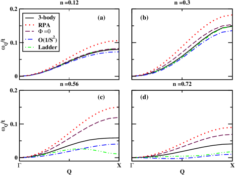
Figure 3: Spin-wave dispersion in the 2D system along the direction $\Gamma-X$ for the same parameters as in Fig. 2: comparison of the full three–body variational calculation (solid curve) to the different approximations discussed in the text.

With increasing electron concentration, the spin wave energies and stiffness initially increase (compare the $n=0.12$ and $n=0.3$ dispersions in Figs. 2 and 3). Fig. 4 shows $D(n)$, obtained by fitting the quadratic behavior $D(n)Q^{2}$ to the long wavelength numerical dispersions, for finite exchange interaction $J/t=10$. As can be seen in Fig. 4, the RPA predicts an initial increase of the spin wave stiffness with $n$ followed by a decrease. However, the carrier–magnon scattering reduces the spin wave stiffness and changes the above concentration dependence significantly, especially in 2D and 3D (see Fig. 4). The difference from the RPA behavior is particularly striking for the $O(1/S^{2})$ contribution to $D(n)$. The latter is significantly suppressed as compared to the rest of the approximations of carrier–magnon scattering. This particularly strong softening indicates that the $O(1/S^{2})$ result significantly underestimates $T_{c}$ and the stability of the fully polarized ferromagnetic state. We note that, due to the variational nature of the full three–body calculation, the exact stiffness will be smaller (softer) than the corresponding results of Fig.4 (solid curve).

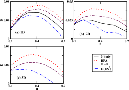
Figure 4: Spin wave stiffness for $J=10t$ as function of electron concentration and system dimensionality.

As the electron concentration increases, we see from Figs. 2 and 3 that the different approximations start to deviate substantially from each other. This is clear for the 2D system (Fig. 3), while in 1D the differences develop for higher electron concentrations. Compared to the full three–body variational calculation ($\Phi\neq 0,\Psi\neq 0$), the ladder and $O(1/S^{2})$ (non-variational) approximations give softer spin wave energies, while the variational $\Phi=0,\Psi\neq 0$ and RPA ($\Phi=\Psi=0$) wavefunctions give higher spin wave energies. The large differences between the above dispersions point out the importat role of carrier–magnon correlations for such electron concentrations. The difference between the full three–body calculation (or the $\Phi=0,\Psi\neq 0$ calculation) and the ladder approximation in Figs. 3(c) and 3(d) shows that the three–body correlations are signifcant, while the differences from the $O(1/S^{2})$ result show the importance of the multiple carrier–magnon scattering processes (vertex corrections). One can conclude from the above comparisons that the Fermi sea hole–magnon scattering cannot be neglected for such concentrations. Furthermore, as can be seen in Fig. 3, the different aproximations bound the full three–body result. This is particularly useful for the 3D system, where the full three–body variational calculation could only be performed for relatively small $N^{d}$ lattices with $N\sim 10$ (due to the large number of variational parameters $\Psi_{{\bf\alpha}{\bf\nu}}^{{\bf Q}}$). On the other hand, Fig. 5 shows the spin wave dispersions for a rather large ($50^{3})$ 3D lattice, obtained by using the RPA, $O(1/S^{2})$, and $\Phi=0,\Psi\neq 0$ approximations. By comparing the spin wave dispersions in Figs. 5 and 3, obtained for the same parameters, we see that the trends as function of $n$ are qualitatively similar in the 2D and 3D systems.

The differences between the approximations studied here (which are due to the correlations) are very pronounced in the electron concentration range $0.5\leq n\leq 0.8$ for intermediate exchange interaction values, i.e. in the parameter regime relevant to the manganites. This can be seen more clearly in Fig. 6, which shows the 2D spin wave dispersions obtained with the different approximations along the main directions in the Brillouin zone for the typical parameters $n=0.7,J=8t$. Fig. 6 compares the dispersions along the directions $(0,0)\rightarrow(\pi,0)$ ($\Gamma-X$), $(\pi,0)\rightarrow(\pi,\pi)$ ($X-M$), and along the diagonal $(0,0)\rightarrow(\pi,\pi)$ ($\Gamma-M$). The discrepancies between the different approximations are very large along $\Gamma-X$ but much smaller along the other directions. For example, the RPA fails completely along the direction $\Gamma-X$, where the full three–body calculation shows a striking spin wave softening that is most pronounced close to the $X$ point. Such a strong effect, much stronger than the softening at small $n$, only occurs for intermediate electron concentrations $0.4<n\leq 0.7$ and is underestimated by the $\Phi=0,\Psi\neq 0$ variational calculation. On the other hand, the $O(1/S^{2})$ dispersion for the parameters of Fig. 5 shows instability at long wavelengths (negative stiffness) rather than softening at the zone boundary.

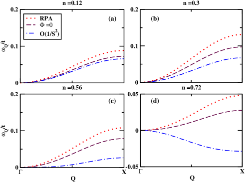
Figure 5: Spin wave dispersions in 3D for $J/t=10$ and electron concentrations similar to Figs. 2 and 3.

To see the origin of the above spin wave softening, we show in Fig. 7 the spin wave dispersion for a slightly smaller $J/t$ than in Fig 6. The spin wave energy now becomes negative in the vicinity of the $X$ point, while the magnon stiffness remains positive. This variational result allows us to conclude instability of the fully polarized ferromagnetic state due to the $X$ point magnons. The strong zone boundary softening is a precursor to this instability. Fig. 7 also compares the full three–body and RPA calculations for two different values of $N$ with fixed $n$. For $n=0.7$, our results have converged reasonably well even for $N\sim 10$ and thus reflect the behavior in the thermodynamic limit.

The above zone boundary instability occurs in 2D and 3D for intermediate electron concentrations ($0.4\leq n\leq 0.7$ for the 2D three–body calculation), where a strong magnon softening and short magnon lifetimes were observed in the manganites. soft-exp-1 ; soft-exp-2 ; soft-exp-3 ; soft-exp-4 ; endoh ; soft-2D-1 ; soft-2D-2 Although the other approximations can also give an instability, this occurs within a more limited range of $n$ and $J$ than for the full three–body calculation (discussed further below). The magnitude and concentration dependence of the softening also depends on the local Hubbard repulsion ($H_{U}$) and direct superexchange ($H_{super}$) interactions and the bandstructure (to be considered elsewhere). We note that spin wave softening at the zone boundary of electronic origin was obtained before within the one–orbital Hamiltonian for finite values of $J/t$ by including these additional effects. golosov ; mochena The main difference here is that our calculation is variational (and thus allows us to draw definite conclusions by guaranteeing that the exact magnon energies are even softer than the calculated values) and our effect was obtained by using the simplest possible Hamiltonian ($H_{U}=H_{super}=0$).

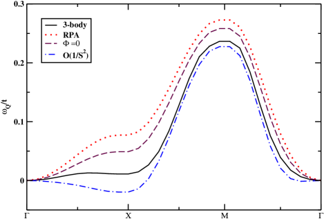
Figure 6: Spin wave dispersion along the different directions in Brillouin zone for $n=0.7,J=8t$: Comparison of the different approximations.

It is important to note here that the strong magnon softening and instability only occur for finite values of $J/t$ and disappear in the strong coupling limit $J\rightarrow\infty$. This can be seen in Fig. 8, which compares the 2D magnon dispersions for $n=0.7$ and different values of $J/t>1$ with the result obtained by expanding Eqs.(17) and (5) in the limit $J\rightarrow\infty$. As can be seen in Fig.8, the zone boundary magnon softening disappears with increasing $J/t$. The magnon dispersions converge slowly to the strong coupling result, which is reached only for $J/t\sim 1000$. Since the typical exchange interaction values in the manganites are of the order of $J/t\leq 10$, we conclude that the manganites are far from the $J\rightarrow\infty$ limit. Noting in Fig.8 that the zone boundary magnon softening has disappeared completely for $J/t\geq 20$, we see that the finite $J/t$ effects play an important role in the manganite spin dynamics.

We now turn to the 3D system, where the full three–body variational calculation faces computational difficulties due to the large number of variational parameters $\Psi^{{\bf Q}}_{{\bf\alpha}{\bf\nu}}$. As can be seen in Fig. 7, in the 2D system the magnon dispersion results for $n=0.7$ have already converged reasonably well for $N\sim 10$. We therefore expect that, in 3D, a calculation for a $N\times N\times N$ lattice with $N\sim 10$ should give reasonable results. Fig.9 show the 3D magnon dispersions obtained this way for $N=8$, $n\sim 0.7$, and $J/t=14$ using the different approximations. Fig. 9 shows similar 3D magnon behavior as in the 2D system (Fig. 5): magnon softening close to the $X$ point and significant deviations between the different approximations along $\Gamma-X$ even for this relatively large $J/t=14$. Similar to the 2D and 1D systems, the $O(1/S^{2})$ dispersion and the carrier–localized spin scattering ($\Phi=0,\Psi\neq 0$) variational results bound the full three–body magnon dispersion.

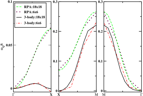
Figure 7: Spin wave dispersion for a $N\times N$ 2D lattice along different directions ($n=0.7,J=7.5t$). Convergence with system size $N$ is very good for this $n$.

Next we turn to the stability of the fully polarized half metallic ferromagnetic state. Our results show two different instabilities due to the exchange interaction ($H_{U}=H_{super}=0$). The first is the $X$–point zone boundary instability discussed above, which occurs in 2D and 3D for intermediate electron concentrations. For low or high electron concentrations (for all concentrations in 1D), we find a second instability with respect to long wavelength spin waves (negative magnon stiffness) similar to previous calculations. In this case, the minimum magnon energy occurs at a finite momentum value instead of ${\bf Q}=0$. This momentum increases with $n$ and becomes $\pi$ at $n=1$ (antiferromagnetic order at half filling). This result implies instability to a spiral state, while the system can further lower its energy by phase separating. dagotto ; papanico Due to the variational nature of our calculation, it is guaranteed that, if the magnon energy becomes negative for $J=J_{c}(n)$, the ground state of the Hamiltonian $H$ for all $J<J_{c}(n)$ is not the half metallic state $|F\rangle$. The phase diagrams of Fig. 10 describe the stability of this state against spin wave excitations. The most striking feature in Fig. 10 is the large shift (increase) of the ferromagnetic phase boundary, $J_{c}(n)$, as compared to the RPA, due to the carrier–magnon scattering. Furthermore, the different approximations of the carrier–magnon scattering lead to significant differences in $J_{c}(n)$. By comparing the shape of $J_{c}(n)$ between the 1D and 2D/3D systems, we see that, in the latter case, $J_{c}(n)$ develops a plateau–like shape within an intermediate concentration regime (see Fig. 10(d)). This feature is absent in the 1D system, where there is no zone boundary instability. This plateau occurs for $0.4<n\leq 0.7$ in 2D (full three–body calculation) and for $0.25<n<0.6$ in 3D ($\Phi=0,\Psi\neq 0$ three–body calculation). It is much less pronounced for the $O(1/S^{2})$ and RPA calculations

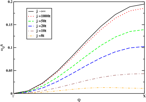
Figure 8: Spin wave dispersion in 2D, obtained from the full three–body calculations, for $n=0.7$ and increasing values of $J/t$. Convergence to the strong coupling limit is slow.

For small $n$, $J_{c}(n)$ is small, implying enhanced stability of the ferromagnetic state in the concentration regime relevant, e.g., to III-Mn-V semiconductors.III-V-1 ; III-V-2 This stability is a remnant of the fact that, in the exactly solvabe limit $N_{e}=1$, the ferromagnetic state $|F\rangle$ is the ground state for all values of $J/t$. $J_{c}(n)$ increases more slowly with $n$ in 1D than in 2D and 3D. This implies enhanced stability of the fully polarized ferromagnetic state, partly due to the lack of zone boundary instability in 1D. Fig. 10(d) shows the 2D phase diagrams for the electron concentrations relevant to the manganites. The full three–body variational calculation gives $J_{c}(n)\sim 7-8t$ in this regime, close to the high end of the values quoted in the literature. dagotto Therefore, the simple double exchange Hamiltonian predicts that the manganites lie in a regime that is close to the instability of the ferromagnetic state. In this regime, the correlations, vertex corrections, and finite $J$ effects play an important role in the spin dynamics.

Fig. 10 also compares the phase diagrams obtained by using the different approximations implemented here. The $O(1/S^{2})$ calculation underestimates the stability of the fully polarized ferromagnetic state, while the RPA and carrier–localized spin scattering ($\Phi=0,\Psi\neq 0$) variational results overstimate the stability. For low concentrations $n\leq 0.3$, all the different treatments of the carrier–magnon scattering predict a similar ferromagnetic phase bounday. It is clear from Fig. 10(d) that, in the electron concentration regime $0.5\leq n\leq 0.8$ relevant to the manganites, the RPA significantly overestimates the stability of the ferromagnetic state. For example, for $n\sim 0.5$, the RPA underestimates $J_{c}(n)$ by 100$\%$ as compared to the full three–body variational calculation. Finally, close to half filling $n=1$, the two variational results give magnon energies similar to the RPA, which becomes exact for $n=1$. On the other hand, the $O(1/S^{2})$ approximation fails in this high concentration regime.

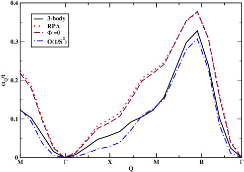
Figure 9: Spin wave dispersion for a $N\times N\times N$ 3D lattice along different directions ($n=0.7,J=14t$, and $N=8$). $\Gamma=(0,0,0),X=(\pi,0,0),M=(\pi,\pi,0),R=(\pi,\pi,\pi)$.

Finally we discuss the relevance of our calculation to the spin wave dispersion observed experimentally in the quasi–2D and 3D manganites. The experimental results are typically analyzed by fitting the short range Heisenberg dispersion to the long wavelength experimental dispersion and then comparing the two close to the zone boundary. sw-exp-1 ; soft-exp-1 ; soft-exp-2 ; soft-exp-3 ; soft-exp-4 ; endoh ; 2D-mang ; soft-2D-1 ; soft-2D-2 This comparison showed that the Heisenberg model fails to describe the experimental results in the overdoped manganites (typically for $0.5\leq n\leq 0.7$), but fits well in the underdoped samples ($n>0.7$). This failure is due to the strong magnon softening close to the zone boundary ($X$–point), soft-exp-1 ; soft-exp-2 ; soft-exp-3 ; soft-exp-4 ; endoh ; soft-2D-1 ; soft-2D-2 whose physical origin is currently under debate. soft-exp-1 ; soft-exp-2 ; soft-exp-3 ; soft-exp-4 ; endoh ; soft-2D-1 ; soft-2D-2 ; khal ; solovyev ; mochena Here we compare our numerical results with the Heisenberg dispersion $\omega^{Heis}_{{\bf Q}}$, obtained by fitting to the long wavelength numerical results, by introducing the parameter $\Delta=\omega^{Heis}_{X}/\omega_{X}-1,$ where $\omega^{Heis}_{X}$ and $\omega_{X}$ are the Heisenberg and numerical magnon energies calculated at the $X$–point. $|\Delta|$ thus measures the magnitude of the deviations from Heisenberg behavior at the zone boundary. For example, $|\Delta|\sim 1$ means $100\%$ deviation, $\Delta>0$ means magnon softening at the zone boundary, as compared to the Heisenberg dispersion with the same stiffness, while $\Delta<0$ implies zone boundary hardening. Fig. 11 compares $\Delta(n)$ obtained from our different approximations. With the exception of small values of $J/t$, the RPA gives small deviations from Heisenberg behavior, mostly a hardening at the zone boundary ( $\Delta<0$, see Fig. 10), and predicts a weak concentration dependence of $\Delta(n)$. This similarity between the RPA and Heisenberg dispersions is expected for $J\gg t$ since the two coincide in the strong coupling limit $J\rightarrow\infty$ (see Eq.(3)).

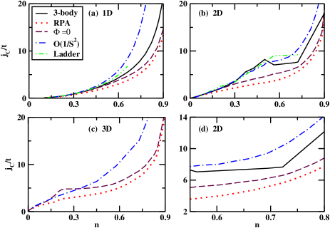
Figure 10: Phase diagram due to the spin wave instability and comparison between the different approximations discussed in the text. (a) 1D system, (b) 2D system, (c) 3D system, and (d) 2D system in the electron concentration range relevant to the manganites.

The magnon–electron scattering leads to larger deviations from Heisenberg ferromagnet spin dynamics and enhances $\Delta(n)$ (see Figs. 11(a) and 11(b) for 2D and 3D respectively). In order to compare with the experiment, the value of $J/t$ must be chosen so that $|F\rangle$ is stable up to $n\sim 0.8$, where a metallic ferromagnetic state is observed experimentally. For $J/t\sim 10$, this is the case for the full three–body calculation, while larger values of $J/t$ are required to achieve stability for $n\sim 0.8$ with respect to the $O(1/S^{2})$ magnons. Figs. 11(a) and 11(b) compare the behavior of $\Delta(n)$ for the different approximations in the 2D and 3D systems respectively. The $O(1/S^{2})$ calculation gives magnon hardening rather than softening in the concentration range of interest, similar to the strong coupling results of Ref. chubukov, . This is in contrast to $\Delta(n)$ obtained by using the full three–body calculation, shown in Fig. 11(a) for the 2D system. In this case, the magnon hardening for $n<0.5$ ($\Delta<0$) changes to magnon softening for $0.5<n<0.7$ ($\Delta>0$) and then back to a small magnon hardening for $n>0.7$. This behavior with $n$ is consistent with the experimental trends. Although magnon softening at the $X$ point can be obtained using other approximations, the full three–body calculation gives such an enhanced effect within the range of intermediate electron concentrations of interest and for values of $J/t$ such that the fully polarized ferromagnetic state is stable for $0.5\leq n\leq 0.8$ (where it is observed experimentally). The above behavior of $\Delta(n)$ is not reproduced in the strong coupling limit $J\rightarrow\infty$, where magnon hardening is obtained. It arises from the interplay of the $X$–point instability and the plateau–like shape of $J_{c}(n)$, Fig.10, induced by the correlations. On the other hand, for $J=10t$, the carrier–localized spin scattering approximation ($\Phi=0,\Psi\neq 0$ variational wavefunction) gives $\Delta(n)$ that, more or less, follows the RPA behavior (see Figs. 11(a) and 11(b)). As $J/t$ decreases, magnon softening, $\Delta>0$, can also be obtained with this approximation over a range of electron concentrations in both 2D and 3D (see Figs. 11(c) (2D) and 11(d) (3D)). However, for such $J/t$, the ferromagnetic state is unstable for $n>0.6$, i.e. in a regime where ferromagnetism is observed experimentally. We expect that the precise behavior of $\Delta(n)$ in the realistic materials will also depend on $H_{U}$, $H_{super}$, and the bandstructure effects (to be studied elsewhere). Here we point out that at least three–body correlations must be included for a meaningful comparison to the experiment.

Figure 11: Deviation $\Delta(n)$, defined in the text, from Heisenberg ferromagnet spin dynamics in the 2D and 3D systems for fixed $J/t=10$ and different electron concentrations.

IV Conclusions

In this paper we presented a nonperturbative variational calculation of the effects of magnon–Fermi sea pair correlations on the spin wave dispersion for the simplest possible double exchange Hamiltonian. Our theory treats exactly all three–body long range correlations between an electron, a Fermi sea hole, and a magnon excitation. We achieved this by using the most general variational wavefunction that includes up to one Fermi sea pair excitations. Since the contribution of multipair Fermi sea excitations is suppressed by powers of $1/S$, one could alternatively think of our calculation as putting the $O(1/S^{2})$ result, which treats the one Fermi sea pair contribution perturbatively within the Born approximation, on a variational nonperturbative basis. Our theory (i) becomes exact in the two limits of one and $N^{d}$ electrons and should therefore interpolate well between the low concentration and half filling limits, (ii) converges well with system size and thus applies to the thermodynamic limit, (iii) becomes exact in the atomic limit ($t$=0), conserves momentum exactly, and treats both short and long range correlations on equal basis; it should therefore interpolate well between the strong and weak coupling limits, which is important given the relatively small values of $J/t$ in the manganites, and (iv) contains the well known $O(1/S^{2})$ and RPA results as limiting cases. In this paper we studied, among others, (i) the shape of the spin wave dispersion and ferromagnetic phase boundary for different system dimensionalities (1D, 2D, and 3D), (ii) the deviations from the strong coupling double exchange limit, and (iii) the role of up to three–body correlations and nonperturbative vertex corrections on the spin dynamics. By comparing the full three–body variational calculation to a number of approximations (RPA, 1/S expansion, ladder diagram treatment of two-body correlations, and carrier–localized spin rather than carrier–magnon scattering), we showed that the correlations play an important role on the spin excitation spectrum, the stability of the ferromagnetism, and the shape of the ferromagnetic phase boundary in the parameter range relevant to the manganites. Importantly, the correlations lead to spin dynamics that differs strongly from that of the short range Heisenberg ferromagnet for intermediate electron concentrations.

Our main results can be summarized as follows. First, the different approximations lead to substantial differences in the spin wave dispersion and ferromagnetic phase boundary for electron concentrations above $n\sim 0.3$ and intermediate values of $J/t$, which includes the parameter range relevant to the manganites. These large differences come from the correlations, which cannot be neglected, and imply that variational calculations should be used if possible in order to draw definite conclusions. Second, we find that, depending on $n$, there are two possibile instabilities of the ferromagnetic state toward spin wave excitations: instability driven by a negative spin stiffness and instability at large momenta, close to the $X$–point zone boundary, with positive stiffness. The latter instability only occurs in the 2D and 3D systems, for electron concentrations $n\leq 0.7$ and finite values of $J$. The three–body carrier–magnon correlations enhance this effect. As a precursor to the above zone boundary instabilty, we find a strong magnon softening at the $X$–point, which should be accompanied by short magnon lifetimes. Third, by comparing to the Heisenberg dispersion obtained by fitting to the long wavelength numerical results, we find strong deviations from the spin dynamics of the short range Heisenberg model. By choosing the exchange interaction so that the fully polarized ferromagnetic state is stable up to $n>0.8$ as in the experiment, we show that the full three–body 2D calculation gives strong magnon softening at the $X$ point for $0.5\leq n\leq 0.7$, which changes into a small hardening for $n>0.7$. This is similar to the behavior observed in the manganites. Our work provides new insight into the spin dynamics in the manganites and can be extended to treat related ferromagnetic systems (such as e.g. the III-Mn-V magnetic semiconductors) that are far from the double exchange strong coupling limit. Our calculations imply that the metallic ferromagnetic state in the manganites should be viewed as a strongly correlated state. Finally, the carrier–magnon correlations studied here can also play an important role in the ultrafast relaxation dynamics of itinerant ferromagnetic systems, which is beginning to be explored by using ultrafast magneto-optical pump–probe spectroscopy. ultrafast-per ; ultrafast-cmr ; ultrafast-ferro

We thank N. Papanicolaou for very useful discussions. This work was supported by the EU Research Training Network HYTEC (HPRN-CT-2002-00315).

Appendix A

In this Appendix we present the variational equations that determine the wavefunction amplitudes $X^{{\bf Q}}$, $\Psi^{{\bf Q}}$, and $\Phi^{{\bf Q}}$. These are obtained by minimizing the variational energy $\langle F|M_{{\bf Q}}HM^{\dagger}_{{\bf Q}}|F\rangle$, where $M^{{\dagger}}_{{\bf Q}}$ is given by Eq.(II.1), with respect to the above variational amplitudes. The normalization condition $\langle F|M_{{\bf Q}}M^{\dagger}_{{\bf Q}}|F\rangle=1$ is enforced via a Lagrange multiplier, which coincides with the variational magnon energy $\omega_{{\bf Q}}$. Similar to the three–body Fadeev equations, the resulting variational equations are equivalent to solving the Schrödinger equation within the subspace spanned by the states $S_{{\bf Q}}^{-}|F\rangle$ and $c_{{\bf Q}+{\bf\nu}\downarrow}^{{\dagger}}c_{{\bf\nu}\uparrow}|F\rangle$, which describe all possible configurations with one reversed spin and no Fermi sea excitations, and the magnon–Fermi sea pair states $c_{{\bf\alpha}\uparrow}^{{\dagger}}c_{{\bf\nu}\uparrow}S_{{\bf Q}+{\bf\nu}-{\bf\alpha}}^{-}|F\rangle$ and $c_{{\bf\alpha}\uparrow}^{{\dagger}}c_{{\bf\nu}\uparrow}c_{{\bf Q}+{\bf\mu}+{\bf\nu}-{\bf\alpha}\downarrow}^{{\dagger}}c_{{\bf\mu}\uparrow}|F\rangle$ to which a magnon or spin flip excitation can scatter with the simultaneous excitation of a Fermi sea pair. We note that the above momentum space basis ensures the conservation of momentum and total spin. The explicit form of the variational equations is obtained after straighforward algebra by projecting the Schrödinger equation $[H,M^{\dagger}_{{\bf Q}}]|F\rangle=\omega_{{\bf Q}}|F\rangle$ in the above basis after calculating the commutator $[H,M^{\dagger}_{{\bf Q}}]$ by using Eq.(II.1) for $M^{\dagger}_{{\bf Q}}$ and noting that $H|F\rangle=0$ ( we take the energy of $|F\rangle$ as zero). The variational equation that gives the energy $\omega_{{\bf Q}}$ reads

$$\omega_{{\bf Q}}=\frac{Jn}{2}-\frac{J}{2N}\sum_{{\bf\nu}}X^{{\bf Q}}_{{\bf\nu}}+\frac{J}{2N}\sum_{{\bf\alpha}{\bf\nu}}\Psi^{{\bf Q}}_{{\bf\alpha}{\bf\nu}}.$$ (10)

The last term in the above equation describes the contribution due to the carrier–magnon scattering. The first two terms on the rhs give the RPA magnon energy if $X^{{\bf Q}}_{{\bf\nu}}$ is substituted by its RPA value, obtained for $\Psi^{{\bf Q}}=0$. The carrier–magnon scattering renormalizes $X^{{\bf Q}}_{{\bf\nu}}$ as compared to the RPA result:

$$(JS+\varepsilon_{{\bf\nu}+{\bf Q}}-\varepsilon_{{\bf\nu}}-\omega_{{\bf Q}})\,X^{{\bf Q}}_{{\bf\nu}}=JS\left[1+\sum_{\alpha}\Psi^{{\bf Q}}_{{\bf\alpha}{\bf\nu}}\right].$$ (11)

The first term on the rhs of the above equation gives the RPA contribution to $X^{{\bf Q}}_{{\bf\nu}}$, while the second term, as well as the correlation contribution to the magnon energy $\omega_{{\bf Q}}$, describe the effects of the magnon–carrier scattering. The RPA is obtained from Eqs. (10) and (11) after setting $\Psi^{{\bf Q}}=\Phi^{{\bf Q}}=0$:

$$\omega_{{\bf Q}}^{RPA}=\frac{Jn}{2}-\frac{J}{2N}\sum_{{\bf\nu}}X_{{\bf\nu}}^{{\bf Q}RPA},$$ (12)

$$X^{{\bf Q}RPA}_{{\bf\nu}}=\frac{JS}{JS+\varepsilon_{{\bf\nu}+{\bf Q}}-\varepsilon_{{\bf\nu}}-\omega^{RPA}_{{\bf Q}}}.$$ (13)

This full RPA result can also be obtained as the zeroth order contribution to an expansion in powers of 1/L, where $L$ is the number of electron flavors and corresponding degenerate electron bands. papanico

The scattering amplitude $\Psi^{{\bf Q}}$ is determined by the variational equation

$$\left(\omega_{{\bf Q}}-\frac{Jn}{2}+\varepsilon_{{\bf\nu}}-\varepsilon_{{\bf\alpha}}\right)\Psi^{{\bf Q}}_{{\bf\alpha}{\bf\nu}}=\frac{J}{2N}\left(1-X^{{\bf Q}}_{{\bf\nu}}\right)$$

$$+\frac{J}{2N}\sum_{{\bf\alpha}^{\prime}}\Psi^{{\bf Q}}_{{\bf\alpha}^{\prime}{\bf\nu}}-\frac{J}{2N}\sum_{{\bf\nu}^{\prime}}\Psi^{{\bf Q}}_{{\bf\alpha}{\bf\nu}^{\prime}}-\frac{J}{2N}\sum_{{\bf\nu}^{\prime}}\Phi^{{\bf Q}}_{{\bf\alpha}{\bf\nu}^{\prime}{\bf\nu}}.$$ (14)

The first term on the rhs of the above equation gives the Born scattering approximation contribution to the carrier–magnon scattering amplitude, which is the only one that contributes to $O(1/S^{2})$. The next two terms describe the effects of the multiple electron–magnon (second term) and hole magnon (third term) scattering. Finally, the last term comes from the electronic contribution to the scattered magnon, i.e. from the coherent excitation of a spin–$\uparrow$ electron to the spin–$\downarrow$ band. The amplitude $\Phi^{Q}$ of the latter contribution to Eq.(II.1) is given by the variational equation

$$\left(JS+\varepsilon_{{\bf Q}+{\bf\mu}+{\bf\nu}-{\bf\alpha}}-\varepsilon_{{\bf\mu}}+\varepsilon_{{\bf\alpha}}-\varepsilon_{{\bf\nu}}-\omega_{{\bf Q}}\right)\Phi^{{\bf Q}}_{{\bf\alpha}{\bf\nu}{\bf\mu}}=$$

$$JS\left(\Psi^{{\bf Q}}_{{\bf\alpha}{\bf\nu}}-\Psi^{{\bf Q}}_{{\bf\alpha}{\bf\mu}}\right).$$ (15)

We note that, in the strong coupling limit $J\rightarrow\infty$, $\Phi^{{\bf Q}}_{{\bf\alpha}{\bf\nu}{\bf\mu}}\rightarrow\Psi^{{\bf Q}}_{{\bf\alpha}{\bf\nu}}-\Psi^{{\bf Q}}_{{\bf\alpha}{\bf\mu}}$ and the last two terms in Eq. (II.1) describe the scattering of a Fermi sea pair with the strong coupling RPA magnon created by the total spin lowering operator $S_{{\bf Q}}^{-}+\frac{1}{\sqrt{N}}\sum_{{\bf\nu}}c_{{\bf Q}+{\bf\nu}\downarrow}^{{\dagger}}c_{{\bf\nu}\uparrow}$. Our general wavefunction Eq. (II.1) does not assume an RPA magnon and includes corrections to the strong coupling limit that are important for the values of $J/t$ relevant to the manganites.

A closed equation for the carrier–magnon scattering amplitude $\Psi^{{\bf Q}}$ can be obtained by substituting in Eq. (14) the expressions for $\Phi^{{\bf Q}}$ and $X^{{\bf Q}}$ obtained from Eqs. (A) and (11). Defining the excitation energy

$$\Delta_{{\bf\alpha}{\bf\nu}}^{{\bf Q}}=\omega_{{\bf Q}}+\varepsilon_{{\bf\nu}}-\varepsilon_{{\bf\alpha}}$$

$$-\frac{J}{2N}\sum_{\nu^{\prime}}\frac{\varepsilon_{{\bf Q}+{\bf\nu^{\prime}}+{\bf\nu}-{\bf\alpha}}-\varepsilon_{{\bf\nu}^{\prime}}+\varepsilon_{{\bf\alpha}}-\varepsilon_{{\bf\nu}}-\omega_{{\bf Q}}}{JS+\varepsilon_{{\bf Q}+{\bf\nu^{\prime}}+{\bf\nu}-{\bf\alpha}}-\varepsilon_{{\bf\nu}^{\prime}}+\varepsilon_{{\bf\alpha}}-\varepsilon_{{\bf\nu}}-\omega_{{\bf Q}}}$$ (16)

we thus obtain the following equation:

$$\Delta^{{\bf Q}}_{{\bf\alpha}{\bf\nu}}\Psi^{{\bf Q}}_{{\bf\alpha}{\bf\nu}}=\frac{J}{2N}\frac{\varepsilon_{{\bf\nu}+{\bf Q}}-\varepsilon_{{\bf\nu}}-\omega_{{\bf Q}}}{JS+\varepsilon_{{\bf\nu}+{\bf Q}}-\varepsilon_{{\bf\nu}}-\omega_{{\bf Q}}}\left[1+\sum_{{\bf\alpha}^{\prime}}\Psi^{{\bf Q}}_{{\bf\alpha}^{\prime}{\bf\nu}}\right]$$

$$-\frac{J}{2N}\sum_{{\bf\nu}^{\prime}}\Psi^{{\bf Q}}_{{\bf\alpha}{\bf\nu}^{\prime}}\frac{\varepsilon_{{\bf Q}+{\bf\nu}+{\bf\nu}^{\prime}-{\bf\alpha}}-\varepsilon_{{\bf\nu}^{\prime}+\varepsilon_{{\bf\alpha}}-\varepsilon_{{\bf\nu}}}-\omega_{{\bf Q}}}{JS+\varepsilon_{{\bf Q}+{\bf\nu}+{\bf\nu}^{\prime}-{\bf\alpha}}-\varepsilon_{{\bf\nu}^{\prime}}+\varepsilon_{{\bf\alpha}}-\varepsilon_{{\bf\nu}}-\omega_{{\bf Q}}}.$$ (17)

The above equation describes up to three–body correlations between the magnon and a Fermi sea pair. The first term on the rhs describes the bare carrier–magnon scattering amplitude. This is renormalized by the multiple scattering of a Fermi sea electron (second term on the rhs) and a Fermi sea hole (last term on the rhs). These two contributions describe vertex corrections of the carrier–magnon interaction. Eqs.(10) and (17) were solved iteratively until convergence for the spin wave energy was reached.

Appendix B

In this Appendix we identify the three–body correlation contribution to the carrier–magnon scattering amplitude $\Psi^{{\bf Q}}$, Eq. (17), and distinguish it from the two–body multiple scattering contributions.

We note from Eq. (17), that $\Psi^{{\bf Q}}$ has the form

$$\Psi^{{\bf Q}}_{{\bf\alpha}{\bf\nu}}\ =\frac{J}{2N\Delta^{{\bf Q}}_{{\bf\alpha}{\bf\nu}}}\frac{\varepsilon_{{\bf\nu}+{\bf Q}}-\varepsilon_{{\bf\nu}}-\omega_{{\bf Q}}}{JS+\varepsilon_{{\bf\nu}+{\bf Q}}-\varepsilon_{{\bf\nu}}-\omega_{{\bf Q}}}+\frac{\Gamma^{e}_{{\bf\nu}}-\Gamma^{h}_{{\bf\alpha}{\bf\nu}}}{\Delta^{{\bf Q}}_{{\bf\alpha}{\bf\nu}}},$$ (18)

where we introduced the electron vertex function Eq.(6) and the hole vertex function

$$\Gamma^{h}_{{\bf\alpha}{\bf\nu}}=\frac{J}{2N}\sum_{{\bf\nu}^{\prime}}\Psi_{{\bf\alpha}{\bf\nu}^{\prime}}\frac{\varepsilon_{{\bf Q}+{\bf\nu}+{\bf\nu}^{\prime}-{\bf\alpha}}+\varepsilon_{{\bf\alpha}}-\varepsilon_{{\bf\nu}}-\varepsilon_{{\bf\nu}^{\prime}}-\omega_{{\bf Q}}}{JS+\varepsilon_{{\bf Q}+{\bf\nu}+{\bf\nu}^{\prime}-{\bf\alpha}}-\varepsilon_{{\bf\nu}^{\prime}}+\varepsilon_{{\bf\alpha}}-\varepsilon_{{\bf\nu}}-\omega_{{\bf Q}}}.$$ (19)

Substituting Eq. (18) into Eq. (6) we obtain after some algebra that

$$\Gamma^{e}_{{\bf\nu}} = \left[1-\frac{J}{2N}\frac{\varepsilon_{{\bf\nu}+{\bf Q}}-\varepsilon_{{\bf\nu}}-\omega_{{\bf Q}}}{JS+\varepsilon_{{\bf\nu}+{\bf Q}}-\varepsilon_{{\bf\nu}}-\omega_{{\bf Q}}}\sum_{{\bf\alpha}^{\prime}}\frac{1}{\Delta^{{\bf Q}}_{{\bf\alpha}^{\prime}{\bf\nu}}}\right]^{-1}\times$$ (20)

$$\left[\frac{J^{2}}{4N^{2}}\left(\frac{\varepsilon_{{\bf\nu}+{\bf Q}}-\varepsilon_{{\bf\nu}}-\omega_{{\bf Q}}}{JS+\varepsilon_{{\bf\nu}+{\bf Q}}-\varepsilon_{{\bf\nu}}-\omega_{{\bf Q}}}\right)^{2}\sum_{{\bf\alpha}^{\prime}}\frac{1}{\Delta^{{\bf Q}}_{{\bf\alpha}^{\prime}{\bf\nu}}}\right.$$

$$\left.-\frac{J}{2N}\frac{\varepsilon_{{\bf\nu}+{\bf Q}}-\varepsilon_{{\bf\nu}}-\omega_{{\bf Q}}}{JS+\varepsilon_{{\bf\nu}+{\bf Q}}-\varepsilon_{{\bf\nu}}-\omega_{{\bf Q}}}\sum_{{\bf\alpha}^{\prime}}\frac{\Gamma^{h}_{{\bf\alpha}^{\prime}{\bf\nu}}}{\Delta^{{\bf Q}}_{{\bf\alpha}^{\prime}{\bf\nu}}}\right].$$

The first factor on the rhs of the above equation comes from the electron–magnon two–body ladder diagrams summed to infinite order. The last term in the second factor describes the coupling of the electron–magnon and hole–magnon scattering channels. This coupling comes from the three–body correlations. An analogous equation for $\Gamma^{h}$ can be obtained by substituting Eq.(18) into Eq. (19). In the case of the simpler variational wavefunction $\Phi=0,\Psi\neq 0$, which describes the carrier–localized spin scattering contribution, the calculation of $\Gamma^{h}$ simplifies by noting from Eq.(14) and the definition Eq.(18) that $\Gamma^{h}_{{\bf\alpha}}=\Gamma^{h}_{{\bf\alpha}{\bf\nu}}$. The corresponding variational equation can be obtained by setting $\Phi^{{\bf Q}}=0$ in Eq. (14):

$$\Gamma^{h}_{{\bf\alpha}}=\left[1+\frac{J}{2N}\sum_{{\bf\nu}^{\prime}}\frac{1}{\Delta^{{\bf Q}}_{{\bf\alpha}{\bf\nu}^{\prime}}}\right]^{-1}\times$$

$$\left[\frac{J^{2}}{4N^{2}}\sum_{{\bf\nu}^{\prime}}\frac{\varepsilon_{{\bf\nu}^{\prime}+{\bf Q}}-\varepsilon_{{\bf\nu}^{\prime}}-\omega_{{\bf Q}}}{JS+\varepsilon_{{\bf\nu}^{\prime}+{\bf Q}}-\varepsilon_{{\bf\nu}^{\prime}}-\omega_{{\bf Q}}}\frac{1}{\Delta^{{\bf Q}}_{{\bf\alpha}{\bf\nu}^{\prime}}}+\frac{J}{2N}\sum_{{\bf\nu}^{\prime}}\frac{\Gamma^{e}_{{\bf\nu}^{\prime}}}{\Delta^{{\bf Q}}_{{\bf\alpha}{\bf\nu}^{\prime}}}\right].\ \$$ (21)

The first factor on the rhs comes from the hole–magnon ladder diagrams, while the coupling to $\Gamma^{e}$ comes from the three–body correlations.

References

- (1) See e.g. E. L. Nagaev, Phys. Rep. 346, 387 (2001) and references therein.
- (2) E. L. Nagaev, Phys. Rev. B 58, 827 (1998)
- (3) E. L. Nagaev, Sov. Physics Solid State, 11 (1970)
- (4) See e.g. J. König, J. Schliemann, T. Jungwirth, and A. H. MacDonald, in Electronic Structure and Magnetism of Complex Materials, eds. J. Singh and D. A. Papaconstantopoulos (Springer-Verlag, Berlin, 2002).
- (5) M. Berciu and R. N. Bhatt, Phys. Rev. B 66, 085207 (2002); P. M. Krstajic, F. M. Peeters, V. A. Ivanov, V. Fleurov, and K. Kikoin, Phys. Rev. B 70, 195215 (2004).
- (6) See e.g. Colossal Magnetoresistance Oxides, ed. Y. Tokura (Gordon Breach, Singapore, 2000) and references therein.
- (7) E. Dagotto, T. Hotta, and A. Moreo, Phys. Rep. 344, 1 (2001).
- (8) C. S. Zener, Phys. Rev. 82, 403 (1951); P. W. Anderson and H. Hasegawa, Phys. Rev. 100, 675 (1955); P. G. de Gennes, Phys. Rev. 100, 564 (1955); K. Kubo and N. Ohata, J. Phys. Soc. Jpn. 33, 21 (1972).
- (9) D. I. Golosov, Phys. Rev. Lett. 84, 3974 (2000); Phys. Rev. B 71, 014428 (2005); and references therein.
- (10) N. Shannon and A. V. Chubukov, Phys. Rev. B 65, 104418 (2002); J. Phys. Cond. Matt. 14, L235 (2002).
- (11) N. Furukawa, J. Phys. Soc. Jpn. 65, 1174 (1996).
- (12) X. Wang, Phys. Rev. B 57, 7427 (1998).
- (13) J. Zang. H. Röder, A. R. Bishop, and S. A. Trugman, J. Phys. Cond. Matt. 9, L157 (1997).
- (14) T. A. Kaplan and S. D. Mahanti, J. Phys. Cond. Matt. 9, L291 (1997).
- (15) T. A. Kaplan and S. D. Mahanti, Phys. Rev. Lett. 86, 3634 (2000).
- (16) T. Okabe, Phys. Rev. B 57, 403 (1998).
- (17) T. Okabe, Theor. Phys. 97, 21 (1997).
- (18) P. Wurth and E. Müller-Hartmann, Eur. Phys. J. B 5, 403 (1998).
- (19) L. M. Roth, Phys. Rev. Lett. 20, 1431 (1968); Phys. Rev. 186, 428 (1969); J. Phys. Chem. Solids 28, 1549 (1967).
- (20) See e.g. A. E. Ruckenstein and S. Schmitt–Rink, Int. J. Mod. Phys. B 3, 1809 (1989) and references therein.
- (21) B. S. Shastry, H. R. Krishnamurthy, and P. W. Anderson, Phys. Rev. B 41, 2375 (1990).
- (22) W. von der Linden and D. M. Edwards, J. Phys. : Condens. Matter 3, 4917 (1991).
- (23) T. G. Perring, G. Aeppli, S. M. Hayden, S. A. Carter, J. P. Remeika, and S.-W. Cheong, Phys. Rev. Lett. 77, 711 (1996).
- (24) H. Y. Hwang, P. Dai, S.-W. Cheong, G. Aeppli, D. A. Tennant, and H. A. Mook, Phys. Rev. Lett. 80, 1316 (1998).
- (25) P. Dai, H. Y. Hwang, J. Zhang, J. A. Fernandez-Baca, S.-W. Cheong, C. Kloc, Y. Tomioka, and Y. Tokura, Phys. Rev. B 61, 9553 (2000).
- (26) L. Vasiliu-Doloc, J. W. Lynn, A. H. Moudden, A. M. de Leon-Guevara, and A. Revcolevschi, Phys. Rev. B 58, 14913 (1998).
- (27) T. Chatterji, L. P. Regnault, and W. Schmidt, Phys. Rev. B 66, 214408 (2002).
- (28) Y. Endoh, H. Hiraka, Y. Tomioka, Y. Tokura, N. Nagaosa, and T. Fujiwara, Phys. Rev. Lett. 94, 017206 (2005).
- (29) T. Chatterji, L. P. Regnault, P. Thalmeier, R. Suryanarayanan, G. Dhalenne, and A. Revcolevschi, Phys. Rev. B 60, R6965 (1999).
- (30) N. Shannon, T. Chatterji, F. Ouchni, and P. Thalmeier, Eur. Phys. J. B 27, 287 (2002).
- (31) G. Khaliullin and R. Kilian, Phys. Rev. B 61, 3494 (2000).
- (32) I. V. Solovyev and K. Terakura, Phys. Rev. Lett. 82, 2959 (1999).
- (33) S–S Feng and M. Mochena, J. Phys. Cond. Matt. 17, 3895 (2005); F. Mancini, N. B. Perkins, and N. M. Plakida, Phys. Lett. A 284, 286 (2001).
- (34) J. Igarashi, M. Takahashi, and T. Nagao, J. Phys. Soc. Jpn 68, 3682 (1999); J. Igarashi, J. Phys. Soc. Jpn 54, 260 (1985).
- (35) I. E. Perakis and Y.–C. Chang, Phys. Rev. B 47, 6573 (1993); ibid 44, 5877 (1991); and references therein.
- (36) J. F. Mueller, A. E. Ruckenstein, and S. Schmitt–Rink, Phys. Rev. B 45, 8902 (1992); A. E. Ruckenstein and S. Schmitt–Rink, Phys. Rev. B 35, 7551 (1987); and references therein.
- (37) T. G. Perring, D. T. Adroja, G. Chaboussant, G. Aeppli, T. Kimura, and Y. Tokura, Phys. Rev. Lett. 87, 217201 (2001).
- (38) Y. Moritomo, A. Asamitsu, H. Kuwahara, and Y. Tokura, Nature 380, 141 (1996); H. Martinho, C. Rettori, D. L. Huber, J. F. Mitchell, and S. B. Oseroff, Phys. Rev. B 67, 214428 (2003).
- (39) See e.g. Y. Endoh and K. Hirota, J. Phys. Soc. Jpn 66, 2264 (1997).
- (40) M. Marder, N. Papanicolaou, and G. C. Psaltakis, Phys. Rev. B 41, 6920 (1990); L. R. Mead and N. Papanicolaou, Phys. Rev. B 28, 1633 (1983).
- (41) J. Chovan, E. G. Kavousanaki, and I. E. Perakis, cond-mat/0508178; Phys. Rev. Lett. (to be published).
- (42) Y. H. Ren, X. H. Zhang, G. Lüpke, M. Schneider, M. Onellion, I. E. Perakis, Y. F. Hu, and Q. Li, Phys. Rev. B 64, 144401 (2001).
- (43) M. Vomir, L. H. F. Andrade, L. Guidoni, E. Beaurepaire, and J.-Y. Bigot, Phys. Rev. Lett. 94, 237601 (2005); J.-Y. Bigot, L. Guidoni, E. Beaurepaire, and P. N. Saeta, Phys. Rev. Lett. 93, 077401 (2004).