General model for Apollonian networks

Abstract

We introduce a general deterministic model for Apollonian Networks in an iterative fashion. The networks have small-world effect and scale-free topology. We calculate the exact results for the degree exponent, the clustering coefficient and the diameter. The major points of our results indicate that (a) the degree exponent can be adjusted in a wide range, (b) the clustering coefficient of each individual vertex is inversely proportional to its degree and the average clustering coefficient of all vertices approaches to a nonzero value in the infinite network order, and (c) the diameter grows logarithmically with the number of network vertices.

I Introduction

In the past few years we have witnessed an upsurge in the research of a wide range of complex systems which can be described in terms of networks——vertices connected together by edges AlBa02 ; DoMe03 ; SaVe04 ; Ne03 . Various empirical studies have shown that most real-life systems exhibit the following three properties: power-law degree distribution BaAl99 , high clustering coefficient WaSt98 and small average path length (APL) which implies that their average intervertex distances grow logarithmically with the number of vertices or slower.

In order to mimic real-world systems, a wide variety of models have been proposed AlBa02 ; DoMe03 ; SaVe04 ; Ne03 , most of which are random. Randomness may be in line with the major features of real-life networks, but as mentioned by Barabási et al., it makes harder to gain a visual understanding of how networks are shaped, and how do different vertices relate to each other BaRaVi01 . Therefore, it would be of major theoretical interest to construct deterministic models having similar structural characteristics as systems in nature and society. A strong advantage of deterministic networks is that it is often possible to compute analytically their properties, which may be compared with empirical data from real-life systems. In the last few years, deterministic networks have been intensively studied BaRaVi01 ; CoOzPe00 ; CoSa02 ; DoGoMe02 ; JuKiKa02 ; CoFeRa04 ; RaBa03 ; No03 ; ZhWaHuCh04 ; IgYa05 ; ZhRoGo05 .

Recently, In relation to the problem of Apollonian packing, Andrade et al. introduced Apollonian networks AnHeAnSi05 which were also proposed by Doye and Massen in DoMa05 . Apollonian networks are part of a deterministic growing type of networks and have received much attention. Except their further properties ZhCoFeRo05 , stochastic versions ZhYaWa05 ; ZhRoCo05 and potential implications DoMa05 ; DoMa05b , many peculiar results about some famous models upon Apollonian networks have been found AnHeAnSi05 ; AnHe05 ; LiGaHe04 ; AnMi05 .

In this paper, we do an extensive study on Apollonian networks. In an iterative way we propose a general model for Apollonian networks by including a parameter. Apollonian networks AnHeAnSi05 ; DoMa05 ; ZhCoFeRo05 are special cases of the present model. The deterministic construction of our model enables one to obtain the analytic solution for the degree distribution, clustering coefficient and the diameter. Moreover, by tuning the parameter, we can obtain scale-free networks with a variety of degree exponents and clustering coefficient.

II Brief introduction to Apollonian networks

To define Apollonian networks, we first introduce Apollonian packing (see Fig. 1 for the case of two dimension). The classic two-dimensional Apollonian packing is constructed as follows. Initially three mutually touching disks are inscribed inside a circular space which is to be filled. The interstices of the initial disks and circle are curvilinear triangle to be filled. This initial configuration is called generation $t=0$. Then in the first generation $t=1$, four disks are inscribed, each touching all the sides of the corresponding curvilinear triangle. For next generations we simply continue by setting disks in the newly generated curvilinear triangles. The process is repeated indefinitely for all the new curvilinear triangles. In the limit of infinite generations we obtain the Apollonian packing, in which the circular space is completely filled with disks of various sizes. The translation from Apollonian packing construction to Apollonian network generation is quite straightforward: vertices of the network represent disks and two vertices are connected if the corresponding disks are tangent AnHeAnSi05 ; DoMa05 .

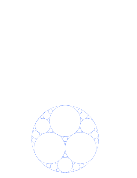
Figure 1: (Color online) A two-dimensional Apollonian packing of disks.

The two-dimensional Apollonian network can be easily generalized to high-dimensions ($d$-dimensional, $d\geq 2$) DoMa05 ; ZhCoFeRo05 associated with other self-similar packings MaHeRi04 . The $d$-dimensional Apollonian packings start with $d+1$ mutually touching $d$-dimensional hyperspheres that is enclosed within and touching a larger $d$-dimensional hyperspheres, with $d+2$ curvilinear $d$-dimensional simplex ($d$-simplex) as their interstices, which are to be filled in successive generations. If each $d$-hypersphere corresponds to a vertex and vertices are connected if the corresponding $d$-hyperspheres are in contact, then $d$-dimensional Apollonian networks are gotten.

According to the construction process of $d$-dimensional Apollonian packings, in Ref. ZhCoFeRo05 , an generation algorithm for $d$-dimensional Apollonian networks was proposed and further properties of the networks were investigated. The $d$-dimensional Apollonian networks are scale-free and display small-world effect AnHeAnSi05 ; DoMa05 ; ZhCoFeRo05 . The degree exponent is $\gamma=1+\frac{\ln(d+1)}{\ln d}$. Both their diameter and average path length grow logarithmically with the number of network vertices. The clustering coefficient is large, for two- and three-dimensional Apollonian networks, it approaches 0.8284 and 0.8852, respectively.

III Iterative algorithm for the general model of Apollonian networks

Our model is constructed in an iterative fashion. Before introducing the algorithm we give the following definitions on a graph (network). The term size refers to the number of edges in a graph. The number of vertices in the graph is called its order. When two vertices of a graph are connected by an edge, these vertices are said to be adjacent, and the edge is said to join them. A complete graph is a graph in which all vertices are adjacent to one another. Thus, in a complete graph, every possible edge is present. The complete graph with $d$ vertices is denoted as $K_{d}$ (also referred in the literature as $d$-clique; see We01 ). Two graphs are isomorphic when the vertices of one can be relabeled to match the vertices of the other in a way that preserves adjacency. So all $d$-cliques are isomorphic to one another.

The general model for Apollonian networks after $t$ generations are denoted by $A(d,t)$, $d\geq 2,t\geq 0$. Then at step $t$, the considered networks are constructed as follows: For $t=0$, $A(d,0)$ is a complete graph $K_{d+2}$ (or $(d+2)$-clique). For $t\geq 1$, $A(d,t)$ is obtained from $A(d,t-1)$. For each of the existing subgraphs of $A(d,t-1)$ that is isomorphic to a $(d+1)$-clique and created at step $t-1$, $m$ new vertices are created, and each is connected to all the vertices of this subgraph. The growing process is repeated until the network reaches the desired order. When $m=1$, the networks reduce to the deterministic Apollonian networks AnHeAnSi05 ; DoMa05 ; ZhCoFeRo05 .

Now we compute the order and size of the networks. Let $n_{v}(t)$, $n_{e}(t)$ and $K_{(d+1),t}$ be the numbers of vertices, edges and $(d+1)$-cliques created at step $t$, respectively. Note that the addition of each new vertex leads to $d+1$ new $(d+1)$-cliques and $d+1$ new edges, so we have $n_{v}(t)=mK_{(d+1),t-1}$, $n_{e}(t)=(d+1)n_{v}(t)$, and $K_{(d+1),t}=(d+1)n_{v}(t)$. Thus one can easily obtain $K_{(d+1),t}=m(d+1)K_{(d+1),t-1}=(d+2)[m(d+1)]^{t}$ ($t\geq 0$), $n_{v}(t)=(d+2)m^{t}(d+1)^{t-1}$ ($t>0$) and $n_{e}(t)=(d+2)m^{t}(d+1)^{t}$ ($t>0$). So the number of network vertices increases exponentially with time, which is similar to many real-life networks such as the World Wide Web. From above results, we can easily compute the size and order of the networks. The total number of vertices $N_{t}$ and edges $E_{t}$ present at step $t$ is

$$N_{t} = \sum_{t_{i}=0}^{t}n_{v}(t_{i})$$ (1)

$$= \frac{m(d+2)[m^{t}(d+1)^{t}-1]}{m(d+1)-1}+d+2$$

and

$$E_{t}=\sum_{t_{i}=0}^{t}n_{e}(t_{i})$$

$$=\frac{m(d+2)(d+1)[m^{t}(d+1)^{t}-1]}{m(d+1)-1}+\frac{(d+2)(d+1)}{2}$$ (2)

respectively. So for large $t$, The average degree $\overline{k}_{t}=\frac{2E_{t}}{N_{t}}$ is approximately $2(d+1)$.

IV Topology properties of the networks

IV.1 Degree distribution

When a new vertex $i$ is added to the graph at step $t_{i}$, it has degree $d+1$ and forms $d+1$ new $(d+1)$-cliques. Let $K_{(d+1)}(i,t)$ be the number of newly-created $(d+1)$-cliques at step $t$ with $i$ as one vertex of them, which will create new vertices connected to the vertex $i$ at step $t+1$. At step $t_{i}$, $K_{(d+1)}(i,t_{i})=d+1$. From the iterative process, we can see that each new neighbor of $i$ generates $d$ new $(d+1)$-cliques with $i$ as one vertex of them. Let $k_{i}(t)$ be the degree of $i$ at step $t$. It is not difficult to find following relations:

$$\Delta k_{i}(t)=k_{i}(t)-k_{i}(t-1)=mK_{(d+1)}(i,t-1)\\$$

and

$$K_{(d+1)}(i,t)=dmK_{(d+1)}(i,t-1)=(d+1)(dm)^{t-t_{i}}\\$$

Then the degree of vertex $i$ becomes

$$k_{i}(t) = k_{i}(t_{i})+m\sum_{\tau=t_{i}}^{t-1}K_{(d+1)}(i,\tau)$$ (3)

$$= \frac{m(d+1)[(md)^{t-t_{i}}-1]+d^{2}-1}{d-1}$$

Since the degree of each vertex has been obtained explicitly as in Eq. (3), we can get the degree distribution via its cumulative distribution, i.e. $P_{cum}(k)\equiv\sum_{k^{\prime}\geq k}N(k^{\prime},t)/N_{t}\sim k^{1-\gamma}$, where $N(k^{\prime},t)$ denotes the number of vertices with degree $k^{\prime}$. The analytic computation details are given as follows. For a degree $k$

$$\frac{m(d+1)[(md)^{t-p}-1]+d^{2}-1}{d-1}$$

there are $n_{v}(p)=(d+2)m^{p}(d+1)^{p-1}$ vertices with this exact degree, all of which were born at step $p$. All vertices with birth time at $p$ or earlier have this and a higher degree. So we have

$$\sum_{k^{\prime}\geq k}N(k^{\prime},t)=\sum_{s=0}^{p}n_{v}(s)$$

$$=\frac{m(d+2)[m^{p}(d+1)^{p}-1]}{m(d+1)-1}+d+2$$ (4)

As the total number of vertices at step $t$ is given in Eq. (1) we have

$$\left[\frac{m(d+1)[(md)^{t-p}-1]+d^{2}-1}{d-1}\right]^{1-\gamma}$$

$$=\frac{\frac{m(d+2)[m^{p}(d+1)^{p}-1]}{m(d+1)-1}+d+2}{\frac{m(d+2)[m^{t}(d+1)^{t}-1]}{m(d+1)-1}+d+2}$$

Therefore, for large $t$ we obtain

$$\left[(md)^{t-p}\right]^{1-\gamma}=[m(d+1)]^{p-t}$$

and

$$\gamma\approx 1+\frac{\ln[m(d+1)]}{\ln(md)}$$ (5)

For $m=1$, Eq. (5) recovers the results previously obtained in Refs. AnHeAnSi05 ; DoMa05 ; ZhCoFeRo05 .

IV.2 Clustering coefficient

We can go beyond the degree distribution and obtain the analytical expression for clustering coefficient $C(k)$ of an individual vertex as a function of its degree $k$. By definition, clustering coefficient WaSt98 $C_{i}$ of a vertex $i$ is the ratio of the total number $e_{i}$ of edges that actually exist between all $k_{i}$ its nearest neighbors and the number $k_{i}(k_{i}-1)/2$ of all possible edges between them, i.e. $C_{i}=2e_{i}/[k_{i}(k_{i}-1)]$. The clustering coefficient of the whole network is the average of $C_{i}^{\prime}s$ over all the vertices.

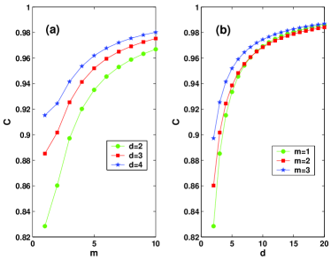
Figure 2: (Color online) The dependence relation of $C$ on $d$ and $m$.

When a vertex is generated it makes connections to all the vertices of a $(d+1)$-clique whose vertices are completely interconnected. It follows that its degree and clustering coefficient are $d+1$ and 1, respectively. In the following iterative steps, if its degree increases one by a newly created vertex connecting to it, then there must be $d$ existing neighbors of it attaching to the new vertex at the same time. Thus for a vertex of degree $k$, we have

$$C(k)={{{d(d+1)\over 2}+d(k-d-1)}\over{k(k-1)\over 2}}=\frac{2d(k-\frac{d+1}{2})}{k(k-1)}$$ (6)

where the last expression in Eq. (6) is obtained after some algebraic manipulations. From Eq. (6), one can easily see that $C(k)$ depends on degree $k$ and $d$. The asymptotic behavior for large $k$ is $C(k)\sim 1/k$, which implies that $C(k)$ is inversely proportional to the degree. Interestingly, we recover in our model the same scaling behavior of $C(k)$ found in other models DoGoMe02 ; CoFeRa04 ; RaBa03 ; No03 ; IgYa05 ; ZhRoGo05 ; AnHeAnSi05 ; DoMa05 ; ZhCoFeRo05 ; ZhYaWa05 ; ZhRoCo05 and some real-life systems RaBa03 .

Using Eq. (6), we can obtain the clustering $C$ of the networks at step $t$:

$$C=\frac{1}{N_{t}}\sum_{r=0}^{t}\frac{2d(D_{r}-\frac{d+1}{2})n_{v}(r)}{D_{r}(D_{r}-1)}$$ (7)

where the sum is the total of clustering coefficient for all vertices and $D_{r}=\frac{m(d+1)[(md)^{t-r}-1]+d^{2}-1}{d-1}$ shown by Eq. (3) is the degree of the vertices created at step $r$.

In the infinite network order limit ($N_{t}\rightarrow\infty$), Eq. (7) converges to a nonzero value. When $d=2$, for $m=1$, 2 and 3, $C$ equal to 0.8284, 0.8602 and 0.8972, respectively. When $m=2$, for $d=2$, 3 and 4, $C$ are 0.8602, 0.9017 and 0.9244, respectively. Therefore, the clustering coefficient of our networks is very high. Moreover, similarly to the degree exponent $\gamma$, clustering coefficient $C$ is determined by $d$ and $m$. Fig. 2 shows the dependence of $C$ on $d$ and $m$. From Fig. 2 (a) and (b), one can see that for any fixed $m$, $C$ increases with $d$. But the dependence relation of $C$ on $m$ (see Fig. 2 (b)) is more complex: (i) when $m\leq 2$ and $d\leq 6$, for the same $d$, $C$ increases with $m$; (ii) when $m\leq 2$ and $d>6$, for the same $d$, $C$ decreases with $m$; (iii) when $m\geq 3$, for arbitrary fixed $d$, $C$ increases with $m$. The reason for this complicated dependence relation would need further research.

IV.3 Diameter

The diameter of a network characterizes the maximum communication delay in the network and is defined as the longest shortest path between all pairs of vertices. In what follows, the notations $\lceil x\rceil$ and $\lfloor x\rfloor$ express the integers obtained by rounding $x$ to the nearest integers towards infinity and minus infinity, respectively. Now we compute the diameter of $A(d,t)$, denoted $diam(A(d,t))$ for $d\geq 2$ :

Step 0. The diameter is $1$.

Steps 1 to $\lceil\frac{d}{2}\rceil$. In this case, the diameter is 2, since any new vertex is by construction connected to a $(d+1)$-clique, and since any $(d+1)$-clique during those steps contains at least $\frac{d}{2}+2$ ($d$ even) or $\frac{d+1}{2}+1$ ($d$ odd) vertices from the initial $(d+2)$-clique $A(d,0)$ obtained after step 0. Hence, any two newly added vertices $u$ and $v$ will be connected respectively to sets $S_{u}$ and $S_{v}$, with $S_{u}\subseteq V(A(d,0))$ and $S_{v}\subseteq V(A(d,0))$, where $V(A(d,0))$ is the vertex set of $(A(d,0)$; however, since $|S_{u}|\geq\frac{d}{2}+2$ ($d$ even) and $|S_{v}|\geq\frac{d+1}{2}+1$ ($d$ odd), where $|S|$ denote thes number of elements in set $S$, we conclude that $S_{u}\cap S_{v}\neq{\O}$, and thus the diameter is 2.

Steps $\lceil\frac{d}{2}\rceil+1$ to $d+1$. In any of those steps, some newly added vertices might not share a neighbor in the original $(d+2)$-clique $A(d,0)$ obtained after step 0; however, any newly added vertex is connected to at least one vertex of the initial clique $A(d,0)$. Thus, the diameter equals to 3.

Further steps. Clearly, at each step $t\geq d+2$, the diameter always lies between a pair of vertices that have just been created at this step. We will call the newly created vertices “outer” vertices. At any step $t\geq d+2$, we note that an outer vertex cannot be connected with two or more vertices that were created during the same step $0<t^{\prime}\leq t-1$. Moreover, by construction no two vertices that were created during a given step are neighbors, thus they cannot be part of the same $(d+1)$-clique. Thus, for any step $t\geq d+2$, some outer vertices are connected with vertices that appeared at pairwise different steps. Thus, there exists an outer vertex $v_{t}$ created at step $t$, which is connected to vertices $v_{i}^{\prime}s$, $1\leq i\leq t-1$, all of which are pairwise distinct. We conclude that $v_{t}$ is necessarily connected to a vertex that was created at a step $t_{0}\leq t-d-1$. If we repeat this argument, then we obtain an upper bound on the distance from $v_{t}$ to the initial clique $A(d,0)$. Let $t=\alpha(d+1)+\beta$, where $1\leq\beta\leq d+1$. Then, we see that $v_{t}$ is at distance at most $\alpha+1$ from a vertex in $A(d,0)$. Hence any two vertices $v_{t}$ and $w_{t}$ in $A(d,t)$ lie at distance at most $2(\alpha+1)+1$; however, depending on $\beta$, this distance can be reduced by 1, since when $\beta\leq\lceil\frac{d}{2}\rceil$, we know that two vertices created at step $\beta$ share at least a neighbor in $A(d,0)$. Thus, when $1\leq p\leq\lceil\frac{d}{2}\rceil$, $diam(A(d,t))\leq 2(\alpha+1)$, while when $\lceil\frac{d}{2}\rceil+1\leq p\leq d+1$, $diam(A(d,t))\leq 2(\alpha+1)+1$. One can see that these distance bounds can be reached by pairs of outer vertices created at step $t$. More precisely, those two vertices $v_{t}$ and $w_{t}$ share the property that they are connected to $d$ vertices that appeared respectively at steps $t-1,t-2,\ldots t-d-1$.

Based on the above arguments, one can easily see that for $t>d+2$, the diameter increases by 2 every $d+1$ steps. More precisely, we have the following result, for any $d\geq 1$ and $t\geq 1$ (when $t=0$, the diameter is clearly equal to 1):

$$diam(A(d,t))=2(\lfloor\frac{t-1}{d+1}\rfloor+1)+f(d,t)$$

where $f(d,t)=0$ if $t-\lfloor\frac{t-1}{d+1}\rfloor(d+1)\leq\lceil\frac{d}{2}\rceil$, and 1 otherwise.

In the limit of large $t$, $diam(A(d,t))\sim\frac{2t}{d+1}$, while $N_{t}\sim[m(d+1)]^{t}$, thus the diameter is small and scales logarithmically with the network order.

V Conclusion and discussion

In summary, we have proposed and studied a network model, which is built in an iterative fashion. At each time step, each already existing $(d+1)$-clique, that is created at last time step, produces $m$ new vertices. The iterative process leads to a serial of networks with Apollonian networks corresponding to the particular case $m=1$. We have obtained the analytical result for degree exponent, clustering coefficient and diameter. The degree exponent and the clustering coefficient may be adjusted to various values by tuning the parameter $m$. Moreover, our networks consist of complete graphs, they may represent a variety of real-life systems such as movie actor collaboration networks, scientific collaboration networks and networks of company directors, all of which are composed of cliques AlBa02 ; DoMe03 ; SaVe04 ; Ne03 .

This research was supported by the National Natural Science Foundation of China under Grant No. 70431001.

References

- (1) R. Albert and A.-L. Barabási, Rev. Mod. Phys. 74, 47 (2002).
- (2) S. N. Dorogovtsev and J. F. F. Mendes, Evolution of Networks: From Biological Nets to the Internet and WWW (Oxford University Press, New York, 2003).
- (3) R. Pastor-Satorras and A. Vespignani, Evolution and Structure of the Internet: A Statistical Physics Approach (Cambridge University Press, Cambridge, England, 2004).
- (4) M.E.J. Newman, SIAM Review 45, 167 (2003).
- (5) A.-L. Barabási and R. Albert, Science 286, 509 (1999).
- (6) D.J. Watts and H. Strogatz, Nature (London) 393, 440 (1998).
- (7) A.-L. Barabási, E. Ravasz, and T. Vicsek, Physica A 299, 559 (2001).
- (8) F. Comellas, J. Ozón, J.G. Peters, Inf. Process. Lett. 76 (2000) 83.
- (9) F. Comellas and M. Sampels, Physica A 309 (2002) 231.
- (10) S.N. Dorogovtsev, A.V. Goltsev, and J.F.F. Mendes, Phys. Rev. E 65, 066122 (2002).
- (11) S. Jung, S. Kim, and B. Kahng, Phys. Rev. E 65, 056101 (2002).
- (12) E. Ravasz and A.-L. Barabási, Phys. Rev. E 67, 026112 (2003).
- (13) J.D. Noh, Phys. Rev. E 67, 045103 (2003).
- (14) F. Comellas, G. Fertin and A. Raspaud, Phys. Rev. E 69, 037104 (2004).
- (15) T. Zhou, B.H. Wang, P.M. Hui and K.P. Chan, e-print cond-mat/0405258.
- (16) K. Iguchi and H. Yamada, Phys. Rev. E 71, 036144 (2005).
- (17) Z.Z. Zhang, L.L Rong and C.H. Guo, e-print cond-mat/0502335 (Physica A, in press).
- (18) J.S. Andrade Jr., H.J. Herrmann, R.F.S. Andrade and L.R.da Silva, Phys. Rev. Lett. 94, 018702 (2005).
- (19) J.P.K. Doye and C.P. Massen. Phys. Rev. E 71, 016128 (2005).
- (20) Z.Z. Zhang, F. Comellas, G. Fertin and L.L. Rong, e-print cond-mat/0503316.
- (21) T. Zhou, G. Yan, and B.H. Wang, Phys. Rev. E 71, 046141 (2005).
- (22) Z.Z. Zhang, L.L Rong and F. Comellas, e-print cond-mat/0502591 (Physica A, in press).
- (23) J.P.K. Doye and C.P. Massen. J. Chem. Phys. 122, 084105 (2005).
- (24) R.F.S. Andrade and H.J. Herrmann, Phys. Rev. E 71, 056131 (2005).
- (25) P. G. Lind, J.A.C. Gallas, and H.J. Herrmann, Phys. Rev. E 70, 056207 (2004).
- (26) R.F.S. Andrade, J.G.V. Miranda, Physica A 356, 1 (2005).
- (27) R. Mahmoodi Baram, H.J. Herrmann, and N.Rivier, Phys. Rev. Lett. 92, 044301 (2004).
- (28) D.B. West, Introduction to Graph Theory (Prentice-Hall, Upper Saddle River, NJ, 2001).