Properties of 1D two-barrier quantum pump with harmonically oscillating barriers

Abstract

We study a one-dimensional quantum pump composed of two oscillating delta-functional barriers. The linear and non-linear regimes are considered. The harmonic signal applied to any or both barriers causes the stationary current. The direction and value of the current depend on the frequency, distance between barriers, value of stationary and oscillating parts of barrier potential and the phase shift between alternating voltages.

The quantum pump or a device which generate a stationary current under action of alternating voltage was a subject of numerous recent publications (for example, Moskalets03 -Lotkhov ). The quantum pump is essentially analogous to various versions of the photovoltaic effect, studied in detail from the beginning of the 1980s Bel -Iv . The difference is that the photovoltaic effect is related to the emergence of a direct current in a homogeneous macroscopic medium (the only exception is the mesoscopic photovoltaic effect), while a pump is a microscopic object. From the phenomenological point of view, the emergence of a direct current in the pump is not surprising since any asymmetric microcontact can rectify ac voltage. However, analysis of adiabatic transport in a quantum-mechanical object leads to new phenomena, such as quantization of charge transport Thouless . The quantum pump is a sample of phenomena important in living matter such as active ion transport through the cell membrane and bacterial motion (biological motors).

In the recent paper recent we have studied the one-dimensional quantum pump with two oscillating delta-like potential barriers or wells. We have found a variety of regimes of the pump operation, depending on the system parameters. In this paper we continue this study, concentrating on the non-considered cases, aimed especially at low-frequency and nonlinear operation modes of the electronic pump.

Basic Equations

We study a one-dimensional system with a potential (Fig. 1)

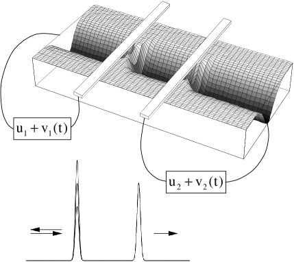
Figure 1: Up: The draft of potential of the pump. Down: One-dimensional model of the pump.

$$U(x)=(u_{1}+v_{1}(t))\delta(x+d)+(u_{2}+v_{2}(t))\delta(x-d),$$ (1)

where $v_{1}(t)=v_{1}\sin(\omega t),~{}~{}~{}v_{2}(t)=v_{2}\sin(\omega t+\varphi)$, $2d$ is the distance between $\delta$-shaped barriers (wells); quantities $u$ and $v$ are measured in units of $\hbar/md$ ($m$ is the electron mass); momentum $p$ is measured in units of $\hbar/d$; energy $E$ is measured in units of $\hbar^{2}/2md^{2}$; and frequency is measured in units of $\hbar/2md^{2}$. In the absence of an ac signal, the system has two barriers for positive values of $u_{1}$ and $u_{2}$ and two wells for negative values of these parameters. This system may be considered as a quantum wire with two narrow gates (see Figure 1) to which alternating voltages are applied. A direct current can be induced only in an asymmetric system. The specific direction in this system is determined by any of factors: the difference of static voltages $u_{1}$ and $u_{2}$, alternating voltages $v_{1}$ and $v_{2}$ or the phase shift between alternating voltages. Unlike diode system, the alternating voltages are applied to the pump by the capacitive method.

We assume that the electron gas is in equilibrium and the distribution functions are identical in the regions $x<-d$ and $x>d$. The problem is to determine the direct current induced by the ac field.

The solution to the Schrödinger equation with the potential (1) is searched in the form

$$\psi=\sum\limits_{n}e^{-i(E+n\omega)t}\times\left\{\begin{array}[]{rl}\delta_{n,0}e^{ip_{n}x/d}+r_{n}e^{-ip_{n}x/d}&x<-d,\\ a_{n}e^{ip_{n}x/d}+b_{n}e^{-ip_{n}x/d}&-d<x<d,\\ T_{n}e^{-i(p+p_{n})}e^{ip_{n}x/d}&x>d.\end{array}\right.$$ (5)

Here, $p_{n}=\sqrt{p^{2}+n\omega}$ and $p=\sqrt{E}$. The wavefunction (5) corresponds to the wave incident on the barrier from the left. (In the final formulas, we mark directions of incident waves by indices ”$\rightarrow$” and ”$\leftarrow$”). Quantities $T_{n}$ and $r_{n}$ give the amplitudes of transmission (reflection) with absorption (for $n>0$) or emission (for $n<0$) of $n$ ac field quanta, while quantity $T_{0}$ determines the amplitude of the elastic process. If the value of $p_{n}$ becomes imaginary, the waves moving away from the barriers should be treated as damped waves, so that $\mbox{Im}p_{n}>0$.

The transmission amplitudes $T_{n}$ obey the equations

$$v_{1}v_{2}g_{n-1}e^{-i\varphi}T_{n-2}^{\rightarrow}-i\left[v_{1}S_{n-1}+v_{2}V_{n}e^{-i\varphi}\right]T_{n-1}^{\rightarrow}-\bigg{[}2W_{n}+v_{1}v_{2}\Big{(}g_{n-1}e^{i\varphi}+g_{n+1}e^{-i\varphi}\Big{)}\bigg{]}T_{n}^{\rightarrow}+$$

$$i\left[v_{1}S_{n+1}+v_{2}V_{n}e^{i\varphi}\right]T_{n+1}^{\rightarrow}+v_{1}v_{2}g_{n+1}e^{i\varphi}T_{n+2}^{\rightarrow}=2ip\delta_{n,0},$$

$$v_{1}v_{2}g_{n-1}e^{-i\varphi}T_{n-2}^{\leftarrow}-i\left[v_{1}S_{n}+v_{2}V_{n-1}e^{-i\varphi}\right]T_{n-1}^{\leftarrow}-\bigg{[}2W_{n}+v_{1}v_{2}\Big{(}g_{n-1}e^{-i\varphi}+g_{n+1}e^{i\varphi}\Big{)}\bigg{]}T_{n}^{\leftarrow}+$$

$$i\left[v_{1}S_{n}+v_{2}V_{n+1}e^{i\varphi}\right]T_{n+1}^{\leftarrow}+v_{1}v_{2}g_{n+1}e^{i\varphi}T_{n+2}^{\leftarrow}=2ip\delta_{n,0}.$$ (6)

Here, $g_{n}=\sin 2p_{n}/p_{n}$,

$$S_{n}=2u_{2}g_{n}+e^{-2ip_{n}},~{}V_{n}=2u_{1}g_{n}+e^{-2ip_{n}},$$ (7)

$$W_{n}=2u_{1}u_{2}g_{n}+(u_{1}+u_{2}-ip_{n})e^{-2ip_{n}}.$$ (8)

Provided that the electrons from the right and left of the contact are in equilibrium, and they have identical chemical potentials $\mu$, the stationary current is

$$J=\frac{e}{\pi\hbar}\int dE\sum_{n}(|T_{n}^{\rightarrow}|^{2}-|T_{n}^{\leftarrow}|^{2})f(E)\theta(E+n\omega),$$ (9)

where $f(E)$ is the Fermi distribution function, and $\theta(x)$ is the Heaviside step function. The current is determined by the transmission coefficients with real $p_{n}$ only.

At a low temperature, it is convenient to differentiate the current with respect to the chemical potential $\mu$:

$${\cal G}=e\frac{\partial}{\partial\mu}J=G_{0}\sum_{n}\theta(\mu+n\omega)(|T_{n}^{\rightarrow}|^{2}-|T_{n}^{\leftarrow}|^{2})_{p=p_{F}}.$$ (10)

Here, $G_{0}=2e^{2}/h$ is the conductance quantum, $h$ is the Planck constant, and $p_{F}$ is the Fermi momentum. The resultant quantity ${\cal G}$ can be treated as a two-terminal photoconductance (the conductance for simultaneous change of chemical potentials of source and drain).

The asymptotic cases

Let us consider the limit $v_{1},v_{2}\ll u_{1},u_{2}$. The steady-state problem gives the transmission amplitude

$$T_{0}=-\frac{ip}{W_{0}}=-\frac{ip^{2}}{2u_{1}u_{2}\sin 2p+(u_{1}+u_{2}-ip)pe^{-2ip}},~{}~{}~{}~{}~{}T_{n}|_{n\neq 0}=0.$$ (11)

The scattering amplitude vanishes for $p\to 0$ and experiences oscillations with a period $\delta p=\pi/2$. For large values of $u_{l,2}$, quantity $T_{0}$ has poles in the vicinity of points $p=\pi n/2$.

In the zeroth order of perturbation theory, the direct and reverse transmission coefficients coincide; consequently, the current vanishes. The current appears only in the second order of perturbation theory. Second-order corrections to the current come only from quantities $T_{0}$, $T_{1}$, and $T_{-1}$. Expanding in the ac signal, we obtain

$${\cal G}=G_{0}\frac{p^{2}}{4|W_{0}|^{2}}\Bigg{\{}v_{1}^{2}\left(\frac{|S_{0}|^{2}-|S_{-1}|^{2}}{|W_{-1}|^{2}}\theta(\mu-\omega)+\frac{|S_{0}|^{2}-|S_{1}|^{2}}{|W_{1}|^{2}}\right)-$$

$$v_{2}^{2}\left(\frac{|V_{0}|^{2}-|V_{-1}|^{2}}{|W_{-1}|^{2}}\theta(\mu-\omega)+\frac{|V_{0}|^{2}-|V_{1}|^{2}}{|W_{1}|^{2}}\right)+$$ (12)

$$2v_{1}v_{2}~{}\mbox{Re}\left[\frac{S_{0}V_{-1}^{*}-S_{-1}V_{0}^{*}}{|W_{-1}|^{2}}e^{-i\varphi}\theta(\mu-\omega)+\frac{S_{0}V_{1}^{*}-S_{1}V_{0}^{*}}{{|W_{1}|^{2}}}e^{i\varphi}\right]+$$

$$4v_{1}v_{2}\sin\varphi~{}\mbox{Im}\left[\frac{S_{0}V_{0}-S_{-1}V_{-1}}{W_{0}W_{-1}}-\frac{S_{0}V_{0}-S_{1}V_{1}}{W_{0}W_{1}}+2\frac{g_{-1}-g_{1}}{W_{0}}\right]\Bigg{\}}_{p=p_{F}}.$$

In the particular case when $u_{1}=u_{2}$, the functions $S_{n}$ and $V_{n}$ coincide, and the expression (The asymptotic cases) obtains the form

$${\cal G}=G_{0}\frac{p^{2}}{4|W_{0}|^{2}}\Bigg{\{}\left(v_{1}^{2}-v_{2}^{2}\right)\left(\frac{|S_{0}|^{2}-|S_{-1}|^{2}}{|W_{-1}|^{2}}\theta(\mu-\omega)+\frac{|S_{0}|^{2}-|S_{1}|^{2}}{|W_{1}|^{2}}\right)+$$

$$4v_{1}v_{2}\sin\varphi~{}\mbox{Im}\left[\frac{S_{0}S_{-1}^{*}}{|W_{-1}|^{2}}\theta(\mu-\omega)-\frac{S_{0}S_{1}^{*}}{{|W_{1}|^{2}}}+\frac{S_{0}^{2}-1}{W_{0}}\left(\frac{1}{W_{-1}}-\frac{1}{W_{1}}\right)\right]\Bigg{\}}_{p=p_{F}}.$$ (13)

The current is determined by the corrections $T_{\pm 1}$ associated with real emission (absorption) of a single photon. In addition, a correction to $T_{0}$ associated with the effect of a virtual single-photon process on the nonradiative channel also exists. Apart from the squares of ac signals $v_{1}$ and $v_{2}$, the result for the regime $u_{1}=u_{2}$ contains a bilinear combination; consequently, it is insufficient to consider the response only at one of the signals. The latter contribution is sensitive to the relative phase of the signals.

In the case of the large $u_{1}$ and $u_{2}$ compared with the Fermi momentum, the expression (The asymptotic cases) yields

$${\cal G}=G_{0}\frac{p^{2}v_{1}^{2}\sin\varphi}{8u_{1}^{7}g_{0}}\left\{\frac{\left(3p_{-1}-p\right)\theta(\mu-\omega)}{g_{-1}}-\frac{3p_{1}-p}{g_{1}}\right\}_{p=p_{F}}\stackrel{{\scriptstyle\small\omega\to 0}}{{\longrightarrow}}G_{0}\frac{\omega p_{F}^{3}v_{1}^{2}\sin\varphi\left[4p_{F}\cot 2p_{F}-5\right]}{8u_{1}^{7}\sin^{2}2p_{F}}.$$ (14)

If $u_{1}=u_{2}=0$,

$${\cal G}=G_{0}v_{1}v_{2}\sin\varphi\left\{\frac{\sin 2(p-p_{-1})}{p_{-1}^{2}}\theta(\mu-\omega)+\frac{\sin 2(p_{1}-p)}{p_{1}^{2}}\right.$$

$$\left.+\frac{2\sin 2p}{p}\left(\frac{\cos 2p_{-1}}{p_{-1}}\theta(\mu-\omega)-\frac{\cos 2p_{1}}{p_{1}}\right)\right\}_{p=p_{F}}.$$ (15)

The expression (The asymptotic cases) tends to infinity at the single photon emission threshold. This singularity can be explained by the resonance with the state of an electron with zero energy: such an ”immobile” state can be interpreted as a bound state.

In addition to the above-mentioned oscillations with period $\delta p=\pi/2$, the transmission amplitude experiences oscillations with periods $\delta p_{\pm 1}=\pi/2$. It can be seen from expression (The asymptotic cases) that the extrema in the dependence of the current on $p$ are located in the vicinity of the points corresponding to the minima of functions $W_{0}$ and $W_{\pm 1}$ and are connected with the elastic process as well as with the process involving the absorption or emission of a field quantum. For $v_{2}=0$($v_{1}=0$), the expression for the current contains only one term proportional to $v_{1}^{2}$($v_{2}^{2}$).

For $u_{1},u_{2}\gg p$ the oscillations are transformed into sharp peaks corresponding to the transmission resonances. For $p\sim 1$, the transmission amplitude has a characteristic scale of $p\sim u_{1},u_{2}$. The corresponding structure for small values of $u_{1}$ and $u_{2}$ can be treated as a resonance at zero energy. For negative values of $u_{1}$ and $u_{2}$, resonance at bound states exist (at one or two such states depending on the distance between the wells).

Numerical results.

The Figure 2 shows the dependence of the stationary current $J$ on the Fermi momentum in a symmetric structure with two $\delta$-wells ($|u_{1}|=|u_{2}|\gg v_{1}=v_{2},~{}\varphi=\pi/2$). The current oscillate with the Fermi momentum with the period $\pi/2$. These oscillations are related to the resonance at quasi-stationary states between the wells. The threshold singularity at $p_{F}=5$ is associated with zero-energy one-photon resonance.

Figure 2: The dependence of the stationary current $J$ (in units $e\hbar/2\pi md^{2}$) on the Fermi momentum in a symmetric structure $u_{1}=u_{2}=-1,~{}v_{1}=v_{2}=0.1,~{}\omega=25,~{}\varphi=\pi/2$.

The Figure 3 demonstrates the dependence of the quantity $\cal G$ on the Fermi momentum in the symmetric structure with two identical $\delta$-wells and - $\delta$-barriers. These cases differs by the sign of the quantity $\cal G$ and by the small relative shift of the position of the resonance singularities. Really, within the limits of large $u_{1}=u_{2}$ at $\omega\to 0$ the quantity ${\cal G}\propto u_{1}^{-7}$ (14), i.e. is odd function of amplitude $u_{1}$ and accordingly, changes the sign with the changing of the $u_{1}$ sign. The shift of the position of the resonance singularities is connected with the difference of quasi-stationary energy levels in these cases.

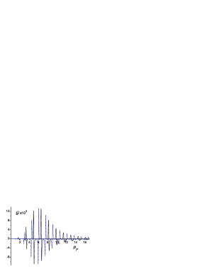
Figure 3: The dependence of $\cal G$ on the Fermi momentum in a symmetric structure $u_{1}=u_{2}=\pm 1,~{}v_{1}=v_{2}=0.1,~{}\omega=1,~{}\varphi=\pi/2$. The solid and dashed curves corresponds to $u_{1}=1$ and $u_{1}=-1$, accordingly.

The Figure 4 depicts $\cal G$ as a function of Fermi momentum for two values of the phase $\varphi$ in the symmetric device. It demonstrates that $\cal G$ is phase-sensitive for small $p_{F}$ up to $p_{F}\sim 5$. The change of phase modifies the curve, in particular visibly shifts the first deep. For large $p_{F}>5$ the curves correspond to the perturbative expression (The asymptotic cases).

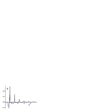
Figure 4: The dependence of $\cal G$ on the Fermi momentum $u_{1}=u_{2}=v_{1}=v_{2}=5,~{}\omega=0.1$ for $\varphi=\pi/2$ (solid curve) and $\varphi=\pi/3$ (dashed curve).

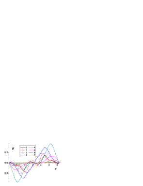
Figure 5: The dependence of $\cal G$ on the phase shift $\varphi$ in a symmetric structure $\omega=1,~{}p_{F}=2,~{}v_{1}=v_{2}=5,~{}u_{1}=u_{2}=0,1,2,3,4,5,6,7.$

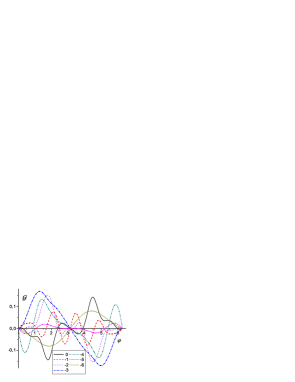
Figure 6: The dependence of $\cal G$ on the phase shift $\varphi$ in a symmetric structure $\omega=1,~{}p_{F}=2,~{}v_{1}=v_{2}=5,~{}u_{1}=u_{2}=0,-1,-2,-3,-4,-5,-6.$

The Figures 5 and 6 show the evolution of the function $\cal G(\varphi)$ in the symmetric device with two barriers (5) or two wells (6) with the value of alternating signal at a fixed $p_{F}=2$. The case of large $u_{1,2}\gg v_{1,2}$ corresponds to the perturbative expression (The asymptotic cases). This explains the approximative sinusoidal dependence of $\cal{G}$ on the phase for $|u_{1,2}|>5$. For relatively small Fermi momenta $p_{F}<v_{1,2}$, and if also $u_{1,2}\leq v_{1,2}$, the harmonic (sinus-like) dependence of $\cal G(\varphi)$ is superimposed on the short-period ($\pi/2$) oscillations conditioned by the resonance in 4th order of the perturbation theory.

The Figure 7 demonstrates the dependence of $\cal G$ on the frequency of the alternating signal in the low-frequency limit. The linear dependence of $\cal G$ in the low-frequency limit agrees with (14). The threshold singularity at $\omega=0.5$ is related to zero-energy one-photon resonance.

Figure 7: The dependence of $\cal G$ on the frequency $u_{1}=1,~{}u_{2}=3,~{}v_{1}=v_{2}=0.1,~{}\varphi=\pi/2,~{}p_{F}=0.71$.

The Figure 8 depicts $\cal{G}$ for strong low-frequency alternating voltages. The resonance at $p_{F}=\pi/2$, which presents in the low-signal regime (see the curve a) obtains the photon repetitions. They overlap composing damped (with the number of photons) oscillations. The oscillations rarefy with the increase of the frequency.

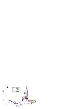
Figure 8: The dependence of $\cal G$ on the Fermi momentum for different small frequencies (shown in the figure); $u_{1}=u_{2}=v_{1}=v_{2}=5,~{}\varphi=\pi/4$. The curve a) represents low- signal result for $u_{1}=u_{2}=5,~{}~{}v_{1}=v_{2}=1,~{}\varphi=\pi/4,~{}\omega=0.1$.

Conclusions

The problem of stationary current induced by harmonic signals applied via two gates to one-dimensional system was studied. The considered system is described by the simplified double delta-functional time-dependent barriers. The regimes of weak and strong external voltage were considered. The current experiences oscillations as a function of chemical potential. These oscillations turn into interference resonances if the stationary barriers or the alternating voltages are strong enough. The resonances have many-photon nature. The current depends on the phase shift between gates.

The work was supported by grants of RFBR Nos. 05-02-16939 and 04-02-16398, Program for support of scientific schools of the Russian Federation No. 593.2003.2 and the Dynasty Foundation.

References

• (1) M. Moskalets and M. Büttiker, Phys. Rev. B 68 161311(R) (2003).
• (2) J.E. Avron, A. Elgart, G.M. Graf, and L. Sadun, Phys. Rev. B 62, R10618 (2000).
• (3) J.E. Avron, A. Elgart, G.M. Graf, and L. Sadun, Phys. Rev. Lett. 87, 236601 (2001).
• (4) O. Entin-Wohlman and Amnon Aharony, Phys. Rev. B 65, 195411 (2002).
• (5) D. Cohen, Phys. Rev. B 68, 155303 (2003).
• (6) Huan-Qiang Zhou, Sam Young Cho, and Ross H. McKenzie, Phys. Rev. Lett. 91, 186803 (2003).
• (7) M. Moskalets and M. Büttiker, Phys. Rev. B 66, 205320 (2002).
• (8) F. Rengozi, T. Brandes, Phys. Rev. B 64, 2045301 (2001).
• (9) Shi-Liang Zhu and Z. D. Wang, Phys. Rev. B 65, 155313 (2002).
• (10) C.S. Tang, C.S. Chu, Solid State Commun., 120 353 (2001).
• (11) Baigeng Wang, Jian Wang, and Hong Guo, Phys. Rev. B 68, 155326 (2003).
• (12) M. Switkes, C.M. Marcus, K. Campman, and A.C. Gossard, Science 283 1905 (1999).
• (13) T. Altebaeumer, H Ahmed, Japanese Journal of Applied Physics, part I, 41, Iss 4B, 2694 (2002).
• (14) Y. Ono, Y Takahashi, Applied Physics Lett, 82, 1221(2003).
• (15) S.V. Lotkhov, S.A. Bogoslovsky, A.B. Zorin, J. Niemeyer, Applied Physivs Lett., 78, 946 (2001).
• (16) V.I. Belinicher and B.I. Sturman, Usp. Fiz. Nauk 130, 415 (1980)[Sov. Phys. Usp. 23, 199 (1980)].
• (17) M.D. Blokh, L.I. Magarill, and M.V. Entin, Fiz. Tekh. Poluprovodn. (Leningrad) 12, 249 (1978)[Sov. Phys. Semicond. 12, 143 (1978)].
• (18) E.M. Baskin, L.I. Magarill, and M.V. Entin, Fiz. Tverd. Tela (Leningrad) 20, 2432 (1978)[Sov. Phys. Solid State 20, 1403 (1978)].
• (19) E.L. Ivchenko and G.E. Pikus, Pis’ma Zh. Eksp. Teor. Fiz. 27, 640 (1978)[JETP Lett. 27, 604 (1978)].
• (20) D.J. Thouless, Phys. Rev. B 27, 6083 (1983).
• (21) L.S. Braginskii, M.M. Makhmudian, and M.V. Entin, Zh. Eksp. Teor. Fiz. 127, 1046 (2005)[JETP 100, 920 (2005)].
• (22) R.D. Astumian, Phys. Rev. Lett. 91, 118102 (2003).
• (23) S.W. Kim, Phys. Rev. B 66, 235304 (2002).