Towards a fully automated computation of RG-functions for the $3$-$d$ $O(N)$ vector model:
Parametrizing amplitudes

Abstract

Within the framework of field-theoretical description of second-order phase transitions via the $3$-dimensional $O(N)$ vector model, accurate predictions for critical exponents can be obtained from (resummation of) the perturbative series of Renormalization-Group functions, which are in turn derived —following Parisi’s approach— from the expansions of appropriate field correlators evaluated at zero external momenta.

Such a technique was fully exploited $30$ years ago in two seminal works of Baker, Nickel, Green and Meiron ([1]-[2]), which lead to the knowledge of the $\beta$-function up to the $6$-loop level; they succeeded in obtaining a precise numerical evaluation of all needed Feynman amplitudes in momentum space by lowering the dimensionalities of each integration with a cleverly arranged set of computational simplifications. In fact, extending this computation is not straightforward, due both to the factorial proliferation of relevant diagrams and the increasing dimensionality of their associated integrals; in any case, this task can be reasonably carried on only in the framework of an automated environment.

On the road towards the creation of such an environment, we here show how a strategy closely inspired by that of Nickel and coworkers can be stated in algorithmic form, and successfully implemented on the computer. As an application, we plot the minimized distributions of residual integrations for the sets of diagrams needed to obtain RG-functions to the full $7$-loop level; they represent a good evaluation of the computational effort which will be required to improve the currently available estimates of critical exponents.

¹, ²

• Preprint HU-EP-05/39, SFB/CPP-05-64, SPhT-T05/128

1 Motivation

A great achievement of the Renormalization-Group (RG) approach to critical phenomena (introduced in [3], [4], [5], [6], [7], [8]) is the realization that the universal behavior of many different physical systems can be explained by the existence of a common large-distance fixed point —or infrared, or IR fixed point— of RG-equations; these equations describe the evolution of the effective Hamiltonians for such systems when the short-distance degrees of freedom —also called ultraviolet, or UV— are increasingly summed up. In particular, it turns out from this idea that a quantitative description of physical universal quantites such as critical exponents and critical amplitudes can be obtained by considering the RG-evolution of a euclidean quantum field theory appropriately chosen to stay in the same universality class of the systems to be described. In this perspective, second-order phase transitions of systems with $N$ phenomenological scalar components in the sense of Landau theory can be obtained by studying the IR fixed point(s) of the RG-equations for quantum field theories of $N$ interacting scalar fields. In the case of $O(N)$-symmetric interactions of $\left(\phi^{2}\right)^{2}$ type, the IR fixed point is known as Wilson-Fisher fixed point (see [9]).

Following this line of thought, during the Cargese summer school in 1973, [10], Parisi made the seminal observation that a quantitative description of the Wilson-Fisher fixed point can be obtained by analyzing the Callan-Symanzik RG-equations for a system of $3$-dimensional massive scalar bosons with an $O(N)$-invariant interaction of $\left(\phi^{2}\right)^{2}$ type, the so-called $O(N)$ vector model (first published notes of this idea can be found in [11]). Such a theory is a super-renormalizable one, i.e. the number of one-particle irreducible (OPI) diagrams with new primitive divergences is finite, and renormalization process is easier if compared to that required by other renormalizable theories.

A price to pay for the simplicity of Parisi’s approach is the fact that the value of the coupling is nonperturbatively large at the fixed point; thus, the perturbative series obtained in this framework have to be resummed by means of a suitable method (the one usually chosen being the so-called Borel summation). We do not dive here into the details of these resummation techniques; we only mention that for this field-theoretical model it has been rigorously proved in [12] that resummed perturbative series converge when their order increases; thus, the precision of the estimates obtained within Parisi’s approach is only limited by our practical ability in generating and parametrizing the necessary amplitudes up to the desired order, and by the precision we can reach when computing the high-dimensional integrals in terms of which amplitudes are expressed. As an additional remark, one should bear in mind that, to avoid instabilities in the resummation process at a given perturbative order, the numerical precision of each term of the series should be greater than that desired for the final result, and greater than that of subsequent terms as well.

The panorama of results in the computation of RG-functions for the $3$-dimensional $O(N)$ vector model is dominated by the work of B. G. Nickel and collaborators. In 1976-1978 —see [1] and [2]—, making use of a large and cleverly-arranged set of remarkable computational simplifications partially described in [20], Baker, Nickel, Green and Meiron were able to push the calculation from the $2$-loop- (see [10] and [21]) up to the $6$-loop- level. (See also [22] for a compilation of diagrams, weights and associated amplitude values; [23] is an application of the same type of data to a different context.) In 1991 Murray and Nickel [24] completed the evaluation of an improved estimate of the anomalous dimensions $\eta$ and $\eta_{2}$ including partial $7$-loop results, but the full $7$-loop computation of RG $\beta$-function and critical exponents is still an open problem. It should be noticed that from a technical point of view —and in particular when taking into account the lack of available computer power at the time— the $6$-loop calculation is already an outstanding masterpiece in its own right: in fact, it requires the high-precision numerical evaluation (with $8$-$10$ significant digits) of a thousand diagrams, which were apparently parametrized by hand as integrals with up to $6$ residual dimensions, in the careful attempt of finding the most advantageous representation for each amplitude.

As a matter of fact, a very conspicuous body of literature relies on [2], [24] and the compilation [22] for the calculation of critical exponents as well as of other quantities (see for example [25] and [26], [27], [28]). However, at least in our knowledge, no other group has been able to reproduce these computations independently so far: this fact has been our main motivation for resuming the problem, in the hope of being able to verify —and possibly extend— the results available at present.

The high number of diagrams which must be evaluated to complete the calculation of the $7$th loop ($\sim 4000$, see section 3.2.2) makes it immediately clear that the only realistic hope to push forward our knowledge relies on finding a way of automating computations by means of computer techniques; the goal of this paper is then to perform the first steps towards the build-up of such an automated environment, both for generation and parametrization of all needed Feynman amplitudes. Article structure is as follows:

• In section 2 we introduce all relevant information about the $3$-dimensional $O(N)$ vector model, together with the renormalization scheme and the RG-equations our computations are based on

• In section 3 we briefly discuss how to generate all needed Feynman diagrams, together with their combinatorial and $O(N)$ factors; after that, we analyze in great detail the set of analytic tricks which make possible an efficient parametrization of the associated amplitudes. A number of practical examples is given

• In section 4 we provide a precise algorithmic formulation for each of the tasks required to actually find the set of optimal parametrizations at some given perturbative level

• In section 5 we describe our computer implementation of such techniques, and the results we obtained so far. A critical discussion follows about how the set of chosen simplifications influences both the complexity of the parametrization code and the minimality of the resulting set of parametrizations.

2 The $3$-dimensional $O(N)$ vector model

2.1 Generalities

The $3$-dimensional $O(N)$ vector model is described by a classical (bare) action which is invariant under a transformation of the scalar fields $\phi_{\scriptscriptstyle{\mathrm{B}}}^{i}$ ($i=1,\,\ldots\,,\,N$) according to a fundamental representation of $O(N)$:

$$S_{\scriptscriptstyle{\mathrm{B}}}(\phi_{\scriptscriptstyle{\mathrm{B}}}):=\int d^{3}x\left(\frac{1}{2}(\nabla\phi_{\scriptscriptstyle{\mathrm{B}}})^{2}+{m^{2}_{\scriptscriptstyle{\mathrm{B}}}\over 2}\phi_{\scriptscriptstyle{\mathrm{B}}}^{2}+{\lambda_{\scriptscriptstyle{\mathrm{B}}}\over 4!}(\phi_{\scriptscriptstyle{\mathrm{B}}}^{2})^{2}\right).$$ (1)

The quantization of the model is obtained via functional integration, by considering the (bare) generating functional,

$$Z_{\scriptscriptstyle{\mathrm{B}}}(J_{\scriptscriptstyle{\mathrm{B}}}):=\int[d\phi_{\scriptscriptstyle{\mathrm{B}}}]\exp\left(-S_{\scriptscriptstyle{\mathrm{B}}}(\phi_{\scriptscriptstyle{\mathrm{B}}})+\int J_{\scriptscriptstyle{\mathrm{B}}}\phi_{\scriptscriptstyle{\mathrm{B}}}\right).$$ (2)

An appropriate regularization —parametrized by some ultraviolet cutoff denoted with $\Lambda$— is necessary to give meaning to functional integration. We assume that such a regularization exists, but to maintain generality and simplicity of notations we will not show its details here. As well known, perturbation theory for the bare model is plagued by ultraviolet divergences in the limit $\Lambda\to\infty$, and must be complemented by renormalization; that amounts to a reparametrization of bare (ultraviolet) quantities in terms of renormalized (infrared) ones. In this section we content ourselves with briefly recalling only some essential points about the renormalization of the $O(N)$ vector model; all other necessary definitions and some additional technical details about it, including a derivation of Callan-Symanzik equations in a generic massive renormalization scheme, are reported for reference in A.

Applying standard power counting techniques to Feynman diagrams obtained from the perturbative expansion of the $O(N)$ vector model, it is easy to compute the superficial degree of divergence $\omega$ for the Feynman amplitude ${\mathcal{A}_{\mathfrak{D}}}$ associated to a connected one-particle irreducible, or OPI, diagram ${\mathfrak{D}}$ with ${E}$ external legs, ${V_{2}}$ insertions of operator $\int\phi^{2}$ and ${V_{4}}$ vertices with four legs. The obtained expression reads

$$\omega=3-\frac{{E}}{2}-{V_{4}}-2{V_{2}};$$ (3)

roughly speaking, $\omega$ parametrizes the behaviour of the amplitude in the limit $\Lambda\to\infty$, where ${\mathcal{A}_{\mathfrak{D}}}\sim\Lambda^{\omega}$ (see [29] for a more rigorous definition). It turns out from (3) that the model is super-renormalizable, i.e. it has only a finite number of superficially divergent amplitudes. When restricting to the conditions ${E}>0$ —as it is always the case in this article— and ${{L}}>0$, amplitudes must satisfy ${E}=2$, ${V_{2}}=0$ and ${V_{4}}=1,2$ to have $\omega\geq 0$ and to possibly be superficially divergent; these constraints are verified in our model only by the three graphs listed below:

$$\begin{array}[]{ccc}\includegraphics[width=65.04034pt]{tadpole.eps},&\includegraphics[width=65.04034pt]{doubleTadpole.eps},&\includegraphics[width=65.04034pt]{sunset.eps},\end{array}$$

which we will call in the rest of this article —from left to right— “tadpole”, “cactus”, and “sunset”, respectively. It should also be noticed that these divergent graphs require a mass renormalization, but no divergent contribution affects the derivative of the two-point function w.r.t. $p^{2}$, i.e. wave-function renormalization is not needed to make the theory finite.

2.2 Intermediate scheme

From a practical point of view, the most effective way of proceeding is to first choose an intermediate renormalization scheme, with the goal of making the theory finite and the calculations as simple as possible; only after that —in the end— one will switch to the final renormalization scheme presented in section 2.3. More in detail, our own intermediate scheme (labeled with suffix ${\scriptscriptstyle{\mathrm{I}}}$ and referred to as “I-scheme”) is defined by the following conditions:

$$\phi_{\scriptscriptstyle{\mathrm{B}}}=\phi_{\scriptscriptstyle{\mathrm{I}}}$$ (5)

$$\phi_{\scriptscriptstyle{\mathrm{B}}}^{2}=\left[\phi^{2}\right]_{\scriptscriptstyle{\mathrm{I}}}$$ (6)

$$\lambda_{\scriptscriptstyle{\mathrm{B}}}=m_{\scriptscriptstyle{\mathrm{I}}}g_{\scriptscriptstyle{\mathrm{I}}}$$ (7)

$$m_{\scriptscriptstyle{\mathrm{B}}}^{2}=m^{2}_{\scriptscriptstyle{\mathrm{I}}}+\delta m^{2}_{\scriptscriptstyle{\mathrm{I}}};$$ (8)

the mass counterterm is in turn defined as:

$$\delta m^{2}_{\scriptscriptstyle{\mathrm{I}}}:=-\left(\includegraphics[width=43.36464pt]{tadpole.eps}+\left.\begin{minipage}[c]{43.36464pt} \includegraphics[width=433.62pt]{sunset.eps} \end{minipage}\right|_{\boldsymbol{p}=\boldsymbol{0}}\right).$$ (9)

From such definition it follows that in the I-scheme the renormalized contribution of the “tadpole” fully vanishes, while the renormalized contribution of the “sunset” vanishes at $\boldsymbol{p}=\boldsymbol{0}$. As a consequence, the renormalized contribution of the “cactus” diagram vanishes too, because the “cactus” amplitude factors in terms of a “tadpole” amplitude times a finite term. (Please remark that in (9) we did not write the explicit form of $\delta m^{2}_{\scriptscriptstyle{\mathrm{I}}}$, being it dependent on the choice of regularization.)

As a first important property of our intermediate scheme, an inspection of counterterms listed in (9) readily shows the absence of potential overlapping divergent (sub)graphs. Thus, the procedure of renormalization amounts in the I-scheme to mechanically replacing all the instances of divergent graphs with their renormalized counterparts when they occur as subgraphs embedded in larger graphs; in practice, all needed operations can be performed by just putting “tadpole” subdiagrams to zero, and by replacing all occurrencies of the “sunset” with a renormalized version, obtained from the original one by subtracting the value of the diagram in zero.

This trivialization of renormalization is a fondamental assumption in the automated framework presented in this paper, and its consistent practical advantages will be silently used everywhere throughout all our parametrization algorithms; it should be noticed that this property —which is far from being always guaranteed— depends in general both on the structure of primitive divergences of the model considered and on the type of subtractions that are performed in a given renormalization scheme.

Another remarkable property of the I-scheme is that $\phi_{\scriptscriptstyle{\mathrm{I}}}$ and $[\phi^{2}]_{\scriptscriptstyle{\mathrm{I}}}$ do not renormalize, i.e. ${Z_{\phi,{\scriptscriptstyle{\mathrm{I}}}}}={Z_{\phi^{2},{\scriptscriptstyle{\mathrm{I}}}}^{\phi^{2}}}=1;$ this fact implies the vanishing of corresponding anomalous dimensions

$$\eta_{\scriptscriptstyle{\mathrm{I}}}(g_{\scriptscriptstyle{\mathrm{I}}})=\eta_{2{\scriptscriptstyle{\mathrm{I}}}}(g_{\scriptscriptstyle{\mathrm{I}}})=0$$ (10)

(see A for general definitions of $Z$-terms and anomalous dimensions). Triviality of $Z$-terms implies in turn the following set of relations, valid for ${E}>0$:

$$\Gamma_{{\scriptscriptstyle{\mathrm{I}}}}^{({E},{V_{2}})}\!\left({\underline{\boldsymbol{p}}};{\underline{\boldsymbol{q}}};m^{2}_{\scriptscriptstyle{\mathrm{I}}},g_{\scriptscriptstyle{\mathrm{I}}}\right)=\Gamma_{\scriptscriptstyle{\mathrm{B}}}^{({E},{V_{2}})}\!\left({\underline{\boldsymbol{p}}};{\underline{\boldsymbol{q}}};m^{2}_{\scriptscriptstyle{\mathrm{B}}}=m^{2}_{\scriptscriptstyle{\mathrm{I}}}+\delta m^{2}_{\scriptscriptstyle{\mathrm{I}}},\lambda_{\scriptscriptstyle{\mathrm{B}}}=m_{\scriptscriptstyle{\mathrm{I}}}g_{\scriptscriptstyle{\mathrm{I}}}\right).$$ (11)

Remark in the equation above the use of ${\underline{\boldsymbol{p}}}$, ${\underline{\boldsymbol{q}}}$ to denote respectively the collections $(\boldsymbol{p}_{1},\,\ldots\,,\,\boldsymbol{p}_{E})$, $(\boldsymbol{q}_{1},\,\ldots\,,\,\boldsymbol{q}_{V_{2}})$; please consult A for more details on our notations.

The Callan-Symanzik operator in the I-scheme, $\mathcal{D}_{\scriptscriptstyle{\mathrm{I}}}$, is defined by specializing to such a scheme the general definition in (100):

$$\mathcal{D}_{\scriptscriptstyle{\mathrm{I}}}:=\left.m_{\scriptscriptstyle{\mathrm{I}}}\frac{d}{dm_{\scriptscriptstyle{\mathrm{I}}}}\right|_{\lambda_{\scriptscriptstyle{\mathrm{B}}},\Lambda}.$$ (12)

Applying $\mathcal{D}_{\scriptscriptstyle{\mathrm{I}}}$ to both sides of (7) the expression for the $\beta$-function is easily derived:

$$\beta_{\scriptscriptstyle{\mathrm{I}}}(g_{\scriptscriptstyle{\mathrm{I}}})=\mathcal{D}_{\scriptscriptstyle{\mathrm{I}}}[g_{\scriptscriptstyle{\mathrm{I}}}]=-g_{\scriptscriptstyle{\mathrm{I}}}.$$ (13)

The exact Callan-Symanzik equation in the I-scheme (assuming ${E}>0$) then reads:

$$\left[m_{\scriptscriptstyle{\mathrm{I}}}\frac{\partial}{\partial m_{\scriptscriptstyle{\mathrm{I}}}}-g_{\scriptscriptstyle{\mathrm{I}}}\frac{\partial}{\partial g_{\scriptscriptstyle{\mathrm{I}}}}\right]\Gamma_{{\scriptscriptstyle{\mathrm{I}}}}^{({E},{V_{2}})}\!\left({\underline{\boldsymbol{p}}};{\underline{\boldsymbol{q}}}\right)=m_{\scriptscriptstyle{\mathrm{I}}}^{2}\sigma_{\scriptscriptstyle{\mathrm{I}}}(g_{\scriptscriptstyle{\mathrm{I}}})\;\Gamma_{{\scriptscriptstyle{\mathrm{I}}}}^{({E},{V_{2}}+1)}\!\left({\underline{\boldsymbol{p}}};{\underline{\boldsymbol{q}}},\boldsymbol{q}_{{V_{2}}+1}=0\right)$$ (14)

where the $\sigma$-function is obtained by applying its definition (107) to (8), (9):

$$\sigma_{\scriptscriptstyle{\mathrm{I}}}\left(g_{\scriptscriptstyle{\mathrm{I}}}\right)=2+\frac{N+2}{24\pi}g_{\scriptscriptstyle{\mathrm{I}}}-\frac{N+2}{288\pi^{2}}g_{\scriptscriptstyle{\mathrm{I}}}^{2}.$$ (15)

(It should be noticed that, regardeless of the dependence of $\delta m^{2}_{\scriptscriptstyle{\mathrm{I}}}$ on the cutoff $\Lambda$, the expression of $\sigma_{\scriptscriptstyle{\mathrm{I}}}\left(g_{\scriptscriptstyle{\mathrm{I}}}\right)$ does not depend on the choice of regularization in the limit $\Lambda\to\infty$, as it should be for all RG-functions in a well-behaved renormalization scheme.)

In spite of their apparent simplicity, Callan-Symanzik equations in the I-scheme are not at all trivial! For instance, specializing to $({E},{V_{2}})=(2,0)$ at $\boldsymbol{p}=\boldsymbol{0}$ and introducing the rescaled function

$$\widehat{\Gamma_{\scriptscriptstyle{\mathrm{I}}}^{(2,0)}}\!\left(g_{\scriptscriptstyle{\mathrm{I}}}\right):=\Gamma_{\scriptscriptstyle{\mathrm{I}}}^{(2,0)}\!\left({\underline{\boldsymbol{0}}};m_{\scriptscriptstyle{\mathrm{I}}},g_{\scriptscriptstyle{\mathrm{I}}}\right)/m^{2}_{\scriptscriptstyle{\mathrm{I}}}$$ (16)

we obtain the exact relation

$$\left[2-g_{\scriptscriptstyle{\mathrm{I}}}\frac{\partial}{\partial g_{\scriptscriptstyle{\mathrm{I}}}}\right]\widehat{\Gamma_{\scriptscriptstyle{\mathrm{I}}}^{(2,0)}}\!\left(g_{\scriptscriptstyle{\mathrm{I}}}\right)=\sigma_{\scriptscriptstyle{\mathrm{I}}}(g_{\scriptscriptstyle{\mathrm{I}}})\;\Gamma_{{\scriptscriptstyle{\mathrm{I}}}}^{(2,1)}\!\left({\underline{\boldsymbol{0}}};\boldsymbol{q}=\boldsymbol{0};g_{\scriptscriptstyle{\mathrm{I}}}\right)$$ (17)

which can be used to link two quantities involved in the computation of RG-functions, see discussion below.

Before closing this section some comments are in order to motivate our own choice of the I-scheme as intermediate renormalization scheme.

It should be clear from the considerations presented above —and in particular from the definition of mass counterterm in (9)— that the main peculiarity of the I-scheme is that a minimal number of counterterms is introduced. This property results in a minimal amount of renormalized diagrams and turns out to be invaluable to simplify the automatization of the parametrization process, expecially in view of cost optimization — see section 4. This simplicity, together with the desire of testing existing results in the most independent way as possible, mainly motivates our choice of the I-scheme, which is in fact quite different from the one employed in [22].

The price we have to pay for this conceptual simplification is that in this scheme we may have more diagrams to evaluate than in other possible schemes; in our case, for example, the renormalized high-order contributions to $\Gamma^{\left(2,0\right)}_{\scriptscriptstyle{\mathrm{I}}}(\boldsymbol{p}=\boldsymbol{0})$ are not trivially vanishing — apart from the “sunset” graph and all graphs with “tadpole” insertion(s). In particular, one relevant difference w.r.t. the scheme used in [22] is that in our I-scheme $2$-point connected OPI (sub-)graphs with external lines connecting to the same vertex (which we refer to as to generalized tadpoles) give in general rise to non-zero contributions, and must thus be evaluated. However, this complication is not a dramatic problem for at least two reasons:

1. the expression of $\Gamma^{\left(2,0\right)}_{\scriptscriptstyle{\mathrm{I}}}(\boldsymbol{p}=\boldsymbol{0})$ can actually be obtained from that of $\Gamma^{\left(2,1\right)}_{\scriptscriptstyle{\mathrm{I}}}(\boldsymbol{p}=\boldsymbol{q}=\boldsymbol{0})$ by use of the exact Callan-Symanzik equation in I-scheme, (17)

2. anticipating section 2.3, we remark that in addition to that of $\Gamma^{\left(2,0\right)}_{\scriptscriptstyle{\mathrm{I}}}(\boldsymbol{p}=\boldsymbol{0})$ also the expressions for $\Gamma^{\left(4,0\right)}_{\scriptscriptstyle{\mathrm{I}}}$, $\Gamma^{\left(2,1\right)}_{\scriptscriptstyle{\mathrm{I}}}$ and ${\partial\Gamma^{\left(2,0\right)}_{\scriptscriptstyle{\mathrm{I}}}}/{\partial p^{2}}$ —all evaluated at zero external momenta— are required to obtain the desired RG-functions in the massive scheme. It turns out in practice that the actual complexity of the evaluation of $\Gamma^{\left(2,0\right)}_{\scriptscriptstyle{\mathrm{I}}}(\boldsymbol{p}=\boldsymbol{0})$ is relatively small if compared to the computational costs of the other three needed correlators just mentioned.

Motivated by those considerations, we will include $\Gamma^{\left(2,0\right)}_{\scriptscriptstyle{\mathrm{I}}}$ in our cost analysis of section 5, planning to use (17) as a consistency check on future results.

2.3 Parisi’s massive scheme

The standard massive scheme —suffix ${\scriptscriptstyle{\mathrm{M}}}$—, as introduced in [11], is defined by the following normalization conditions:

$$\left.\Gamma_{\scriptscriptstyle{\mathrm{M}}}^{(2,0)}(\boldsymbol{p},-\boldsymbol{p};m^{2}_{\scriptscriptstyle{\mathrm{M}}},g_{\scriptscriptstyle{\mathrm{M}}})\right|_{\boldsymbol{p}=\boldsymbol{0}}=m^{2}_{\scriptscriptstyle{\mathrm{M}}}$$ (18)

$$\left.\frac{\partial\Gamma_{\scriptscriptstyle{\mathrm{M}}}^{(2,0)}}{\partial p^{2}}(\boldsymbol{p},-\boldsymbol{p};m^{2}_{\scriptscriptstyle{\mathrm{M}}},g_{\scriptscriptstyle{\mathrm{M}}})\right|_{\boldsymbol{p}=\boldsymbol{0}}=1$$ (19)

$$\left.\Gamma_{\scriptscriptstyle{\mathrm{M}}}^{(4,0)}({\underline{\boldsymbol{p}}};m^{2}_{\scriptscriptstyle{\mathrm{M}}},g_{\scriptscriptstyle{\mathrm{M}}})\right|_{{\underline{\boldsymbol{p}}}=\boldsymbol{0}}=m_{\scriptscriptstyle{\mathrm{M}}}g_{\scriptscriptstyle{\mathrm{M}}}$$ (20)

$$\left.\Gamma_{\scriptscriptstyle{\mathrm{M}}}^{(2,1)}(\boldsymbol{p},-\boldsymbol{p};\boldsymbol{q};m^{2}_{\scriptscriptstyle{\mathrm{M}}},g_{\scriptscriptstyle{\mathrm{M}}})\right|_{\boldsymbol{p}=\boldsymbol{q}=\boldsymbol{0}}=1.$$ (21)

(Please remark that we are adopting here the same conventions introduced for bare correlators in equations (88-90).) The relation with bare quantities, in the case ${E}>0$, follows from (99):

$$\Gamma_{{\scriptscriptstyle{\mathrm{M}}}}^{({E},{V_{2}})}({\underline{\boldsymbol{p}}};{\underline{\boldsymbol{q}}})=\left({Z_{\phi,{\scriptscriptstyle{\mathrm{M}}}}}\right)^{{E}/2}\left(\frac{{Z_{\phi^{2},{\scriptscriptstyle{\mathrm{M}}}}^{\phi^{2}}}}{{Z_{\phi,{\scriptscriptstyle{\mathrm{M}}}}}}\right)^{\!\!{V_{2}}}\Gamma_{\scriptscriptstyle{\mathrm{B}}}^{({E},{V_{2}})}({\underline{\boldsymbol{p}}};{\underline{\boldsymbol{q}}}).$$ (22)

Callan-Symanzik equations (102), and definitions of RG-functions as in equations (104-107), hold in this scheme with the suffix replacement ${\scriptscriptstyle{\mathrm{R}}}\to{\scriptscriptstyle{\mathrm{M}}}$. Specializing (102) to (18) we get an additional relation specific to this renormalization scheme:

$$2-\eta_{\scriptscriptstyle{\mathrm{M}}}(g_{\scriptscriptstyle{\mathrm{M}}})=\sigma_{\scriptscriptstyle{\mathrm{M}}}(g_{\scriptscriptstyle{\mathrm{M}}}).$$ (23)

The other RG-functions are obtained as follows:

1. using (11), (22) and normalization conditions (18-21) we obtain the relations

   $${Z_{\phi,{\scriptscriptstyle{\mathrm{M}}}}}=\left(\left.\frac{\partial\Gamma_{{\scriptscriptstyle{\mathrm{I}}}}^{(2,0)}}{\partial p^{2}}(\boldsymbol{p},-\boldsymbol{p})\right|_{\boldsymbol{p}=\boldsymbol{0}}\right)^{-1}$$ (24)

   $${Z_{\phi^{2},{\scriptscriptstyle{\mathrm{M}}}}^{\phi^{2}}}=\left(\Gamma_{{\scriptscriptstyle{\mathrm{I}}}}^{(2,1)}({\underline{\boldsymbol{0}}};\boldsymbol{0})\right)^{-1}$$ (25)

   $$g_{\scriptscriptstyle{\mathrm{M}}}=\frac{\Gamma_{{\scriptscriptstyle{\mathrm{I}}}}^{(4,0)}({\underline{\boldsymbol{0}}})}{\sqrt{\Gamma_{{\scriptscriptstyle{\mathrm{I}}}}^{(2,0)}({\underline{\boldsymbol{0}}})\left(\left.\displaystyle\frac{\partial\Gamma_{{\scriptscriptstyle{\mathrm{I}}}}^{(2,0)}}{\partial p^{2}}(\boldsymbol{p},-\boldsymbol{p})\right|_{\boldsymbol{p}=\boldsymbol{0}}\right)^{3}}}$$ (26)

   $$\frac{m^{2}_{\scriptscriptstyle{\mathrm{M}}}}{m^{2}_{\scriptscriptstyle{\mathrm{I}}}}=\frac{\Gamma_{{\scriptscriptstyle{\mathrm{I}}}}^{(2,0)}({\underline{\boldsymbol{0}}})}{m^{2}_{\scriptscriptstyle{\mathrm{I}}}\left(\left.\displaystyle\frac{\partial\Gamma_{{\scriptscriptstyle{\mathrm{I}}}}^{(2,0)}}{\partial p^{2}}(\boldsymbol{p},-\boldsymbol{p})\right|_{\boldsymbol{p}=\boldsymbol{0}}\right)}$$ (27)

2. by definition (and use of chain rule) we observe that

   $$\beta_{\scriptscriptstyle{\mathrm{M}}}(g_{\scriptscriptstyle{\mathrm{M}}})=\mathcal{D}_{\scriptscriptstyle{\mathrm{M}}}[g_{\scriptscriptstyle{\mathrm{M}}}]=\mathcal{D}_{\scriptscriptstyle{\mathrm{M}}}[g_{\scriptscriptstyle{\mathrm{I}}}]\;\frac{\partial g_{\scriptscriptstyle{\mathrm{M}}}}{\partial g_{\scriptscriptstyle{\mathrm{I}}}}$$ (28)

   $$\eta_{\scriptscriptstyle{\mathrm{M}}}(g_{\scriptscriptstyle{\mathrm{M}}})=\mathcal{D}_{\scriptscriptstyle{\mathrm{M}}}[\log{Z_{\phi,{\scriptscriptstyle{\mathrm{M}}}}}]=\mathcal{D}_{\scriptscriptstyle{\mathrm{M}}}[g_{\scriptscriptstyle{\mathrm{I}}}]\;\frac{\partial\log{Z_{\phi,{\scriptscriptstyle{\mathrm{M}}}}}}{\partial g_{\scriptscriptstyle{\mathrm{I}}}}$$ (29)

   $$\eta_{2{\scriptscriptstyle{\mathrm{M}}}}(g_{\scriptscriptstyle{\mathrm{M}}})=\mathcal{D}_{\scriptscriptstyle{\mathrm{M}}}[\log{Z_{\phi^{2},{\scriptscriptstyle{\mathrm{M}}}}^{\phi^{2}}}]=\mathcal{D}_{\scriptscriptstyle{\mathrm{M}}}[g_{\scriptscriptstyle{\mathrm{I}}}]\;\frac{\partial\log{Z_{\phi^{2},{\scriptscriptstyle{\mathrm{M}}}}^{\phi^{2}}}}{\partial g_{\scriptscriptstyle{\mathrm{I}}}}$$ (30)

3. the expression for $\mathcal{D}_{\scriptscriptstyle{\mathrm{M}}}[g_{\scriptscriptstyle{\mathrm{I}}}]$ is readily derived by applying $\mathcal{D}_{\scriptscriptstyle{\mathrm{M}}}$ to both sides of relation $\lambda_{\scriptscriptstyle{\mathrm{B}}}=m_{\scriptscriptstyle{\mathrm{I}}}g_{\scriptscriptstyle{\mathrm{I}}}$, and using the identity

   $$\frac{\mathcal{D}_{\scriptscriptstyle{\mathrm{M}}}[m_{\scriptscriptstyle{\mathrm{I}}}]}{m_{\scriptscriptstyle{\mathrm{I}}}}=1-\frac{1}{2}\;\mathcal{D}_{\scriptscriptstyle{\mathrm{M}}}\!\!\left[\log\frac{m^{2}_{\scriptscriptstyle{\mathrm{M}}}}{m^{2}_{\scriptscriptstyle{\mathrm{I}}}}\right]=1-\frac{1}{2}\;\mathcal{D}_{\scriptscriptstyle{\mathrm{M}}}[g_{\scriptscriptstyle{\mathrm{I}}}]\;\frac{\partial\log\frac{m^{2}_{\scriptscriptstyle{\mathrm{M}}}}{m^{2}_{\scriptscriptstyle{\mathrm{I}}}}}{\partial g_{\scriptscriptstyle{\mathrm{I}}}}.$$ (31)

As a result we obtain:

$$\mathcal{D}_{\scriptscriptstyle{\mathrm{M}}}[g_{\scriptscriptstyle{\mathrm{I}}}]={-g_{\scriptscriptstyle{\mathrm{I}}}}{\left(1-\frac{g_{\scriptscriptstyle{\mathrm{I}}}}{2}\frac{\partial\log\frac{m^{2}_{\scriptscriptstyle{\mathrm{M}}}}{m^{2}_{\scriptscriptstyle{\mathrm{I}}}}}{\partial g_{\scriptscriptstyle{\mathrm{I}}}}\right)}^{-1}.$$ (32)

Equation (32) together with equations (24-27) and equations (28-30) allow to determine RG-functions in the massive scheme from the knowledge of $\Gamma_{{\scriptscriptstyle{\mathrm{I}}}}^{(2,0)}$, of its derivative w.r.t. $p^{2}$, of $\Gamma_{{\scriptscriptstyle{\mathrm{I}}}}^{(4,0)}$ and $\Gamma_{{\scriptscriptstyle{\mathrm{I}}}}^{(2,1)}$, all evaluated at zero external momenta.

To compute critical exponents one must first resum with some appropriate method (e.g., Borel summation) the divergent perturbative series obtained for $\beta_{\scriptscriptstyle{\mathrm{M}}}(g_{\scriptscriptstyle{\mathrm{M}}})$, for anomalous dimensions $\eta_{\scriptscriptstyle{\mathrm{M}}}(g_{\scriptscriptstyle{\mathrm{M}}})$, $\eta_{2{\scriptscriptstyle{\mathrm{M}}}}(g_{\scriptscriptstyle{\mathrm{M}}})$, and —as a typical check— for other series derived from anomalous dimensions by usual scaling and hyper-scaling relations among exponents, like e.g. $\nu_{\scriptscriptstyle{\mathrm{M}}}(g_{\scriptscriptstyle{\mathrm{M}}})=1/(2+\eta_{2{\scriptscriptstyle{\mathrm{M}}}}(g_{\scriptscriptstyle{\mathrm{M}}})-\eta_{{\scriptscriptstyle{\mathrm{M}}}}(g_{\scriptscriptstyle{\mathrm{M}}}))$. Critical exponents are then obtained by evaluating the resummed series at $g_{\scriptscriptstyle{\mathrm{M}}}=g_{\scriptscriptstyle{\mathrm{M}}}^{*}$, the non trivial zero of $\beta_{\scriptscriptstyle{\mathrm{M}}}(g_{\scriptscriptstyle{\mathrm{M}}})$, which corresponds to the critical region. In spite of the fact that they can be obtained from scheme-dependent quantities, exact critical exponents are universal numbers. (Notice nevertheless that the speed of convergence of approximations obtained from resummation of perturbative series at fixed finite order might vary by choosing different renormalization schemes.)

3 Setting up the problem

3.1 Flowchart

As shown in previous section, performing the calculation of RG-functions is tantamount to computing perturbative series up to the desired order for correlators $\Gamma^{\left(2,0\right)}_{\scriptscriptstyle{\mathrm{I}}}$, $\Gamma^{\left(4,0\right)}_{\scriptscriptstyle{\mathrm{I}}}$, $\Gamma^{\left(2,1\right)}_{\scriptscriptstyle{\mathrm{I}}}$ and ${\partial\Gamma^{\left(2,0\right)}_{\scriptscriptstyle{\mathrm{I}}}}/{\partial p^{2}}$, all evaluated at zero external momenta.

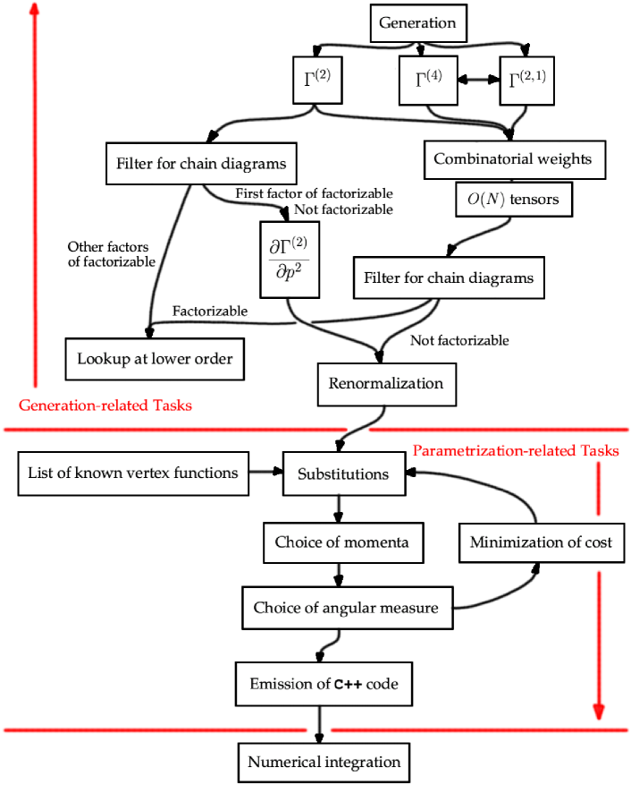
Figure 1: Flowchart of our automatic framework. Its details are clarified in sections 3-4.

In figure 1 we present a flowchart where all the tasks contributing to the structure of our automatic framework are mentioned. Quite schematically, we can identify three main steps: the generation of all needed diagrams with their associated weights and $O(N)$ tensor structure, the parametrization of amplitudes associated to diagrams and, finally, the numerical integration of generated code.

The problem of generating diagrams and combinatorial factors is computationally hard but standard, and will thus be addressed only briefly at the beginning of section 3; the last part of section 3 is devoted to prepare the theoretical ground for section 4, where we present the algorithmic implementation of an efficient strategy to find for each amplitude integral representations with low associated dimensionality. As anticipated, in this paper we will not deal at all with the challenging problem posed by the numerical integration of obtained parametrizations, leaving this task to future publications.

3.2 Graphs, weights and tensors

3.2.1 Representation of graphs

While many good computer packages for manipulating graphs do exist (see for instance [31]), some of them being specifically tailored to applications in theoretical physics (one such example is [32]), we have anyway decided to re-implement our own graph tool from scratch. The main motivation for such an effort can be found in the fact that, since our entire parametrization chain is formulated in terms of graphs, we needed much more extended capabilities than those usually found in usual Feynman-graph manipulation tools; furthermore, we badly needed efficiency, because some of the stages of parametrization production are computationally very expensive (see section 3.6.1 and the end of section 4.3).

All these considerations brought us to the conclusion that only a new library, written in terms of an efficient low-level programming language and providing a set of graph-theoretical operations specifically tailored to our needs, could solve our problems — in the end, C++ has been our final choice of language.

Here are the basic design choices which have been formulated for our library:

• it allows graphs with coloured vertices and coloured lines to be described (in our situation, coloured vertices are used to model external lines and effective vertices —see section 4.2—, while coloured lines are needed i.e. for symmetries of arguments of effective vertices and cosine diagrams, see section 4.4)

• it is based on an adjacency-matrix representation (we briefly recall that for diagrams where only a single kind of lines is allowed, each entry of the adjacency matrix ${\mathcal{A}}_{v,v^{\prime}}$ gives the number of lines joining vertex $v$ and vertex $v^{\prime}$; in more complicated situations ${\mathcal{A}}_{v,v^{\prime}}$ encodes both the number and the colours of such lines)

• it knows the concept of canonical representative for a graph. The basic idea here is the fact that the same graph can have in general different representations, the one obtained from the other by a relabeling of graph vertices; since such a relabeling defines an equivalence relation, the canonical representative is —as usual in similar situations— the special representative picked up to label all the equivalent elements belonging to the same class. It should be noticed that implementing the concept of canonical representative was particularly important in our context: in fact, the definition of the representative can be used to provide an ordering relation for graphs, which is in turn essential to a good cooperation of our library with the data-types and the facilities offered by C++ standard library [33].

  However, while the knowledge of the canonical representative for a graph gives many advantages, it has the main drawback that its computation can turn out to be very expensive (in fact, this operation can imply the inspection of a number of graphs up to the factorial of the number of vertices, such being the maximal number of possible vertex relabelings).

  On the other hand, many algorithms exist which allow to reduce the cost of finding the canonical representative (even if each algorithm known so far suffers from some “difficult” graphs); these algorithms usually consist in “colouring” vertices on the basis of some vertex property which is invariant by vertex relabeling, so to partition the vertex set into smaller subsets, and to reduce —sometimes drastically— the number of permutations to be checked. Our personal choice among the many algorithms proposed in the literature (see for example [34], [35] and [36] for an overview) has been to implement a twofold colouring, based both on leg partitions and on minimal distances (refer to [34] for a description of the latter); these criteria, though being not as efficient for large graphs as those used in [35], are far less complicated from the point of view of software implementation, and nonetheless quite efficient for the small Feynman diagrams we need to cope with.

Some of the graph-theoretical operations provided by our library are for example the identification of connected components, the computation of the order of automorphism group, the computation of spanning trees, the enumeration of all occurrences of a given subgraph in a larger graph (presented as an ordered sequence, that is as an iterator in C++ terminology, see [33]), and the enumeration of all cycles, of all cycle bases and of all paths joining two vertices (in the form of iterators as well). All these capabilities will be essential to implement algorithms presented in section 4.

3.2.2 Generation of graphs

The task of generating all inequivalent graphs which satisfy a predefined set of topological conditions is known since a long time to be a very hard one, due to the fact that all known generation algorithms are also plagued by the problem of isomorphic copies: diagrams corresponding to the same canonical representative are in general produced more than once, leading to a worser and worser inefficiency of the process as the number of vertices of the graph increases. Various methods have been proposed in the literature; here again, some packages are available (see for example [37]). In the spirit of [38], we generate the set of diagrams in a non-recursive way, taking advantage of our knowledge of the canonical representative to prune a large number of isomorphic copies out of the generated tree (see [39]). The performance of such algorithm is very satisfactory, at least for the typical number of vertices we are interested in.

Table 1: Number of diagrams (OPI and without tadpoles) contributing to the two-point and four-point function up to $8$ loops in perturbative order.

• 	Incremental number									Total number
  Loop number	0	1	2	3	4	5	6	7	8	6	7	8
  $\Gamma^{(2,0)}_{\scriptscriptstyle{\mathrm{I}}}$	0	0	1	2	6	19	75	317	1622	103	420	2042
  $\Gamma^{(4,0)}_{\scriptscriptstyle{\mathrm{I}}}$	1	1	2	8	27	129	660	3986	26540	828	4814	31354

In table 1 we quote some results about the number of diagrams needed to compute the two-point and four-point functions. The main facts we can deduce from these numbers are the following:

1. to complete the evaluation of the RG $\beta$-function at $7$-loop level $3986$ more diagrams must be evaluated just for the four-point function $\Gamma^{(4)}_{\scriptscriptstyle{\mathrm{I}}}$ alone

2. improving the computation of anomalous dimensions $\eta_{{\scriptscriptstyle{\mathrm{M}}}}$ and $\eta_{2{\scriptscriptstyle{\mathrm{M}}}}$ in terms of $g_{{\scriptscriptstyle{\mathrm{I}}}}$ to $8$ loops would require the evaluation in $\boldsymbol{p}=\boldsymbol{0}$ of both values and derivatives w.r.t. $p^{2}$ of the $1622$ diagrams contributing to $\Gamma^{(2,0)}_{\scriptscriptstyle{\mathrm{I}}}$, plus —eventually— the evaluation of diagrams contributing to $\Gamma^{(2,1)}_{\scriptscriptstyle{\mathrm{I}}}(\boldsymbol{p}=\boldsymbol{q}=\boldsymbol{0})$. (For a more precise statement of the problem, please refer to the discussion at the end of section 2.2.) These diagrams have more lines and, accordingly, are more difficult to evaluate than those contributing to the seven-loop four-point function, see section 5.

In any case, results in table 1 state clearly that neither of the two tasks presented above can be performed without the help of an automated framework, able to supply the parametrization and the evaluation of all needed amplitudes.

3.2.3 Symmetry factors

When generating Feynman diagrams for the perturbative expansions of correlators in quantum field theories, one is interested in describing graphs whith unlabeled internal vertices, and unlabeled lines as well, because graphs differing by such relabelings contribute with the same amplitude; this causes the problem of computing the symmetry factor for a given Feynman graph, which accounts for the multiplicity of such identical contributions.

Practical computation of symmetry factors can be very difficult, since it requires the knowledge of the order of the automorphism group of the graph of interest; in our case, symmetry factors are derived directly from the adjacency-matrix of the graph, following the directions given in [40].

3.2.4 $O\left(N\right)$-factors

The computation of traces for $O(N)$ group is quite simple, and can be carried out in many ways; for example, tensors can be represented as graphs, and their contractions can be performed in full graphical form as well. Since this point does not pose particular problems, we will not insist on it here.

3.2.5 Consistency checks

Of course, all possible precautions must be taken against the unpleasant possibility of accidentally omitting a graph, or computing a wrong symmetry/$O(N)$ factor. The consistency of our results has been carefully checked in many ways; among them we recall the fact that from zero-dimensional field theory some sum rules can be deduced, allowing to test both combinatorial and $O(N)$ factors (see [14] for a description of this technique). As an aside, we notice that the introduction of a mass counterterm in such a context allowed us to directly obtain sum rules for diagrams without tadpoles (and an analogous solution has apparently been adopted in [22]).

3.3 Which parametrization to choose?

Ideally, in our approach to the computation of RG-functions the “optimal” parametrization for a given Feynman amplitude is the one minimizing the CPU-time which is needed for its numerical evaluation, up to the desired precision. In practice, many factors come into play while trying to quantify in a precise way the various contributions to such a computational cost; for example:

• for a given amplitude, any choice of parametrization induces its own integral representation, with its associated specific dimensionality

• an estimate of the number of evaluations of a given integrand needed to compute the value of a multidimensional integral within a specified numerical accuracy is in general not precisely known a priori, since it depends in an unaccessible way on the regularity properties of the integrand function itself

• parametrizations of the same amplitude in terms of integrals of the same dimensionality may be obtained —see section 4.2— by choosing in various ways the set of replaced effective-vertex functions; these functions may have in general very unequal evaluation timings

• the same vertex function may possibly require a very different amount of floating-point operations when it is evaluated at different values of external momenta.

All these considerations suggest that we should not rely on a too much refined definition of the cost function whose minimum characterizes the optimal parametrization; on the other hand, the typical asymptotic behavior of the error estimate in deterministic multidimensional numerical integration,

$$\mathrm{error}\sim(\mathrm{integrand\ evaluations})^{-{\mathrm{constant}}/{\mathrm{dimensionality}}},$$ (33)

suggests that it is the dimensionality of the integration which sets the basic scale of the number of required evaluations of the integrand. Thus, we will discard all other possible definitions, basically sticking as our cost function to the dimensionality of the final integral needed to compute an amplitude — even if for technical reasons the actual definition (given in section 4.1 and used throughout the article) will need to be slightly more refined, its spirit remains the same.

Having in mind from now on the goal of minimizing the dimensionality of the integral representations of our amplitudes, let us evaluate such a dimensionality for four standard families of parametrizations: we will thus compute the basic cost of momentum representation (${\mathcal{BC}_{\mathrm{Momentum}}}$), that of position representation (${\mathcal{BC}_{\mathrm{Position}}}$), and those of Schwinger (${\mathcal{BC}_{\mathrm{Schwinger}}}$) and Feynman (${\mathcal{BC}_{\mathrm{Feynman}}}$) representations. Such costs are here called basic to stress the fact they refer to the dimensionality of integrals as directly obtained from standard parametrization techniques, without considering the possible use of additional special simplifications (in the case of momentum representation, for instance, a more refined choice of angular measure could be supplied; such a choice will indeed play an important role in lowering the number of residual integrations, as described in section 4.4).

Let us consider a connected OPI diagram ${\mathfrak{D}}$ with ${E}$ external lines, ${{V}}$ internal vertices (${{V}}=:{V_{4}}+{V_{2}}$, ${V_{2}}$ and ${V_{4}}$ being the number of vertices with $2$ and $4$ legs, respectively), ${{L}}$ loops and ${{I}}$ internal lines. The corresponding $d$-dimensional Feynman amplitude ${\mathcal{A}_{\mathfrak{D}}}$ evaluated at zero external momenta and unitary masses can be schematically written in terms of momentum, position, Schwinger and Feynman representations as (respectively):

$${\mathcal{A}_{\mathfrak{D}}} \propto\int\prod_{l=1}^{{{L}}}d^{d}\ell_{l}\;\prod_{i=1}^{{{I}}}\frac{1}{1+k^{2}_{i}}$$ (34)

$$\propto\int\prod_{v=1}^{{{V}}}d^{d}x_{v}\;\delta^{d}(x_{{V}})\prod_{v=1}^{{{V}}}\;\prod_{v^{\prime}=v+1}^{{{V}}}\left({\mathrm{Pr}}(x_{v}-x_{v^{\prime}})\right)^{{\mathcal{A}}_{v,{v^{\prime}}}}$$ (35)

$$\propto\int_{0}^{\infty}\prod_{i=1}^{{{I}}}d\alpha_{i}\;\frac{e^{-\sum_{i}\alpha_{i}}}{\left(Q_{{L}}({\underline{\alpha}})\right)^{\frac{d}{2}}}$$ (36)

$$\propto\int_{0}^{1}\prod_{i=1}^{{{I}}}d\alpha_{i}\;\delta(\sum_{i}\alpha_{i}-1)\;\left(Q_{{L}}({\underline{\alpha}})\right)^{-\frac{d}{2}},$$ (37)

where we denoted by $\ell_{l}$ the loop momenta, by $k_{i}$ the momentum flowing in the $i$-th internal line —which can be expressed as an appropriate linear combination of loop momenta—, by ${\mathrm{Pr}}(x)$ the propagator in position space, by ${\mathcal{A}}_{v,{v^{\prime}}}$ the entries of the adjacency matrix —i.e., the number of lines connecting vertex $v$ to vertex $v^{\prime}$—, and by $Q_{{L}}({\underline{\alpha}})$ an appropriate homogeneous function of $(\alpha_{i})_{i=1}^{{{I}}}$ of degree ${{L}}$ (see e.g. [29] for more details).

Before moving to the evaluation of the basic costs for these integral representations, a useful property of $SO(d)$-invariant integrands must be mentioned (see section 4.4.2 for a more detailed illustration in the case $d=3$). When integrating a function over a collection of vectors $v_{1},\,\ldots\,,\,v_{K}\in\mathbb{R}^{d}$, the dimensionality of the original integral can be reduced in a standard way if the integrand function depends only on the scalar products among those vectors; the reduction is obtained by performing the trivial angular integrations which correspond to the invariance w.r.t. a global $SO(d)$ rotation of integration vectors $v_{1},\,\ldots\,,\,v_{K}$. If $\mathrm{K}\geq d-1$, the number of such trivial integration is ${d(d-1)}/{2}$. Due to vanishing external momenta we evaluate amplitudes at, this property can be applied to momentum representation (34) as well as to position representation (35).

With this property in mind, we are now ready to complete the evaluation of basic costs: the dimensionality of the integral required by each representation follows from previous expressions, by properly taking into account the delta functions in (35), (37), and by making use of the $SO(d)$-symmetry of (34), (35) (corresponding estimates (38), (39) hold for ${{L}}\geq d-1$ and ${{V}}\geq d$, respectively):

$${\mathcal{BC}_{\mathrm{Momentum}}} =d{{L}}-\frac{d(d-1)}{2}$$ (38)

$${\mathcal{BC}_{\mathrm{Position}}} =d\left({{V}}-1\right)-\frac{d(d-1)}{2}=d\left({{L}}+\frac{{E}-3-d}{2}+{V_{2}}\right)$$ (39)

$${\mathcal{BC}_{\mathrm{Schwinger}}} ={{I}}=2{{L}}+\frac{{E}-4}{2}+{V_{2}}$$ (40)

$${\mathcal{BC}_{\mathrm{Feynman}}} ={{I}}-1=2{{L}}+\frac{{E}-4}{2}+{V_{2}}-1;$$ (41)

it should be noticed that the standard topological identities

$${V_{4}} ={{L}}+\frac{{E}-2}{2}$$ (42)

$${{I}} =2{{L}}+\frac{{E}-4}{2}+{V_{2}}$$ (43)

have been used to eliminate ${V_{4}}$ and ${{I}}$ from formulas (39–41).

From expressions (38-41) it clearly appears that, when $d>2$ and the number of loops ${{L}}$ is large enough, ${\mathcal{BC}_{\mathrm{Feynman}}}<{\mathcal{BC}_{\mathrm{Momentum}}}\sim{\mathcal{BC}_{\mathrm{Position}}}$.

Table 2: Basic costs $({\mathcal{BC}_{\mathrm{Momentum}}},{\mathcal{BC}_{\mathrm{Position}}},{\mathcal{BC}_{\mathrm{Schwinger}}},{\mathcal{BC}_{\mathrm{Feynman}}})$ —for momentum, position, Schwinger and Feynman representations respectively— of a ${{L}}$-loop amplitude contributing to $\Gamma^{({E},{V_{2}})}$ at $d=3$.

• 	$\Gamma^{(2,0)}$	$\Gamma^{(4,0)}$	$\Gamma^{(2,1)}$
  ${{L}}=6$	$(15,12,11,10)$	$(15,15,12,11)$	$(15,15,12,11)$
  ${{L}}=7$	$(18,15,13,12)$	$(18,18,14,13)$	$(18,18,14,13)$
  ${{L}}=8$	$(21,18,15,14)$	$(21,21,16,15)$	$(21,21,16,15)$

In table 2 we reproduce in detail the costs of integrating the $3$-dimensional amplitudes contributing at loop orders ${{L}}=6,7,8$ to $\Gamma^{(2,0)}$, $\Gamma^{(4,0)}$ and $\Gamma^{(2,1)}$. From this analysis of standard representations, the apparent conclusion would be that —in the case of interest— Feynman representation considerably lowers the number of residual integrations if compared to momentum or position representations.

However, the seminal idea —exposed in [20]— which allowed Baker, Nickel, Green and Meiron to obtain in [1]-[2] quite precise $6$-loop estimates of the RG-functions consisted, in fact, in using a non-standard representation of amplitudes in momentum space. This new representation was obtained from the standard one by replacing in the amplitudes as many one-loop subintegrals as possible — corresponding to one-loop subdiagrams of the main diagram; in fact, since the analytic expression of one-loop correlators for non-exceptional momenta is analytically known from the work of Melrose [41], a reduction of $3$ integrations in the basic cost readily follows from each substitution one can make in the original amplitude.

As a matter of fact, if we analyze in more detail the cost ${\mathcal{BC}_{\mathrm{Impr.Mom.}}}$ of momentum representation when it is improved in the spirit of Nickel et al., we soon come to a surprising conclusion. Let us suppose that we have been able to replace in an amplitude, say, ${L_{\mathrm{repl}}}$ analytically known functions, each corresponding to a one-loop subdiagram. Assuming ${{L}}-{L_{\mathrm{repl}}}\geq 2$, so that we can spare $3$ integrations thanks to the overall $SO(3)$-invariance of the amplitude, we then obtain the relation

$${\mathcal{BC}_{\mathrm{Impr.Mom.}}}=3\left({{L}}-{L_{\mathrm{repl}}}-1\right).$$ (44)

Now, the requirement that the obtained parametrization have no more residual integrals than the standard Feynman parametrization is equivalent to the following condition:

$${\mathcal{BC}_{\mathrm{Impr.Mom.}}}\leq{\mathcal{BC}_{\mathrm{Feynman}}}\Leftrightarrow 3{L_{\mathrm{repl}}}\geq{{L}}-\frac{{E}}{2}-{V_{2}}$$ (45)

(notice that in the present context the lower bound on ${L_{\mathrm{repl}}}$ is maximized by $\Gamma^{(2,0)}$). More explicitly, when ${{L}}=7(8)$ the condition ${\mathcal{BC}_{\mathrm{Impr.Mom.}}}\leq{\mathcal{BC}_{\mathrm{Feynman}}}$ reads ${L_{\mathrm{repl}}}\geq 2(3)$ for $\Gamma^{(2,0)}$ and ${L_{\mathrm{repl}}}\geq 2(2)$ for $\Gamma^{(2,1)}$ and $\Gamma^{(4,0)}$: this means that if we are able to perform enough replacements the improved momentum space representation will beat standard Feynman parametrization. This fact motivates the choice —Nickel’s as well as ours— of this representation for amplitudes.

In addition, surprises are not yet over: it turns out that in this representation —complemented with a convenient choice of renormalization scheme— one can naturally take advantage of a whole set of powerful identities and properties. For example, all the occurrences of the two-loop “sunset” diagram can be replaced by the analytic expression of its renormalized counterpart, with a gain of $6$ integrals; but much more can be done. The next sections are devoted to a systematic presentation of a set of additional simplifications and tricks which are well suited to improve this framework. In particular:

• the idea of replacing in the amplitudes some functions known analytically —which we will usually refer to as to effective vertex functions, or as to effective vertices for short— is very powerful, and can be generalized to effective vertices other than the ones which were presumably used by Nickel and coworkers. A detailed analysis of this method and its variations is carried out in section 3.4.

• other identities valid when computing amplitudes at zero external momenta can be used to achieve further reductions in the final dimensionality of some parametrizations; they are analyzed in section 3.5

• a good choice of angular measures —that is, of the way of writing the parametrization of loop integration variables in spherical coordinates— can lead to the analytic integration of a conspicuous number of angles. However, being not explicitly tied to Nickel’s framework this problem is in a sense a more general one, and requires some additional notation which will be introduced only at the beginning of section 4; thus, we postpone this issue to section 4.4

• closely related to the last point, there is the possibility of factoring and computing analytically some easier one-dimensional integrals of chains of propagators; this subject is postponed as well to section 4.4.

However, it goes without saying that this approach to the parametrization of amplitudes also shows some drawbacks.

First of all, it must be stated that we do not know exactly which set of simplification rules has been used in [1]-[2] to lead to such a spectacular reduction of the complexity of the original problem, nor we do know whether such a set can be formulated in terms of simple algorithmic procedures. In fact, only a hint of the basics of effective-vertex technique is given by Nickel and coworkers in their published literature (see [22] and [20]); we have thus tried, so to say, to “reverse-engineer” Nickel’s results —and preprint [22] in particular— to deduce or re-invent the techniques we present here, selecting in the end the ones which seemed to us to be the most appropriate for automation; however, nothing prevents some (perhaps essential) ingredients of the original approach from being possibly very difficult to automate, and very difficult to state in algorithmic form.

Secondly, a related —and much more fundamental— problem posed by this otherwise appealing framework is the fact that its effectiveness cannot be proven a priori: no theorem exists (at least in our knowledge) stating that at a given loop order, for a given set of available effective vertices, some minimal number of replacements will be uniformly obtained for all graphs needed during the evaluation of some field-theoretical quantity; the risk exists that, due to stronger and stronger topological obstructions present in diagrams at higher orders, the set of effective vertices will prove inadequate to satisfactorily reduce some “difficult” graphs. As a matter of fact, a few such graphs requiring more residual integrations than their relatives do appear for some choices of effective vertices and sets of graphs to be parametrized. In the lack of a proof a priori, the effectiveness of the method can be demonstrated only a posteriori with an explicit inspection carried out diagram by diagram; considering the very large number of amplitudes, the large number of different possible replacements for a given diagram and the tempting possibility of increasing the set of effective vertices, once again we arrive at the conclusion that such a complex optimization problem can be successfully analyzed only by means of an automatic framework, capable to handle the problem of minimizing the number of residual amplitudes fastly and more effectively than any human being. In addition, such an approach is the only one able to provide an evolutive set-up if new tricks are found or new parametrization strategies prove themselves to be necessary (one example of such a case could be an hypothetical $8$-loop computation, where one could wish to implement, for instance, a stage choosing the best parametrization among those given by both momentum and Feynman representations).

Consequently, in section 4 we will show how to build a prototype framework to optimize —according to a reasonable choice of simplification rules— the parametrization of a given amplitude, starting from a given set of user-defined effective vertices. As reported on in section 5 and section 6, the knowledge of a small number of effective vertices already leads to very effective parametrizations for the cases ${{L}}=6$ and ${{L}}=7$.

3.4 More on effective vertices

The idea of Nickel et al. of substituting effective vertices in a given amplitude, thus attempting to decrease the number of residual integrations and find a cheaper parametrization, is very general. The underlying hypotheses are the line-locality of momentum representation (that is, the mapping between lines of the diagram and products of corresponding propagators in the integrands), integration over loop momenta, the triviality of renormalization (absence of overlapping divergences, implying that one may replace a divergent block with its renormalized counterpart) and, of course, the knowledge of zero-cost or —more generally— low-cost expressions for effective vertex functions describing subdiagrams of the original amplitude (by zero-cost expression we mean a subgraph which is known in terms of elementary functions and zero integrations, while with low-cost expression we indicate an equivalent integral representation of a subdiagram involving a smaller number of integrations than the one we started with).

Various classes of low-cost vertex functions are available; they will be examined in the following sections.

3.4.1 One-loop functions

As already mentioned, analytic expressions in terms of elementary functions for one-loop functions in $d=3$ are known: following our definition, we say that all such functions are zero-cost effective vertices.

More in detail, in [41] one-loop correlators with ${E}\geq d+1$ legs ($d$ being the integer spacetime dimension) are reduced to a linear combination of one-loop correlators with ${E}=d$ legs (see also [20]). Unfortunately, due to the presence of inverse powers of kinematical determinants in the coefficients of the reductions, such formulas have a range of validity limited to non-exceptional momenta, i.e. to kinematical configurations such that the involved determinants are nonvanishing. One possible way to patch this potentially catastrophic problem is to reject such exceptional points during numerical integration: this strategy —suggested in [20]— has the drawback of requiring the compatibility of point-rejection with the chosen integration algorithm. As a complementary alternative, we developed in [42] a general theoretical framework to deal with reductions of one-loop correlators in all kinematical situations, and we implemented it in an highly-optimized and robust C++ library.

3.4.2 Functions in terms of spectral densities

All higher-loop amplitudes whose expressions can be simplified to reduce the number of residual integrals constitute potentially useful effective vertices.

A first concrete example of such a situation is obtained when considering ${{L}}$-loop amplitudes ${\mathcal{A}_{\mathfrak{D}}}^{(2,0)}(p^{2})$ contributing to $\Gamma_{\scriptscriptstyle{\mathrm{I}}}^{(2,0)}(\boldsymbol{p},-\boldsymbol{p})$: due to their analyticity in the complex $p^{2}$ plane cut at $p^{2}<-M^{2}_{\mathrm{threshold}}$, these amplitudes possess a dispersive one-dimensional integral representation, which —when renormalization is not required— has the standard unsubtracted form

$${\mathcal{A}_{\mathfrak{D}}}^{(2,0)}(p^{2}):=\int\prod_{l=1}^{{{L}}}d^{3}\!\boldsymbol{\ell}_{l}\;\prod_{i=1}^{{{I}}}\frac{1}{k^{2}_{i}+m_{i}^{2}}=\int_{0}^{\infty}\frac{dM^{2}}{p^{2}+M^{2}}\;{\rho_{\mathfrak{D}}}\!\left(M\right)$$ (46)

where the density ${\rho_{\mathfrak{D}}}$ is related via Cauchy theorem to the discontinuity of the amplitude along the $p^{2}$-cut, and can be obtained in terms of a sum over cuts of the diagram ${\mathfrak{D}}$ by use of standard Cutkosky rules (see [43] for a useful introduction to such techniques).

Table 3: Analytic expressions for some densities at $d=3$, adopting the normalizations of (46). In the table we used the notations $M_{12}:=m_{1}+m_{2}$ and $M_{123}:=m_{1}+m_{2}+m_{3}$; $\theta(x)$ is the usual step function. Please remark that in the case of “sunset” diagram a subtracted version of (46) must be employed, while the density for the “double-triangle” diagram is evaluated at $m_{i}=1$.

• ${\mathfrak{D}}$	${\rho_{\mathfrak{D}}}(M)$
  	$\frac{\pi^{2}}{M}\;\theta(M-M_{12})$
  	$2\pi^{4}\left(1-\frac{M_{123}}{M}\right)\;\theta(M-M_{123})$
  	$\frac{2\pi^{4}}{M^{2}\sqrt{M^{2}-3}}\;\log{\left(\frac{\left[6-M^{2}+M\sqrt{M^{2}-3}\right]^{2}}{9(M^{2}-4)}\right)}\;\theta(M-2)$ $+\frac{4\pi^{4}}{M^{2}\sqrt{M^{2}-3}}\;\log{\left(\frac{\left[M-3+\sqrt{M^{2}-3}\right]^{2}}{6(M-2)}\right)}\;\theta(M-3)$

In table 3 we list some examples of $3$-dimensional densities whose expressions can be obtained analytically by integration of cut-diagrams. Notice that due to its UV divergence the sunset diagram must be renormalized, and satisfies in our I-scheme a subtracted version of (46) which can be obtained from it by use of the replacement $1/(p^{2}+M^{2})\rightarrow 1/(p^{2}+M^{2})-1/M^{2}$.

A second possible direction to obtain effective vertices —which exploits the knowledge of densities and the absence of renormalization of the involved amplitudes— is the technique of line-dressing, that we describe schematically below.

Let us suppose that the amplitude ${\mathcal{A}}_{{\mathfrak{D}}^{\prime}}$ corresponding to a connected OPI diagram ${\mathfrak{D}}^{\prime}$ with ${{L}}^{\prime}$ loops is analytically known, with the condition that the mass ${m_{j}^{\prime}}$ associated to the $j$-th propagator is different from all other masses in residual propagators,

$${\mathcal{A}}_{{\mathfrak{D}}^{\prime}}:=\int\prod_{l^{\prime}=1}^{{{L}}^{\prime}}d^{3}\!\boldsymbol{\ell}_{l^{\prime}}^{\prime}\;\left[\mathrm{block}\right]\;\left(\frac{1}{{k_{j}^{\prime}}^{2}+{m_{j}^{\prime}}^{2}}\right);$$ (47)

let us suppose in addition that the amplitude ${\mathcal{A}_{\mathfrak{D}}}^{(2,0)}(p^{2})$ associated to some two-point connected OPI diagram ${\mathfrak{D}}$ admits a spectral representation as the one given in (46). Then the amplitude of the diagram ${\mathfrak{D}}^{\prime\prime}$ obtained by replacing (or, familiarly, “dressing”) the $j$-th line of diagram ${\mathfrak{D}}^{\prime}$ with diagram ${\mathfrak{D}}$,

$${\mathcal{A}}_{{\mathfrak{D}}^{\prime\prime}}:=\int\prod_{l^{\prime}=1}^{{{L}}^{\prime}}d^{3}\!\boldsymbol{\ell}_{l^{\prime}}^{\prime}\;\left[\mathrm{block}\right]\;{\mathcal{A}_{\mathfrak{D}}}^{(2,0)}({k_{j}^{\prime}}^{2}),$$ (48)

can be written as

$${\mathcal{A}}_{{\mathfrak{D}}^{\prime\prime}}=\int_{0}^{\infty}d\!M^{2}{\rho_{\mathfrak{D}}}\!\left(M\right)\;\left({\mathcal{A}}_{{\mathfrak{D}}^{\prime}}|_{m^{\prime}_{j}=M}\right).$$ (49)

The term $\left[\mathrm{block}\right]$ stands for the same ${m_{j}^{\prime}}^{2}$-independent expression in both (47) and (48).

Please bear in mind that we used the —implicit but essential— hypothesis that ${\mathfrak{D}}$, ${\mathfrak{D}}^{\prime}$ and ${\mathfrak{D}}^{\prime\prime}$ need not to be renormalized. Examples of ${\mathcal{A}}_{{\mathfrak{D}}^{\prime}}$ eligible to line-dressing are all the one-loop functions whose expressions are known for non-equal masses (see [41], [20]), in all kinematical configurations (see [42]).

However, it must be noticed that the practical implementation of (49) can be very complicated; thus, we decided for the moment to make use of the technique of line-dressing only in the case of the first two-loop diagram on the left of figure 3, which can be seen as a triangle with one line dressed by a bubble: for this effective vertex, the resulting cost turns out to be $\mathcal{C}=1$.

3.4.3 Low-cost subdiagrams

In some cases, we can take advantage of particular “hidden” symmetries of the diagram we are dealing with to obtain low-cost integral representations for some higher-loop functions, with full dependence on external momenta.

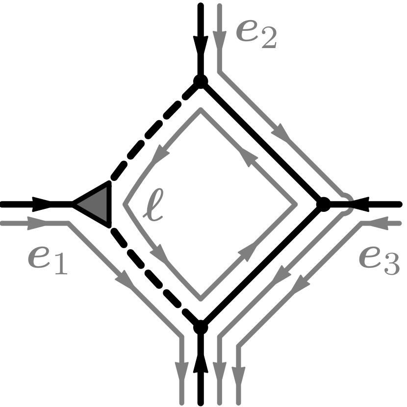
Figure 2: “Square-with-diagonal” diagram, and —on the right— the momentum assignement and the choice of a triangle effective vertex leading to its low-cost parametrization. Please remark that vectors ${\boldsymbol{e}}_{i}$ denote the incoming external momenta.

An example of such a situation is given by the “square-with-diagonal” diagram of figure 2, which —by means of a clever assignement of loop momenta in the spirit of section 4.3— can be parametrized in terms of a one-loop triangular effective vertex and only $2$ residual integrations. In fact, using the momentum assignement described in figure 2 and performing the integral over $\boldsymbol{\ell}$ in spherical coordinates $(|\boldsymbol{\ell}|,\cos\theta,\phi)$ with the $\mathbf{z}$-axis chosen to be parallel to the external momentum $\boldsymbol{e}_{1}$, it turns out that the triangular effective vertex is $\phi$-independent; consequently, the integration over $\phi$ of the two residual propagators factors and can be performed analytically.

The underlying symmetry leading to angular independence is still present in the more general situations of diagrams with two or three external legs, respectively, bordered by an additional chain of propagators connecting two extremal vertices —that is, vertices connected to external lines—; in this sense, in fact, the “square-with-diagonal” diagram can be considered as a triangle bordered by a chain of two propagators. Using in such two general cases a parametrization analogous to that in figure 2, and spherical coordinates oriented as explained above, one readily obtains that the three-leg (resp. two-leg) subblock is $\phi$-independent (resp. $(\theta,\phi)$-independent) and that these angular integrations involve only the propagators belonging to the bordering chain: consequently, such integrations may possibly be done analytically. (As usual, the absence of renormalization is an essential hypothesis for this property to safely hold.) In the case of a two-leg subblock bordered by a chain the considerations above imply that if the angular integral over $(\theta,\phi)$ of the chain of propagators is analytically known one can spare two integrations. The same result can be obtained by the technique of line-dressing one-loop skeletons with the spectral density of the two-leg subblock in question (see section 3.4.2), if this density is available: this latter technique seems more adequate for the implementation of two-loop diagrams corresponding to a one-loop bubble bordered by a chain of propagators.

The parametrization described above turns out to be particularly useful when applied to the family of two-loop diagrams constructed by bordering with a chain two extrema of a triangle one-loop subdiagram; all such diagrams can be evaluated at cost $\mathcal{C}=2$ by performing the integration over $\phi$ of the corresponding chain of propagators, and using the known analytic expression for the triangle subdiagram. The simplest graphs belonging to this family are shown in figure 3 together with some useful bordered bubbles: employed as effective vertices they will prove important, for example, to reduce the complexity of some $7$-loop diagrams back to a more manageable size. Following considerations exposed above, we will assign a cost $\mathcal{C}=1$ only to the first graph, which corresponds to a bubble bordered by a two-line chain or, equivalently, to a line-dressing of a triangle with a bubble density —see section 3.4.2—; even if similar considerations could be applied to the second graph, which is as well a bordered bubble, we will content ourselves to treat it here as an effective vertex of cost $\mathcal{C}=2$, since the development of the code corresponding to the $\mathcal{C}=1$ version would require a much larger programming effort.

Figure 3: Principal two-loop low-cost diagrams (no more than two integrations are required for their evaluation, see discussion in section 3.4.3).

3.4.4 Full-cost subdiagrams

Quite surprisingly, implementing effective vertices as standalone basic blocks can lead to important simplifications even if we are not able to compute the effective vertex in a cheap way and spare integrations; the mere fact that more than one basic block can be replaced in one amplitude is sometimes enough to give rise to reductions in its final cost.

• (a)	(b)	(c)	(d)

Figure 4: A difficult graph together with its treatment.

An enlightening example of such a situation is offered by the diagram shown in figure 4.a; due to its complexity it looks formidable, until one realizes that it can be split as in figure 4.b and expressed in terms of two identical blocks, each having the form illustrated in figure 4.c; thus, the block of figure 4.c can be considered as a new kind of effective vertex with $5$ asymmetric legs, which can be identified and replaced into larger diagrams in the usual way (as illustrated in figure 4.d for the case of diagram of figure 4.a itself).

From a more extensive analysis of figure 4.d —using the definition of cost (56) to deal with the nonzero-cost effective vertices, and computing loop costs as described in section 4— we obtain for this diagram a final cost of $6$ ($3$ for the computation of loop integrals, plus $3$ for the computation of the effective vertices, which is in fact the full cost for computing such two-loop diagrams); on the other hand, it should be noticed that due to topological obstructions only two one-loop ordinary “low-cost” functions could be replaced into the diagram of figure 4.a if we did not introduce the “full-cost” effective vertex of figure 4.c, leading to a much larger final cost of $9$.

3.5 Momentum representation: identities for vanishing external momenta

In this section we collect some simplifying diagrammatic identities, which take advantage of the fact that our amplitudes are always computed at zero external momenta (and that renormalization is trivial in our scheme).

3.5.1 Factorizable amplitudes

Quite often connected OPI diagrams in $\left(\phi^{2}\right)^{2}$ theory show cut-vertices, i.e. —in this context— vertices such that the separation of their four legs into two appropriate groups of two legs disconnects the diagram in two parts.

• $=$

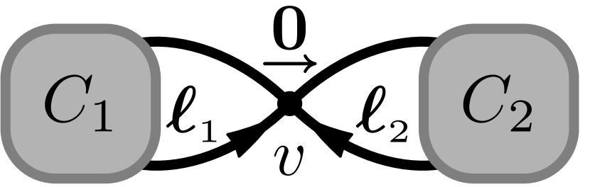
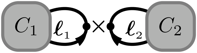
Figure 5: Factorization property of amplitudes of diagrams with cut-vertices when external momenta vanish. The vector $\mathbf{0}$ refers to the vanishing of the momentum flow between the two blocks $C_{1},C_{2}$.

In figure 5 we depicted a cut-vertex $v$, which divides its graph in two subgraphs $C_{1}$ and $C_{2}$. At vanishing external momenta, momentum conservation can be obeyed if and only if there is no total momentum flow from $C_{1}$ to $C_{2}$; using the locality property of momentum representation and an appropriate choice of loop momenta we can always separate the integrations relative to block $C_{1}$ from those relative to block $C_{2}$, expressing the original integral as the product of two integrals, each one associated to a lower order connected OPI diagram evaluated at zero external momenta and carrying a $\int\phi^{2}$ insertion in place of the original $\left(\phi^{2}\right)^{2}$ vertex $v$. In the following we will refer to diagrams with one or more cut-vertices as to factorizable diagrams.

It turns out that a relevant fraction of the diagrams needed to compute RG-functions —about the $20\%$ up to the $7$-loop level— is factorizable in terms of lower-order diagrams; these diagrams are in turn either easier to evaluate than the original one, or already known. This idea is fully implemented in our framework (the corresponding logical block has been labeled as “filter for chain diagrams” in figure 1).

3.5.2 “Quail’s leap”

Other interesting relations can be obtained at zero external momenta when additional symmetries are present in the expression of the amplitude for a given diagram. In fact, it is sometimes possible to look at the diagram in terms of a composition of blocks of propagators, with a momentum flow such that blocks can be rearranged; one can in this way obtain other diagrams, which differ in structure from the starting one but whose associated integrals have the same numerical value at zero external momenta.

• ${\mathcal{A}_{\mathfrak{D}}}=$

  $=$

  $={\mathcal{A}}_{{\mathfrak{D}}^{\prime}}$

Figure 6: An example of “quail’s leap” identity. The dashed lines express here momentum flow between blocks, and do not correspond to real propagators.

In figure 6 we give a pictorial illustration of an example of such set of identities; from now on, we will familiarly call it the “quail’s leap”. The analytic counterpart of figure 6 follows straightforwardly if one writes down the explicit form of amplitudes ${\mathcal{A}_{\mathfrak{D}}}$ and ${\mathcal{A}}_{{\mathfrak{D}}^{\prime}}$ as schematically defined by figure 6, and then relates them using the commutativity of the ordinary product in momentum space; as stated, this leads to the identity

$${\mathcal{A}_{\mathfrak{D}}}=\int d\boldsymbol{\ell}\;A(\boldsymbol{\ell})\,B(\boldsymbol{\ell})\,C(\boldsymbol{\ell})\,D(\boldsymbol{\ell})=\int d\boldsymbol{\ell}\;A(\boldsymbol{\ell})\,C(\boldsymbol{\ell})\,B(\boldsymbol{\ell})\,D(\boldsymbol{\ell})={\mathcal{A}}_{{\mathfrak{D}}^{\prime}}\;.$$ (50)

(It should be noticed here the essential role played by the vanishing of external momenta; this condition automatically enforces momentum conservation in the diagram ${{\mathfrak{D}}^{\prime}}$ associated to the amplitude with permuted blocks.) In spite of the simplicity of its analytic derivation, consequences of “quail’s leap” are non-trivial at all. Starting from the identifications

$\begin{array}[]{c}\includegraphics[width=30.35657pt]{quailA.eps}\end{array}=\begin{array}[]{c}\includegraphics[width=30.35657pt]{quailSDoubleBubble.eps}\end{array}$	$\begin{array}[]{c}\includegraphics[width=30.35657pt]{quailB.eps}\end{array}=\begin{array}[]{c}\includegraphics[width=30.35657pt]{quailSPropagator.eps}\end{array}$
$\begin{array}[]{c}\includegraphics[width=30.35657pt]{quailC.eps}\end{array}=\begin{array}[]{c}\includegraphics[width=30.35657pt]{quailSBubble.eps}\end{array}$	$\begin{array}[]{c}\includegraphics[width=30.35657pt]{quailD.eps}\end{array}=\begin{array}[]{c}\includegraphics[width=30.35657pt]{quailSPropagator.eps}\end{array}$

we can easily show an example of use of the relation in figure 6: substituting the indicated blocks into it we readily get to the following non-trivial diagrammatic identity

$$\begin{array}[]{c}\includegraphics[width=52.03227pt]{quailSOne.eps}\end{array}=\begin{array}[]{c}\includegraphics[width=52.03227pt]{quail-one.eps}\end{array}=\begin{array}[]{c}\includegraphics[width=52.03227pt]{quail-two.eps}\end{array}=\begin{array}[]{c}{\includegraphics[width=52.03227pt]{quailSTwo.eps}}\end{array}.$$

Strictly speaking, it is not guaranteed that the diagrams obtained applying identities such as the one illustrated in figure 6 will belong to the same correlation function as the diagram one starts with; in practice, it turns out that the number of such useful cases does not represent a large fraction of the diagrams required, and this trick is not implemented in the current form of our framework.

3.6 Other aspects of momentum representation

In this section we collect a couple of additional techniques, which, although not leading to a direct reduction in the dimensionality of the integrals to be performed, are nonetheless essential to complete our task of parametrizing amplitudes. In both cases, anyway, we take advantage of momentum representation of amplitudes to put the required manipulations in a neat diagrammatic form. As usual, triviality of renormalization in the I-scheme is tacitly exploited.

3.6.1 The derivative with respect to $p^{2}$

In this section we show how to compute $\left.{\partial\Gamma^{(2,0)}_{\scriptscriptstyle{\mathrm{I}}}}/{\partial p^{2}}\right|_{p=0}$ from the diagrammatic expansion of ${\Gamma^{(2,0)}_{\scriptscriptstyle{\mathrm{I}}}}$ — for a better insight, we keep a generic dimension $d$ in the algebraic expressions presented below.

The derivative w.r.t. $p^{2}$ of a function $f(p^{2})$ can be expressed in terms of derivatives w.r.t. momentum components $p_{\mu}$ by using the chain rule. In particular, the following relation

$$\frac{\partial}{\partial p_{\mu}}\frac{\partial}{\partial p_{\mu}}f\left(p^{2}\right)=2d\frac{\partial}{\partial p^{2}}f\left(p^{2}\right)+4p^{2}\frac{\partial^{2}}{\partial p^{2}\partial p^{2}}f\left(p^{2}\right)$$

turns out to be useful. Assuming in addition $f(p^{2})$ to be smooth at $p^{2}=0$, it follows:

$$\left(\frac{\partial}{\partial p^{2}}f(p^{2})\right)_{p=0}=\frac{1}{2d}\left(\frac{\partial}{\partial p_{\mu}}\frac{\partial}{\partial p_{\mu}}f(p^{2})\right)_{p=0}.$$ (52)

The derivative w.r.t. $p^{2}$ of ${\Gamma^{(2,0)}_{\scriptscriptstyle{\mathrm{I}}}}$ at $p=0$ is obtained by distributing the linear differential operator ${\partial}/{\partial p^{2}}$ over each Feynman amplitude contributing to ${\Gamma^{(2,0)}_{\scriptscriptstyle{\mathrm{I}}}}$ at nonzero $p$, and then applying the identity (52) to each amplitude. (It should be noticed that each amplitude is a function of $p^{2}$ only, and is regular at $p=0$ because all masses in propagators are nonvanishing.) Commuting the derivatives with loop integrals leads us to the problem of evaluating the action of differential operator $\left.{\partial}/{\partial p_{\mu}}\cdot{\partial}/{\partial p_{\mu}}\right|_{p=0}$ on a product of $p$-dependent propagators (obviously, $p$-independent propagators do not take part in the process, and stay unchanged). In the following we will stick to the practically convenient case when the external momentum $p$ flows without fractioning from one external point of the diagram to the other through a chain of propagators (the extension of given formulas to the general case is straightforward).

We label with the index $a$ the lines belonging to the chain, and with the index $b$ the lines not belonging to it; calling $k_{a}$ and $k_{b}$ the internal momenta associated to each line, and using for shortness the notations ${\mathrm{Pr}}(k):=1/(1+k^{2})$, ${\mathrm{Pr}}_{\mu}(k):=k_{\mu}/(1+k^{2})^{2}$, we easily obtain:

$$\left[\frac{1}{2d}\frac{\partial}{\partial p_{\mu}}\frac{\partial}{\partial p_{\mu}}\left(\prod_{a}{\mathrm{Pr}}(p+k_{a})\prod_{b}{\mathrm{Pr}}(k_{b})\right)\right]_{p=0}$$

$$\hbox to0.0pt{\hss${}={}$}\left(\prod_{b}{\mathrm{Pr}}(k_{b})\right)\sum_{a}\left[\left(\frac{4-d}{d}\;{\mathrm{Pr}}(k_{a})^{2}-\frac{4}{d}\;{\mathrm{Pr}}(k_{a})^{3}\right)\;\left(\prod_{a^{\prime}\neq a}{\mathrm{Pr}}(k_{a^{\prime}})\right)\right]$$

$$+\left(\prod_{b}{\mathrm{Pr}}(k_{b})\right)\sum_{a^{\prime}>a}\left[\left(\frac{4}{d}\;{\mathrm{Pr}}_{\mu}(k_{a}){\mathrm{Pr}}_{\mu}(k_{a^{\prime}})\right)\;\left(\prod_{a^{\prime\prime}\neq a,a^{\prime}}{\mathrm{Pr}}(k_{a^{\prime\prime}})\right)\right].$$ (53)

Remarkably, due to the freedom we have in choosing how to parametrize amplitudes the final integrated result will not depend on the choice of the chain; however, it is evident from (53) that to compute the derivative of an amplitude using a chain of length $l$ one must deal with ${l\left(l-1\right)}/{2}+2l$ generalized diagrams — involving, to worsen things, additional two-leg vertices or vector propagators. As a consequence, to get an efficient automated framework for parametrizing amplitudes one must add a stage where all diagrams of ${\Gamma^{(2,0)}_{\scriptscriptstyle{\mathrm{I}}}}$ having a nontrivial dependence on external momentum are scanned; since each chain allows the computation of the derivative w.r.t. $p^{2}$ of the original diagram via the values of the set of graphs induced by (53), the goal will be to find the chain which is “minimal” in terms of the set of integration costs of such induced set of graphs.

This processing stage has been indeed implemented in our code, and is in fact responsible for the majority of the time spent to parametrize the $2$-point function: the large number of chains to be examined, together with the large number of diagrams to be parametrized for each chain, give in general rise to an unpleasant explosion of the number of diagrams to be examined.

We notice as a final remark that a special prescription can be formulated to compute the derivative of factorizable amplitudes which we examined in section 3.5.1: in fact, in this case we can arbitrarily decide to confine the chain of propagators intervening in (53) to the first block of the diagram, that is, to the factored block to which the two external legs of the diagram are connected; in this case, we will obtain the derivative of the whole diagram by computing the derivative (hopefully simpler) of the first block, and then multiplying each of the terms obtained from the r.h.s. of (53) by all the remaining original factored blocks— which will be left untouched by the action of the differential operator ${\partial}/{\partial p^{2}}$, since due to our particular choice of the chain they do not contain any of the propagators involved in the derivation. This consideration explains the intricated structure of the upper part of figure 1.

3.6.2 Insertions of $\int\phi^{2}_{\scriptscriptstyle{\mathrm{I}}}$

The diagrammatic expansion for $\Gamma^{(2,1)}_{\scriptscriptstyle{\mathrm{I}}}({\underline{\boldsymbol{p}}}=\boldsymbol{0};\boldsymbol{q}=\boldsymbol{0})$ can be obtained from that of $\Gamma^{(2,0)}_{\scriptscriptstyle{\mathrm{I}}}({\underline{\boldsymbol{p}}}=\boldsymbol{0})$ by inserting $\int\frac{\phi^{2}_{\scriptscriptstyle{\mathrm{I}}}}{2}$ into each graph which belongs to the $2$-point function; from a diagrammatic point of view this operation corresponds to the insertion of a two-legs vertex (with no additional external momentum), and can be performed by replacing in all possible ways one propagator of the original diagram (that is, one line) with a chain of two propagators; when the same final graph is generated in many different ways, its multiplicity has to be taken into account (see figure 7 for an example).

• $\begin{array}[]{c}\includegraphics[width=88.45619pt]{dotting-one.eps}\end{array}$

  $\longrightarrow$

  $4\times\begin{array}[]{c}\vspace*{-2mm}\includegraphics[width=75.44812pt]{dotting-two.eps}\end{array}+\begin{array}[]{c}\includegraphics[width=75.44812pt]{dotting-thr.eps}\end{array}$

Figure 7: A an example of diagram contributing to $\Gamma^{(2,0)}_{\scriptscriptstyle{\mathrm{I}}}$, and the corresponding groups of diagrams in $\Gamma^{(2,1)}_{\scriptscriptstyle{\mathrm{I}}}$ generated by the insertion of one $\int\frac{\phi^{2}_{\scriptscriptstyle{\mathrm{I}}}}{2}$ operator.

As observed in [22], it turns out from simple topological considerations that these diagrams correspond to a subset of the diagrams of $\Gamma^{(4,0)}_{\scriptscriptstyle{\mathrm{I}}}({\underline{\boldsymbol{p}}}=\boldsymbol{0})$; this fact implies that we do not need to recompute the numerical values for the integrals associated to diagrams of $\Gamma^{(2,1)}_{\scriptscriptstyle{\mathrm{I}}}({\underline{\boldsymbol{p}}}=\boldsymbol{0};\boldsymbol{q}=\boldsymbol{0})$ at some loop order $L$, since such values can be deduced from a lookup in the list of values already computed during the evaluation of the $4$-point function at $L$ loops— this nice property cannot be extended, however, to corresponding symmetry and $O(N)$ factors.

4 Automatic parametrization of amplitudes

We are now ready to examine in full detail how an automatic framework for finding out minimal-cost parametrizations can be built.

4.1 Overview

Provided that the key concept of the method is the substitution of known effective vertices into the analytic expression of the amplitudes, the problem is how to fully exploit such an idea in a systematic, automated and optimal way.

The starting point will be a choice of a set ${\mathbb{E}}:=\{{\mathcal{E}}_{1},\,\ldots\,,\,{\mathcal{E}}_{{N_{\mathrm{ev}}}}\}$ of effective vertex functions. To each effective vertex ${\mathcal{E}}_{e}$ is associated a positive integer $\mathcal{C}_{e}$ called cost. When ${\mathcal{E}}_{e}$ is computed by use of an appropriate integral representation the cost is defined to be the dimensionality of the integration, see (55); otherwise, if the vertex function is known analytically in terms of elementary functions, the cost $\mathcal{C}_{e}$ is zero.

Formalizing now the ideas of section 3.4, once ${N_{\mathrm{ev}}}$ effective vertices have been replaced into the amplitude ${\mathcal{A}_{\mathfrak{D}}}$ corresponding to a given Feynman diagram ${\mathfrak{D}}$, with ${L_{\mathrm{res}}}$ residual loops remaining, the new expression for that amplitude will be given by

$${\mathcal{A}_{\mathfrak{D}}} \propto\int\prod_{l=1}^{{L_{\mathrm{res}}}}d^{3}\!\boldsymbol{\ell}_{l}\;\left(\prod_{j=1}^{{I_{\mathrm{res}}}}\frac{1}{1+k^{2}_{j}}\right)\left(\prod_{e=1}^{{N_{\mathrm{ev}}}}{\mathcal{E}}_{e}\!\left(\mathbb{SP}_{e}\right)\right)$$ (54)

where the effective vertices with non-zero cost are expressed as:

$${\mathcal{E}}_{e}\!\left(\mathbb{SP}_{e}\right):=\int d^{\mathcal{C}_{e}}\!{\underline{\xi_{e}}}\;\;{{\widetilde{\mathcal{E}}}_{e}}\!\left(\mathbb{SP}_{e},{\underline{\xi_{e}}}\right).$$ (55)

${I_{\mathrm{res}}}$ above is the number of residual propagators and $k_{j}$ the momentum flowing in each of them; the set $\mathbb{SP}_{e}\subseteq\left\{\;\boldsymbol{\ell}_{l_{1}}.\boldsymbol{\ell}_{l_{2}}\;|\;l_{1},l_{2}\in 1\ldots{L_{\mathrm{res}}}\mathrm{\ with\ }l_{1}\leq l_{2}\;\right\}$ encodes the dependence of the effective vertex ${\mathcal{E}}_{e}$ in terms of scalar products among loop momenta and plays a key role in the choice of the most appropriate angular measure, as will be shown in section 4.4.

The inclusion of effective vertices with non-zero cost in the set of possible replacements imposes a refinement of the definition of the cost function itself. The problem in question is how to extend the definition of total cost as dimensionality of the involved integration —which is appropriate when the amplitude is expressed in terms of one single multidimensional integral— to situations in which two or more effective vertices with non-zero cost —and, thus, two or more blocks known only in terms of some integral representation— are present in amplitude parametrization and are themselves integrated as in equation (54); the solution to this problem is somewhat implementation-dependent. In the following we will refer to the concrete situation in which the numerical integration of the parametric integrals defining the blocks with non-zero cost via (55) is performed separately for each block, and also separately from that of loop momenta. In the presence of two or more blocks with non-zero cost it seems quite natural —and convenient— to prefer this type of implementation to that based on the opposite strategy of collecting and numerically evaluating all integrations together in a single multidimensional integral.

Following these lines, we will assign to an amplitude parametrization like the one shown in (54)-(55) the refined total cost

$$\mathcal{C}:=\left(\mathrm{loop\ cost}\right)+\left(\max_{1\leq e\leq{N_{\mathrm{ev}}}}\;\mathcal{C}_{e}\right).$$ (56)

The “loop cost” appearing in this expression is given by the still unknown residual dimensionality of the integration of loop variables $\prod_{l=1}^{{L_{\mathrm{res}}}}d^{3}\!\boldsymbol{\ell}_{l}$. It will be the goal of section 4.4 to compute, and possibly minimize, this number.

Some additional comments about formula (56) are in order. First of all, this refined definition of cost can be easily justified by trusting equation (33) and supposing that the number of operations of a sequence of integrations is dominated by the integration(s) of highest dimensionality. Secondly, a finer structure exists: in essence, when a parametrization has a total cost $\mathcal{C}>0$ we can still say that to evaluate it we roughly need a number of operations proportional to those required by a $\mathcal{C}$-dimensional integral; however,

• if we adopt definition (56) for the total cost, a constant proportionality factor in the number of operations is missed in all cases when a parametrization requires the evaluation of more than one single effective vertex having a cost exactly equal to $\max_{1\leq e\leq{N_{\mathrm{ev}}}}\;\mathcal{C}_{e}$

• even in the simple case when only one effective vertex needs to be integrated, and we are then free to choose whether or not to carry out the integration of the effective vertex along with that of loop variables, from the point of view of numerical integration the task of computing $\int_{\mathcal{L}}\left(\ldots\right)\cdot\int_{\Xi}{{\widetilde{\mathcal{E}}}_{e}}$ is not entirely equivalent to that of computing $\int_{\mathcal{L}\times\Xi}\left(\ldots\right){{\widetilde{\mathcal{E}}}_{e}}$ ($\Xi$ being the integration domain of the effective vertex with non-zero cost, and $\mathcal{L}$ the integration domain of loop variables); this happens first of all because more efficient non-separable integration rules can exist allowing to integrate the domain $\mathcal{L}\times\Xi$ as a whole, and then because a higher intermediate precision is in general needed for the evaluations of $\int_{\mathcal{L}}\left(\ldots\right)$ and $\int_{\Xi}{{\widetilde{\mathcal{E}}}_{e}}$ if we want to obtain a given numerical precision for $\int_{\mathcal{L}\times\Xi}\left(\ldots\right){{\widetilde{\mathcal{E}}}_{e}}$.

Nonetheless, since the task of specifying a precise formula for the computation of the cost is indeed a very difficult one —in the light of considerations carried out in section 3.3— we will stick to simpler formula (56) throughout all this article.

Consequently, having picked up a set of known effective vertices ${\mathbb{E}}$ with associated costs $\{\mathcal{C}_{1},\ldots\,,\mathcal{C}_{N_{\mathrm{ev}}}\}$, our strategy to reduce the total cost $\mathcal{C}$ for a given diagram ${\mathfrak{D}}$ will be as follows.

We start by considering the associated amplitude ${\mathcal{A}_{\mathfrak{D}}}$ parametrized in momentum space,

$${\mathcal{A}_{\mathfrak{D}}}\propto\int\prod_{l=1}^{{{L}}}d^{3}\!\boldsymbol{\ell}_{l}\;\prod_{i=1}^{{{I}}}\frac{1}{1+k^{2}_{i}}.$$

Then, we try to reduce the cost (56) by applying the following guidelines:

1. we look among all possible maximal substitutions in the graph ${\mathfrak{D}}$ of subdiagrams from the given set of effective vertices ${\mathbb{E}}$. Each replacement is encoded via an effective graph ${\mathfrak{D}^{*}}$, which contains as many new vertices as possible describing the replaced effective vertices, and gives a new expression for the amplitude in terms of fewer integrals. An algorithm to scan the space of all possible substitutions is presented in section 4.2

2. we reduce the number of scalar products $\boldsymbol{\ell}_{l_{1}}.\boldsymbol{\ell}_{l_{2}}$ our integrand function depends on by means of a careful choice of loop basis (see section 4.3)

3. we maximize the number of trivial angular integrations by selecting the cheapest angular integration measure which is allowed by our previous choices of substitutions and of loop basis (as explained in section 4.4)

4. while picking up the best angular measure, we maximize at the same time the possibilities of factoring away simpler integrals, like for example

   $$\int_{-1}^{1}d\!\left(\frac{\boldsymbol{\ell}_{l_{1}}.\boldsymbol{\ell}_{l_{2}}}{\ell_{l_{1}}\ell_{l_{2}}}\right)\;\left(\frac{1}{1+(\boldsymbol{\ell}_{l_{1}}+\boldsymbol{\ell}_{l_{2}})^{2}}\right)^{n},\;\;\;\;\;n\in\mathbb{N}^{+}$$

   (see as before section 4.4 for more details).

It should be noticed that different (and perhaps more general) strategies can in principle be devised; of course, the list of tricks to minimize the number of residual integrations we just presented is only a faint approximation of what a well-trained “human neural network” can do by examining all diagrams one after the other, and finding out what is likely to be the real optimal parametrization. However, since teaching mathematical intuition to a computer is clearly impossible, what we are interested in here is the much simpler task of creating a fast and robust algorithm relying on a reasonably small number of simplifications, and working reasonably well for the majority of diagrams. A more in-depth discussion about this philosophy and the optimality of the solutions it gives can be found in section 5.

4.2 Substitution of effective vertices

To fulfill our purpose of obtaining parametrizations of a given diagram which have a minimal cost in the sense of equation (56), we must as a first step find out all possible maximal substitutions of effective vertices for that diagram.

Algorithm 1

(Tree of Substitutions) To find out all possible maximal substitutions for a given Feynman diagram ${\mathfrak{D}}$,

1. read the set ${\mathbb{E}}$ of known effective vertices, graphically expressed as pairs

   $$p_{e}\equiv\left\{\;\mathrm{subgraph\ }{\mathfrak{s}}_{e},\mathrm{effective\ graph\ }{\mathfrak{e}}_{e}\;\mathrm{corresponding\ to\ replacement}\;\right\}$$

2. define

   1. the tree of substitutions: to each node is associated a diagram which is obtained by replacing a collection of subdiagrams of ${\mathfrak{D}}$ —non necessarily maximal— with corresponding elements of $\left\{{\mathfrak{e}}_{e}\right\}$; the node also contains the list ${\mathbb{R}}$ of all remaining possible replacements, each one accompanied by a status flag describing whether the related alternative has already been visited or not

   2. the set ${\mathbb{M}}$ of maximal substitutions found so far

   3. the lookup node ${\mathfrak{N}^{*}}$

3. initialize:

   1. create the root node ${\mathfrak{N}_{0}}$ of the tree of substitutions; associate to it diagram ${\mathfrak{D}}$, and a list ${\mathbb{R}}\!\left({\mathfrak{N}_{0}}\right)$ appropriately computed

   2. ${\mathbb{M}}\longleftarrow\emptyset$, ${\mathfrak{N}^{*}}\longleftarrow{\mathfrak{N}_{0}}$

4. if the next unvisited replacement $R$ in the list of replacements ${\mathbb{R}}\!\left({\mathfrak{N}^{*}}\right)$ exists,

   1. update ${\mathbb{R}}\!\left({\mathfrak{N}^{*}}\right)$

   2. apply $R$ to the diagram associated to lookup node ${\mathfrak{N}^{*}}$, thus obtaining a new diagram ${\mathfrak{D}}^{\prime}$

   3. attach a new node $\mathfrak{N}^{\prime}$ to ${\mathfrak{N}^{*}}$; associate to it diagram ${\mathfrak{D}}^{\prime}$, and a list ${\mathbb{R}}\!\left(\mathfrak{N}^{\prime}\right)$ appropriately computed

   4. update the lookup node: ${\mathfrak{N}^{*}}\longleftarrow\mathfrak{N}^{\prime}$

   5. go to step (4)

   else

   1. put the diagram associated to lookup node ${\mathfrak{N}^{*}}$ in the set ${\mathbb{M}}$ of maximal substitutions

   2. do backtrack up to the nearest node whose list of unvisited replacements is not empty;

      if such a node exists,

      1. set that node as the current lookup node

      2. go to step (4)

      else end.

As an example, we now illustrate how algorithm 1 operates when it is applied to the diagram ${\mathfrak{D}}$ and the set of effective vertices ${\mathbb{E}}$ which are presented in figure 8.

• $${\mathfrak{D}}:=\begin{array}[]{l}\includegraphics[width=65.04034pt]{tree1.eps}\end{array}\qquad{\mathbb{E}}:=\begin{array}[]{|l|l|l|l|l|}\hline\cr{\mathfrak{s}}_{e}&\begin{minipage}[c]{52.03227pt}\vspace*{6.5mm}\includegraphics[width=433.62pt]{tree14.eps}\vspace*{1.5mm}\end{minipage}&\begin{minipage}[c]{52.03227pt} \includegraphics[width=433.62pt]{tree15.eps}\end{minipage}&\begin{minipage}[c]{52.03227pt} \includegraphics[width=433.62pt]{tree16.eps}\end{minipage}&\begin{minipage}[c]{52.03227pt} \includegraphics[width=433.62pt]{tree17.eps}\end{minipage}\\ \hline\cr{\mathfrak{e}}_{e}&\begin{minipage}[c]{52.03227pt}\vspace*{1.5mm}\includegraphics[width=433.62pt]{effectiveBubble.eps}\vspace*{1.5mm}\end{minipage}&\begin{minipage}[c]{52.03227pt} \includegraphics[width=433.62pt]{effectiveTriangle.eps}\end{minipage}&\begin{minipage}[c]{52.03227pt} \includegraphics[width=433.62pt]{effectiveSquare.eps} \end{minipage}&\begin{minipage}[c]{52.03227pt} \includegraphics[width=433.62pt]{effectivePentagon.eps}\end{minipage}\\ \hline\cr\end{array}$$

Figure 8: A test case for algorithm (1): a diagram ${\mathfrak{D}}$ and a set of effective vertices ${\mathbb{E}}$ to be replaced in it.

Figure 9: A partial tree of substitutions for the example of figure 8. The order of traversal of each node is explicitly specified between square parentheses. A cross denotes the fact that the corresponding substitution is not possible. The label “Accept” means that the set of replacements associated to the node is maximal.

Figure 10: The complete tree of substitutions for the example of figure 8. The numbers in frame corners indicate the element of the basis of effective vertices which is being replaced into the diagram in each case.

In figure 9 we can observe how the traversal works: the algorithm always tries to push up the level of the tree, in the hope of finding out one effective vertex more in the same lookup diagram. A view of the entire tree (more sketchy) can be found in figure 10. It turns out that for these choices of ${\mathfrak{D}}$ and ${\mathbb{E}}$ there are exactly four possible different maximal substitutions, three with a residual loop number ${L_{\mathrm{res}}}=2$ and one with ${L_{\mathrm{res}}}=3$.

Some general remarks are in order here:

1. we can easily convince ourselves that due to possible topological obstructions the distance from the root of each terminal leaf of the tree of substitutions is not the same. From a different perspective, we can say that the final maximal substitutions will have in general a different number of residual loops, thus leading to parametrizations with a different number of final integrations. The importance of such a conclusion in the perspective of the calculation of cost $\mathcal{C}$ should not be underestimated

2. by taking a closer look to figure 10, it turns out that the tree built up by this naïve formulation of the algorithm must be pruned in order to be used in effective calculations. In fact, it is clear that the same final parametrization can be in general reached following a lot of different branches of the tree: being subdiagrams with a given form but with a different embedding in the diagram distinguishable from each other, the same final set of $n$ vertex functions can be obtained from exactly $n!$ different tree paths. Adding to this problem the observation that this algorithm too is plagued by the problem of isomorphic copies, one can very well understand how the size of such a naïve tree is soon pushed to astronomical values. Luckily, the use of ordered searches for vertex functions brings the complexity of the algorithm back to a manageable size.

4.3 Choice of loop momenta

After a choice of a maximal substitution of effective vertices in the original diagram ${\mathfrak{D}}$ has been performed, resulting in an effective diagram ${\mathfrak{D}^{*}}$, the second step in the generation of parametrizations is clearly the task of assigning loop momenta to ${\mathfrak{D}^{*}}$. In spite of the fact that the choice of loop momenta is often looked at as a trivial operation, a favourable assignement of loop momenta —if complemented by successive optimization of angular measure and maximization of simple angular integrals over residual propagators, see section 4.4 and section 4.4.3— can in many cases provide further reductions in the number of final residual integrations.

The following facts —which are common lore in graph theory— will be very useful to get to algorithm 2, which allows the sequential generation of all possible loop assignments (further references and definitions adapted to more general contexts can be found for example in [44], [45] and [36]).

Definition 1

Given two subdiagrams ${\mathfrak{s}}_{1}$ and ${\mathfrak{s}}_{2}$ of a diagram ${\mathfrak{D}}$, we define ${\mathfrak{s}}={\mathfrak{s}}_{1}\oplus{\mathfrak{s}}_{2}$ as the subdiagram of ${\mathfrak{D}}$ whose lines are present in ${\mathfrak{s}}_{1}$ or in ${\mathfrak{s}}_{2}$, but not in both (exclusive sum of lines).

Definition 2

A $n$-cycle —or $n$-loop in physicists’ terminology— is the diagram composed by the set of vertices $\left\{v_{1},\;\ldots\,,\;v_{n}\right\}$ and the set of distinct lines $\left\{v_{1}-v_{2},\;\ldots\,,\;v_{n}-v_{1}\right\}$. A tree is a connected diagram with no cycles. A spanning tree for a connected diagram is a tree subdiagram with the same vertices as the original diagram; by topological count, the operation of adding a single line to a spanning tree does always produce a subdiagram with loop number equal to $1$.

Theorem 1

Given a connected diagram ${\mathfrak{D}}$, its loops span a vector space $\mathbb{V}\!_{L}$ in $\mathbb{Z}_{2}$ w.r.t. the operation $\oplus$. The dimension of such a vector space is given by ${{L}}$, the number of loops of the diagram familiar to physicists.

Not all the elements of $\mathbb{V}\!_{L}$ are loops, but all the loops of the diagram are contained in $\mathbb{V}\!_{L}$; thus, this theorem gives us a powerful tool to enumerate them all.

Theorem 2

To get a loop basis ${\mathbb{B}}$ for the vector space $\mathbb{V}\!_{L}$ associated to a connected diagram ${\mathfrak{D}}$,

1. produce a spanning tree ${\mathfrak{T}}$ for the diagram

2. for each remaining line ${\mathfrak{l}}\in{\mathfrak{D}}$ such that ${\mathfrak{l}}\in{\mathfrak{D}}$ but ${\mathfrak{l}}\not\in{\mathfrak{T}}$, consider the subdiagram ${\mathfrak{T}}_{{\mathfrak{l}}}$ obtained by adding the line ${\mathfrak{l}}$ to ${\mathfrak{T}}$, that is ${\mathfrak{T}}_{{\mathfrak{l}}}\equiv{\mathfrak{T}}\cup{\mathfrak{l}}$; produce a cycle ${\mathfrak{c}}_{i}$ by identifying it as a subset of ${\mathfrak{T}}_{{\mathfrak{l}}}$.

The set ${\mathbb{B}}\equiv\left\{{\mathfrak{c}}_{1},\ldots\,,{\mathfrak{c}}_{{{L}}}\right\}$ of cycles generated in this way is the desired basis.

As a consequence, we can now formulate the following

Algorithm 2

(Loop bases). To produce all possible assignments of loop momenta in a given connected diagram ${\mathfrak{D}}$

1. build a spanning tree ${\mathfrak{T}}$ for ${\mathfrak{D}}$

2. deduce a first loop basis ${\mathbb{B}}_{1}$ for the loops in the diagram ${\mathfrak{D}}$ by applying theorem 2 to the couple $\left\{{\mathfrak{D}},{\mathfrak{T}}\right\}$; the property ${{{L}}}=\mathrm{card}\left({\mathbb{B}}_{1}\right)$ will hold

3. deduce the set ${\mathbb{L}}$ of all loops contained in the diagram by calculating all possible linear combinations over $\mathbb{Z}_{2}$ of the elements of ${\mathbb{B}}_{1}$ and by discarding combinations that are not loops

4. for each extraction of ${{{L}}}$ loops ${\mathfrak{c}}_{i_{1}},\ldots\,,{\mathfrak{c}}_{i_{{{L}}}}\in{\mathbb{L}}$

   if loops ${\mathfrak{c}}_{i_{1}},\ldots\,,{\mathfrak{c}}_{i_{{{L}}}}$ are linearly independent

   1. take the set $\left\{{\mathfrak{c}}_{i_{1}},\ldots\,,{\mathfrak{c}}_{i_{{{L}}}}\right\}$ as a new possible choice of loop momenta

   2. for each ${\mathfrak{c}}_{i_{n}}$

      1. assign an arbitrary orientation to it

      2. increment (according to the chosen loop orientation) the momenta associated to the lines of ${\mathfrak{c}}_{i_{n}}$ by a quantity $\alpha_{n}\boldsymbol{\ell}_{n}$ — where the $\alpha_{n}$’s are arbitrary non-null coefficients.

As an example of application of algorithm 2 we illustrate in detail the loop parametrization of the “cat’s eye” diagram; it is drawn in figure 13 together with a choice of a spanning tree, ${\mathfrak{T}}$, and with the loop basis ${\mathbb{B}}_{1}$ obtained by applying theorem 2 to ${\mathfrak{T}}$.

• $${\mathfrak{T}}\left(\begin{array}[]{c}\vspace*{-1.5mm}\includegraphics[width=86.72267pt]{catsEye.eps}\end{array}\right)=\begin{array}[]{c}\vspace*{-1.5mm}\includegraphics[width=86.72267pt]{catsEyeSpanningTree.eps}\end{array}$$

  $${\mathbb{B}}_{1}=\left\{\begin{array}[]{ccccc}\vspace*{-3mm}\includegraphics[width=86.72267pt]{catsEyeLoopOne.eps}&\begin{minipage}{2.84526pt},\vspace*{7mm}\ \end{minipage}&\includegraphics[width=86.72267pt]{catsEyeLoopTwo.eps}&\begin{minipage}{2.84526pt},\vspace*{7mm}\ \end{minipage}&\includegraphics[width=86.72267pt]{catsEyeLoopThree.eps}\end{array}\right\}$$

• $\left\{0,0,0\right\}$	${\mathfrak{c}}_{1}\equiv\left\{0,0,1\right\}$	${\mathfrak{c}}_{2}\equiv\left\{0,1,0\right\}$	${\mathfrak{c}}_{3}\equiv\left\{0,1,1\right\}$
  $<1$ loops
  ${\mathfrak{c}}_{4}\equiv\left\{1,0,0\right\}$	${\mathfrak{c}}_{5}\equiv\left\{1,0,1\right\}$	${\mathfrak{c}}_{6}\equiv\left\{1,1,0\right\}$	$\left\{1,1,1\right\}$
  			$>1$ loops

• 
  

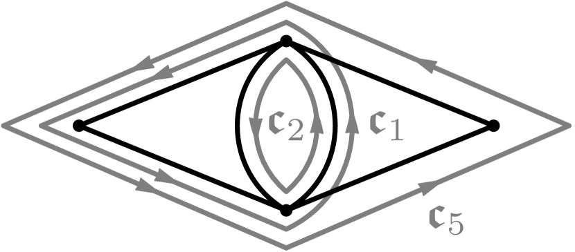
Figure 11: “Cat’s eye” diagram: a spanning tree ${\mathfrak{T}}$ and the associated loop basis ${\mathbb{B}}_{1}$.

Figure 12: “Cat’s eye” diagram: all cycles.

Figure 13: “Cat’s eye” diagram: loop assignment deriving from loop basis ${\mathbb{B}}_{2}\equiv\left\{{\mathfrak{c}}_{1},{\mathfrak{c}}_{2},{\mathfrak{c}}_{5}\right\}$.

The three cycles which are elements of ${\mathbb{B}}_{1}$ are identified (from left to right) with the following basis vectors: $\left\{0,0,1\right\}$, $\left\{0,1,0\right\}$ and $\left\{1,0,0\right\}$. The set of all cycles contained in the original diagram is obtained by working out all possible linear combinations of such basis vectors in $\mathbb{Z}_{2}$, and by discarding the resulting graphs which have more than, or less than, $1$ loop (see figure 13). All possible loop bases will then be given by all choices of three linearly independent loops among the six so far produced: for instance, ${\mathbb{B}}_{2}\equiv\left\{{\mathfrak{c}}_{1},{\mathfrak{c}}_{2},{\mathfrak{c}}_{5}\right\}$ is a valid basis but the same is not true for the choice $\left\{{\mathfrak{c}}_{1},{\mathfrak{c}}_{2},{\mathfrak{c}}_{3}\right\}$, due to the fact that ${\mathfrak{c}}_{3}={\mathfrak{c}}_{1}\oplus{\mathfrak{c}}_{2}$.

Then, given a choice of loop basis and of suitable orientations, momentum assignements for the lines will follow by attributing momenta $\alpha_{1}\boldsymbol{\ell}_{1}$, $\alpha_{2}\boldsymbol{\ell}_{2}$ and $\alpha_{3}\boldsymbol{\ell}_{3}$ (with $\alpha_{i}\neq 0$ arbitrary) to the three cycles of the basis, respectively: in figure 13 we depict the loop choice which is obtained for the “cat’s eye” by choosing the ${\mathbb{B}}_{2}$ defined above.

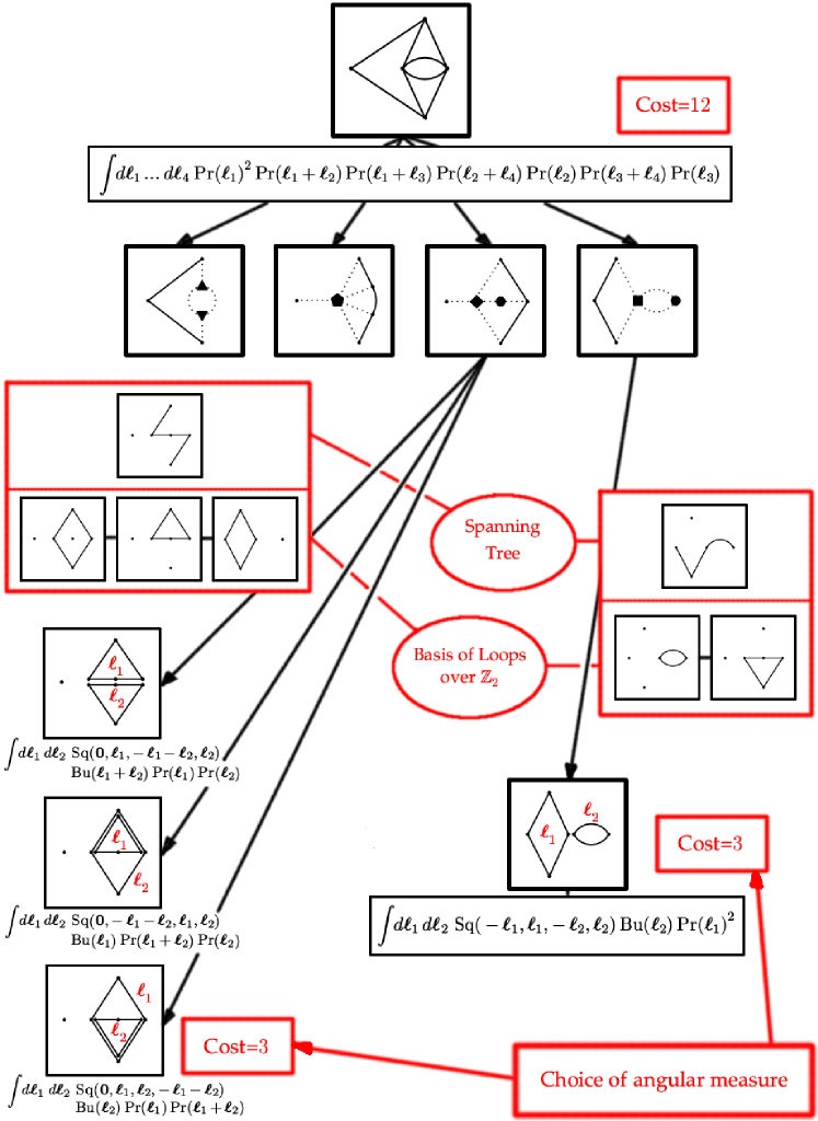
Figure 14: Example of figure 8 after various choices of loop momenta. The costs will be deduced only at a later stage, after angular measures for each diagram have been picked up (see section 4.4).

It should be noticed that even the computation of loop bases can give rise to a combinatorial explosion of generated data, in particular when the number of residual loops ${L_{\mathrm{res}}}$ of the effective diagram ${\mathfrak{D}^{*}}$ is large: this fact can be easily understood by realizing that each loop basis is an extraction of ${L_{\mathrm{res}}}$ linearly independent elements out of a set ${\mathbb{L}}$ composed by up to $2^{L_{\mathrm{res}}}-1$ elements.

Finally, a summary of the entire parametrization procedure for the diagram introduced in figure 8 is presented in figure 14. Please remark that the deduction of the costs shown in this figure relies on the choice of angular measures, which is the subject of the next section 4.4.

4.4 Choice of angular measure

In this section we deal with the problem of explicitly parametrizing the integration measure for an integral expression of the form

$$\mathcal{I}_{F}:=\int\prod_{l=1}^{{L_{\mathrm{res}}}}d^{3}\!\boldsymbol{\ell}_{l}\;F\!\left(\mathbb{SP}\right)$$

where, using notation previously introduced in section 4.1, $F$ depends on a subset $\mathbb{SP}$ of all scalar products $\{\;\boldsymbol{\ell}_{l_{1}}.\boldsymbol{\ell}_{l_{2}}\;|\;l_{1},l_{2}\in 1\ldots{L_{\mathrm{res}}}\mathrm{\ with\ }l_{1}\leq l_{2}\;\}$ among integration vectors.

Since an hyperrectangular domain seems to be the most convenient set-up when we are to perform multidimensional numerical integration, in the following we will restrict ourselves to the particular choice of spherical coordinates, and will accordingly decompose loop vectors as the product of their norm times a versor: $\boldsymbol{\ell}_{l}=\ell_{l}\;\widehat{\boldsymbol{\ell}}_{l}$. Consequently, given an integral

$$\mathcal{I}_{F}=\int\prod_{l=1}^{{L_{\mathrm{res}}}}d\ell_{l}\;\ell_{l}^{2}\;d\Omega_{l}\;F\!\left({\underline{\ell}},\widehat{\mathbb{SP}}\right),$$ (60)

where

$$\widehat{\mathbb{SP}}\subseteq\{\;\widehat{\boldsymbol{\ell}}_{l_{1}}.\widehat{\boldsymbol{\ell}}_{l_{2}}=:\cos\theta_{l_{1}l_{2}}\;|\;l_{1},l_{2}\in 1\ldots{L_{\mathrm{res}}}\mathrm{\ with\ }l_{1}<l_{2}\;\}$$ (61)

$${\underline{\ell}}=(\ell_{1},\,\ldots\,,\,\ell_{L_{\mathrm{res}}}),$$ (62)

we examine here the problem of explicitly writing down an angular measure $\prod_{l}d\Omega_{l}$ which is minimal in the number of required residual integrations, that is, which allows a maximal number of angular integrations to be carried out analytically. Although the spirit of this idea can be easily generalized to a different number of dimensions $d$, our explicit formulas will be specialized to the case $d=3$.

This investigation is motivated by equation (54), which shows that our most general amplitude is precisely of the form just mentioned; the cost (56) associated to a parametrization of a given diagram cannot be fully evaluated without knowing the cost of the integration over loop momenta, and due to this fact one is forced to explicitly determine such a “minimal” angular measure.

It should be noticed that parametrizations of angular measures completely different from the spherical ones can of course be considered —we think e.g. to the techniques used in [46]—, possibly leading as well to a significant reduction in the number of residual integrations; however, we have not considered them in this work, due mainly to the fact that high-performance numerical integrators seem to get along best with simple hyperrectangular domains.

4.4.1 Cosine diagrams

As we will see later on, $\widehat{\mathbb{SP}}$, the subset of scalar products on which function $F$ in equation (60) depends, plays an essential role in determining the optimal choice of angular integration measure. This information is encoded in the so-called cosine diagram associated to function $F$, $\mathfrak{C}$, defined as follows:

1. for each integration variable $\widehat{\boldsymbol{\ell}}_{l}$, add a vertex $v_{l}$

2. if function $F$ carries an explicit dependence on $\widehat{\boldsymbol{\ell}}_{l_{1}}.\widehat{\boldsymbol{\ell}}_{l_{2}}$ (with $l_{1}<l_{2}$), draw a line connecting vertex $v_{l_{1}}$ to vertex $v_{l_{2}}$.

At this level the knowledge of $\widehat{\mathbb{SP}}$ is equivalent to that of $\mathfrak{C}$, but further information —encoding additional properties of $F$— can be attached to the cosine diagram by allowing different kinds of lines in $\mathfrak{C}$. A fruitful application of this technique to the specific class of function we are interested in is postponed to section 4.4.3. In the following section 4.4.2 we will discuss at a more general level the problem of a “good choice” of parametrization of the angular measure.

4.4.2 Choosing axes

The abitual way of parametrizing the angular measure $\prod_{l}d\Omega_{l}$ is to decompose each $d\Omega_{l}$ as

$$d\Omega_{l}=-d\!\left(\cos\theta_{l}\right)d\phi_{l};$$

however, this decomposition requires a previous choice of an axis $\hat{\boldsymbol{z}}_{l}$ —in terms of which angle $\theta_{l}$ is measured— and of an axis $\hat{\boldsymbol{x}}_{l}$ —such that angle $\phi_{l}$ can be defined as in usual $3$-dimensional spherical coordinates. (Please remark that in the following $\hat{\boldsymbol{x}}_{l}$, $\hat{\boldsymbol{z}}_{l}$ will denote a choice of non-degenerate —but not necessarily orthogonal— axis versors.) Once a choice of axes has been picked up, one can explicitly parametrize all the domain of variation of versor $\widehat{\boldsymbol{\ell}}_{l}$ in the standard way as

$$\widehat{\boldsymbol{\ell}}_{l} = \cos\theta_{l}\hat{\boldsymbol{z}}_{l}+\sin\theta_{l}\left(\cos\phi_{l}\;\widehat{\left(\hat{\boldsymbol{z}}_{l}\wedge\hat{\boldsymbol{x}}_{l}\right)\wedge\hat{\boldsymbol{z}}_{l}}+\sin\phi_{l}\;\widehat{\hat{\boldsymbol{z}}_{l}\wedge\hat{\boldsymbol{x}}_{l}}\right)$$

$$\mathrm{with\ }\theta_{l}\in\left[0,\pi\right]\mathrm{\ and\ }\phi_{l}\in\left[0,2\pi\right)$$

(our standard notation $\widehat{\mathbf{v}}:=\mathbf{v}/|\mathbf{v}|$ has been used here). In addition, after a parametrization is given for all versors $\widehat{\boldsymbol{\ell}}_{l}$ one can usefully encode this information in the matrix of scalar products $\left(\mathrm{MSP}\right)$, which is defined as

$$\left(\mathrm{MSP}\right)_{l_{1}l_{2}}\!\!\left({\underline{\theta}},{\underline{\phi}}\right):=\cases{\widehat{\boldsymbol{\ell}}_{l_{1}}.\widehat{\boldsymbol{\ell}}_{l_{2}}\!\!\left({\underline{\theta}},{\underline{\phi}}\right)&if $1\leq l_{1}<l_{2}\leq{L_{\mathrm{res}}}$\\ 0&if $1\leq l_{2}\leq l_{1}\leq{L_{\mathrm{res}}}$.\\ }$$ (64)

(Please remark that ${\underline{\theta}}$ means “an appropriate subset of $\theta_{1},\,\ldots,\,\theta_{L_{\mathrm{res}}}$”, and the same holds for ${\underline{\phi}}$; refer to A for an explanation of our notations.)

Now, supposing we have formulated a choice of axes $\hat{\boldsymbol{x}}_{l},\hat{\boldsymbol{z}}_{l}$ for each $\widehat{\boldsymbol{\ell}}_{l}$ and prepared the matrix of scalar products $\left(\mathrm{MSP}\right)$ associated to this parametrization, the question arises: how many nontrivial angular integrations are necessary to parametrize the angular measure $\prod_{l}d\Omega_{l}$ for a given function $F$ which depends on a (sub-)set of scalar products $\widehat{\mathbb{SP}}$ via a specific cosine diagram $\mathfrak{C}$?

In present framework the answer follows straightforwardly: just use the informations encoded in the cosine diagram $\mathfrak{C}$ and in the matrix $\left(\mathrm{MSP}\right)$ of parametrized scalar products to build up the set $\mathbb{AV}$ containing the “nontrivial” residual angular variables which $F$ really depends on:

$$\mathbb{AV}:=\bigcup_{\mathrm{line}\;l_{1}-l_{2}\;\in\mathfrak{C}}\left\{\;{\underline{\theta}},{\underline{\phi}}\;|\left(\mathrm{MSP}\right)_{l_{1}l_{2}}\mathrm{depends\ on\ variables\ }{\underline{\theta}},{\underline{\phi}}\;\right\}.$$ (65)

The relevance of the set $\mathbb{AV}$ is immediately apparent: given an angular measure $\prod_{l}d\Omega_{l}$ induced by a specific choice for a parametrization, all angular variables ${\underline{\theta}}$, ${\underline{\phi}}$ involved in its realization which are not elements of $\mathbb{AV}$ correspond to flat directions, and can in accordance be trivially integrated out.

Coming back to the issue of parametrization via (4.4.2), it clearly appears that a great arbitrariness is still left over: in fact, given a function $F$ with cosine diagram $\mathfrak{C}$, many choices can be imagined for versors $\hat{\boldsymbol{z}}_{l}$ and $\hat{\boldsymbol{x}}_{l}$, each one leading to an a priori different number of final angular integrations, depending on the particular form of $\mathfrak{C}$.

One result of the present work is the classification of all possible cosine diagrams relevant for integrations up to ${L_{\mathrm{res}}}=4$ and the systematic development of appropriate choices of axes to lower as much as possible the number of final angular integrations. In the following we will clarify the theoretical framework, and introduce the reader to our parametrization strategy by giving some examples.

Let us suppose of having to cope with two integrand functions, $F_{1},F_{2}$ depending respectively on four loop versors $\widehat{\boldsymbol{\ell}}_{1},\,\ldots\,,\,\widehat{\boldsymbol{\ell}}_{4}$ via the set of scalar products $\widehat{\mathbb{SP}}_{1}$ and $\widehat{\mathbb{SP}}_{2}$ defined as:

$$\widehat{\mathbb{SP}}_{1}:=\left\{\;\widehat{\boldsymbol{\ell}}_{1}.\widehat{\boldsymbol{\ell}}_{2},\;\widehat{\boldsymbol{\ell}}_{1}.\widehat{\boldsymbol{\ell}}_{3},\;\widehat{\boldsymbol{\ell}}_{1}.\widehat{\boldsymbol{\ell}}_{4},\;\widehat{\boldsymbol{\ell}}_{2}.\widehat{\boldsymbol{\ell}}_{3},\;\widehat{\boldsymbol{\ell}}_{2}.\widehat{\boldsymbol{\ell}}_{4},\;\widehat{\boldsymbol{\ell}}_{3}.\widehat{\boldsymbol{\ell}}_{4}\;\right\}$$ (66)

$$\widehat{\mathbb{SP}}_{2}:=\left\{\;\widehat{\boldsymbol{\ell}}_{1}.\widehat{\boldsymbol{\ell}}_{2},\;\widehat{\boldsymbol{\ell}}_{1}.\widehat{\boldsymbol{\ell}}_{3}\;\right\}$$ (67)

As a warm-up we consider the natural choice of axes parametrization consisting in picking up two fixed nondegenerate external vectors $\widehat{\boldsymbol{Z}}$ and $\widehat{\boldsymbol{X}}$, and in parametrizing all the versors $\widehat{\boldsymbol{\ell}}_{l}$ w.r.t. these axes via (4.4.2); the following table encodes this possibility.

Axis choices $$\widehat{\boldsymbol{\ell}}_{1} \ldots \widehat{\boldsymbol{\ell}}_{L_{\mathrm{res}}} \hat{\boldsymbol{z}}_{l} \widehat{\boldsymbol{Z}} \ldots \widehat{\boldsymbol{Z}} \hat{\boldsymbol{x}}_{l} \widehat{\boldsymbol{X}} \ldots \widehat{\boldsymbol{X}}$$ (68)

The choice in (68) would lead in the ${L_{\mathrm{res}}}=4$ case to the particular form of $\left(\mathrm{MSP}\right)$ given by

$$\pmatrix{0&\mathrm{c}\theta_{1}\mathrm{c}\theta_{2}+\mathrm{s}\theta_{1}\mathrm{s}\theta_{2}\mathrm{c}\!\left(\phi_{1}-\phi_{2}\right)&\mathrm{c}\theta_{1}\mathrm{c}\theta_{3}+\mathrm{s}\theta_{1}\mathrm{s}\theta_{3}\mathrm{c}\!\left(\phi_{1}-\phi_{3}\right)&\mathrm{c}\theta_{1}\mathrm{c}\theta_{4}+\mathrm{s}\theta_{1}\mathrm{s}\theta_{4}\mathrm{c}\!\left(\phi_{1}-\phi_{4}\right)\cr&0&\mathrm{c}\theta_{2}\mathrm{c}\theta_{3}+\mathrm{s}\theta_{2}\mathrm{s}\theta_{3}\mathrm{c}\!\left(\phi_{2}-\phi_{3}\right)&\mathrm{c}\theta_{2}\mathrm{c}\theta_{4}+\mathrm{s}\theta_{2}\mathrm{s}\theta_{4}\mathrm{c}\!\left(\phi_{2}-\phi_{4}\right)\cr&&0&\mathrm{c}\theta_{3}\mathrm{c}\theta_{4}+\mathrm{s}\theta_{3}\mathrm{s}\theta_{4}\mathrm{c}\!\left(\phi_{3}-\phi_{4}\right)\cr 0&&&0}.$$ (69)

Following equation (65) we readily obtain the sets $\mathbb{AV}_{1,\mathrm{fixed}}$ and $\mathbb{AV}_{2,\mathrm{fixed}}$ of nontrivial angular variables induced by the parametrization (68) for the two cases $F_{1}$, $F_{2}$:

$$\mathbb{AV}_{1,\mathrm{fixed}}=\left\{\;\theta_{1},\theta_{2},\theta_{3},\theta_{4},\phi_{1},\phi_{2},\phi_{3},\phi_{4}\;\right\}$$ (70)

$$\mathbb{AV}_{2,\mathrm{fixed}}=\left\{\;\theta_{1},\theta_{2},\theta_{3},\phi_{1},\phi_{2},\phi_{3}\;\right\}.$$ (71)

According to the above results we are now able to estimate the cost of residual angular integrations as induced by the parametrization (68) to $8$ for $F_{1}$ and to $6$ in the case of $F_{2}$. Impressively enough, the developed formalism reveals quite immediately that due to the simpler angular dependences of $F_{2}$ $2$ angular integrations can be spared w.r.t. the “full cost” case of $F_{1}$. (In fact, a deeper analysis of (69) would show that an additional integration could be spared for both $F_{1}$ and $F_{2}$ since $\left(\mathrm{MSP}\right)$ depends only on differences of $\phi$ variables; however, this point is inessential in the present discussion because —as shown below— one can do much better than that.)

The key that opens the door to much more efficient parametrizations is the possibility to choose as parametrizing axes $\hat{\boldsymbol{z}}_{l}$ and $\hat{\boldsymbol{x}}_{l}$ for $\widehat{\boldsymbol{\ell}}_{l}$ appropriate “moving” reference vectors.

A fruitful example of such a choice is the parametrization defined below, which we call “standard”;

Axis choices $$\widehat{\boldsymbol{\ell}}_{1} \widehat{\boldsymbol{\ell}}_{2} \widehat{\boldsymbol{\ell}}_{3} \ldots \widehat{\boldsymbol{\ell}}_{{L_{\mathrm{res}}}} \hat{\boldsymbol{z}}_{l} {\widehat{\boldsymbol{\ell}}_{1}} {\widehat{\boldsymbol{\ell}}_{1}} {\widehat{\boldsymbol{\ell}}_{1}} {\widehat{\boldsymbol{\ell}}_{1}} \hat{\boldsymbol{x}}_{l} {\widehat{\boldsymbol{\ell}}_{2}} {\widehat{\boldsymbol{\ell}}_{2}} {\widehat{\boldsymbol{\ell}}_{2}}$$ - - - (72)

in the case of ${L_{\mathrm{res}}}=4$ our “standard” choice leads to a cosine matrix $\left(\mathrm{MSP}\right)$ of the form

$$\pmatrix{0&\mathrm{c}\theta_{2}&\mathrm{c}\theta_{3}&\mathrm{c}\theta_{4}\cr&0&\mathrm{c}\theta_{2}\mathrm{c}\theta_{3}+\mathrm{s}\theta_{2}\mathrm{s}\theta_{3}\mathrm{c}\phi_{3}&\mathrm{c}\theta_{2}\mathrm{c}\theta_{4}+\mathrm{s}\theta_{2}\mathrm{s}\theta_{4}\mathrm{c}\phi_{4}\cr&&0&\mathrm{c}\theta_{3}\mathrm{c}\theta_{4}+\mathrm{s}\theta_{3}\mathrm{s}\theta_{4}\mathrm{c}\!\left(\phi_{3}-\phi_{4}\right)\cr 0&&&0}.$$ (73)

Please remark that in the standard parametrization the expression of $\left(\mathrm{MSP}\right)$ in (73) is left unchanged by any legal choice of $\hat{\boldsymbol{x}}_{1}$, $\hat{\boldsymbol{z}}_{1}$ and $\hat{\boldsymbol{x}}_{2}$: that is why no explicit choice is given for such versors in definition (72).

The sets $\mathbb{AV}_{1,\mathrm{standard}}$, $\mathbb{AV}_{2,\mathrm{standard}}$ induced by the standard parametrization (72) for our examples $F_{1}$, $F_{2}$ follow readily:

$$\mathbb{AV}_{1,\mathrm{standard}}=\left\{\;\theta_{2},\theta_{3},\theta_{4},\phi_{3},\phi_{4}\;\right\}$$ (74)

$$\mathbb{AV}_{2,\mathrm{standard}}=\left\{\;\theta_{2},\theta_{3}\;\right\},$$ (75)

resulting in $5$ residual angular integrations for the full-cost case $F_{1}$ and —quite spectacularly— in only $2$ residual angular integrations for the simpler case of $F_{2}$.

From a closer inspection of (72), and of its implications on the matrix of scalar products $\left(\mathrm{MSP}\right)$ —think to (73) and its generalizations— it should appear evident that standard parametrization implements in an explicit way the possibility of making use of the overall $SO\left(3\right)$-symmetry of the integrand to drop the trivial integration over a global $SO\left(3\right)$ rotation of the $\widehat{\boldsymbol{\ell}}_{l}$. In the full-cost case of a function depending on ${L_{\mathrm{res}}}$ vectors $\boldsymbol{\ell}_{l}$ with complete cosine diagram $\mathfrak{C}$, the standard parametrization would give

$$\mathbb{AV}_{\mathrm{standard}}=\left\{\;\theta_{2},\,\ldots\,,\,\theta_{{L_{\mathrm{res}}}},\phi_{3},\,\ldots\,,\,\phi_{{L_{\mathrm{res}}}}\;\right\},$$ (76)

i.e. $2{L_{\mathrm{res}}}-3$ residual angular integrations to which one must add ${L_{\mathrm{res}}}$ integrations over the vector norms, obtaining the total cost $3{L_{\mathrm{res}}}-3$, in agreement with the $d$-dimensional formula introduced in section 3.3. (By the way, a $d$-dimensional generalization of (72) can be straightforwardly derived. See [47] for a similar result from a quite different parametrization.)

The example of function $F_{2}$ above teaches us that when the angular dependence of the function is simple, additional integrations can be spared —within the framework of standard parametrization— compared to the worst-case equation (76); however, to reach this goal, the properly permuted version of the standard parametization (72) must be used, think e.g. to a function $F_{3}$ with $\widehat{\mathbb{SP}}_{3}:=\left\{\;\widehat{\boldsymbol{\ell}}_{1}.\widehat{\boldsymbol{\ell}}_{3},\;\widehat{\boldsymbol{\ell}}_{2}.\widehat{\boldsymbol{\ell}}_{3}\;\right\}$.

All in all standard parametrization (72) proves to be useful to treat a large variety of angular dependencies; however, it should be emphasized that considering other choices of moving axes $\hat{\boldsymbol{x}}_{l}$, $\hat{\boldsymbol{z}}_{l}$ for specific cosine diagrams can sometimes result in parametrizations even cheaper than the standard one.

Let us examine, for instance, the example of an integrand function $F_{4}$ depending on $\widehat{\boldsymbol{\ell}}_{1},\,\ldots\,,\,\widehat{\boldsymbol{\ell}}_{4}$ via a set of scalar products $\widehat{\mathbb{SP}}_{4}:=\left\{\;\widehat{\boldsymbol{\ell}}_{1}.\widehat{\boldsymbol{\ell}}_{2},\;\widehat{\boldsymbol{\ell}}_{1}.\widehat{\boldsymbol{\ell}}_{3},\;\widehat{\boldsymbol{\ell}}_{2}.\widehat{\boldsymbol{\ell}}_{4}\;\right\}$. In this case the standard parametrization (72) would give a set of residual variables

$$\mathbb{AV}_{4,\mathrm{standard}}=\left\{\;\theta_{2},\theta_{3},\theta_{4},\phi_{4}\;\right\},$$ (77)

corresponding to $4$ angular integrations; this result could not be improved by permutations of (72).

On the other hand, the “non-standard” choice

Axis choices $$\widehat{\boldsymbol{\ell}}_{1} \widehat{\boldsymbol{\ell}}_{2} \widehat{\boldsymbol{\ell}}_{3} \widehat{\boldsymbol{\ell}}_{4} \hat{\boldsymbol{z}}_{l} {\widehat{\boldsymbol{\ell}}_{1}} {\widehat{\boldsymbol{\ell}}_{1}} {\widehat{\boldsymbol{\ell}}_{2}} \hat{\boldsymbol{x}}_{l} {\widehat{\boldsymbol{\ell}}_{2}} {\widehat{\boldsymbol{\ell}}_{3}}$$ - - -

leads us to the minimal set of angular variables

$$\mathbb{AV}_{4,\mathrm{non-standard}}=\left\{\;\theta_{12},\;\theta_{13},\;\theta_{24}\;\right\},$$ (78)

corresponding to an angular cost of $3$: two angular integrations are spared w.r.t. the standard parametrization (please remark that in (78) we defined as usual $\theta_{l_{1}l_{2}}:=\arccos\left(\widehat{\boldsymbol{\ell}}_{l_{1}}.\widehat{\boldsymbol{\ell}}_{l_{2}}\right)$).

The variety of parametrizations based on moving axes is enormous, and limited only by the imagination of the user. The only important constraint when giving a choice of axes $\hat{\boldsymbol{x}}_{l}$, $\hat{\boldsymbol{z}}_{l}$ in terms of integration variables $\widehat{\boldsymbol{\ell}}_{l}$ is that —to avoid inconsistences— one must fix an order of integration over the variables $\widehat{\boldsymbol{\ell}}_{l}$ and coherently respect it, by defining $\hat{\boldsymbol{x}}_{l}$, $\hat{\boldsymbol{z}}_{l}$ only in terms of those $\widehat{\boldsymbol{\ell}}_{l^{\prime}}$ which are integrated before $\widehat{\boldsymbol{\ell}}_{l}$ in the chosen integration order.

Given a generic cosine diagram $\mathfrak{C}$, the problem of finding for each $\widehat{\boldsymbol{\ell}}_{l}$ a choice of axes $\hat{\boldsymbol{x}}_{l}$, $\hat{\boldsymbol{z}}_{l}$ giving rise to an angular measure with the minimal number of residual integrations over $\theta$, $\phi$ is —in our knowledge— still unsolved. A partial answer can be found in the following proposition, which deals with cosine diagrams of tree type.

Proposition 1

Given a cosine diagram $\mathfrak{C}$ with ${L_{\mathrm{res}}}$ vertices and vanishing loop number, a choice of axes $\hat{\boldsymbol{x}}_{l}$, $\hat{\boldsymbol{z}}_{l}$ can be given for each $\widehat{\boldsymbol{\ell}}_{l}$ —in the sense of (4.4.2)— such that the angular measure is expressed in terms of ${L_{\mathrm{res}}}$ residual integrations of $\cos\theta$-type (or, equivalently, such that $\mathbb{AV}$ has ${L_{\mathrm{res}}}$ elements, all of $\theta$-type).

Proof Suppose first that $\mathfrak{C}$ is a tree (hence connected by definition). Choose a root vertex $v_{l_{0}}$ on $\mathfrak{C}$. Fix arbitrarily a couple of nondegenerate versors $(\widehat{\boldsymbol{X}},\widehat{\boldsymbol{Z}})$ and assign $(\hat{\boldsymbol{x}}_{l_{0}},\hat{\boldsymbol{z}}_{l_{0}})=(\widehat{\boldsymbol{X}},\widehat{\boldsymbol{Z}})$ for the root vertex and $\hat{\boldsymbol{x}}_{l}=\widehat{\boldsymbol{X}}$ for all other vertices $v_{l}$ of $\mathfrak{C}$. A choice of axis $\hat{\boldsymbol{z}}_{l}$ for all vertices $v_{l}\neq v_{l_{0}}$ will now be given, by iterating over their distance $n$ from the root vertex $v_{l_{0}}$. First define $\hat{\boldsymbol{z}}_{l_{1}}=\widehat{\boldsymbol{\ell}}_{l_{0}}$ for all vertices $v_{l_{1}}$ at distance $1$ from the root — $\widehat{\boldsymbol{\ell}}_{l_{0}}$ being the integration versor associated by definition to the root vertex. Then iterate over increasing $n\geq 1$ as following: for each vertex $v_{l_{n}}$ at distance $n$ define $\hat{\boldsymbol{z}}_{l_{n+1}}=\widehat{\boldsymbol{\ell}}_{l_{n}}$ for all vertices $v_{l_{n+1}}$ departing from $v_{l_{n}}$ and having distance $n+1$ from the root — $\widehat{\boldsymbol{\ell}}_{l_{n}}$ being the integration versor associated by definition to $v_{l_{n}}$. If $\mathfrak{C}$ is not connected repeat the above reasoning for each connected component of $\mathfrak{C}$, using the fact that with this parametrization the angular measure factors in term of angular measures over the connected components of the cosine diagram. $\Box$

In table 4 we will give the complete classification of cosine diagrams for the case ${L_{\mathrm{res}}}=3$, as well as the best choice of parametrizations which we were able to find according to the lines of reasoning presented in this section (including also some additional tricks which will be introduced in the following section 4.4.3).

4.4.3 Cosine diagrams with disconnectible lines

As mentioned in section 4.4.1, it is sometimes useful to encode additional properties of the integrand function $F$ in the cosine diagram $\mathfrak{C}$, by distinguishing different types of lines. This technique comes particularly at hand when parametrizing loop integrations for the amplitudes described in equation (54). Below we identify a particular situation when the integrand function depends on its arguments in a simpler way: an appropriate codification of this information in the cosine diagram and a careful analysis may sometimes lead to the detection of new types of factored analytically-known angular integrals and, consequently, to an additional decrease of the number of residual angular integrations.

The situation of interest is when the integrand function $F$ can be factored as follows:

$$F=\left(\mathrm{block\ with\ no\ dependence\ on\ }\widehat{\boldsymbol{\ell}}_{l_{1}}.\widehat{\boldsymbol{\ell}}_{l_{2}}\right)\left(\frac{1}{1+\ell_{l_{1}}^{2}+\ell_{l_{2}}^{2}+2\;\boldsymbol{\ell}_{l_{1}}.\boldsymbol{\ell}_{l_{2}}}\right)^{n},$$ (79)

$n$ being a strictly positive integer; in this case the line joining vertices $v_{l_{1}}$ and $v_{l_{2}}$ in $\mathfrak{C}$ will be graphically denoted with a dashed style instead of a continuous one, and we will say that such a line —together with the associated cosine $\cos\theta_{l_{1}l_{2}}:={\widehat{\boldsymbol{\ell}}_{l_{1}}.\widehat{\boldsymbol{\ell}}_{l_{2}}}$ between loop momenta $\boldsymbol{\ell}_{l_{1}}$ and $\boldsymbol{\ell}_{l_{2}}$— is disconnectible.

The motivation for introducing the notion of disconnectible lines derives from the following observation: supposing that we have been able to pick up a parametrization of angular measure $\prod_{l}d\!\left(\cos\theta_{l}\right)d\phi_{l}$ such that

1. $\cos\theta_{l_{1}l_{2}}$ belongs to the set of angular integration variables $(\cos\theta_{1},\cdots,\cos\theta_{{L_{\mathrm{res}}}})$

2. the only dependence of the integrand on $\cos\theta_{l_{1}l_{2}}$ is via the scalar product $\widehat{\boldsymbol{\ell}}_{l_{1}}.\widehat{\boldsymbol{\ell}}_{l_{2}}$, i.e. no spurious dependencies on $\cos\theta_{l_{1}l_{2}}$ of other scalar products are re-introduced by the parametrization —see section 4.4.2,

then the integration

$$\int_{-1}^{1}d\!\left(\cos\theta_{l_{1}l_{2}}\right)\;\left(\frac{1}{1+\ell_{l_{1}}^{2}+\ell_{l_{2}}^{2}+2\;\ell_{l_{1}}\ell_{l_{2}}\;\cos\theta_{l_{1}l_{2}}}\right)^{n}$$ (80)

can be factored away and carried out analytically, thus leading to a lower number of required residual integrations.

However, this is not the actual end of the history: a weaker situation can sometimes happen when it is not possible to integrate directly over a disconnectible cosine $\cos\theta_{l_{1}l_{2}}$, but such a cosine can nonetheless be expressed in terms of some of the variables that parametrize the angular measure, with the condition that one of these variables must appear only in the expression of the scalar product $\widehat{\boldsymbol{\ell}}_{l_{1}}.\widehat{\boldsymbol{\ell}}_{l_{2}}$. In this case, again, the integral over such distinguished angular variable of the power of propagators containing $\widehat{\boldsymbol{\ell}}_{l_{1}}.\widehat{\boldsymbol{\ell}}_{l_{2}}$ —see (79)— can be factored and, possibly, performed analitically. A typical example of such a case is given by the combination

$$\int_{0}^{2\pi}d\phi_{3}\;\left(\frac{1}{1+\ell_{2}^{2}+\ell_{3}^{2}+2\;\ell_{2}\ell_{3}\;\widehat{\boldsymbol{\ell}}_{2}.\widehat{\boldsymbol{\ell}}_{3}}\right)^{n}$$

$$\widehat{\boldsymbol{\ell}}_{2}.\widehat{\boldsymbol{\ell}}_{3}=\cos\theta_{2}\cos\theta_{3}+\sin\theta_{2}\sin\theta_{3}\cos\phi_{3},$$ (81)

originating for example in some cases from the “standard” angular parametrization defined in (72); it should be noticed that integrals in the form of (81) can always be performed by means of the technique of complex residues.

Additional complications arise when we want to minimize the number of angular integrations in presence of an integrand function $F$ whose associated cosine diagram $\mathfrak{C}$ possesses disconnectible lines. As a matter of fact, in this case we must face two different requirements at the same time: as in previous section, we must minimize the number of angular integration variables on which $F$ depends; in addition, we must now maximize as well the number of occurrences of integrals in the form of (80) and (81).

Such a problem is quite complicated, and finding a solution implies the enumeration and the inspection of all possible cosine diagrams with disconnectible lines which can arise up to the maximal number of residual loops ${L_{\mathrm{res}}}$ we are interested in.

Table 4: Our choice of “cheapest” angular measures for the case ${L_{\mathrm{res}}}=3$. See the text for all the explanations about graphical conventions used in this table.

• Initial cosine diagram	Final cosine diagram	Variables lines depend on	Cost
  			$(0,0)$
  			$(0,0)$
  		line $1$–$2$ $\longrightarrow$ $\left\{\theta_{2}\right\}$	$(1,0)$
  			$(0,0)$
  		line $1$–$2$ $\longrightarrow$ $\left\{\theta_{2}\right\}$	$(1,0)$
  		line $1$–$2$ $\longrightarrow$ $\left\{\theta_{2}\right\}$ line $1$–$3$ $\longrightarrow$ $\left\{\theta_{3}\right\}$	$(2,0)$
  		line $1$–$2$ $\longrightarrow$ $\left\{\theta_{2}\right\}$ line $1$–$3$ $\longrightarrow$ $\left\{\theta_{3}\right\}$	$(2,0)$
  		line $1$–$2$ $\longrightarrow$ $\left\{\theta_{2}\right\}$ line $1$–$3$ $\longrightarrow$ $\left\{\theta_{3}\right\}$	$(2,0)$
  		line $1$–$2$ $\longrightarrow$ $\left\{\theta_{2}\right\}$ line $1$–$3$ $\longrightarrow$ $\left\{\theta_{3}\right\}$	$(2,0)$
  		line $1$–$2$ $\longrightarrow$ $\left\{\theta_{2}\right\}$ line $1$–$3$ $\longrightarrow$ $\left\{\theta_{3}\right\}$ line $2$–$3$ $\longrightarrow$ $\left\{\theta_{2},\theta_{3},\phi_{3}\right\}$	$(2,1)$

To give a taste of how things look like, we illustrate in table 4 the “simple” case ${L_{\mathrm{res}}}=3$. In the first column, all possible cosine diagrams are listed; a dashed line means that the associated cosine is disconnectible in the sense defined by equation (79). As explained above, in some cases the corresponding angular measures can be simplified by analytically integrating over appropriate angles; thus, in the second column “improved” cosine diagrams can be found, describing the cheapest measures which will be used in the final parametrization; in this column dashes mean “a $\theta$ has been integrated” —see (80)—, while dots mean “a $\phi$ has been integrated” —see (81)—. In the third column one can see the contribution to the set $\mathbb{AV}$ coming from each line of the improved cosine diagram — see (65). Finally, in the last column we indicate the cost of the final angular measure as a couple $($number of integrations on ${\underline{\theta}}$, number of integrations on ${\underline{\phi}}$$)$.

We just mention that in the more realistic case of ${L_{\mathrm{res}}}=4$ we have $65$ different possible cosine diagrams, which have been analyzed by hand and, successively, incorporated in our code. In addition, the program takes automatically care of the fact that at ${L_{\mathrm{res}}}=4$ each basic cosine diagram can manifest in up to $4!=24$ different possible permutations.

5 Implementation, and results

The techniques described in section 4 were actually used to produce a C++ program; given a graphical description of the basis of effective vertices one intends to use —as described in section 4.2—, and a specification of the set of diagrams to be parametrized, our code produces

• an histogram of the distribution of the cost $\mathcal{C}$ —as defined in section 4.1— for the specified set of diagrams whose parametrization has been required. Examples of such distributions for some different choices of diagrams and bases of effective vertices can be found in figure 15, figure 16 and figure 17

• the C++ functions needed to perform the numerical integration of amplitudes, ready to be compiled if an actual numerical implementation of each of the effective vertices which have been used during the parametrization stage is given; the set of amplitudes is then placed in a dynamical library, with each subroutine ready to be retrieved by the integration program. We do not enter here into the very complicated details of numerical evaluation of amplitudes, which will be described in future publications

• the specifications needed to compute the RG functions $\beta_{\scriptscriptstyle{\mathrm{M}}}(g_{\scriptscriptstyle{\mathrm{M}}}),\eta_{\scriptscriptstyle{\mathrm{M}}}(g_{\scriptscriptstyle{\mathrm{M}}}),\eta_{2{\scriptscriptstyle{\mathrm{M}}}}(g_{\scriptscriptstyle{\mathrm{M}}})$; these informations consist in a list of all required combinatorial and $O\left(N\right)$- factors, plus —after a suitable file containing the results of numerical integration has been provided— the actual value of each integral in question, with an estimation of its numerical error.

In general, the program presents a lot of useful switches to precisely tune its behaviour: for example, subsets of all the needed graphs —or even single graphs— can be selected to be parametrized, and a graphical automated output containing all the details of the process is provided for debugging purposes if requested; more than one parametrization for the same amplitude can be produced and stored when a comparison is desired.

The code consists of about $14.000$ lines of C++ —about $7.000$ for graph library and other auxiliary libraries, the rest in higher-level routines for the manipulation of scalar amplitudes— which have been written and tested from scratch. Being modular in the spirit of C++ classes (see [33]) —with a different class corresponding to each different concept exposed in section 4, like substitutions of effective vertices, loop bases, angular measures and so on— the code can be quite easily modified to include new computational simplifications or new strategies, as discussed in section 4.1. On a typical machine of the GHz-era, the $7$ loops can be entirely parametrized —and the corresponding C++ code produced— in some hours; peak memory occupation is entirely acceptable.

Some additional details about the structure, the design and the results of the program which we had to omit here due to the lack of space can be found in [40] (although it documents a slightly outdated version of our framework): for example, the explicit parametrization of all amplitudes up to the $4$-loop level with “simple” one-loop effective vertices can be found there.

• 

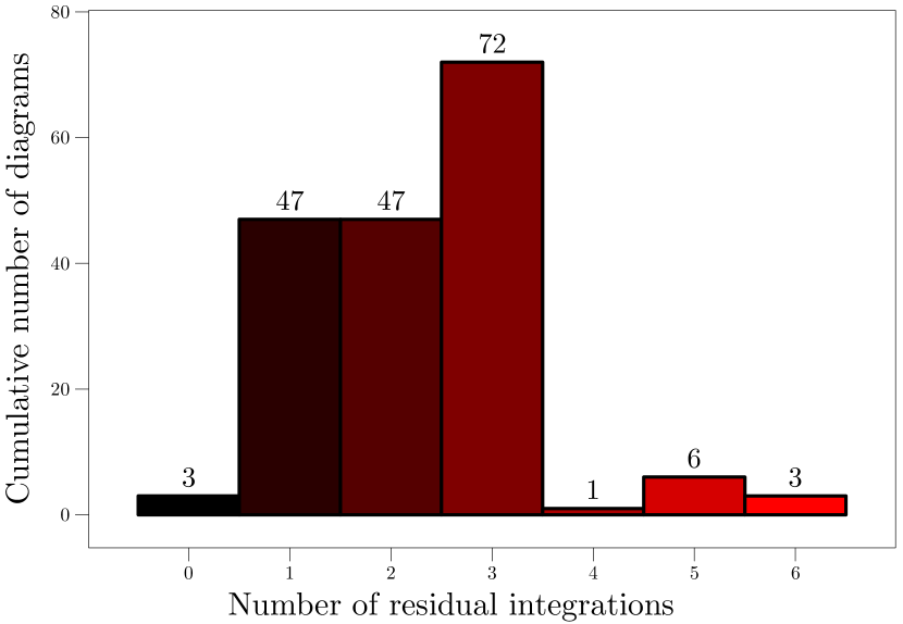
Figure 15: Total cost of loops from $1$ to $5$. The histogram accounts for amplitudes contributing to $\Gamma^{(2,0)}_{\scriptscriptstyle{\mathrm{I}}}$, $\partial\Gamma^{(2,0)}_{\scriptscriptstyle{\mathrm{I}}}/\partial p^{2}$ and $\Gamma^{(4,0)}_{\scriptscriptstyle{\mathrm{I}}}$, including higher-points amplitudes obtained from factorization — see section 3.6.2 and section 3.5.1. Used basis of effective vertices are $1$-loop functions up to the pentagon (see figure 8) plus $2$-loop functions of figure 3, plus the renormalized sunset.

• 

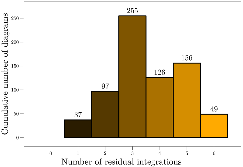
Figure 16: Total cost of the $6$-th loop alone. The histogram accounts for amplitudes contributing to $\Gamma^{(2,0)}_{\scriptscriptstyle{\mathrm{I}}}$, $\partial\Gamma^{(2,0)}_{\scriptscriptstyle{\mathrm{I}}}/\partial p^{2}$ and $\Gamma^{(4,0)}_{\scriptscriptstyle{\mathrm{I}}}$, including higher-points amplitudes obtained from factorization — see section 3.6.2 and section 3.5.1. Used basis of effective vertices are $1$-loop functions up to the pentagon (see figure 8) plus $2$-loop functions of figure 3, plus diagram of figure 4.c, plus the renormalized sunset.

• 
• 

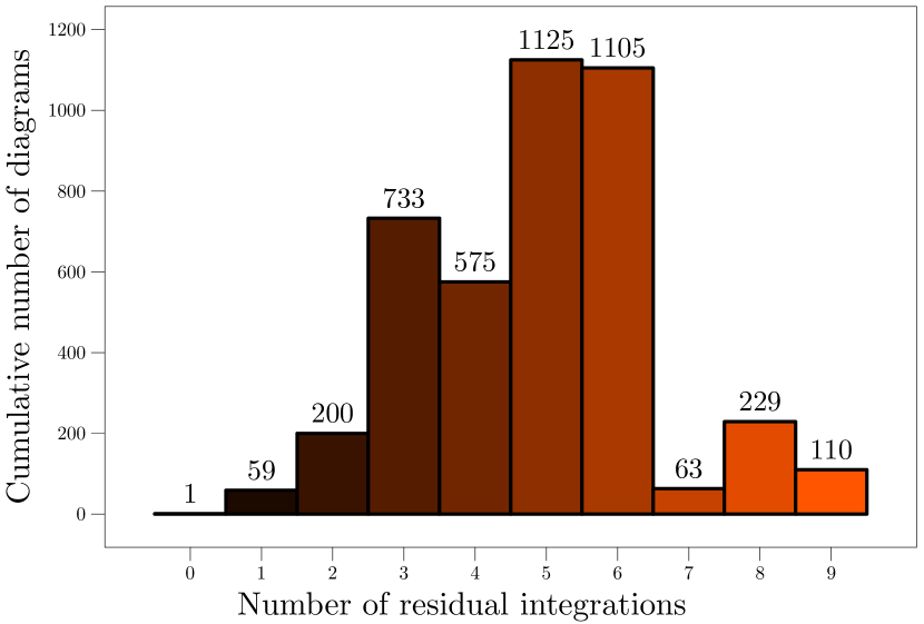
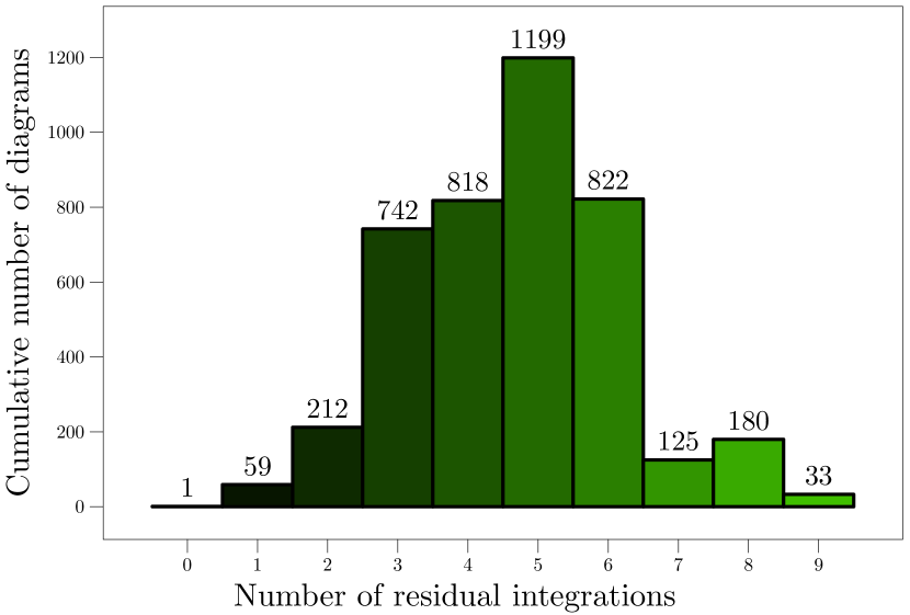
Figure 17: Total cost of the $7$-th loop alone. The histogram accounts for amplitudes contributing to $\Gamma^{(2,0)}_{\scriptscriptstyle{\mathrm{I}}}$, $\partial\Gamma^{(2,0)}_{\scriptscriptstyle{\mathrm{I}}}/\partial p^{2}$ and $\Gamma^{(4,0)}_{\scriptscriptstyle{\mathrm{I}}}$, including higher-points amplitudes obtained from factorization — see section 3.6.2 and section 3.5.1. Used bases of effective vertices are: above, $1$-loop functions up to the pentagon (see figure 8) plus the renormalized sunset; below, $1$-loop functions up to the pentagon, plus $2$-loop functions of figure 3, plus diagram of figure 4.c, plus the renormalized sunset.

We would now like to discuss in detail some of the typical results produced by the program.

Two histograms detailing the costs of the parametrization of amplitudes for loops $1$ to $5$ all together, and for loop $6$ alone, respectively, are shown in figure 15 and figure 16; the basis of functions employed here is a “standard” one, composed by the polygons up to the pentagon, the renormalized “sunset” effective vertex, all other low-cost $2$-loop functions shown in figure 3 (see section 3.4.3) and —from $6$ loops and higher— the effective vertex corresponding to the $2$-loop diagram of figure 4.c. All resulting costs are not more than $6$; this fact is in agreement with what has been previously found by Nickel et al., who declare in [22] that they were able to obtain all their parametrizations of $6$-loop diagrams with integrations in not more than $6$ residual dimensions.

In spite of the fact that we are working in different renormalization schemes and that, consequently, we have a different number of diagrams to evaluate, it would be nevertheless quite interesting to be able to perform a more precise quantitative comparison between our histograms and the corresponding distributions obtained by Nickel and coworkers; however, this information has never been published. Our general impression is that our results could be slightly sub-optimal, mainly due to the fact that for some “difficult” graphs it is probably possible to work out cheaper parametrizations by hand, in the spirit of figure 4. All in all, the results we obtained for the $6$-loop case can be also interpreted as being very encouraging, if one bears in mind that

• the simplifications implemented in our code (see the list in section 4.1) are just a few, and not very complicated; nonetheless, they are enough to obtain a set of parametrizations which would seem comparable to that derived in the original work of Nickel and coworkers

• our program is very general, so that other techniques can be easily added if needed

• a separate treatment of a few particularly expensive graphs is always possible

• if we want to tackle the computation of the $7$-th loop, we must be anyway prepared to the appearance of a consistent number of integrals with a residual dimensionality much larger than $6$.

Going on to the results relative to the parametrization of the $7$-th loop shown in figure 17 —which are the most important since their knowledge represents the motivation for this work, in view of their possible use to improve available estimates of critical quantities— the situation looks even more promising. The larger residual dimensionality is here $9$, still low enough to make possible a high-precision numerical evaluation of the amplitudes if enough computer power is available. By comparing the two profiles shown in the figure one can notice how the two-loop effective functions play an essential role in lowering the overall complexity of the computation of a factor of $\sim 3$ (this rough estimate can immediately be obtained by remembering, as explained in section 3.3, that the main part of computer time will be spent in the evaluation of the integrals of highest dimensionality). Such results bring us to the remarkable conclusion that even at a $7$-loop level the approach of Baker, Nickel, Green and Meiron remains fruitful, leading —within the present framework— to an acceptable set of parametrizations for all the required diagrams, including those contributing to the $4$-point function.

As a final remark, some preliminary looks at the corresponding results for the $2$-point functions at $8$ loops (not reported in this article) seem to indicate that the set of effective vertices which allows a successful parametrization of the $7$ loops would not be adequate to conveniently parametrize the $8$ loops; anyway, due to the number and the complexity of required integrals the possibility of carrying out the computation of the $8$-th loop is purely academic at the moment.

6 Epilogue

In this work we present a solution to the problem of building an automated framework for the parametrization of Feynman amplitudes needed to compute —at the level of $7$ loops and higher— the Renormalization-Group $\beta$-function and the anomalous dimensions $\eta,\eta_{2}$ for the $3$-dimensional $O(N)$ vector model.

The core of the employed computational method —in the spirit of [1]-[2]— consists in replacing effective-vertex functions and applying other analytic simplifications to the original expressions for amplitudes in momentum space.

Some of the key features of our own approach, as compared to that in [1]-[2], are the following:

• a different intermediate renormalization scheme —the I-scheme— has been chosen, which has simpler renormalization properties as well as a Callan-Symanzik equation with exactly-known coefficients, see section 2.2

• a systematic treatement of the parametrization of loop integrations in momentum space (leading in our framework to a “good choice of angular measures”) has been developed in section 4

• an extended set of effective vertices, including some convenient $2$-loop functions, has been used to perform the analysis.

The employed technique can eventually allow to reformulate the needed amplitudes in terms of relatively low-dimensional integral representations; however, a general proof of the effectiveness of the method is missing, and its practical applicability to the full $7$-loop case had not been demonstrated so far.

In spite of the theoretical possibility that some topological obstructions could show up, leading to some very difficult graph with a very high number of residual integrations, the automated parametrization of all amplitudes needed to compute RG-functions revealed that —luckily— at the level of $7$ loops nothing similar happens: this work shows that a reasonably small set of computational simplifications is still sufficient to obtain for all the needed amplitudes efficient parametrizations with a residual dimensionality of not more than $9$, thus opening the way to a full $7$-loop evaluation of RG $\beta$-function.

On the other hand, the large number of needed diagrams ($\sim 4000$) and the necessity of carrying out each integration with $7$-$8$ digits of precision in dimensionalities up to $9$ nonetheless classify the problem as a formidable one in terms of required computational resources. How to solve it is an open issue, and possible solutions will be discussed in an incoming publication.

Appendix A Renormalization of the $O(N)$ vector model and Callan-Symanzik equations

After a brief review of our notations, we give in this section a concise presentation of the $O(N)$ vector model, of its renormalization and of Callan-Symanzik equations. The reader looking for a more detailed and pedagogical introduction should refer e.g. to [13], [14], [16], [17].

We will work in the Euclidean space $\mathbb{R}^{3}$, and consider an $O(N)$-invariant quantum field theory built out of scalar fields $\phi^{i}(\boldsymbol{x})$ in a fundamental representation of $O(N)$ — where $i=1\,\ldots\,,\,N$.

For shortness we will omit field arguments, $O(N)$ or $\mathbb{R}^{3}$ indices unless they play a crucial role; we will write ${\underline{x}}$ instead of a collection of objects $(x_{j}\in\mathbb{S})_{j=1}^{n}$ if no ambiguity arises (that is, if the set $\mathbb{S}$ and the value $n$ can be clearly deduced from the context). In this notation, the Fourier transform of a function $f(\boldsymbol{x}_{1},\,\ldots\,,\,\boldsymbol{x}_{n})$ invariant under global space translations is written

$$f({\underline{\boldsymbol{p}}})\;(2\pi)^{3}\;\delta^{3}(\sum{\underline{\boldsymbol{p}}}):=\int d{\underline{\boldsymbol{x}}}\;\exp\!\left(\rmi\,{\underline{\boldsymbol{p}}}.{\underline{\boldsymbol{x}}}\right)f({\underline{\boldsymbol{x}}})$$ (82)

meaning as usual

$$f(\boldsymbol{p}_{1},\,\ldots\,,\,\boldsymbol{p}_{n})\;(2\pi)^{3}\;\delta^{3}(\sum_{j=1}^{n}\boldsymbol{p}_{j}):=\int\left(\prod_{j=1}^{n}d^{3}\boldsymbol{x}_{j}\;\exp\!\left(\rmi\,\boldsymbol{p}_{j}.\boldsymbol{x}_{j}\right)\right)f(\boldsymbol{x}_{1},\,\ldots\,,\,\boldsymbol{x}_{n}).$$ (83)

The bare action with sources $J_{\scriptscriptstyle{\mathrm{B}}},K_{\scriptscriptstyle{\mathrm{B}}}$ is defined by:

$$S_{\scriptscriptstyle{\mathrm{B}}}(\phi_{\scriptscriptstyle{\mathrm{B}}},J_{\scriptscriptstyle{\mathrm{B}}},K_{\scriptscriptstyle{\mathrm{B}}}):=\int d^{3}x\left(\frac{1}{2}(\nabla\phi_{\scriptscriptstyle{\mathrm{B}}})^{2}+{m^{2}_{\scriptscriptstyle{\mathrm{B}}}\over 2}\phi_{\scriptscriptstyle{\mathrm{B}}}^{2}+{\lambda_{\scriptscriptstyle{\mathrm{B}}}\over 4!}(\phi_{\scriptscriptstyle{\mathrm{B}}}^{2})^{2}-J_{\scriptscriptstyle{\mathrm{B}}}\phi_{\scriptscriptstyle{\mathrm{B}}}+\frac{1}{2}K_{\scriptscriptstyle{\mathrm{B}}}\phi_{\scriptscriptstyle{\mathrm{B}}}^{2}\right).$$ (84)

It should be noticed that

$$(\phi_{\scriptscriptstyle{\mathrm{B}}}^{2})^{2}\equiv\delta_{i_{1}\,i_{2}\,i_{3}\,i_{4}}\phi_{\scriptscriptstyle{\mathrm{B}}}^{i_{1}}\phi_{\scriptscriptstyle{\mathrm{B}}}^{i_{2}}\phi_{\scriptscriptstyle{\mathrm{B}}}^{i_{3}}\phi_{\scriptscriptstyle{\mathrm{B}}}^{i_{4}}\qquad\delta_{i_{1}\,i_{2}\,i_{3}\,i_{4}}:=\frac{1}{3}\left(\delta_{i_{1}\,i_{2}}\delta_{i_{3}\,i_{4}}+\delta_{i_{1}\,i_{3}}\delta_{i_{2}\,i_{4}}+\delta_{i_{1}\,i_{4}}\delta_{i_{2}\,i_{3}}\right).$$ (85)

The generating functional for the bare theory is defined by:

$$Z_{\scriptscriptstyle{\mathrm{B}}}(J_{\scriptscriptstyle{\mathrm{B}}},K_{\scriptscriptstyle{\mathrm{B}}}):=\int[d\phi_{\scriptscriptstyle{\mathrm{B}}}]\exp\!\left(-S_{\scriptscriptstyle{\mathrm{B}}}(\phi_{\scriptscriptstyle{\mathrm{B}}},J_{\scriptscriptstyle{\mathrm{B}}},K_{\scriptscriptstyle{\mathrm{B}}})\right)$$ (86)

(an appropriate regularization parametrized by an ultraviolet cutoff $\Lambda$ is assumed, to give meaning to functional integration). The effective action $\Gamma_{\scriptscriptstyle{\mathrm{B}}}$ is defined via Legendre transform of the generator of connected diagrams, $\log Z_{\scriptscriptstyle{\mathrm{B}}}$:

$$\log Z_{\scriptscriptstyle{\mathrm{B}}}(J_{\scriptscriptstyle{\mathrm{B}}},K_{\scriptscriptstyle{\mathrm{B}}})+\Gamma_{\scriptscriptstyle{\mathrm{B}}}(\phi_{\scriptscriptstyle{\mathrm{B}}},K_{\scriptscriptstyle{\mathrm{B}}}):=\int d^{3}x\;J_{\scriptscriptstyle{\mathrm{B}}}(x)\,\phi_{\scriptscriptstyle{\mathrm{B}}}(x)\qquad\phi_{\scriptscriptstyle{\mathrm{B}}}:=\frac{\delta\log Z_{\scriptscriptstyle{\mathrm{B}}}}{\delta J_{\scriptscriptstyle{\mathrm{B}}}}.$$ (87)

One-particle irreducible (OPI) correlators are defined as usual from the expansion of the effective action w.r.t. its sources:

$$\Gamma_{{\scriptscriptstyle{\mathrm{B}}}}(\phi_{{\scriptscriptstyle{\mathrm{B}}}},K_{{\scriptscriptstyle{\mathrm{B}}}})=\sum_{{E},{V_{2}}=0}^{\infty}{1\over{E}!{V_{2}}!}\int d{\underline{\boldsymbol{x}}}\,d{\underline{\boldsymbol{y}}}\;\Gamma_{{\scriptscriptstyle{\mathrm{B}}}}^{({E},{V_{2}})}({\underline{\boldsymbol{x}}};{\underline{\boldsymbol{y}}})\;\phi_{{\scriptscriptstyle{\mathrm{B}}}}(\boldsymbol{x}_{1})\,\ldots\,\phi_{{\scriptscriptstyle{\mathrm{B}}}}(\boldsymbol{x}_{E})\;{K_{{\scriptscriptstyle{\mathrm{B}}}}}(\boldsymbol{y}_{1})\,\ldots\,{K_{{\scriptscriptstyle{\mathrm{B}}}}}(\boldsymbol{y}_{{V_{2}}}).$$

Exploiting $O(N)$-invariance of the theory, we factor some correlators evaluated at zero momenta into a $O(N)$-invariant tensor times a $O(N)$-scalar function:

$${\Gamma_{{\scriptscriptstyle{\mathrm{B}}}}^{(2,0)}}_{i_{1}\,i_{2}}(\boldsymbol{p}_{1},\boldsymbol{p}_{2};\cdots)|_{{\underline{\boldsymbol{p}}}=\boldsymbol{0}}=:\delta_{i_{1}\,i_{2}}\,{\Gamma_{{\scriptscriptstyle{\mathrm{B}}}}^{(2,0)}}(\cdots)$$ (88)

$${\Gamma_{{\scriptscriptstyle{\mathrm{B}}}}^{(2,1)}}_{i_{1}\,i_{2}}(\boldsymbol{p}_{1},\boldsymbol{p}_{2};\boldsymbol{q};\cdots)|_{{\underline{\boldsymbol{p}}}=\boldsymbol{q}=\boldsymbol{0}}=:\delta_{i_{1}\,i_{2}}\,{\Gamma_{{\scriptscriptstyle{\mathrm{B}}}}^{(2,1)}}(\cdots)$$ (89)

$${\Gamma_{{\scriptscriptstyle{\mathrm{B}}}}^{(4,0)}}_{i_{1}\,i_{2}\,i_{3}\,i_{4}}(\boldsymbol{p}_{1},\boldsymbol{p}_{2},\boldsymbol{p}_{3},\boldsymbol{p}_{4};\cdots)|_{{\underline{\boldsymbol{p}}}=\boldsymbol{0}}=:\delta_{i_{1}\,i_{2}\,i_{3}\,i_{4}}\,{\Gamma_{{\scriptscriptstyle{\mathrm{B}}}}^{(4,0)}}(\cdots)$$ (90)

(the dots $\cdots$ in expressions above denote the dependence on other parameters).

In a generic renormalization scheme, bare quantities are related to corresponding renormalized ones according to the following transformations:

$$\phi_{\scriptscriptstyle{\mathrm{B}}}=:\sqrt{{Z_{\phi,{\scriptscriptstyle{\mathrm{R}}}}}}\;\phi_{{\scriptscriptstyle{\mathrm{R}}}}$$ (91)

$$m^{2}_{\scriptscriptstyle{\mathrm{B}}}=:\left(m_{{\scriptscriptstyle{\mathrm{R}}}}^{2}+\delta m_{{\scriptscriptstyle{\mathrm{R}}}}^{2}\right)/{Z_{\phi,{\scriptscriptstyle{\mathrm{R}}}}}$$ (92)

$$\lambda_{\scriptscriptstyle{\mathrm{B}}}=:\frac{{Z_{\lambda,{\scriptscriptstyle{\mathrm{R}}}}}}{\left({Z_{\phi,{\scriptscriptstyle{\mathrm{R}}}}}\right)^{2}}\;\lambda_{{\scriptscriptstyle{\mathrm{R}}}}$$ (93)

$$K_{{\scriptscriptstyle{\mathrm{R}}}}\!\left[\phi^{2}\right]_{{\scriptscriptstyle{\mathrm{R}}}}:=K_{{\scriptscriptstyle{\mathrm{R}}}}\left(\frac{{Z_{\phi^{2},{\scriptscriptstyle{\mathrm{R}}}}^{\phi^{2}}}}{{Z_{\phi,{\scriptscriptstyle{\mathrm{R}}}}}}\;\phi_{\scriptscriptstyle{\mathrm{B}}}^{2}+{Z_{1,{\scriptscriptstyle{\mathrm{R}}}}^{\phi^{2}}}\right).$$ (94)

The transformation from bare to renormalized quantities is performed at fixed regularization parameter $\Lambda$ and is parametrized by the scheme-dependent quantities $\delta m^{2}_{\scriptscriptstyle{\mathrm{R}}}$ and $Z$’s. The dependence on the renormalization scheme will be emphasized by capitalized suffixes such as ${\scriptscriptstyle{\mathrm{M}}}$ or ${\scriptscriptstyle{\mathrm{I}}}$. The special suffix ${\scriptscriptstyle{\mathrm{R}}}$ is used to label scheme-dependent quantities in relations holding for a generic renormalization scheme with non-zero renormalized mass. The same conventions used in the case of bare quantities and their Legendre and Fourier transforms will be adopted also for renormalized quantities (apart from a straightforward change of suffix).

The renormalized (sourceless) action is obtained from the bare one after expressing it in terms of renormalized quantities:

$$S_{{\scriptscriptstyle{\mathrm{R}}}}(\phi_{{\scriptscriptstyle{\mathrm{R}}}}) := S_{\scriptscriptstyle{\mathrm{B}}}\!\left(\phi_{\scriptscriptstyle{\mathrm{B}}}=\sqrt{{Z_{\phi,{\scriptscriptstyle{\mathrm{R}}}}}}\,\phi_{{\scriptscriptstyle{\mathrm{R}}}},J_{\scriptscriptstyle{\mathrm{B}}}=0,K_{\scriptscriptstyle{\mathrm{B}}}=0\right)$$ (95)

$$\;= \int d^{3}x\left(\frac{{Z_{\phi,{\scriptscriptstyle{\mathrm{R}}}}}}{2}(\nabla\phi_{{\scriptscriptstyle{\mathrm{R}}}})^{2}+\frac{1}{2}\left(m_{{\scriptscriptstyle{\mathrm{R}}}}^{2}+\delta m_{{\scriptscriptstyle{\mathrm{R}}}}^{2}\right)\phi_{{\scriptscriptstyle{\mathrm{R}}}}^{2}+{Z_{\lambda,{\scriptscriptstyle{\mathrm{R}}}}}{\lambda_{{\scriptscriptstyle{\mathrm{R}}}}\over 4!}(\phi_{{\scriptscriptstyle{\mathrm{R}}}}^{2})^{2}\right).$$ (96)

The renormalized functional generator $Z_{\scriptscriptstyle{\mathrm{R}}}$, the renormalized effective action $\Gamma_{\scriptscriptstyle{\mathrm{R}}}$ and OPI correlators are expressed in terms of bare quantities as follows:

$$Z_{{\scriptscriptstyle{\mathrm{R}}}}(J_{{\scriptscriptstyle{\mathrm{R}}}},K_{{\scriptscriptstyle{\mathrm{R}}}}) := \int[d\phi_{{\scriptscriptstyle{\mathrm{R}}}}]\;\exp\!{\left(-S_{{\scriptscriptstyle{\mathrm{R}}}}(\phi_{{\scriptscriptstyle{\mathrm{R}}}})+\int J_{{\scriptscriptstyle{\mathrm{R}}}}\phi_{{\scriptscriptstyle{\mathrm{R}}}}-\int\frac{1}{2}K_{{\scriptscriptstyle{\mathrm{R}}}}[\phi^{2}]_{{\scriptscriptstyle{\mathrm{R}}}}\right)}$$

$$= Z_{\scriptscriptstyle{\mathrm{B}}}\!\!\left(\!J_{\scriptscriptstyle{\mathrm{B}}}=\frac{J_{{\scriptscriptstyle{\mathrm{R}}}}}{\sqrt{{Z_{\phi,{\scriptscriptstyle{\mathrm{R}}}}}}},K_{{\scriptscriptstyle{\mathrm{B}}}}=\frac{{Z_{\phi^{2},{\scriptscriptstyle{\mathrm{R}}}}^{\phi^{2}}}}{{Z_{\phi,{\scriptscriptstyle{\mathrm{R}}}}}}K_{{\scriptscriptstyle{\mathrm{R}}}}\!\right)\exp\!{\left(-\frac{1}{2}\int K_{{\scriptscriptstyle{\mathrm{R}}}}{Z_{1,{\scriptscriptstyle{\mathrm{R}}}}^{\phi^{2}}}\right)}$$

$$\Gamma_{{\scriptscriptstyle{\mathrm{R}}}}(\phi_{{\scriptscriptstyle{\mathrm{R}}}},K_{{\scriptscriptstyle{\mathrm{R}}}}) = \Gamma_{{\scriptscriptstyle{\mathrm{B}}}}\!\!\left(\!\phi_{{\scriptscriptstyle{\mathrm{B}}}}=\sqrt{{Z_{\phi,{\scriptscriptstyle{\mathrm{R}}}}}}\phi_{{\scriptscriptstyle{\mathrm{R}}}},K_{{\scriptscriptstyle{\mathrm{B}}}}=\frac{{Z_{\phi^{2},{\scriptscriptstyle{\mathrm{R}}}}^{\phi^{2}}}}{{Z_{\phi,{\scriptscriptstyle{\mathrm{R}}}}}}K_{{\scriptscriptstyle{\mathrm{R}}}}\!\right)+\frac{1}{2}\int K_{{\scriptscriptstyle{\mathrm{R}}}}{Z_{1,{\scriptscriptstyle{\mathrm{R}}}}^{\phi^{2}}}$$ (98)

$$\Gamma_{{\scriptscriptstyle{\mathrm{R}}}}^{({E},{V_{2}})}\!({\underline{\boldsymbol{x}}};{\underline{\boldsymbol{y}}}) = \left({Z_{\phi,{\scriptscriptstyle{\mathrm{R}}}}}\right)^{{E}/2}\left(\frac{{Z_{\phi^{2},{\scriptscriptstyle{\mathrm{R}}}}^{\phi^{2}}}}{{Z_{\phi,{\scriptscriptstyle{\mathrm{R}}}}}}\right)^{\!\!{V_{2}}}\Gamma_{\scriptscriptstyle{\mathrm{B}}}^{({E},{V_{2}})}\!({\underline{\boldsymbol{x}}};{\underline{\boldsymbol{y}}})+\frac{1}{2}\;\delta_{{E}\,0}\;\delta_{{V_{2}}\,1}\;{Z_{1,{\scriptscriptstyle{\mathrm{R}}}}^{\phi^{2}}}.$$ (99)

In the rest of this article we will only deal with correlators with ${E}>0$, so we do not consider anymore the local contact term in the right hand side of (99); however, it should be noticed that in the case $({E},{V_{2}})=(0,1)$ the contact term does modify Callan-Symanzik equations (102).

The Callan-Symanzik differential operator in a generic scheme is defined as

$$\mathcal{D}_{\scriptscriptstyle{\mathrm{R}}}:=\left.m_{\scriptscriptstyle{\mathrm{R}}}\frac{d}{dm_{\scriptscriptstyle{\mathrm{R}}}}\right|_{\lambda_{\scriptscriptstyle{\mathrm{B}}},\Lambda};$$ (100)

Callan-Symanzik equations are obtained by application of the Callan-Symanzik operator on both sides of (Fourier transform) of (99) and by use of identities

$$\mathcal{D}_{\scriptscriptstyle{\mathrm{R}}}\Gamma_{{\scriptscriptstyle{\mathrm{B}}}}^{({E},{V_{2}})}\left({\underline{\boldsymbol{p}}};{\underline{\boldsymbol{q}}}\right)=\;\mathcal{D}_{\scriptscriptstyle{\mathrm{R}}}[m^{2}_{\scriptscriptstyle{\mathrm{B}}}]\;\frac{\partial\Gamma_{{\scriptscriptstyle{\mathrm{B}}}}^{({E},{V_{2}})}}{\partial m^{2}_{\scriptscriptstyle{\mathrm{B}}}}\left({\underline{\boldsymbol{p}}};{\underline{\boldsymbol{q}}}\right)=\;\mathcal{D}_{\scriptscriptstyle{\mathrm{R}}}[m^{2}_{\scriptscriptstyle{\mathrm{B}}}]\;\Gamma_{{\scriptscriptstyle{\mathrm{B}}}}^{({E},{V_{2}}+1)}\left({\underline{\boldsymbol{p}}};{\underline{\boldsymbol{q}}},\boldsymbol{q}_{{V_{2}}+1}=\boldsymbol{0}\right)$$ (101)

which follow from the chain rule and from the fact that a derivative of bare OPI correlators w.r.t. the bare mass is equivalent —in non-pathological cases— to an insertion of $\phi^{2}_{\scriptscriptstyle{\mathrm{B}}}/2$ at zero momentum.

The resulting Callan-Symanzik equations in a generic renormalization scheme are (assuming ${E}>0$):

$$\left[m_{\scriptscriptstyle{\mathrm{R}}}\frac{\partial}{\partial m_{\scriptscriptstyle{\mathrm{R}}}}+\beta_{\scriptscriptstyle{\mathrm{R}}}(g_{\scriptscriptstyle{\mathrm{R}}})\frac{\partial}{\partial g_{\scriptscriptstyle{\mathrm{R}}}}-\frac{{E}}{2}\eta_{\scriptscriptstyle{\mathrm{R}}}(g_{\scriptscriptstyle{\mathrm{R}}})-{{V_{2}}}\Bigl{(}\eta_{2{\scriptscriptstyle{\mathrm{R}}}}(g_{\scriptscriptstyle{\mathrm{R}}})-\eta_{{\scriptscriptstyle{\mathrm{R}}}}(g_{\scriptscriptstyle{\mathrm{R}}})\Bigr{)}\right]\Gamma_{{\scriptscriptstyle{\mathrm{R}}}}^{({E},{V_{2}})}\left({\underline{\boldsymbol{p}}};{\underline{\boldsymbol{q}}}\right)$$

$$\hbox to0.0pt{\hss${}={}$}m_{\scriptscriptstyle{\mathrm{R}}}^{2}\;\sigma_{\scriptscriptstyle{\mathrm{R}}}(g_{\scriptscriptstyle{\mathrm{R}}})\;\Gamma_{{\scriptscriptstyle{\mathrm{R}}}}^{({E},{V_{2}}+1)}\left({\underline{\boldsymbol{p}}};{\underline{\boldsymbol{q}}},\boldsymbol{q}_{{V_{2}}+1}=\boldsymbol{0}\right)$$ (102)

where we introduced the adimensional renormalized coupling

$$g_{\scriptscriptstyle{\mathrm{R}}}:=\lambda_{\scriptscriptstyle{\mathrm{R}}}/m_{\scriptscriptstyle{\mathrm{R}}}$$ (103)

and the RG-functions:

$$\beta_{\scriptscriptstyle{\mathrm{R}}}(g_{\scriptscriptstyle{\mathrm{R}}}):=\mathcal{D}_{\scriptscriptstyle{\mathrm{R}}}[g_{\scriptscriptstyle{\mathrm{R}}}]$$ (104)

$$\eta_{\scriptscriptstyle{\mathrm{R}}}(g_{\scriptscriptstyle{\mathrm{R}}}):=\mathcal{D}_{\scriptscriptstyle{\mathrm{R}}}[\log{Z_{\phi,{\scriptscriptstyle{\mathrm{R}}}}}]$$ (105)

$$\eta_{2{\scriptscriptstyle{\mathrm{R}}}}(g_{\scriptscriptstyle{\mathrm{R}}}):=\mathcal{D}_{\scriptscriptstyle{\mathrm{R}}}[\log{Z_{\phi^{2},{\scriptscriptstyle{\mathrm{R}}}}^{\phi^{2}}}]$$ (106)

$$\sigma_{\scriptscriptstyle{\mathrm{R}}}(g_{\scriptscriptstyle{\mathrm{R}}}):=\left(\frac{{Z_{\phi^{2},{\scriptscriptstyle{\mathrm{R}}}}^{\phi^{2}}}}{{Z_{\phi,{\scriptscriptstyle{\mathrm{R}}}}}}\right)^{-1}\frac{\mathcal{D}_{\scriptscriptstyle{\mathrm{R}}}[m^{2}_{\scriptscriptstyle{\mathrm{B}}}]}{m^{2}_{\scriptscriptstyle{\mathrm{R}}}}.$$ (107)

References

References

- [1] G.A. Baker, B.G. Nickel, M.S. Green, and D.I. Meiron. Ising-model critical indices in dimensions from the Callan-Symanzik equation. Physical Review Letters, 36(23):1351–1354, June 1976.
- [2] G.A. Baker, B.G. Nickel, and D.I. Meiron. Critical indices from perturbation analysis of the Callan-Symanzik equation. Physical Review B, 17(3):1365–1374, February 1978.
- [3] L. P. Kadanoff. Scaling laws for Ising models near . Physics, 2:263–272, 1966.
- [4] K. G. Wilson. Renormalization Group and critical phenomena. 1. Renormalization Group and the Kadanoff scaling picture. Phys. Rev., B4:3174–3183, 1971.
- [5] K. G. Wilson. Renormalization Group and critical phenomena. 2. Phase space cell analysis of critical behavior. Phys. Rev., B4:3184–3205, 1971.
- [6] F. J. Wegner. Corrections to scaling laws. Phys. Rev., B5:4529–4536, 1972.
- [7] F. J. Wegner. Critical exponents in isotropic spin systems. Phys. Rev., B6:1891–1893, 1972.
- [8] K. G. Wilson and J. B. Kogut. The Renormalization Group and the -expansion. Phys. Rept., 12:75–200, 1974.
- [9] K.G. Wilson and M.E. Fisher. Critical exponents in dimensions. Physical Review Letters, 28:240, 1972.
- [10] G. Parisi. Cargese Lecture Notes, Columbia University preprint 1973.
- [11] G. Parisi. Field-theoretical approach to second-order phase transitions. Journal of Statistical Physics, 23:49, 1980.
- [12] J. Magnen and R. Seneor. Phase space cell expansion and borel summability for the euclidean in -dimensions theory. Commun. Math. Phys., 56:237, 1977.
- [13] M. Le Bellac. Des Phénomènes Critiques aux Champs de Jauge. Savoirs Actuels. InterEditions and Editions du CNRS, deuxième edition, 1988.
- [14] J. Zinn-Justin. Quantum Field Theory and Critical Phenomena. Oxford Science Publications, fourth edition, 2002.
- [15] G. Parisi. Statistical Field Theory. Perseus Books Group, 1998.
- [16] D. J. Amit and V. M. Mayor. Field Theory, the Renormalization Group and Critical Phenomena Graphs to Computers. World Scientific Publishing, third edition, 2005.
- [17] H. Kleinert and V. Schulte-Frohlinde. Critical Properties of -theories. World Scientific, 2001.
- [18] C. Bagnuls and C. Bervillier. Exact Renormalization Group equations: an introductory review. Physics Reports, 348:91, 2001.
- [19] A. Pelissetto and E. Vicari. Critical phenomena and Renormalization-Group theory. Physics Reports, 368:549–727, 2002. cond-mat/0012164.
- [20] B.G. Nickel. Evaluation of simple Feynman graphs. Journal of Mathematical Physics, 19(3):542–548, 1978.
- [21] E. Brézin, J.C. Le Guillou, and J. Zinn-Justin. Physical Review D, 8:434, 1973.
- [22] B.G. Nickel, D.I. Meiron, and G.A. Baker. Compilation of -pt. and -pt. graphs for continuous spin models. University of Guelph Report, 1977.
- [23] M. Muthukumar and B. G. Nickel. Perturbation theory for a polymer chain with excluded volume interaction. J. Chem. Phys., 80:5839, 1984.
- [24] D.B. Murray and B.G. Nickel. Revised estimates for critical exponents for the continuum -vector model in dimensions. University of Guelph Report, 1991.
- [25] R. Guida and J. Zinn-Justin. Critical exponents of the -vector model. J. of Phys. A, 31:8103, 1998.
- [26] P. Calabrese, A. Pelissetto, and E. Vicari. Critical structure factors of bilinear fields in - vector models. Phys. Rev., E65:046115, 2002.
- [27] P. Calabrese, A. Pelissetto, and E. Vicari. Randomly dilute spin models with cubic symmetry. Phys. Rev., B67:024418, 2003.
- [28] B. M. Kastening. Bose-Einstein condensation temperature of homogenous weakly interacting Bose gas in variational perturbation theory through seven loops. Phys. Rev., A69:043613, 2004.
- [29] C. Itzykson and J-B. Zuber. Quantum Field Theory. International Series in Pure and Applied Physics. McGraw-Hill, 1980.
- [30] J. C. Collins. Renormalization. An introduction to renormalization, the Renormalization Group, and the operator product expansion. Cambridge University Press, 1984.
- [31] http://www-gap.mcs.st-and.ac.uk.
- [32] http://www.feynarts.de.
- [33] B. Stroustrup. The C++ programming language. Addison-Wesley, third edition, 1997.
- [34] D.C. Schmidt and L.E. Druffel. A fast backtracking algorithm to test directed graphs for isomorphism using distance matrices. Journal of ACM, 23:433–445, 1976.
- [35] B. McKay. Practical graph isomorphism. Congressus Numerantium, 21:45–87, 1981.
- [36] K.H. Rosen, editor. Handbook of Discrete and Combinatorial Mathematics. CRC Press, 2000.
- [37] http://cfif.ist.utl.pt.
- [38] B.R. Heap. The enumeration of homeomorphically-irreducible star graphs. Journal of Mathematical Physics, 7:1582, 1966.
- [39] J.F. Nagle. On ordering and identifying undirected linear graphs. Journal of Mathematical Physics, 7:1588, 1966.
- [40] P. Ribeca. Precise evaluation of universal quantities in second-order phase transitions. PhD thesis, Università di Genova and Université de Paris 11, 2003.
- [41] D.B. Melrose. Reduction of Feynman diagrams. Il Nuovo Cimento, 1965.
- [42] R. Guida and P. Ribeca. Kinematically safe reductions of one-loop correlators. preprint HU-EP-05/40, 2005.
- [43] E. Remiddi. Dispersion relations for Feynman graphs. Helv. Phys. Acta, 54:364, 1982.
- [44] F. Harary. Graph Theory. Addison-Wesley, Reading, Massachusetts, 1969.
- [45] S. Skiena. Implementing Discrete Mathematics. The Advanced Book Program. Addison-Wesley, 1990.
- [46] F. David, B. Duplantier, and E. Guitter. Renormalization theory for interacting crumpled manifolds. Nucl. Phys., B394:555–664, 1993.
- [47] G. M. Cicuta, L. Molinari, and G. Vernizzi. Yang-Mills integrals. J. Phys., A35:L51–L59, 2002.