Mesoscopic conductance fluctuations in a coupled quantum dot system

Abstract

We study the transport properties of an Aharonov–Bohm ring containing two quantum dots. One of the dots has well–separated resonant levels, while the other is chaotic and is treated by random matrix theory. We find that the conductance through the ring is significantly affected by mesoscopic fluctuations. The Breit–Wigner resonant peak is changed to an antiresonance by increasing the ratio of the level broadening to the mean level spacing of the random dot. The asymmetric Fano form turns into a symmetric one and the resonant peak can be controlled by magnetic flux. The conductance distribution function clearly shows the influence of strong fluctuations.

The quantum dot Beenakker ; Alhassid (QD) is an ideal system to study the phase coherence of quantum mechanical wave functions. Such effects can be explained by the interference of different pathways, induced by elastic scattering from an irregular boundary and/or impurities. When a dot is connected to leads, there is a strong overlap between the dot and leads and we must treat the whole as a quantum system. In fact, a recent numerical calculation of a chaotic dot shows that there are scars that connect between the leads. SI

The coexistence of a direct path and discrete levels in the dot induces a prominent effect, the Fano effect. Fano It was shown in QD systems KAKI ; JMHG that asymmetric Fano peaks can be controlled by gate voltages and magnetic fields. The work in Ref. KAKI, demonstrated that an Aharonov-Bohm (AB) ring is a suitable system to study this effect. A dot is embedded in one of the arms, and the ring geometry is utilized as an interferometer. This effect has also been observed in other experiments, including a microwave cavity RLBKS and optical absorption. FCSWP

The situation changes drastically if we take into account mesoscopic fluctuations. A random distribution of levels in the dot leads to sample–to–sample fluctuations of the conductance. In contrast to bulk systems, such fluctuations cannot be neglected in QD systems, and the conductance distribution has a broad non–Gaussian shape. PEI It was observed in a QD system HPMBDH and in a chaotic microwave cavity. HZOAA Clerk et al. developed a statistical theory of Fano peaks assuming a random distribution of peaks. CWB These authors focused on resonance–to–resonance fluctuations of the asymmetric Fano form, rather than conductance fluctuations.

In this paper we develop a statistical theory of the AB ring with two QDs in the arms. In addition to a resonant dot in one of the arms, a random dot is connected to the other arm and is treated by random matrix theory (RMT). Mehta The orbit through the resonance is correlated to those through the random levels, and strong fluctuations can be observed in the conductance. We show that the Breit–Wigner and Fano resonant forms are no longer maintained in the averaged conductance.

We focus on the following two issues. First, we examine the properties of those orbits that contribute to the conductance. Motivated by the work of Ref. CWB, , we take into account the direct nonresonant path in the random dot as well as the Breit–Wigner resonant path in the regular dot. We show that these two channels give qualitatively different contributions to the conductance in the presence of random levels. Second, the level broadening of the random dot. For an open dot, the broadening can be larger than the mean level spacing due to strong coupling to the leads. Beenakker ; Alhassid We systematically change the broadening from small to large values to elucidate how this parameter affects the results.

Our system is defined by the internal Hamiltonian for the two QDs and their couplings to the left and right leads. It is depicted in the upper left inset in Fig. 1(a). We assume that one of the dots (dot 1) has regular resonant levels and the level spacing is much larger than the level broadening. In this case, each of the levels can be treated independently. The other dot (dot 2) is relatively large and has many levels distributed randomly. As is known from scattering theory (see, e.g., Refs. Beenakker, ; Alhassid, , and VWZ, ), the $S$ matrix of the system is written as

$$S=1-2\pi iw^{\dagger}\frac{1}{E-H+i\pi ww^{\dagger}}w,$$ (1)

where $H=H_{1}\oplus H_{2}$ denotes the Hamiltonian for the QDs, $w$ is the dot–lead coupling, and $E$ is the (Fermi) energy. We adopt a single–level Hamiltonian $H_{1}=E_{1}$ for dot 1. $H_{2}$ for dot 2 is a member of the Gaussian unitary ensemble Mehta and its size $N$ is taken to be infinity to find the universal limit. We assume that the $S$ matrix is a $2\times 2$ matrix, which means the left and right leads have a single channel respectively. The conductance, measured in units of $2e^{2}/h$, is calculated from $g=\langle|S_{12}|^{2}\rangle$.

In the present RMT approach, there is no need to know the full form of $w$. The matrix $w$ appears in the $S$ matrix formula (1) as $w^{\dagger}Gw$, where $G=(E^{+}-H)^{-1}$. After the averaging, the matrix structure of $G$ is lost and $2\times 2$ matrices $\gamma_{i}=\pi w^{(i){\dagger}}w^{(i)}$ appear in averaged quantities. Here $i=1,2$ label the dot and $w^{(1)}$($w^{(2)}$) is a $1\times 2$ ($N\times 2$) matrix. Assuming a symmetric coupling with respect to the left and right leads, we arrive at the general form

$$\gamma_{1}=\frac{\Gamma_{1}}{2}\left(\begin{array}[]{cc}1&e^{i\varphi}\\ e^{-i\varphi}&1\end{array}\right),\ \gamma_{2}=\frac{N\Gamma_{2}}{2}\left(\begin{array}[]{cc}1&ae^{-i\varphi}\\ ae^{i\varphi}&1\end{array}\right),$$ (6)

where $\Gamma_{i}$ is the level broadening of the dot $i$ and $\varphi$ is the AB flux. GIA-KK The real parameter $a$ ($0\leq a\leq 1$) represents the strength of the nonresonant direct path since the off–diagonal part of $\gamma$ contributes to the conductance directly. VWZ

The averaged S matrix is calculated from the relation $(1-\langle S\rangle)/(1+\langle S\rangle)=(1-S_{1})/(1+S_{1})+(1-\langle S_{2}\rangle)(1+\langle S_{2}\rangle)$, where $S_{1,2}$ are the $S$ matrices of the dot $1,2$ respectively. In RMT the magnitude of the Gaussian fluctuations determines the mean level spacing $\Delta$. Then the averaged Green’s function of the dot 2 is given by $\langle G\rangle=-i\pi/N\Delta$, where we take the limit $N\to\infty$ and neglect the real part of $G$. In this limit we obtain $\langle S_{2}\rangle=(1-\pi\gamma_{2}/N\Delta)/(1+\pi\gamma_{2}/N\Delta)$ while $S_{1}=(E-E_{1}-i\gamma_{1})/(E-E_{1}+i\gamma_{1})$. $\langle S\rangle$ is determined by the following four parameters: $a$, $\varphi$, $\epsilon=(E-E_{1})/\Gamma_{1}$, and $X=\pi\Gamma_{2}/\Delta$. $\epsilon$ measures the distance from the resonance point of the regular dot and $X$ represents the ratio of the level broadening to the level spacing for the random dot. When $X\gg 1$, the level spectrum is continuous. The use of RMT implies our consideration is restricted to the energy scale much smaller than the Thouless energy.

If we disregard quantum fluctuations, the conductance is given by $g_{0}=|\langle S_{12}\rangle|^{2}$, which we call the principal part of $g$. It is given by the Fano form

$$g_{0} = \frac{a^{2}X^{2}}{\left[1+(1+a)X/2\right]^{2}\left[1+(1-a)X/2\right]^{2}}$$ (7)

$$\times\frac{\left|E-E_{1}+q\Gamma_{1}\right|^{2}}{(E-E_{1})^{2}+\frac{\left[1+(1-a\cos 2\varphi)X/2\right]^{2}}{\left[1+(1+a)X/2\right]^{2}\left[1+(1-a)X/2\right]^{2}}\Gamma_{1}^{2}},$$

where $q=ie^{-2i\varphi}/aX$ is the Fano parameter. This parameter is complex and becomes purely imaginary when the AB flux $\varphi$ is zero, which is contrasted with the experiments for clean systems KAKI ; JMHG where a real $q$ has been observed in the absence of a magnetic field. We also note that the result of Eq.(7) holds regardless of the choice of the universality class because the resonance is not treated randomly, in contrast with the approach in Ref. CWB, . When $a=0$, $|q|\to\infty$ and the result reduces to the standard Breit–Wigner form. The presence of the random dot leads to a reduction of the level broadening and the conductance by a factor of $1/(1+X/2)^{2}$.

We now consider mesoscopic fluctuations of the conductance $\delta g=g-g_{0}$. We calculate these using the method of supersymmetry, VWZ which allows us to derive the nonlinear $\sigma$ model

$$F=\frac{1}{2}\mbox{str}_{8}\ln\left(1+\frac{T/2}{1-T/2}\frac{\Lambda\sigma+\sigma\Lambda}{2}\right),$$ (8)

where the $4\times 4$ supermatrix $\sigma$ parametrizes the saddle point manifold and satisfies $\sigma^{2}=1$. Efetov str denotes the supertrace and $\Lambda=\mbox{diag}(1,-1)$ in retarded–advanced space. The $2\times 2$ matrix $T$ defined by $T=1-\langle S\rangle\langle S\rangle^{\dagger}$ is called the transmission coefficients. This form of the $\sigma$ model is well known as a standard model of a single random dot. The only difference is in the $T$ matrix. The fact that the $\sigma$ model is written in terms of $T$ only demonstrates the universality of the correlation functions of the S matrix elements. For instance, $\delta g$ in Eq.(11) is a function of $T$. This is to be contrasted with the result of Eq.(7), where such $T$ universality does not hold. In the present model, we find the eigenvalues of $T$ at $a=0$

$$T_{1}=\frac{2X}{\left(1+X/2\right)^{2}},\qquad T_{2}=\frac{2X}{\left(1+X/2\right)^{2}+1/\epsilon^{2}}.$$ (9)

We see that $T_{1}$ is independent of $\epsilon$.

We present the analytical results for the conductance together with numerical ones. Numerical calculations are performed using the random $S$ matrix model, randomS where the internal structure of the $S$ matrix is disregarded and randomness is imposed directly on $S$. For the distribution of $S$, we use the generalized circular unitary ensemble (CUE) based on the Poisson kernel pker

$$P(S)d\mu=\frac{\det(1-\langle S\rangle\langle S\rangle^{\dagger})^{2}}{\left|\det(1-S\langle S\rangle^{\dagger})\right|^{4}}d\mu,$$ (10)

where $d\mu$ is the measure of the CUE. Mehta This is the maximally randomized distribution under the condition that the average value is $\langle S\rangle$. Following the previous approach for regular systems GIA-KK we separate the system into the dots 1 and 2, and the left and right forks that connect the dots to leads. Choosing the fork $S$ matrix in a symmetric form we find the transmission through the ring expressed by the $S$ matrix $S_{1,2}$ for each dot. $S_{2}$ is treated statistically using a Poisson kernel. This random $S$ matrix approach is equivalent to the random Hamiltonian approach if $\langle S\rangle$ is chosen properly and $N\to\infty$. Brouwer We use the same expressions for $S_{1}$ and $\langle S_{2}\rangle$ as in the random Hamiltonian approach.

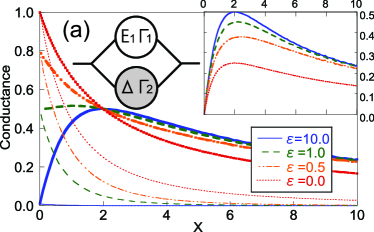
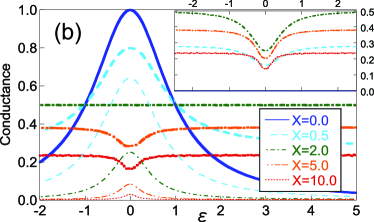
Figure 1: (Color Online) Conductance vs $X=\pi\Gamma_{2}/\Delta$ (a) and $\epsilon=(E-E_{1})/\Gamma_{1}$ (b) at $a=0$. The thick (thin) lines are the total conductance $g$ (the principal part $g_{0}$). Upper left inset in (a): Sketch of the sample. The parameters characterizing each dot are shown in the figure. Upper right inset in (a) and (b): Fluctuation part $\delta g=g-g_{0}$.

First we consider the $X$ dependence of the conductance at $a=0$. When $\epsilon\to\infty$, where the regular dot is detached from the random dot, we have $T_{1}=T_{2}=2X/(1+X/2)^{2}$, and recover the known result Efetov2

$$g_{0}=0,\quad\delta g=\frac{T_{1}}{3}+\frac{T_{1}^{2}}{6}.$$ (11)

At the resonance point $\epsilon=0$, $T_{1}=2X/(1+X/2)^{2}$, $T_{2}=0$, and we obtain

$$g_{0}=\frac{1}{\left(1+X/2\right)^{2}},\quad\delta g=\frac{T_{1}}{4}=\frac{X/2}{\left(1+X/2\right)^{2}}.$$ (12)

In Fig. 1(a), $X$ dependence of the conductance is shown for several values of $\epsilon$. $g_{0}$ shows a peak at $X=0$ while $\delta g$ takes a maximum at $X=2$, as shown by the thin lines and the inset in Fig. 1(a), respectively. As $\epsilon\to\infty$ $g_{0}$ ($\delta g$) is monotonically decreasing (increasing) and the result rapidly approaches Eq.(11).

$\epsilon$ dependence of the conductance is shown in Fig. 1(b). A resonance peak appears at $\epsilon=0$, reflecting transport through the regular dot. This peak structure, however, changes qualitatively as a function of $X$. For small $X$ the peak is convex and the peak height decreases on increasing $X$. When $X=2$, $g$ is independent of $\epsilon$. Increasing $X$ further, we find that the peak turns into an antiresonance and $g$ decreases monotonically. The result for $X=2$ corresponds to that of the CUE because $\langle S_{2}\rangle=0$, and the Poisson kernel $P(S_{2})$ becomes unity.

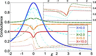
Figure 2: (Color Online) Conductance vs $\epsilon$ at $a=0.7$ and $\varphi=\pi/8$. The thick (thin) lines are the total conductance $g$ (principal part $g_{0}$). Inset: Fluctuation part $\delta g$.

The obtained results are for a model with a resonance at $a=0$. Now the question is whether they are characteristic of the resonance model. For comparison, we discuss the direct reaction model with $a\neq 0$ and $\epsilon\to\infty$. Both models are similar in that the conductance $g_{0}$ becomes finite in the absence of fluctuations. $g_{0}$ becomes maximum at $a=1$, which is similar to the situation at $\epsilon=0$ in the resonance model. In the direct reaction model, the eigenvalues of the $T$ matrix are given by

$$T_{1,2}=\frac{2(1\pm a)X}{\left[1+(1\pm a)X/2\right]^{2}}.$$ (13)

$T_{2}$ goes to zero as $a\to 1$ as in the limit $\epsilon\to 0$ in Eq.(9). In this limit, we find $T_{1}=4X/(1+X)^{2}$, $T_{2}=0$, and

$$g_{0}=\frac{X^{2}}{\left(1+X\right)^{2}},\quad\delta g=\frac{T_{1}}{4}=\frac{X}{\left(1+X\right)^{2}}.$$ (14)

Note that $T_{1}$ dependence of $\delta g$ is the same as in Eq.(12) but the $X$ dependence is different. We have found numerically that the peak is maintained for an arbitrary value of $X$ and that there is no antiresonance, in contrast to the resonance model.

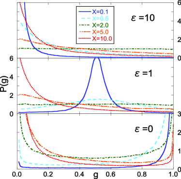
Figure 3: (Color Online) Conductance distribution at $a=0$.

As we have shown in Eq.(7), when we consider both the resonance and direct reaction channels, the Fano effect appears in $g_{0}$. In Fig. 2, a typical numerical result of the conductance is shown at $a=0.7$ and $\varphi=\pi/8$. We observe that an asymmetric form is obtained for the fluctuation part as well as for the principal part. However, these asymmetric peaks work to compensate each other, resulting in a symmetric $g$ that has a form similar to the previous result at $a=0$. The difference is that the conductance as a whole is enhanced due to the direct path contribution. Far from the resonance point, the conductance is independent of $\varphi$, while it is sensitive at the resonance point. The resonance (antiresonance) is amplified at $\varphi=0$ ($\pi/4$) where the Fano parameter $q$ is pure imaginary (real). When $q$ takes a complex value (when $0<\varphi<\pi/4$), a dip in the resonance peak is formed at the intermediate values of $X$ (See the plot of $X=2$ in Fig. 2).

As we have shown, $\delta g$ are of the order of $g_{0}$ and the mere calculation of the averaged conductance is not enough to characterize the system. We show the numerical results for the conductance distribution function $P(g)=\langle\delta(g-|S_{12}|^{2})\rangle$ in Fig. 3. For $\epsilon\gg 1$ we find the results in Refs. PEI, and randomS, expressed in terms of $T_{1}$ in Eq.(9). For finite value of $\epsilon$, the $T$ universality does not hold and the results essentially depend on $X$ and $\epsilon$. When $X<2$, the peak representing the resonant conductance moves from $g=0$ to 1 as $\epsilon$ decreases. When $X>2$, the resonant conductance is suppressed and the distribution function shows the strong influence of the chaotic scattering. When $\epsilon=0$, two peaks appear at $g=0$ and $1$. The peak at $g=0$ is larger (smaller) than that at $g=1$ when $X>2$ ($X<2$), which clearly shows the coexistence of the contributions from both regular and chaotic dots. At $X=2$, $P(g)$ is always symmetric and is consistent with the results of the averaged conductance. The curve for $\epsilon=0$ is well fitted by the function $P(g)=1/\pi\sqrt{g(1-g)}$.

We remark on the effect of dephasing. It can be simply studied by introducing an imaginary part to the energy $E\to E+i/2\tau$. The substitution of this to Eq.(7) leads to the reduction of the conductance. The effect on the fluctuation part is to add $F_{\tau}=(\Delta\tau)^{-1}\mbox{str}\,\sigma\Lambda$ to the $\sigma$ model. Numerically we have observed that the fluctuation part is strongly suppressed by this effect while the principal part shows a small reduction. This means that the resonance is preserved at any $X$. We also anticipate that an asymmetric Fano resonance can be observed, since the cancellation of the asymmetry between the principal and fluctuation parts becomes incomplete. The quantitative estimate of the dephasing effects using the method in Ref. BB, is necessary to compare with the experimental results, as was done in Refs. HPMBDH, and HZOAA, for the single–dot systems. A detailed study will be reported elsewhere.

Another interesting problem is the ensemble dependence of the result. Our numerical calculations using the orthogonal and symplectic ensembles show that the distribution at the resonant point (the lowest graph in Fig. 3) is independent of the ensemble. It implies the distribution is determined by some universal mechanism.

In conclusion, we have developed a statistical theory for an AB ring system with regular and chaotic QDs. The conductance and its distribution are strongly influenced by the mesoscopic fluctuations of the chaotic dot and the position of the resonance peaks.

We are grateful to A. Furusaki and S. Iida for useful discussions. T.A. acknowledges support from the Japan Society for the Promotion of Science.

References

- (1) C.W.J. Beenakker, Rev. Mod. Phys. 69, 731 (1997).
- (2) Y. Alhassid, Rev. Mod. Phys. 72, 895 (2000).
- (3) P.G. Silvestrov and Y. Imry, Phys. Rev. Lett. 85, 2565 (2000).
- (4) U. Fano, Phys. Rev. 124, 1866 (1961).
- (5) K. Kobayashi, H. Aikawa, S. Katsumoto, and Y. Iye, Phys. Rev. Lett. 88, 256806 (2002); Phys. Rev. B 68, 235304 (2003).
- (6) A.C. Johnson, C.M. Marcus, M.P. Hanson, and A.C. Gossard, Phys. Rev. Lett. 93, 106803 (2004).
- (7) S. Rotter, F. Libisch, J. Burgdörfer, U. Kuhl, and H.-J. Stöckmann, Phys. Rev. E 69, 046208 (2004).
- (8) J. Faist, F. Capasso, C. Sirtori, K.W. West, and L.N. Pfeiffer, Nature (London) 390, 589 (1997).
- (9) V.N. Prigodin, K.B. Efetov, and S. Iida, Phys. Rev. Lett. 71, 1230 (1993); Phys. Rev. B 51, 17223 (1995).
- (10) A.G. Huibers, S.R. Patel, C.M. Marcus, P.W. Brouwer, C.I. Duruöz, and J.S. Harris, Jr., Phys. Rev. Lett. 81, 1917 (1998).
- (11) S. Hemmady, X. Zheng, E. Ott, T.M. Antonsen, and S.M. Anlage, Phys. Rev. Lett. 94, 014102 (2005); S. Hemmady, X. Zheng, J. Hart, T.M. Antonsen, Jr., E. Ott, and S.M. Anlage, cond-mat/0512131 (unpublished).
- (12) A.A. Clerk, X. Waintal, and P.W. Brouwer, Phys. Rev. Lett. 86, 4636 (2001).
- (13) M.L. Mehta, Random Matrices (Academic Press, New York, 2004).
- (14) J.J.M. Verbaarschot, H.A. Weidenmüller, and M.R. Zirnbauer, Phys. Rep. 129, 367 (1985).
- (15) Y. Gefen, Y. Imry, and M.Ya. Azbel, Phys. Rev. Lett. 52, 129 (1984); B. Kubala and J. König, Phys. Rev. B 65, 245301 (2002); 67, 205303 (2003).
- (16) K.B. Efetov, Adv. Phys. 32, 53 (1983); Supersymmetry in Disorder and Chaos (Cambridge University Press, Cambridge, U.K., 1997).
- (17) H.U. Baranger and P.A. Mello, Phys. Rev. Lett. 73, 142 (1994); R.A. Jalabert, J.-L. Pichard, and C.W.J. Beenakker, Europhys. Lett. 27, 255 (1994); P.W. Brouwer and C.W.J. Beenakker, Phys. Rev. B 50, R11263 (1994).
- (18) L.K. Hua, Harmonic Analysis of Functions of Several Complex Variables in the Classical Domains (AMS, Providence, RI, 1963); P.A. Mello, P. Pereyra, and T.H. Seligman, Ann. Phys. (NY) 161, 254 (1985); see also Ref. Beenakker, .
- (19) P.W. Brouwer, Phys. Rev. B 51, 16878 (1995).
- (20) K.B. Efetov, Phys. Rev. Lett. 74, 2299 (1995).
- (21) P.W. Brouwer and C.W.J. Beenakker, Phys. Rev. B 55, 4695 (1997).