Alignment of Rods and Partition of Integers

Abstract

We study dynamical ordering of rods. In this process, rod alignment via pairwise interactions competes with diffusive wiggling. Under strong diffusion, the system is disordered, but at weak diffusion, the system is ordered. We present an exact steady-state solution for the nonlinear and nonlocal kinetic theory of this process. We find the Fourier transform as a function of the order parameter, and show that Fourier modes decay exponentially with the wave number. We also obtain the order parameter in terms of the diffusion constant. This solution is obtained using iterated partitions of the integer numbers.

I Introduction

Phase transitions from an isotropic, disordered state to a nematic, ordered state are fundamental in equilibrium statistical physics hes . They occur in liquid crystals cl ; dgp , complex fluids sas , and are closely related to phase synchronization yk ; shs ; abprs . The standard approach for describing order-disorder phase transitions is based on a Hamiltonian description. However, it may not necessarily apply in nonequilibrium settings such as granular systems bdve ; bnk ; at1 , where a non-equilibrium approach, that is based on kinetic interaction rules, may be required.

We study dynamical alignment of rods and show that the corresponding kinetic theory framework is appropriate for describing the underlying order-disorder phase transition. This approach conveniently allows characterization of statistical properties such as the distribution of rod orientation.

We consider the mean-field theory for alignment of interacting polar rods, introduced recently as a model at for ordering of microtubules by molecular motors in a planar geometry umamk ; nsml ; lk ; kjjps ; lm ; SS . In this model, rods become aligned by pairwise interactions, and they may also wiggle in a diffusive fashion, the latter process being governed by a white noise. This system reaches a steady-state where alignment by interactions is balanced by diffusion. With strong diffusion, the system is disordered, but with weak diffusion, the system becomes ordered.

Our main result is an exact steady-state solution for this kinetic theory. The Fourier modes obey a closed set of coupled nonlinear equations. By iterating these equations, it is possible to relate all Fourier modes to the lowest mode, which in turn is equivalent to the order parameter. Similarly, the order parameter itself is shown to obey a closed equation and this allows one to express the distribution of rod orientations in terms of the diffusion constant. While in principle, the complete solution involves an infinite number of Fourier modes, in practice, it is sufficient to consider only a moderate number of modes because the Fourier modes decay exponentially with the wave number.

The exact solution is ultimately related to iterated partitions of the integers numbers. This feature is generic: it applies to general alignment rules, as well as to arbitrary alignment rates. We also find that depending on the alignment rate, the system may or may not undergo a phase transition.

This paper is organized as follows. In Sect. II, we describe the rod alignment model. In Sect. III, we perform the Fourier transform of the governing equation, which is then solved in Sect. IV. We discuss nearly perfect alignment in Sect. V, and briefly mention several generalizations in Sect. VI. We conclude in Section VII.

II The Rod Alignment Model

In the rod alignment model, introduced by Aranson and Tsimring at , there is an infinite number of identical polar rods, each with an orientation $-\pi\leq\theta\leq\pi$. The rods become aligned via irreversible pairwise interactions. As a result of the interaction between two rods with orientations $\theta_{1}$ and $\theta_{2}$, both rods acquire the average orientation as follows (see also figure 1):

$$(\theta_{1},\theta_{2})\to\begin{cases}\left(\frac{\theta_{1}+\theta_{2}}{2},\frac{\theta_{1}+\theta_{2}}{2}\right)&|\theta_{1}-\theta_{2}|<\pi\\ \left(\frac{\theta_{1}+\theta_{2}+2\pi}{2},\frac{\theta_{1}+\theta_{2}+2\pi}{2}\right)&|\theta_{1}-\theta_{2}|>\pi.\end{cases}$$ (1)

Here, and throughout this study, addition and subtraction are implicitly taken modulo $2\pi$.

Figure 1: Illustrating of the alignment process.

There is also randomness in the form of a white noise: each rod wiggles in a diffusive fashion, and this process is characterized by the diffusion constant $D$. Specifically, in addition to the alignment process (1), the orientation of a rod changes according to $d\theta/dt=\eta$ with $\eta$ an uncorrelated white noise $\langle\eta(t)\eta(t^{\prime})\rangle=2D\delta(t-t^{\prime})$.

Let $P(\theta,t)$ be the probability distribution function of rods with orientation $\theta$ at time $t$. It is normalized to one, $\int_{-\pi}^{\pi}d\theta\,P(\theta,t)=1$. This distribution function satisfies the integro-differential master equation

$$\frac{\partial P}{\partial t}=D\frac{\partial^{2}P}{\partial\theta^{2}}+\int_{-\pi}^{\pi}d\phi\,P\left(\theta-\frac{\phi}{2}\right)P\left(\theta+\frac{\phi}{2}\right)-P.$$ (2)

The first term on the right-hand-side describes diffusion. The integral accounts for gain of rods with orientation $\theta$ as a result of alignment of two rods with an orientation difference of $\phi$, while the negative term accounts for loss due to alignment. Without loss of generality, the alignment rate is set to $1/2$ so that the loss rate equals one. This kinetic theory generalizes the Maxwell model of inelastic collisions in a granular gas as all rods interact with each other and additionally, the alignment rate is independent of the relative orientation bk1 ; bk2 .

III The Fourier Transform

The governing master equation (2) is nonlinear and nonlocal. Its convolution structure suggests using the Fourier transform

$$P_{k}=\big{\langle}e^{-ik\theta}\big{\rangle}=\int_{-\pi}^{\pi}d\theta\,e^{-ik\theta}\,P(\theta).$$ (3)

The zeroth mode equals one, $P_{0}=1$, because of the normalization, and also, $P_{k}=P_{-k}^{*}$. The angular distribution can be expressed as a Fourier series

$$P(\theta)=\frac{1}{2\pi}\sum_{k=-\infty}^{\infty}P_{k}\,e^{ik\theta}.$$ (4)

Since the alignment process (1) is invariant with respect to an overall rotation $\theta\to\theta+\varphi$ with an arbitrary phase $0\leq\varphi\leq 2\pi$, if $P(\theta)$ and $P_{k}$ are solutions of (2), then so are $P(\theta+\varphi)$ and $P_{k}e^{ik\varphi}$, respectively.

The order parameter $R=\big{|}\langle e^{i\theta}\rangle\big{|}=\left|P_{-1}\right|$, with the bounds $0\leq R\leq 1$ probes the state of the system. A vanishing order parameter indicates an isotropic, disordered state, while a positive order parameter reflects a nematic, ordered state.

We focus on the steady state. Substituting the Fourier series (4) into the master equation (2), setting $\partial P/\partial t\equiv 0$, and integrating over $\phi$, we find that the Fourier transform satisfies a set of coupled nonlinear equations at

$$\left(1+Dk^{2}\right)P_{k}=\sum_{i+j=k}A_{i-j}\,P_{i}\,P_{j},$$ (5)

with $A_{q}=\frac{1}{2\pi}\int_{-\pi}^{\pi}d\phi\,e^{iq\phi/2}=\frac{\sin\pi q/2}{\pi q/2}$. The coefficients $A_{q}$ are symmetric, $A_{q}=A_{-q}$, and explicitly,

$$A_{q}=\begin{cases}1&q=0;\\ 0&|q|=2,4,\ldots;\\ (-1)^{\frac{q-1}{2}}\frac{2}{\pi|q|}&|q|=1,3,\ldots\end{cases}$$ (6)

In (5), when $k=0$, the sum contains only a single term, $P_{0}=P_{0}^{2}$ and indeed, $P_{0}=1$.

Since $P_{0}=1$ is known, the identical terms $A_{-k}P_{0}P_{k}$ and $A_{k}P_{k}P_{0}$ in the steady-state equation (5) are linear in $P_{k}$, and thus, we move them to the left-hand side. Then Eq. (5) becomes

$$\left(1+Dk^{2}-2A_{k}\right)\,P_{k}=\sum_{\begin{subarray}{c}i+j=k\\ i\neq 0,\,j\neq 0\end{subarray}}A_{i-j}\,P_{i}\,P_{j}.$$ (7)

Next, we absorb the prefactor on the left-hand side into the kernel on the right-hand side by introducing the rescaled kernel

$$G_{i,j}=\frac{A_{i-j}}{1+D(i+j)^{2}-2A_{i+j}}.$$ (8)

With this transformation, we arrive at a compact, and simpler-to-analyze, equation for the steady-state Fourier transform

$$P_{k}=\sum_{\begin{subarray}{c}i+j=k\\ i\neq 0,\,j\neq 0\end{subarray}}G_{i,j}P_{i}\,P_{j}.$$ (9)

The kernel $G_{i,j}$ couples the $i$th and the $j$th Fourier modes. It has the following properties:

$$G_{i,j} =G_{j,i},$$ (10a)

$$G_{i,j} =G_{-i,-j},$$ (10b)

$$G_{i,j} =0,\qquad{\rm for}\qquad|i-j|=2,4,\ldots.$$ (10c)

The governing equation (9) is nonlinear and moreover, for odd $k$, the sum contains an infinite number of terms. Despite this, it is still possible to solve this equation analytically!

IV Exact Solution

First, we notice that Eq. (9) can be iterated once, leading to a sum of products of three Fourier modes

$$P_{k}=\sum_{\begin{subarray}{c}i+j=k\\ i\neq 0,\,j\neq 0\end{subarray}}\sum_{\begin{subarray}{c}l+m=j\\ l\neq 0,\,m\neq 0\end{subarray}}G_{i,j}G_{l,m}\,P_{i}\,P_{l}\,P_{m}.$$ (11)

Clearly, this procedure can be repeated any number of times, leading to a sum over products of any given number of Fourier modes.

Using this iteration procedure for all but the lowest Fourier mode, it is possible to express $P_{k}$ as an explicit function of $P_{\pm 1}$ only. For instance, when $k=2$, Eq. (9) is simply $P_{2}=G_{1,1}P_{1}^{2}$ and when $k=4$ one has $P_{4}=G_{2,2}P_{2}^{2}$. Thus, the fourth Fourier mode is also expressed in terms of the lowest mode, $P_{4}=G_{2,2}G_{1,1}^{2}P_{1}^{4}$ note . Odd modes, in contrast, involve an infinite sum. For the third mode, $P_{3}=2G_{1,2}P_{1}P_{2}+2G_{-1,4}P_{-1}P_{4}+\cdots$, and substituting the second and the fourth moments above,

$$P_{3}=2G_{1,2}G_{1,1}P_{1}^{3}+2G_{-1,4}G_{2,2}G_{1,1}^{2}P_{1}^{4}P_{-1}+\cdots.$$

Generally, the $k$th Fourier mode can be written as an infinite series involving terms of the form

$$P_{1}^{k+n}P_{-1}^{n}=P_{1}^{k}(P_{1}\,P_{-1})^{n}=P_{1}^{k}R^{2n}$$

with $n$ a positive integer. Recall that $P_{1}=R\,e^{i\varphi}$. Without loss of generality, we can set the phase to zero, $\varphi=0$. Then $P_{1}=R$ and the Fourier modes can be written explicitly in terms of the order parameter $R$

$$P_{k}=R^{k}\,\sum_{n=0}^{\infty}\,p_{k,n}\,R^{2n}.$$ (12)

Of course, $p_{0,n}=p_{\pm 1,n}=\delta_{n,0}$. Since $p_{k,n}=p_{-k,n}$ it suffices to solve for $k>0$.

The coefficients $p_{k,n}$ represent all iterated partitions of the integer $k$ as follows

$$k=\underbrace{1+1+\cdots+1+1}_{k+n}\underbrace{-1-\cdots-1}_{n}.$$ (13)

The iterated partition involves a series of integer partitions $k=i+j$, subject to the following restrictions: (i) $i\neq 0$ and $j\neq 0$, (ii) $|k|\neq 1$, (iii) $G_{i,j}\neq 0$. Each such partition contributes a factor $G_{ij}$ to $p_{k,n}$ (figure 2). For example, the partition $2=(1+1)$ gives $p_{2,0}=G_{1,1}$ and the two equivalent partitions $3=(1+2)=(1+(1+1))$ and $3=(2+1)=((1+1)+1)$ give $p_{3,0}=2G_{1,2}G_{1,1}$. We list all non-vanishing terms up to the fifth order in $R$

$$p_{2,0} =G_{1,1},$$ (14a)

$$p_{3,0} =2G_{1,2}G_{1,1},$$ (14b)

$$p_{3,1} =2G_{-1,4}G_{2,2}G^{2}_{1,1},$$ (14c)

$$p_{4,0} =G_{2,2}G^{2}_{1,1},$$ (14d)

$$p_{5,0} =2G_{1,4}G_{2,2}G^{2}_{1,1}+4G_{2,3}G_{1,2}G^{2}_{1,1}.$$ (14e)

Here, we used the symmetries (10a) and (10b) to consolidate identical terms. We stress that the partitions used here differ from traditional integer partitions in that they involve negative integers and in that they are iterated ae .

Substituting the series expansion (12) into the steady-state equation (9) and equating the same powers of $R$, the coefficients $p_{k,n}$ satisfy

$$p_{k,n}=\sum_{l+m=n}\sum_{\begin{subarray}{c}i+j=k\\ i\neq 0,\,j\neq 0\end{subarray}}p_{i,l}\,p_{j,m}.$$ (15)

Since the indexes $l$ and $m$ are positive, this is now a recursion equation. Starting with $p_{0,0}=p_{1,0}=1$, and utilizing the symmetry $p_{k,n}=p_{-k,n}$, equation (15) is solved recursively. This provides a systematic method for obtaining the coefficients $p_{k,n}$.

Figure 2: The iterated integer partitions. Illustrated is the partition corresponding to $p_{3,1}=2G_{-1,4}G_{2,2}G^{2}_{1,1}$. Each partition $k=i+j$ with $i\neq 0$ and $j\neq 0$ generates a factor $G_{i,j}$. The factor 2 accounts for the two equivalent partitions.

The series (12) expresses all the Fourier modes in terms of the order parameter $R$. It remains to obtain the order parameter $R$ as a function of the diffusion constant $D$. By Substituting the Fourier solution (12) into the governing equation (9) and setting $k=1$, we find that the order parameter itself can be expressed as an infinite series

$$R=\sum_{n=1}^{\infty}r_{n}R^{2n+1}.$$ (16)

The coefficients $r_{n}$ are given by the very same recursion equation (15)

$$r_{n}=\sum_{l+m=n}\sum_{\begin{subarray}{c}i+j=1\\ i\neq 0,\,j\neq 0\end{subarray}}\,p_{i,l}\,p_{j,m}.$$ (17)

The coefficient $r_{n}$ is the counterpart of the coefficients $p_{k,n}$ and it represents iterated partitions of the number $1$ as in (13). The partitions may not involve $0$’s. Except for the very first partition, the numbers $\pm 1$ may not be repartitioned (Fig. 2). The first few coefficients are

$$r_{1} =2G_{-1,2}G_{1,1},$$ (18a)

$$r_{2} =4G_{-2,3}G_{1,2}G^{2}_{1,1},$$ (18b)

$$r_{3} =4(G_{-2,3}G_{-1,4}+G_{-3,4}G_{1,2})G_{2,2}G_{1,1}^{3}.$$ (18c)

Equation (16) is a closed equation for the order parameter. Once it is solved, all Fourier modes follow from (12). This completes the solution for $R$ and $P_{k}$, and therefore for the angle distribution $P(\theta)$.

In practice, one can calculate the order parameter $R$ as a root of a polynomial of degree $N$ by truncating (16). For $N=3$, substituting (6) and (8) into (18a) yields $r_{1}=-\frac{4}{3\pi}(1+D-4/\pi)^{-1}(1+4D)^{-1}$, and using (16) gives the cubic equation for the order parameter

$$R=\frac{4}{3\pi}\frac{1}{D_{c}-D}\frac{1}{1+4D}R^{3},$$ (19)

with the critical diffusion constant

$$D_{c}=\frac{4}{\pi}-1.$$ (20)

For $D\geq D_{c}$, there is only the trivial solution $R=0$, corresponding to an isotropic state where the rods are randomly aligned: $P_{k}=\delta_{k,0}$ and $P(\theta)=\frac{1}{2\pi}$. Below the critical point, $D<D_{c}$, there is also the nontrivial solution (Fig. 3)

$$R=\sqrt{\frac{3\pi}{4}(1+4D)(D_{c}-D)}.$$ (21)

This corresponds to a nematic phase in which the rods are partially aligned. Near the transition point, this alignment is weak, but it becomes stronger and stronger as $D$ decreases. The result of Eq. (21) is approximate—only the cubic term in (16) has been maintained—yet sufficiently close to the transition point, the corrections to the cubic equation (19) are negligible and $R\simeq C(D_{c}-D)^{\beta}$ with the prefactor $C=\sqrt{(3/4)(16-3\pi)}$ and the mean-field exponent $\beta=1/2$ hes ; yk ; at is asymptotically exact. As shown in the Appendix, the uniform state is stable for $D>D_{c}$ but unstable for $D<D_{c}$.

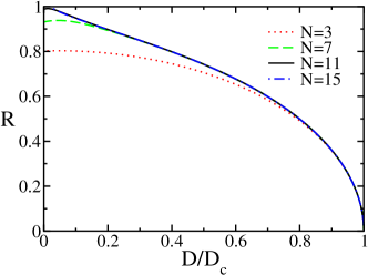
Figure 3: The order parameter versus the diffusion coefficient. The order parameter was obtained by solving polynomials of increasing order.

Well below the critical point, we compute the coefficients $p_{k,n}$ and $r_{n}$ to higher order from (15) and (17). The order parameter is then obtained by numerically solving (16), truncated at the corresponding order. Since the Fourier modes decay exponentially with the wave number

$$P_{k}\sim R^{k},$$ (22)

and since the order parameter obeys $0\leq R\leq 1$, a moderate number of Fourier modes is sufficient to accurately compute $P(\theta)$. The order parameter rapidly converges with $N$. For instance, $N=11$ already provided an accurate value for $R$ (see Fig. 3). We note that at this order, it is still possible to calculate the necessary partitions manually.

Once the order parameter is known, the Fourier modes are obtained from (12). The steady-state distribution (4) becomes

$$P(\theta) = \frac{1}{2\pi}+\frac{1}{\pi}\,R\cos\theta+\frac{1}{\pi}G_{1,1}R^{2}\cos\,(2\theta)$$

$$+ \frac{2}{\pi}G_{1,2}G_{1,1}R^{3}\cos\,(3\theta)+O(R^{4}).$$

In the vicinity of the transition point, the lowest mode dominates. As the diffusion coefficient decreases, the angle distribution becomes sharply peaked around $\theta=0$, reflecting that the rods are strongly aligned (Fig. 4). We now analyze this nearly perfect alignment in more detail.

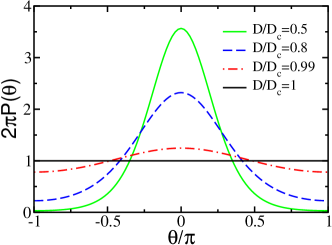
Figure 4: The angular distribution for various values of $D$. The angle distribution was obtained from the first 15 Fourier modes.

V Nearly perfect alignment

For very small diffusion constants, the order parameter approaches unity and therefore, the series solution (12) is no longer useful. Indeed, very close to $D=0$, the convergence is slow (Fig. 3). Nevertheless, it is still possible to treat the problem by performing the scaling transformation

$$P(\theta)=\frac{1}{\sqrt{D}}f\left(\frac{\theta}{\sqrt{D}}\right).$$ (24)

The scaling distribution remains normalized, $\int dxf(x)=1$. At the steady-state, it obeys the nonlinear integro-differential equation

$$f(x)=\frac{d^{2}f(x)}{dx^{2}}+\int_{-\infty}^{\infty}dy\,f\left(x-\frac{y}{2}\right)f\left(x+\frac{y}{2}\right).$$ (25)

This equation was obtained by substituting (24) into the master equation (2), setting the time derivative to zero, and replacing the integration limits $\pm\pi/\sqrt{D}$ with $\infty$. In the limit $D\to 0$, the periodic nature becomes irrelevant, and the problem reduces to the randomly forced inelastic Maxwell model, for which several properties including the moments and the Fourier transform can be obtained analytically bk1 ; bk2 .

Consider for example the normalized moments $M_{n}=\langle\theta^{n}\rangle/n!$. They can be expressed in terms of the moments of the scaling distribution $M_{n}=D^{n/2}m_{n}$ with $m_{n}=\int dx\,x^{n}f(x)/n!$. Substituting this definition into the master equation (25) and performing the integration, the moments $m_{n}$ satisfy the closed set of equations $m_{n}=m_{n-2}+2^{-n}\sum_{l=0}^{n}m_{l}\,m_{n-l}$, from which the moments are found recursively, $m_{0}=1$, $m_{2}=2$, and $m_{4}=\frac{18}{7}$ (the odd moments vanish). The order parameter can be expressed in terms of the moments, $R=\big{|}\langle e^{i\theta}\rangle\big{|}=1-M_{2}+M_{4}+\cdots$ and therefore, it is given by a Taylor series in powers of the diffusion constant

$$R=1-2D+\frac{18}{7}D^{2}+\cdots.$$ (26)

This expression is useful only for very small diffusion constants, i.e., $D\to 0$.

Since the Fourier transform $F(q)=\int_{-\infty}^{\infty}dx\,e^{iqx}f(x)$ is the generating function of the moments, it also satisfies a closed equation, $\left(1+q^{2}\right)F(q)=F^{2}\left(q/2\right)$. Solving this equation recursively, the Fourier transform equals the infinite product bk1

$$F(q)=\prod_{n=0}^{\infty}\left[1+\frac{q^{2}}{4^{n}}\right]^{-2^{n}}.$$ (27)

The poles closest to the origin govern the large-$x$ asymptotics. The simple poles located at $q=\pm i$ imply an exponential decay bk2 ; se ; adl

$$f(x)\simeq Ce^{-|x|}$$ (28)

as $|x|\to\infty$. The residues to these poles yield the prefactor: $C=\frac{1}{2}\,\exp\left[\sum_{n=1}^{\infty}n^{-1}(2^{2n-1}-1)^{-1}\right]=1.47919$.

VI General Alignment Rates

The above solution can be generalized in a number of ways. For instance, it is straightforward to generalize it to imperfect alignment processes, where the orientation difference is reduced by a fixed factor (analogous to an imperfect inelastic collision), in each alignment event.

Moreover, it is also possible to analyze situations in which the alignment process (1) occurs with arbitrary alignment rate $K\big{(}\theta_{1}-\theta_{2})$. We assume $K(\phi)=K(-\phi)$ and without loss of generality, impose the normalization, $\frac{1}{2\pi}\int_{-\pi}^{\pi}d\phi\,K(\phi)=1$. The master equation becomes

$$0 = D\frac{d^{2}P}{d\theta^{2}}+\int_{-\pi}^{\pi}d\phi\,K(\phi)P\left(\theta-\frac{\phi}{2}\right)P\left(\theta+\frac{\phi}{2}\right)$$ (29)

$$- P(\theta)\int_{-\pi}^{\pi}d\phi\,K(\phi)P(\theta+\phi).$$

The Fourier modes satisfy a generalization of (5)

$$Dk^{2}P_{k}=\frac{1}{2}\sum_{i+j=k}(A_{i-j}+A_{j-i}-A_{2i}-A_{2j})\,P_{i}P_{j}.$$ (30)

The constant $A_{q}$ is now $A_{q}=\frac{1}{2\pi}\int_{-\pi}^{\pi}d\phi\,e^{iq\phi/2}K(\phi)$. Again $A_{0}=1$ and $A_{q}=A_{-q}$, but it is not necessarily true that these constants vanish at even indexes as was the case for uniform alignment rates. By excluding the zero modes $i=0$ and $j=0$ from the summation in (30), and by following the same steps, we recover the governing steady-state Eq. (9). The generalized coupling constants (8) are

$$G_{i,j}=\frac{1}{2}\frac{A_{i-j}+A_{j-i}-A_{2i}-A_{2j}}{1+D(i+j)^{2}-2A_{i+j}}.$$ (31)

These coupling constants are manifestly symmetric $G_{i,j}=G_{j,i}$. We conclude that the series solutions (12) and (16) hold for arbitrary alignment rates.

By repeating the steps leading to (20), we find that the critical diffusivity generally equals $D_{c}=2A_{1}-1$. The condition for having a transition is therefore $A_{1}>1/2$. For the constant interaction rate $A_{1}=\frac{2}{\pi}$, and then $D_{c}=\frac{4}{\pi}-1$. For the hard-sphere rate $K(\phi)=\frac{2}{\pi}|\phi|$, then $A_{1}=\frac{4}{\pi^{2}}(2-\pi)$, but since $A_{1}<1/2$, the system is always disordered. Therefore, depending on the alignment rate, there may or may not be an ordered phase.

We note that in the kinetic theory of gases, analytic solutions are feasible only for the Maxwell model, where the collision rate is velocity independent max ; classical ; e , while the general Boltzmann equation is not analytically tractable. Remarkably, the analytic solution presented above does not require a constant rate and for example, the hard-sphere like collision rate $K(\phi)=C|\phi|$ can be solved analytically. The discrete nature of the Fourier spectrum makes this possible.

VII Conclusions

In conclusion, we studied kinetic theory for alignment of rods. At the steady-state, alignment by pairwise interactions is balanced by the diffusive motion. At large diffusivities, the system is disordered and at low diffusivities it becomes ordered.

The Fourier modes obey a closed equation that can be solved by selective iterations. This allows one to express all Fourier modes in terms of the lowest mode, or equivalently, the order parameter. Similarly, one can obtain a closed equation for the order parameter itself, and then the solution becomes explicit. Since the Fourier modes decay exponentially with the wave number, a moderate number of terms is sufficient to accurately obtain the full angular distribution.

This kinetic approach fundamentally differs from the traditional Hamiltonian approach for describing phase transitions from ordered to disordered states. Yet, the characteristics of the phase transition, including in particular, the critical exponent, are identical to the mean-field theory. The kinetic theory has the virtue that it directly yields distribution functions.

The exact solution, using integer partitions, is very general. It applies to generic “inelastic” alignment rules and more importantly, to general alignment rates. The periodic symmetry of the problem is ultimately responsible for this because it involves a discrete Fourier spectrum. It may be useful to generalize this approach to alignment of rods in three dimensions.

The nonlocal and nonlinear governing equation, in its simplest form (9), appears in other physical processes including aggregation fran , and it may be interesting to utilize the integer partition solution method in other contexts. There are other natural extensions of this work including investigation of relaxation toward the steady-state, studies of spatial correlations in low-dimensional systems, and restricted range interactions where multiple alignment directions may arise bkr ; plr .

Experimentally, it may be possible to realize this order-disorder transition by vibrating macroscopic granular chains bdve or granular rods bnk ; at1 where vibration causes diffusion and inelastic collisions result in alignment.

Appendix A Stability of the uniform state

The uniform state $P(\theta)=\frac{1}{2\pi}$ is always a steady-state of the master equation (2). To check when this state is stable, we write $P(\theta,t)=\frac{1}{2\pi}+p(\theta,t)$. To linear order, the perturbation satisfies

$$\frac{\partial p}{\partial t}=D\frac{\partial^{2}p}{\partial\theta^{2}}+\int_{-\pi}^{\pi}\!\!d\phi\,\frac{p(\theta-\phi/2)+p(\theta+\phi/2)}{2\pi}-p.$$ (32)

Let us take a periodic perturbation with wave number $k$ and growth rate $\lambda$, that is, $p(\theta,t)\propto e^{ik\theta+\lambda t}$. Substituting this form into Eq. (32) gives the growth rate

$$\lambda_{k}=2A_{k}-1-Dk^{2}.$$ (33)

The growth rate is positive only for the lowest mode, $k=1$, and hence, stability is governed by the smallest wave number $k=1$ for which $\lambda_{1}=D_{c}-D$. Indeed, the uniform state is unstable below the critical diffusion constant (20).