Decoherence and Quantum Measurement of Josephson-Junction Qubits

Abstract

This work deals with two pressing issues in the design and operation of Josephson qubits – loss of coherence and measurement.

The first part is devoted to the problem of decoherence in single and double qubit systems. We present a quantitative description of quantum coherent oscillations in the system of two coupled qubits in the presence of weak noise that in general can be correlated between the two qubits. It is shown that in the experimentally realized scheme the waveform of the excited oscillations is not very sensitive to the magnitude of decoherence correlations. Modification of this scheme into a potentially useful probe of the degree of decoherence correlations at the two qubits is suggested. Furthermore, an explicit non-perturbative expression for decoherence of quantum oscillations in a single and double qubit systems by low-frequency noise is presented. Decoherence strength is controlled by the noise spectral density at zero frequency while the noise correlation time $\tau$ determines the time $t$ of crossover from the $1/\sqrt{t}$ to the exponential suppression of coherence. The first part is concluded by introduction of a useful Monte-Carlo-based numerical technique for simulations of realistic qubit dynamics subject to general noise, time dependent bias and tunneling, and general environment temperature.

The second part addresses the problem of quantum measurement of qubit through discussion of a versatile new type of the magnetic flux detector which can be optimized to perform several measurement schemes in quantum-limited regime. The detector is based on manipulation of ballistic motion of individual fluxons in a Josephson transmission line (JTL), with the output information contained in either probabilities of fluxon transmission/reflection, or time delay associated with the fluxon propagation along the JTL. The equations for conditional evolution of the measured system both in the transmission/reflection and time-delay regimes are derived for this detector. Combination of the quantum-limited detection with control over individual fluxons should make the JTL detector suitable for implementation of non-trivial quantum measurement strategies, including conditional measurements and feedback control schemes.

To my parents and grandparents.

Chapter 1 Introduction

Any algorithmic process can be simulated efficiently (i.e. in polynomial time) using a Turing Machine is the celebrated Church-Turing thesis that for a long time instilled the belief that the efficiency of computation is independent of its underlying physical process [1, 2]. For this reason, the efficiency of computer architecture built on irreversible binary language was not questioned at first. Rather, one of the important topics in the earlier research of computational devices was the energy dissipation. One such study [3] showed that the erasure of information is the only source of energy dissipation. Later, it was suggested [4] that the fundamental limit of energy dissipation, $k_{B}Tln2$ per one erased bit of information, can be avoided by employing the computation that is both physically and logically reversible since reversible system can always be ”rolled back” to the zero state along constant energy path.

A particular way to employ reversible computation is by using quantum mechanics as the underlying physical process of computation since all closed quantum systems are reversible. In addition to the vanishing energy dissipation, a quantum system provides a possibility of preparing a superposition of its different states. This speeds up the information processing since it allows operating on many states of the computational basis simultaneously.

The advantage of this so-called quantum parallelism and the reversibility of quantum systems was for the first time fully realized by David Deutsch. He formulated quantum computation as a new field of computation based on quantum rather than classical dynamics [5]. The same work featured the first quantum algorithm that was in certain cases more efficient than any Turing machine algorithm for the same problem. In 1992 together with Jozsa, Deutsch improved on this algorithm so that it was always more efficient than any classical one [6]. Further discoveries of quantum algorithms that are more efficient than the respective classical algorithms by Simon [7], Shor [8], and Grover [9] propelled quantum computation into the forefront of scientific research.

The fundamental element of quantum computation is the quantum bit or qubit for short. It is a two-level unitary system where the unitarity is manifested through the presence of the quantum coherent oscillations. The oscillations represent periodically evolving probability of a qubit occupying some mixture of its two states. For this reason reconstructing previous states of the qubit is always possible. Decoherence, i.e. the loss of coherence, suppresses the quantum coherent oscillations and with it the reversibility of the qubit and in the process degrades its ability to preform the tasks needed in quantum computation [10].

An isolated quantum system does not exhibit decoherence. For it to happen, the quantum system needs to interact with other systems in a such way that its dynamics becomes dependent on the surrounding systems. Classical systems in such circumstances undergo energy relaxation as described by the fluctuation-dissipation theorem [11]. Quantum systems exhibit energy relaxation and decoherence. While quantum relaxation has its counterpart in classical dynamics, decoherence is a purely quantum phenomenon. It is caused by quantum phase interference or entanglement of two systems. It is not conditional on the systems being in contact all the time, rather if entangled in the past, the two systems generally stay entangled.

For computational purposes the qubit needs to be initialized, coupled with other qubits, and in the end measured. This requires entanglement of the qubit with the other qubits and the surroundings. Thus to have a qubit completely isolated from the environment is impossible. Rather, it is necessary to find ways to design physical qubits so that they exhibit prolonged coherent oscillations while integrated in larger structures.

The leading candidate for achieving such goals are superconducting Josephson junctions. They are scalable and integrable solid state devices where Cooper pairs of electrons move in phase and behave as a single quantum particle of much larger size than than the elementary quantum particles. Additionally Josephson junctions are ideal for nano-fabrication and integration into larger circuits needed for additional tasks such as measurement.

Measurement can be seen as an extraction of information from the computational device and its transcription into a classical signal. The rate of the information extraction from the qubit is at the most as fast as its rate of decoherence due to the back-action of the measuring device [12]. Furthermore, the ”no-cloning” theorem (eg. see [13]) prevents us from making multiple copies of the same qubit and repeating the same measurement to recover any lost information. Therefore, when devising the measurement of a qubit it is imperative to be as close as possible to this ideal limit, otherwise the non-ideal measurement of qubit will result in the loss of information.

We see that decoherence is present and measurement is needed in the design of quantum computers. Understanding these processes is imperative for the further advancement of the field.

1.1 Quantum Mechanics of a Two-Level System

We can think of a qubit as a quantum system where two of its neighboring levels with similar energies are separated by big energy gaps from the remaining levels, so that they can be considered independent. This can be accomplished with a mesoscopic Josephson junction consisting of a small superconducting island or a box separated by a thin insulating barrier from a larger superconducting electrode so that Cooper pairs can tunnel to and from the box [14, 15]. If the superconducting gap of the box is much larger than the thermal energy $k_{B}T$ and the charging energy of the box $E_{c}\equiv 2e^{2}/C$, then its dynamical properties are solely determined by the excess number of Cooper pairs in the box. The potential difference $V_{q}$ between the island and the electrode induces continuous polarization charge $CV_{q}$ inside the Cooper pair box of capacitance $C$. Because of the small size of the box, its capacitance is small, and the energy spectrum of the box is dominated by its charging energy. The quantum tunneling of Cooper pairs between the box and the reservoir is then a perturbative effect described by Josephson tunneling amplitude $-E_{J}/2$.

In the basis spanned by the number of Cooper pairs in the box $|n\rangle$, the Hamiltonian of the system consists of the charging and tunneling parts which in that order yield the Hamiltonian as:

$$H=E_{c}(n-n_{q})^{2}-\frac{E_{J}}{2}\left(|n\rangle\langle n+1|+|n+1\rangle\langle n|\right),$$ (1.1)

where $n$ is the excess number of the Cooper pairs in the box, and $n_{q}\equiv CV_{q}/2e$ is the induced static charge expressed as the number of Cooper pairs, $n_{q}\in[0,1)$. If the applied potential $V_{q}$ is adjusted that $n_{q}\approx 1/2$, the gap between the system’s two lowest charge states $|n=0\rangle\equiv|R\rangle$ and $|n=1\rangle\equiv|L\rangle$ is small (i.e. $E_{10}=E_{C}(1-2n_{q})\approx 0$), while the gap to the other states is on the order of $E_{C}$ and considerably larger. If $k_{B}T\ll E_{C}$, the two lowest levels are separated from the rest of the levels (figure 1.1a) and as experimentally demonstrated in [16, 17] they can be considered independent.

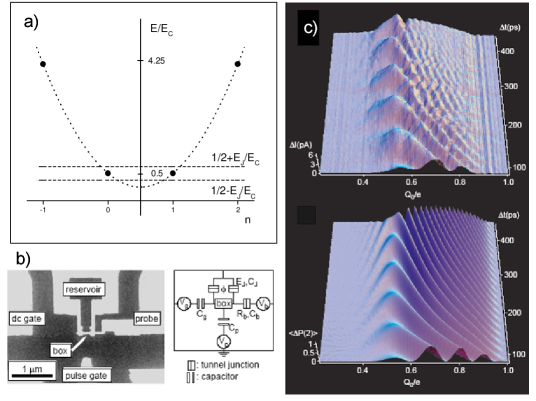
Figure 1.1: a) Energy spectrum of Josephson junction operating in charge regime with dots representing energy values of different charge states and dashed lines representing two lowest quantum levels with charging energy degeneracy removed by Josephson tunneling ($E_{C}/E_{J}=8,q=1/2$). b). Picture and scheme of the first operational charge qubit. c) The quantum coherent oscillations observed by Nakamura et. al. with the device pictured above [18]

.

After truncation of the higher energy levels, the Hamiltonian (1.1) can be written in the form of a general qubit Hamiltonian

$$H=-\frac{1}{2}(\varepsilon\sigma_{z}+\Delta\sigma_{x}),$$ (1.2)

where $\sigma_{x,z}$ are Pauli matrices, $\varepsilon=E_{C}(1-2n_{q})/2$, and $\Delta=|E_{J}|$ . The eigenvectors $|0\rangle$ and $|1\rangle$ of this Hamiltonian define the energy basis of the qubit with eigenenergies $\pm\Omega/2$. The qubit Hamiltonian is diagonal in this basis, $H_{diag}=-\Omega/2\>\sigma_{z}$, and the vectors spanning the two bases are related as

$$|L\rangle=x_{-}|0\rangle+x_{+}|1\rangle,\quad|R\rangle=x_{+}|0\rangle-x_{-}|1\rangle,$$ (1.3)

where $x_{\pm}=\sqrt{(\Omega\pm\varepsilon)/2\Omega}$ and $\Omega=\sqrt{\varepsilon^{2}+\Delta^{2}}$.

The state of the qubit is fully specified by its wave function $|\Psi(t)\rangle$, while its time evolution is determined by unitary transformation on $|\Psi\rangle$,

$$|\Psi(t)\rangle=\exp\left[-\frac{i}{\hbar}\int_{t_{0}}^{t}H(t^{\prime})dt^{\prime}\right]|\Psi(t_{0})\rangle.$$ (1.4)

Given the normalized wave function of the qubit as $|\Psi(0)\rangle=a|0\rangle+b|1\rangle$, in time $t$ it evolves to $|\Psi(t)\rangle=ae^{i\Omega t/2}|0\rangle+be^{-i\Omega t/2}|1\rangle$ expressed in the energy basis, or equivalently to

$$|\Psi(t)\rangle=\left(ax_{+}e^{i\Omega t/2}-bx_{-}e^{-i\Omega t/2}\right)|L\rangle+\left(ax_{-}e^{i\Omega t/2}+bx_{+}e^{-i\Omega t/2}\right)|R\rangle,$$ (1.5)

if expressed in the charge basis. As it can be seen above, the probability of finding the qubit in one of its eigenstates is stationary, while the probability of finding the qubit in one of its charge states (1.5) exhibits coherent oscillations with period $2\pi/\Omega$.

Quantum coherent oscillations are signatures of both the parallelism and reversibility of quantum systems. Thus, the observation of coherent quantum oscillations in any qubit design is imperative. The time of coherence expressed as the multiple of time interval that takes to perform a single operation on a qubit define the quality factor of a qubit.

The first successful solid state qubit design [18] was a Cooper pair box qubit (figure 1.1b). It has demonstrated both the energy band structure of Cooper pair box and the existence of the quantum coherent oscillations of Cooper pairs (figure 1.1c). The quality factor of the qubit was low due to the decoherence induced by the proximity of the measurement electrode. The subsequent experiments [19, 20, 21] have improved on the shortcomings of the early experiments, but the same experiments have labelled the suppression of decoherence as the most pressing problem in building a qubit suitable for realistic quantum computation.

1.2 Josephson Junctions

The Cooper pair box introduced above is an example of a Josephson Junction that in general refers to any two superconducting electrodes separated by a weak link and characterized by the presence of a zero-voltage supercurrent as postulated by Brian David Josephson in 1962 [22, 23]. The supercurrent $I_{s}$ across the junction is related to the difference $\Delta\phi$ between the wave function phases of Cooper pair condensates of the two electrodes:

$$I_{s}=I_{c}\sin(\Delta\phi),$$

where $I_{c}$ is the critical current. Zero voltage persists across the junction as long as the total current across it is smaller than the critical current. In this case, the phase difference remains stationary and the junction is in S-state. Increasing the current above the critical current switches junction into a running or R-state, finite voltage difference $V$ across the junction appears, and the phase difference starts to evolve in time as

$$\frac{d(\Delta\phi)}{dt}=\frac{2e}{\hbar}V.$$

1.2.1 Small Junction

For a junction small enough to assume that the phase along it is constant, and in the limit of low temperatures $(T\rightarrow 0K)$, the two equations above yield quantum mechanical description of small Josephson Junctions (e.g. see [24]). In the quantum description, the phase difference $\Delta\phi$ is replaced by a more general gauge invariant phase $\phi$ conjugate with the number of Cooper pairs $n$ transmitted across the junction, $\left[\phi,n\right]=i$. The junction Hamiltonian is determined by junctions’ charging energy $E_{C}$, and Josephson energy $E_{J}$:

$$H_{JJ}=E_{C}(n-n_{q})^{2}-E_{J}(1-\cos(\phi)),\quad$$ (1.6)

$$E_{C}=\frac{2e^{2}}{C},\quad E_{J}=\frac{\Phi_{0}I_{c}}{2\pi},\quad\Phi_{0}=\frac{h}{2e},$$

where $C$ is the junction capacitance, $n_{q}$ is the externally induced continuous polarization charge, and $\Phi_{0}$ is the magnetic flux quantum.

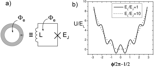
Figure 1.2: a) rf-SQUID and its equivalent circuit. b) Its potential energy as a function of phase for two different ratios of inductive $E_{L}$ and Josephson $E_{J}$ energies ($E_{L}=\Phi_{0}^{2}/2L$, $\Phi_{e}/\Phi_{0}=0.5$).

Depending on the ratio between charging and Josephson energies the dynamics of Josephson junctions can easily be analyzed in two respectfully extreme regimes. The limit $E_{C}\gg E_{J}$ is the one of the Cooper pair box and it was discussed earlier. In the opposite limit, $E_{J}\gg E_{c}$, the phase difference across the junction becomes a good quantum number that describes the quantized magnetic flux that is passing between the two electrodes of the junction. After the dropping of the constant $E_{J}$ term from (1.6), the Hamiltonian can be expressed in in the ”coordinate” representation $(n\rightarrow-i\partial_{\phi})$ as

$$H=E_{c}(i\partial_{\phi}+n_{q})^{2}-E_{J}\cos(\phi).$$ (1.7)

The periodic potential enables expressing the solutions of this Hamiltonian in the form of Bloch functions

$$|\Psi\rangle=u(\phi)e^{-in_{q}\phi},$$

where the continuous nature of $n_{q}$ gives rise to the existence of energy bands, while $u(\phi)$ has period of $2\pi$ and can be expressed in the terms of Mathew Functions [25].

The use of the Cooper pair dynamics for design of charge qubits was obvious after one junction electrode was made into a superconducting dot that trapped Cooper pairs. The Josephson flux dynamics can also be used for design of qubits by trapping the flux that passes through the junction on one of its sides as proposed in [26]. This requires inserting the junction into a superconducting ring as shown in figure 1.2a. The flux that passes through the junction from the right gets trapped inside the superconducting ring and in this process it induces a persistent current in the ring. This way shorted junction is called rf-SQUID.

Putting a junction into a superconducting loop of inductance $L$ gives rise to the inductive part in the Hamiltonian (1.7). The loop shorts the junction and the induced charge $n_{q}$ becomes irrelevant since it can always be screened out. Generally, some external flux $\Phi_{ext}$ can be applied to the loop and thus inductively coupled with the Josephson phase. Then the rf-SQUID Hamiltonian is

$$H=-E_{c}\partial_{\phi}^{2}-E_{J}\cos(\phi)+\frac{\Phi_{0}^{2}}{2L}(\phi/2\pi-\Phi_{ext}/\Phi_{0})^{2}.$$

The periodicity of (1.7) is clearly broken. Depending on the ratio of inductive energy $E_{L}=\Phi_{0}^{2}/2L$ and the Josephson tunneling $E_{J}$, the shape of the potential varies from one with a single minimum to one with many local potential minima (figure 1.2b). If $E_{L}/E_{J}\approx 3$ and $\Phi_{ext}/\Phi_{0}\approx 1/2$ the potential is characterized by two local minima (figure 1.3a) each corresponding to a different flux state that can mutually tunnel through the barrier, and whose relative energy spacing can be controlled by outside applied flux. This way optimized rf-SQUID can be used as qubit. The experiments [29, 30] have observed macroscopic quantum tunneling and the superposition of macroscopic persistent current states (figure 1.3b), but the need for the large inductance $L$ has hampered the observation of coherent oscillations since large inductance makes the qubit very sensitive to the fluctuations in the environment. As argued in [31], the need for the large inductance loop can be overcome by building a three-junction SQUID (figure 1.3c) characterized by smaller external inductance and thus less sensitive to the outside fluctuations. The ability of the three-junction SQUID to preform as a flux qubit was demonstrated in [32].

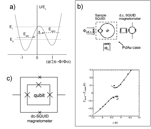
Figure 1.3: a) Energy levels for rf-SQUID for ${E_{L}/E_{C}=3}$, ${\Phi/\Phi_{o}=11/8\pi}$, $\Delta/E_{L}=0.06$. b) Experimental setup used in observing first superposition of quantum flux in a qubit and the plot of measured energy relative to the mean level energy as a function of bias $\varepsilon$. The plot clearly shows energy splitting caused by the existence of tunneling. For more see [30] c) Three-junction flux qubit and imbedded dc-SQUID magnetometer used for the first observation of flux qubit oscillations.

1.2.2 Long Junctions

If the junction interface is long, the passing of a fluxon between the electrodes cannot be considered instantaneous but rather as a real time event. In the certain limit of the junction parameters, the long junction supports the propagation of fluxons along the junction where the dynamics of the fluxons is affected by the injected or outside induced junction current. This way optimized long junction is often referred to as Josephson transmission line (JTL). At low temperatures these fluxons exhibits quantum dynamics [21], and they can be considered as individual quantum particles propagating in one or two-dimensional space, whose metric and the potential are fully determined by the junction parameters and the inserted current density respectively.

The varying phase of a long junction can be analyzed by treating the long junction as a distributed structure. In the case of a long junction with a varying superconducting phase along only one if its interfaces, the junction can be subdivided into strips with the strips treated as small junctions connected in parallel by inductors as shown in the lower part of figure 1.4. The Hamiltonian of this one-dimensional structure is given by

$$H=\sum_{n=1}^{N}\left\{\frac{q^{2}_{n}}{2C_{n}}-E_{Jn}\cos(\phi_{n})\right\}+\sum_{n=1}^{N-1}E_{Ln}\left(\phi_{n}-\phi_{n+1}\right)^{2},$$ (1.8)

where $q_{n}$ and $\phi_{n}$ are conjugate phase and charge variables of strip $n$ that satisfy $[\phi_{n},q_{m}]=2ei\delta_{n,m}$, while $C_{n}$, $E_{Jn}$ and $E_{Ln}$ are respectively the capacitance, Josephson tunneling, and inductive energy of the strips.

The equation (1.8) can be expressed in the continuous approximation if the limit where the strip size is much smaller than the length of the junction but larger than the superconducting penetration depth and the spacing between the electrodes. The continuous Lagrangian density of the uniform junction with length expressed in the units of Josephson penetration depth $\lambda_{J}$ and time in the units of plasma frequency $\omega_{p}$, reduces to the sine-Gordon Lagrangian

$${\cal{L}}_{SG} = \sqrt{\epsilon_{J}\epsilon_{L}}\left\{\frac{1}{2}(\partial_{\tau}\phi)^{2}-\frac{1}{2}(\partial_{x}\phi)^{2}+\cos(\phi)\right\}$$ (1.9)

$$\epsilon_{J}=\Phi_{0}J_{c}/2\pi, \epsilon_{L}=(\Phi_{0}/2\pi)^{2}/l_{0},\qquad\omega_{p}^{2}=\epsilon_{j}/c_{0},\qquad\lambda_{J}^{2}=\epsilon_{L}/\epsilon_{J},$$

where $J_{c}$, $c_{0}$ and $l_{0}$ are Josephson current density, junction capacitance density and inductance density respectively.

In the framework of semi-classical quantization of sine-Gordon Lagrangian [33], the propagating fluxon is represented as a relativistic soliton of size $\pi\lambda_{J}$. The average position and velocity of the soliton are specified by its two collective coordinates, while the other coordinates correspond to the internal quantum excitations of the soliton. At low temperatures ($k_{B}T\ll\sqrt{\epsilon_{J}\epsilon_{L}}$), and as long as the velocity of fluxon is not on the order of $\lambda_{J}\omega_{p}$, the fluxon cannot excite these internal degrees of freedom. It behaves as a relativistic quantum particle of mass $M=\sqrt{2\epsilon_{J}\epsilon_{L}}/\lambda_{J}^{2}\omega_{p}^{2}$ propagating free in one-dimensional relativistic space with ”speed of light” given as $c=\lambda_{J}\omega_{p}$.

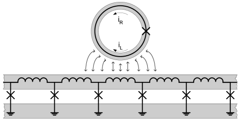
Figure 1.4: Long Josephson junction, depicted in the bottom of the drawing, can be viewed as distributed structure consisting of small Josephson junctions connected in parallel by inductors. In the certain limit of the junction parameters, the long junction supports propagation of fluxons in between its interfaces. It can perform as a detector, since the near-by flux qubit couples to it inductively and modulates the scattering matrix of the propagating fluxons.

Coupling a flux qubit with the JTL (figure 1.4) creates potential in the JTL, and the Hamiltonian (1.8) and Lagrangian (1.9) get a source term whose explicit form depends on the type and strength of coupling. In any case, the source term is localized as long as the qubit size is much smaller than the JTL, and the freely propagating fluxons will now scatter off the potential caused by the localized source term and the transmission properties of the 1-D channel formed by the optimized JTL will depend on the qubit state. This setup can be used for determining the state of the qubit, but if not designed properly the propagating fluxons along the JTL will interact with the qubit and cause decoherence.

1.3 Modelling Decoherence

The qubits introduced above are affected by the changes in the environment. This is not just caused by the measurement of the qubit, rather it can be contributed to many other factors. For example, 1/f charge fluctuations induce variations of the static Coopers in the pair box, while the inductive loop of the rf-SQUID easily couples the flux qubit with the outside electromagnetic fluctuations that vary the bias of the qubit. The coupling of the qubit with the outside noise sources adds additional degrees of freedom to the system whose random nature smear the coherent phase of the condensates and decohere the qubit. In many cases the microscopic origin of the decoherence is unknown. Therefore, to study the decoherence it is necessary to devise a model that treats the qubit as a quantum system in contact with some general environment which in the appropriate limit reduces to a stochastic process.

System-plus-bath or system-plus-reservoir is the most natural way to approach this problem. It considerers the weak entanglement between the system of interest $S$, and the much larger surroundings that act as a heat bath or a reservoir [34, 35, 36]. Reducing the general equations of motion by tracing-out the environmental degrees of freedom leaves the equations dependent explicitly only on $S$. In this process the environment is assumed classical, static, and unaffected by $S$. Thus any energy that moves from $S$ is not stored, but lost in the environment. This results in slow, irreversible transfer of the energy from $S$ to the environment that is reflected in the reduced equations of motion. In the further works [37, 38, 39], the general reservoir was replaced by infinite number of harmonic oscillators. This took into an account that the environment by itself is a quantum system and relaxed the earlier condition of strictly classical environment.

Spin-Boson is the common name for the model that precipitates after the system-plus-reservoir model is applied to a quantum two-level system [40]. Explicitly, it consists of the qubit Hamiltonian (1.2) linearly coupled to a bath consisted of a large number of harmonic oscillators

$$H_{SB}=H+\frac{\hbar}{2}\sigma_{z}\sum_{i=1}^{N}\lambda_{i}(c_{i}+c^{{\dagger}}_{i})+\sum_{i=1}^{N}\hbar\omega_{i}c^{{\dagger}}_{i}c_{i},$$ (1.10)

where $c_{i}$ and $c^{{\dagger}}_{i}$ are creation and annihilation operators, and $\lambda_{i}$ is the coupling between the $i$-th oscillator and the qubit. The environmental effects are phenomenologically represented by the noise spectral density $S(\omega)$ of the coupling

$$S(\omega)=\sum_{i=1}^{N}\lambda_{i}^{2}\delta(\omega-\omega_{i}).$$ (1.11)

For weak coupling, the qubit will slowly couple to the oscillators in the bath, and in the large oscillator bath limit $(N\rightarrow\infty)$, the energy dissipated by the qubit will never come back. As a consequence, the qubit will relax to some energy equilibrium state determined by the qubit-bath coupling. This equilibrium state will effectively become the ground state of the qubit and for this reason the qubit will become static and stop exhibiting coherent oscillations.

1.4 Quantum Measurement

In order to measure the qubit it is necessary to entangle it with a detector whose classical output signal is correlated with the state of the qubit. Because of the entanglement, a definite state of the output signal localizes the qubit in one of the states determined by the detector-qubit coupling. This is the same process as the reservoir induced decoherence discussed earlier. The major difference is that the extracted information from the qubit is not all lost, but that a part or preferably all of it is reflected in the detector output.

Single-shot measurement is characterized by perfect correlation between the qubit and the detector output. This requires strong coupling between the detector and the qubit. Thus measuring the qubit extracts all the information and instantaneously collapses the qubit into the state correlated with the observed output.

As an example we can consider the setup as shown in figure 1.4, where the JTL is situated close to the flux qubit consisting of appropriately optimized rf-SQUID. In the case of negligible decoherence and strong inductive coupling between the qubit and JTL, a fluxon propagating from the left along the transmission line is totally reflected if the qubit is in $|R\rangle$ state, and totally transmitted if the qubit is in the $|L\rangle$ state. So after the scattering, the transmitted fluxon is entangled with the $|L\rangle$ and vice-versa. Detecting weather the fluxon was reflected of transmitted will collapse the qubit into the state entangled with the scattering outcome.

In order to recover the statistical properties of the superposition state of the qubit, it is necessary to repeat the single-shot measurement on a certain number of the identically prepared and time evolved qubits [41]. The observation of the quantum coherent oscillations of the qubit requires further measurement of the superpositions at different times.

Coupling the qubit weakly with the detector does not result in instantaneous wave function collapse, and for this reason the measurement provides only limited information about the qubit. This is reflected in the detector output which is not perfectly correlated with the qubit, rather it is characterized by existence of the overlap between the two signals that represent the corresponding qubit states.

If the qubit and JTL in the earlier example are weakly coupled, the fluxon scattering matrix is only affected partially by the state of the qubit. The transmitted or reflected fluxon is entangled with both states of the qubit. Detecting the scattering outcome in this case does not collapse the qubit, but provides information in which state the qubit is more likely to be.

The advantage of the weakly coupled detector is its ability to monitor qubit continuously for some time. During the measurement process, the qubit will slowly localize under the influence of the detector back-action which does not necessarily keep the qubit coherent, rather the off-diagonal density matrix element in the flux basis is limited from above as $|\sigma_{LR}(t)|\leq\sqrt{\sigma_{LL}(t)\sigma_{RR}(t)}$.

The back-action dephasing and the continuous extraction of information are two parallel dynamical processes where the rate of back-action induced dephasing is never smaller that the rate of information extraction. In the ideal case of the two rates being equal, the detector back-action keeps the qubit coherent, and the detector will extract information form the qubit as fast as it is localizing it. Any deviation from the ideal measurement will result in loss of information since the decoherence rate will be larger than the information extraction rate. This is a general result that can be obtained from linear response theory [42] applied to a Hamiltonian $H=H_{q}+H_{d}+xf$, where $H_{q}$ and $H_{d}$ are general quantum system and detector respectively that are linearly connected through a general quantum system coordinate $x$ and some detector ”force” $f$. The detector provides output signal $o(t)$ that consists of the detector nose $q(t)$ and response $\lambda x(t)$.

Assuming that the detector is static, the dynamics of the measurement is determined by three correlators of detector parameters that describe detector back-action $\langle f(0)f(t)\rangle$, detector response $\langle f(0)q(t)\rangle$, and the output nose $\langle q(0)q(t)\rangle$. In this framework, the condition of the ideal measurement is generalized of having detector satisfy $Re(\langle q(0)f(t)\rangle)=0$. Furthermore, it can be shown that in the case of the ideal measurement of coherent oscillations the detector signal-to-noise ratio is limited to four from above [43].

This limitation is a direct consequence of the detector back-action and it can be traced back to the nature of the detector-qubit coupling. If $x$ in the coupling is to be made a constant of motion of the measured system, then the detector would preform quantum non-demolition (QND) measurement that has no upper limit on the signal to noise ratio [44]. To illustrate QND measurement consider fluxons propagating along the JTL detector weakly coupled to the flux qubit. If the fluxon insertion frequency equals to the qubit frequency, the passing fluxons will ”kick” the qubit in exactly the same way and in this process exert no back-action on the qubit. This detector will thus be able to determine the flux state of the qubit, but it will also make the qubit static in the basis of detector coupling [45].

Part I Quantum Decoherence

Chapter 2 Weakly Coupled High-Frequency Noise

The purpose of this chapter is to develop theoretical description of decoherence in the case of two coupled qubits subject to high frequency (high-f) noise. It follows a standard, Markovian approximation approach for description of weak decoherence based on the perturbation expansion of the density matrix evolution equation. The result obtained within this simple scheme is useful as a starting point for noise treatment of coupled qubit systems and as a benchmark for more elaborate models.

2.1 The Model

The model is a system-plus-bath model where an arbitrary number of quantum operators $Q_{i}$ of the quantum system $H_{0}$ are each weakly connected with a different bath $H_{B}^{(i)}$ though a generalized bath force $f_{i}$. The baths can be correlated. Furthermore, they are assumed to be much larger that the quantum system and initially in an equilibrium. The large size and the weak coupling makes the baths unaffected by the qubit. They remain in equilibrium and can be separated out from the total density matrix of the system. Explicitly, $\rho_{tot}(t)=\rho(t)\rho_{B}$, where the two density matrices on the right respectively describe the tensor product of quantum system and the total ”bath-described” environment.

If the system is initialized at $t=0$, its Hamiltonian

$$H=H_{0}+\sum_{i}H_{B}^{(i)}+\sum_{i}f_{i}Q_{i},$$ (2.1)

expanded to the second order in the coupling yields differential equation that describes the evolution of the qubit’s density matrix in the interaction picture as:

$$\dot{\rho}(t) = -\frac{i}{\hbar}\sum_{i}tr_{B}\{\left[f_{i}(t)Q_{i}(t),\rho(0)\rho_{B}\right]\}$$

$$- \frac{1}{\hbar^{2}}\sum_{ij}\int_{0}^{t}dt^{\prime}tr_{B}\{\left[f_{i}(t)Q_{i}(t),\left[f_{j}(t^{\prime})Q_{j}(t^{\prime}),\rho(t^{\prime})\rho_{B}\right]\right]\}.$$

In the equation (2.1), the force operators can be factored out and grouped into their expectation values $\langle f_{i}(t)\rangle$ and correlations $\langle f_{i}(t)f_{j}(t^{\prime})\rangle$, where $\langle\cdots\rangle\equiv tr_{B}\{\rho_{B}\cdots\}$. Since $H_{0}$ can always be renormalized to absorb the non-diagonal force operators ($\langle f_{i}(t)\rangle\neq 0$), it can be assumed that $\langle f_{i}(t)\rangle\equiv 0$ and that the environment is represented only by the force correlators. According to the central limit theorem (eg. see [46]) and the the Wick theorem [47, 40] using the second order correlators to describe the noise created by a large system is sufficient. The central limit theorem implies that the macroscopic size of the environment makes the noise generated by it Gaussian, while the higher order correlators of Gaussian noise are always expressible by Wick’s theorem in the terms of second order correlators. Therefore, the correlators $\langle f_{i}(t)f_{j}(t^{\prime})\rangle$ or equivalently their spectral densities

$$S_{ij}(\omega)=\int_{-\infty}^{\infty}\langle f_{i}(0)f_{j}(t)\rangle e^{i\omega t}dt,$$ (2.3)

fully describe the environment in our case.

The further assumption of Markovian nature of the system, implies that $\dot{\rho}(t)$ depends only on $\rho(t)$ and justifies replacing $\rho(t^{\prime})\rightarrow\rho(t)$ in the integral part of the equation (2.1). The high frequency nature of the noise makes the bath response time instantaneous and the integration limit in (2.1) can be extended to infinity. The differential equation (2.1) simplifies to

$$\dot{\rho}(t)=-\frac{1}{\hbar^{2}}\sum_{ij}\int_{0}^{\infty}dt^{\prime}\left\{\left[Q_{i}(t),Q_{j}(t-t^{\prime})\rho(t)\right]\langle f_{i}(t^{\prime})f_{j}(0)\rangle\right.$$

$$-\left.\left[Q_{i}(t),\rho(t)Q_{j}(t-t^{\prime})\right]\langle f_{j}(0)f_{i}(t^{\prime})\rangle\right\}.$$ (2.4)

Expressing the operators $Q_{i}(t)$ in the interaction representation, (i.e. $Q_{i}(t)=\exp(it\hat{H}_{0}/\hbar)Q_{i}(0)\exp(-it\hat{H}_{0}/\hbar)$) and then recognizing that all but non-oscillatory terms of the equation (2.1) average out, yields differential matrix equation that describes the relaxation of the quantum system. The equation is in general solvable but progressively more complicated with the increasing energy spectrum of $H_{0}$.

2.2 Single Qubit

Long and extensive history of studying two-level quantum systems in optics and NMR calls for the discussion about the decoherence in a single qubit to be very short. The more detailed derivation of the results can be found in standard literature, i.e. [48].

We start by specifying the two-level system coupled to a bath through its vertical polarization

$$H=-\frac{\hbar}{2}\left[\varepsilon\sigma_{z}+\Delta\sigma_{x}\right]-\frac{\hbar f}{2}\sigma_{z}+H_{B},$$

with the bias $\varepsilon$, tunnelling $\Delta$ and noise $f$ all having units of frequency. The choice of the coupling corresponds to the electrostatic interaction through finite coupling capacitance for charge qubits, or magnetic interaction for flux qubits. The interaction part of the Hamiltonian in the interaction basis is:

$$H_{int}^{diag}=-\frac{\hbar f}{2\sqrt{\varepsilon^{2}+\Delta^{2}}}\left[\varepsilon\sigma_{z}-\Delta\sigma_{x}\right].$$

After following all the steps outlined above, it is easy to arrive to standard two-level relaxation result that implies longest coherence times and shortest relaxation times for qubits operating at zero-bias, ($\epsilon=0$), point. The relaxation rate at this optimal point is $\Gamma\equiv 1/T_{1}=S(\Delta)/2$ while the decoherence rate is $\gamma\equiv 1/T_{2}=S(\Delta)/4$. Consistent to Fermi’s golden rule they are different by factor-of-2.

2.3 Double Qubit

Motivation for studying decoherence in coupled qubits is provided by the first successful double charge qubit experiment [20], where it was found that the decoherence rate for quantum coherent oscillations in two qubits at the optimal bias point is with good accuracy factor-of-four larger than the decoherence rate in effectively decoupled qubits. An interesting question for theory is whether this factor-of-four increase of the decoherence rate is a numerical coincidence, or it reflects some basic property of the decoherence mechanisms in charge qubits. As will become clear from the discussion below, the theory developed in this section favors “numerical coincidence” point of view. Other aspects of decoherence in coupled qubits have been studied before numerically in [49, 50, 51].

In general, it is well understood that decoherence rates of different states of two coupled qubits can be quite different if the random forces created by the qubit environments responsible for decoherence are completely or partially correlated. Most importantly, in the case of complete correlation, the qubit system should have a “decoherence-free subspace” (DFS) spanned by the states $|01\rangle$, $|10\rangle$ [48, 12, 49], since completely correlated external environments can not distinguish these states. In contrast, the subspace spanned by $|00\rangle$ and $|11\rangle$ experiences decoherence that is made stronger by the correlations between environmental forces acting on the two qubits. So the role of the quantitative theory in description of decoherence in the dynamics of coupled qubits is to see to what extent subspaces with different decoherence rates participate in the qubit oscillations for different methods of their excitation.

2.3.1 The model and environmental correlations

The Hamiltonian of the system of two qubits coupled directly by interaction between the basis-forming degrees of freedom is:

$$H_{0}=\hbar\sum_{j=1,2}(\varepsilon_{j}\sigma_{z}^{(j)}+\Delta_{j}\sigma_{+}^{(j)}+\Delta_{j}^{*}\sigma_{-}^{(j)})+\hbar\nu\sigma_{z}^{(1)}\sigma_{z}^{(2)}\,,$$ (2.5)

where $\sigma$’s denote the Pauli matrices, $\nu$ is the qubit interaction energy, $\Delta_{j}$ is the tunnel amplitude and $\varepsilon_{j}$ is the bias of the $j$-th qubit. Four energy levels of the Hamiltonian (2.5) are shown schematically in figure 2.1 as functions of the common bias $\bar{\varepsilon}\equiv\varepsilon_{1}=\varepsilon_{2}$ of the two qubits. This work considers quantum coherent oscillations in the qubits biased at the “co-resonance” point [20], where $\varepsilon_{1}=\varepsilon_{2}=0$. Such bias conditions are optimal for the oscillations.

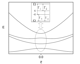
Figure 2.1: Schematic structure of the energy levels of the two coupled qubits as functions of the common bias of the qubits. The inset shows the diagram of the decoherence-induced transitions between the levels at “co-resonance” point where the bias vanishes.

It can be shown explicitly that the occupation probabilities of the qubit basis states (that are of interest for us) are insensitive to the phases of the qubit tunnel amplitudes $\Delta_{j}$, so without the loss of generality we will assume that $\Delta_{j}$’s are real. The Hamiltonian (2.5) at the co-resonance reduces then to

$$H_{0}=\hbar\sum_{j=1,2}\Delta_{j}\sigma_{x}^{(j)}+\hbar\nu\sigma_{z}^{(1)}\sigma_{z}^{(2)}\,.$$ (2.6)

In the basis composed of eigenstates of the $\sigma_{x}^{(j)}$ operators, the Hamiltonian (2.6) can be diagonalized easily. Eigenenergies and eigenstates are:

$$E_{1}=\hbar\Omega, |\psi_{1}\rangle=\frac{1}{2}[(\gamma+\eta)(|00\rangle+|11\rangle)+(\eta-\gamma)(|01\rangle+|10\rangle)],$$

$$E_{2}=-\hbar\Omega, |\psi_{2}\rangle=\frac{1}{2}[(\gamma-\eta)(|00\rangle+|11\rangle)+(\gamma+\eta)(|01\rangle+|10\rangle)],$$ (2.7)

$$E_{3}=\hbar\epsilon, |\psi_{3}\rangle=\frac{1}{2}[(\alpha+\beta)(|00\rangle-|11\rangle)+(\alpha-\beta)(|10\rangle-|01\rangle)],$$

$$E_{4}=-\hbar\epsilon, |\psi_{4}\rangle=\frac{1}{2}[(\beta-\alpha)(|00\rangle-|11\rangle)+(\alpha+\beta)(|10\rangle-|01\rangle)],$$

where

$$\Omega=(\Delta^{2}+\nu^{2})^{1/2},\qquad\epsilon=(\delta^{2}+\nu^{2})^{1/2},\qquad$$

$$\alpha,\beta=\frac{1}{\sqrt{2}}\left(1\pm\frac{\delta}{\epsilon}\right)^{1/2}\,,\;\;\;\eta,\gamma=\frac{1}{\sqrt{2}}\left(1\pm\frac{\Delta}{\Omega}\right)^{1/2}$$

and $\Delta\equiv\Delta_{1}+\Delta_{2}$, $\delta\equiv\Delta_{1}-\Delta_{2}$. The states $|kl\rangle$ with $\{k,l\}=\{0,1\}$ in equations (2.7) are the eigenstates of the operators $\sigma_{z}^{(1,2)}$ in the natural notations: $\sigma_{z}^{(1)}|kl\rangle=(-1)^{k}|kl\rangle$ and $\sigma_{z}^{(2)}|kl\rangle=(-1)^{l}|kl\rangle$.

We assume that external environments responsible for the decoherence couple to the basis-forming degrees of freedom of the qubits. The interaction Hamiltonian is then:

$$H_{i}=\hbar\sum_{j=1,2}f_{j}(t)\sigma_{z}^{(j)}\,.$$ (2.8)

The random forces $f_{1,2}(t)$ acting on the qubits are in general correlated. To describe the weakly dissipative dynamics of the system in the basis of states (2.7) induced by the interaction (2.8) with the reservoirs, we use the standard equation (2.1). Proceeding in the usual way, we keep in equation (2.1) only the terms that do not oscillate, and therefore lead to changes in $\rho$ that accumulate over time. Equations for the matrix elements $\rho_{nm}$, $n,m=1,...,4$, of $\rho$ in the basis (2.7) are transformed then as follows:

$$\dot{\rho}_{nm} = \sum_{j,j^{\prime}=1,2}\big{[}-\rho_{nm}(\sigma_{mm}^{(j)}-\sigma_{nn}^{(j)})(\tilde{S}_{jj^{\prime}}^{*}(0)\sigma_{mm}^{(j^{\prime})}-\tilde{S}_{jj^{\prime}}(0)\sigma_{nn}^{(j^{\prime})})$$ (2.9)

$$-\rho_{nm}\sum_{k}(\sigma_{nk}^{(j)}\sigma_{kn}^{(j^{\prime})}\tilde{S}_{jj^{\prime}}(\epsilon_{n}-\epsilon_{k})+\sigma_{mk}^{(j^{\prime})}\sigma_{km}^{(j)}\tilde{S}_{jj^{\prime}}^{*}(\epsilon_{m}-\epsilon_{k}))$$

$$+\delta_{nm}\sum_{k}\rho_{kk}(\sigma_{nk}^{(j^{\prime})}\sigma_{kn}^{(j)}\tilde{S}_{jj^{\prime}}(\epsilon_{k}-\epsilon_{n})+\sigma_{nk}^{(j)}\sigma_{kn}^{(j^{\prime})}\tilde{S}_{jj^{\prime}}^{*}(\epsilon_{k}-\epsilon_{n})$$

$$+\sum_{(k,l)}\rho_{kl}\sigma_{nk}^{(j^{\prime})}\sigma_{lm}^{(j)}(\tilde{S}_{jj^{\prime}}(\epsilon_{l}-\epsilon_{m})+\tilde{S}_{j^{\prime}j}^{*}(\epsilon_{l}-\epsilon_{m}))\big{]}.$$

Here $\sigma_{nm}^{(j)}$ denote the matrix elements $\langle n|\sigma_{z}^{(j)}|m\rangle$, the last sum is taken over the pairs $(k,l)$ of states that satisfy the “resonance” condition:

$$\epsilon_{k}-\epsilon_{l}=\epsilon_{n}-\epsilon_{m}\,,\;\;\;(k,l)\neq(n,m)\,,$$

and

$$\tilde{S}_{jj^{\prime}}(\omega)=\int_{0}^{\infty}dt\langle f_{j}(t)f_{j^{\prime}}(0)\rangle e^{i\omega t}\,.$$

The first term in equation (2.9) represents “pure dephasing” that exists when the system operators that couple it to the environment have non-vanishing average values in the eigenbasis. As one can see explicitly from equations (2.7), the average values $\sigma_{nn}^{(j)}$ of $\sigma_{z}^{(j)}$ are vanishing in all states, so that there is no pure dephasing term in the evolution of the density matrix in our case. The fact that $\sigma_{nn}^{(j)}$ are vanishing can be related to the vanishing slope of the system energies with respect to variations of the bias in the vicinity of the co-resonance point – see figure 2.1. Since all coefficients in the eigenfunctions (2.7) are real, the matrix elements $\sigma_{nm}^{(j)}$ are also real. For real $\sigma_{nm}^{(j)}$, imaginary parts of the noise correlators $\tilde{S}_{j^{\prime}j}$ in the second term on the right-hand-side of equation (2.9) represent the decoherence-induced shifts of the systems’ energy levels. These shifts do not affect decoherence and we will neglect them in our discussion. With these simplifications, equation (2.9) takes the form

$$\dot{\rho}_{nm}=$$ (2.10)

$$\sum_{j,j^{\prime}=1,2}\big{[}-(\rho_{nm}/2)\sum_{k}(\sigma_{nk}^{(j)}\sigma_{kn}^{(j^{\prime})}\mbox{Re}S_{jj^{\prime}}(\epsilon_{n}-\epsilon_{k})+\sigma_{mk}^{(j^{\prime})}\sigma_{km}^{(j)}\mbox{Re}S_{jj^{\prime}}(\epsilon_{m}-\epsilon_{k}))$$

$$+\delta_{nm}\sum_{k}\rho_{kk}\sigma_{nk}^{(j^{\prime})}\sigma_{kn}^{(j)}\mbox{Re}S_{jj^{\prime}}(\epsilon_{k}-\epsilon_{n})+\sum_{(k,l)}\rho_{kl}\sigma_{nk}^{(j^{\prime})}\sigma_{lm}^{(j)}S_{jj^{\prime}}(\epsilon_{l}-\epsilon_{m})\big{]},$$

where

$$S_{jj^{\prime}}(\omega)=\int_{-\infty}^{\infty}dt\langle f_{j}(t)f_{j^{\prime}}(0)\rangle e^{i\omega t}\,.$$ (2.11)

The function $S_{12}$ characterizes the correlations between the environmental forces acting on the two qubits. For instance, if the two qubits interact with different environments and $v_{1}$, $v_{2}$ are uncorrelated, $S_{12}=0$, whereas $S_{12}=S_{11}=S_{22}$, if the qubits are acted upon by the force produced by a single environment coupled equally to the two qubits. While the correlators $S_{11}$ and $S_{22}$ are strictly real, $S_{12}$ can be imaginary, and $S_{21}^{*}=S_{12}$. Non-vanishing imaginary part of $S_{12}$ corresponds to the non-vanishing commutator $[f_{1},f_{2}]$ and implies that the two qubits are coupled to the two non-commuting variables of the same reservoir. While this is probably not very likely for qubits with the basis-forming degrees of freedom of the same nature (which in a typical situation should be coupled to the same set of environmental degrees of freedom), the non-vanishing $\mbox{Im}S_{12}$ should be typical if the qubits have different basis-forming variables,(e.g. see system proposed in [52]). Using the spectral decomposition of the correlators $S_{jj^{\prime}}(\omega)$ and Schwartz inequality, one can prove that for arbitrary stationary reservoirs the correlators satisfy the inequality that imposes the constraint on $S_{12}(\omega)$:

$$S_{11}(\omega)S_{22}(\omega)\geq|S_{12}(\omega)|^{2}\,.$$ (2.12)

If the reservoirs are in equilibrium at temperature $T$, the correlators also satisfy the standard detailed balance relations:

$$S_{jj^{\prime}}(-\omega)=e^{-\frac{\hbar\omega}{k_{B}T}}S_{j^{\prime}j}(\omega)\,.$$ (2.13)

Equation (2.10) with the noise correlators (2.11) govern weakly dissipative time evolution of the two coupled qubits in a generic situation. Below we use them to determine decoherence properties of quantum coherent oscillations of the qubits.

2.3.2 Quantum coherent oscillations in coupled qubits

One of the most direct ways of excitation of quantum coherent oscillations in individual or coupled qubits that will be discussed in this work is based on the abrupt variation of the bias conditions [18, 20]. If the qubits are initially localized in one of their basis states, e.g. $|00\rangle$, and abrupt variation of the bias brings them to the co-resonance point, the probabilities for the qubits to be in other basis states start oscillating with time.

In the simplest detection scheme (realized, for instance, in experiment [20]) the probability for each qubit to be in the state $|1\rangle$ is measured independently of the state of the other qubit. Quantitatively, these probabilities $p_{j}$ are obtained from the projection operators $P_{j}$:

$$p_{j}=\mbox{Tr}\{\rho P_{j}\}\,,\;\;\;P_{1}=\sum_{k=1,2}|1k\rangle\langle k1|\,,\;\;\;P_{2}=\sum_{k=1,2}|k1\rangle\langle 1k|\,.$$ (2.14)

Finding explicitly the matrix elements of $P_{j}$ from the wave functions (2.7), one gets:

$$p_{1}(t)=\frac{1}{2} + (\alpha\eta+\beta\gamma)\mbox{Re}[e^{-i\omega_{-}t}(\rho_{42}(t)-\rho_{13}(t))]$$ (2.15)

$$+ (\alpha\gamma-\beta\eta)\mbox{Re}[e^{-i\omega_{+}t}(\rho_{14}(t)+\rho_{32}(t))]\,,$$

$$p_{2}(t)=\frac{1}{2} - (\alpha\gamma+\beta\eta)\mbox{Re}[e^{-i\omega_{-}t}(\rho_{13}(t)+\rho_{42}(t))]$$ (2.16)

$$+ (\alpha\eta-\beta\gamma)\mbox{Re}[e^{-i\omega_{+}t}(\rho_{14}(t)-\rho_{32}(t))]\,,$$

where $\omega_{\pm}\equiv\Omega\pm\epsilon$, and as in the equation (2.10), the matrix elements of the density matrix are taken in the interaction representation. Equations (2.15), (2.16), and (2.9) show that the waveform of the coherent oscillations in coupled qubits is determined by the time evolution of the two pairs of the matrix elements of $\rho$:

$$\dot{\rho}_{13}=-\Gamma_{13}\rho_{13}+u_{-}\rho_{42}\,,\;\;\;\dot{\rho}_{42}=-\Gamma_{42}\rho_{42}+u_{+}\rho_{13}\,,$$ (2.17)

$$\dot{\rho}_{14}=-\Gamma_{14}\rho_{14}+v_{-}\rho_{32}\,,\;\;\;\dot{\rho}_{32}=-\Gamma_{32}\rho_{32}+v_{+}\rho_{14}\,.$$ (2.18)

The decoherence rates in these equations are determined by the rates of transitions between different energy eigenstates:

$$\Gamma_{13}=\frac{1}{2}\big{(}\Gamma_{1}^{(+)}+\Gamma_{2}^{(-)}+\Gamma_{2}^{(+)}+\Gamma_{4}^{(+)}\big{)},$$

$$\Gamma_{14}=\frac{1}{2}\big{(}\Gamma_{1}^{(-)}+\Gamma_{1}^{(+)}+\Gamma_{2}^{(+)}+\Gamma_{3}^{(+)}\big{)},$$

$$\Gamma_{32}=\frac{1}{2}\big{(}\Gamma_{2}^{(-)}+\Gamma_{3}^{(-)}+\Gamma_{4}^{(-)}+\Gamma_{4}^{(+)}\big{)},$$

$$\Gamma_{42}=\frac{1}{2}\big{(}\Gamma_{1}^{(-)}+\Gamma_{3}^{(-)}+\Gamma_{3}^{(+)}+\Gamma_{4}^{(-)}\big{)}\,.$$ (2.19)

where labelling of the transitions is indicated in the inset in figure 2.1. Transition rates are:

$$\Gamma_{1}^{(\pm)}=\mbox{Re}\sum_{j,j^{\prime}}S_{jj^{\prime}}(\pm\omega_{+})\sigma_{14}^{(j)}\sigma_{41}^{(j^{\prime})}\,,$$

$$\Gamma_{2}^{(\pm)}=\mbox{Re}\sum_{j,j^{\prime}}S_{jj^{\prime}}(\pm\omega_{-})\sigma_{13}^{(j)}\sigma_{31}^{(j^{\prime})}\,,$$

$$\Gamma_{3}^{(\pm)}=\mbox{Re}\sum_{j,j^{\prime}}S_{jj^{\prime}}(\pm\omega_{-})\sigma_{24}^{(j)}\sigma_{42}^{(j^{\prime})}\,,$$

$$\Gamma_{4}^{(\pm)}=\mbox{Re}\sum_{j,j^{\prime}}S_{jj^{\prime}}(\pm\omega_{+})\sigma_{23}^{(j)}\sigma_{32}^{(j^{\prime})}\,.$$ (2.20)

The superscripts $\pm$ refer here to transitions in the direction of decreasing (+) or increasing (-) energy. After finding matrix elements $\sigma_{nm}$ from the wave functions (2.7), we see explicitly that transitions between the states 1 and 2, as well as 3 and 4 are suppressed. Since the corresponding matrix elements are zero, the rates (2.20) are:

$$\Gamma_{1} = \frac{1}{2}S_{11}\left[1-\frac{\delta\Delta+\nu^{2}}{\epsilon\Omega}\right]+\frac{1}{2}S_{22}\left[1+\frac{\delta\Delta-\nu^{2}}{\epsilon\Omega}\right]-\mbox{Re}S_{12}\frac{\nu\omega_{-}}{\Omega\epsilon}\,,$$

$$\Gamma_{2} = \frac{1}{2}S_{11}\left[1+\frac{\delta\Delta+\nu^{2}}{\epsilon\Omega}\right]+\frac{1}{2}S_{22}\left[1-\frac{\delta\Delta-\nu^{2}}{\epsilon\Omega}\right]+\mbox{Re}S_{12}\frac{\nu\omega_{+}}{\Omega\epsilon}\,,$$

$$\Gamma_{3} = \frac{1}{2}S_{11}\left[1+\frac{\delta\Delta+\nu^{2}}{\epsilon\Omega}\right]+\frac{1}{2}S_{22}\left[1-\frac{\delta\Delta-\nu^{2}}{\epsilon\Omega}\right]-\mbox{Re}S_{12}\frac{\nu\omega_{+}}{\Omega\epsilon}\,,$$ (2.21)

$$\Gamma_{4} = \frac{1}{2}S_{11}\left[1-\frac{\delta\Delta+\nu^{2}}{\epsilon\Omega}\right]+\frac{1}{2}S_{22}\left[1+\frac{\delta\Delta-\nu^{2}}{\epsilon\Omega}\right]+\mbox{Re}S_{12}\frac{\nu\omega_{-}}{\Omega\epsilon}\,.$$

The transfer “rates” $u$, $v$ in equations (2.17) and (2.18) are:

$$u_{\pm}=\sum_{j,j^{\prime}=1,2}\sigma_{14}^{(j^{\prime})}\sigma_{32}^{(j)}S_{jj^{\prime}}(\pm\omega_{+})\,,\;\;\;v_{\pm}=\sum_{j,j^{\prime}=1,2}\sigma_{13}^{(j^{\prime})}\sigma_{42}^{(j)}S_{jj^{\prime}}(\pm\omega_{-})\,.$$ (2.22)

Explicitly:

$$u=\frac{1}{2}S_{11}\left[1-\frac{\delta\Delta+\nu^{2}}{\epsilon\Omega}\right]-\frac{1}{2}S_{22}\left[1+\frac{\delta\Delta-\nu^{2}}{\epsilon\Omega}\right]-i\mbox{Im}S_{12}\frac{\nu\omega_{-}}{\Omega\epsilon}\,,$$

$$v=-\frac{1}{2}S_{11}\left[1+\frac{\delta\Delta+\nu^{2}}{\epsilon\Omega}\right]+\frac{1}{2}S_{22}\left[1-\frac{\delta\Delta-\nu^{2}}{\epsilon\Omega}\right]-i\mbox{Im}S_{12}\frac{\nu\omega_{+}}{\Omega\epsilon}\,.$$ (2.23)

Equations (2.21) and (2.23) do not show the frequency dependence of noise correlators, which is the same, respectively, as in the equations (2.20) and (2.22).

Each pair, (2.17) and (2.18), of coupled equations can be solved directly by diagonalization of the matrix of the evolution coefficients with a non-orthogonal transformation. In this way we obtain for the pair of equations (2.17):

$$\rho_{13}(t)=\frac{\big{[}\rho_{13}(0)(u_{+}u_{-}e^{-\gamma_{+}t}+c^{2}e^{-\gamma_{-}t})+cu_{-}\rho_{42}(0)(e^{-\gamma_{+}t}-e^{-\gamma_{-}t})\big{]}}{u_{+}u_{-}+c^{2}}\,,$$

$$\rho_{42}(t)=\frac{\big{[}\rho_{42}(0)(u_{+}u_{-}e^{-\gamma_{-}t}+c^{2}e^{-\gamma_{+}t})+cu_{+}\rho_{13}(0)(e^{-\gamma_{+}t}-e^{-\gamma_{-}t})\big{]}}{u_{+}u_{-}+c^{2}}\,.$$ (2.24)

where

$$\gamma_{\pm}\equiv(\Gamma_{13}+\Gamma_{42})/2\pm\big{[}(\Gamma_{13}-\Gamma_{42})^{2}/4+u_{+}u_{-}\big{]}^{1/2}\,,$$

$$c\equiv(\Gamma_{13}-\Gamma_{42})/2-\big{[}(\Gamma_{13}-\Gamma_{42})^{2}/4+u_{+}u_{-}\big{]}^{1/2}\,,$$ (2.25)

and $\rho_{13}(0)$, $\rho_{42}(0)$ are the initial values of the density matrix elements that depend on preparation of the initial state. If, as in the experiment [20], the qubits are abruptly driven to co-resonance maintaining the state $|00\rangle$, these initial values are:

$$\rho_{13}(0) = \frac{1}{4}(\gamma+\eta)(\alpha+\beta)\,,\;\;\;\rho_{32}(0)=\frac{1}{4}(\gamma-\eta)(\alpha+\beta)\,,$$

$$\rho_{14}(0) = \frac{1}{4}(\gamma+\eta)(\beta-\alpha)\,,\;\;\;\rho_{42}(0)=\frac{1}{4}(\gamma-\eta)(\alpha-\beta)\,.$$ (2.26)

Another type of initial conditions that will be discussed in this work is starting the oscillations from the state $|10\rangle$. In this case:

$$\rho_{13}(0) = \frac{1}{4}(\gamma-\eta)(\alpha-\beta)\,,\;\;\;\rho_{32}(0)=\frac{1}{4}(\gamma+\eta)(\alpha-\beta)\,,$$

$$\rho_{14}(0) = \frac{1}{4}(\gamma-\eta)(\alpha+\beta)\,,\;\;\;\rho_{42}(0)=\frac{1}{4}(\gamma+\eta)(\alpha+\beta)\,.$$ (2.27)

Equations (2.22) and (2.23) follow directly from the wavefunctions (2.7): $\rho_{nm}(0)=\langle n|i\rangle\langle i|m\rangle$, where $|i\rangle$ is the initial state.

Solution of the other pair (2.18) of coupled equations is given by the same equations (2.20) and (2.25) with obvious substitutions: $u_{\pm}\rightarrow v_{\pm}$, $\Gamma_{13}\rightarrow\Gamma_{14}$, $\Gamma_{42}\rightarrow\Gamma_{32}$. In this work, we are mostly interested in the low-temperature regime $k_{B}T/\hbar\ll\epsilon,\Omega$, when transitions up in energy can be neglected. In this regime, $u_{-},v_{-}\rightarrow 0$, and equations for the evolution of the density matrix elements are simplified. For instance, for $u_{-}\rightarrow 0$, $c\simeq u_{+}u_{-}/(\Gamma_{13}-\Gamma_{42})$, and equations (2.24) are reduced to:

$$\rho_{13}(t) = \rho_{13}(0)e^{-\Gamma_{13}t}\,,$$

$$\rho_{42}(t) = \rho_{42}(0)e^{-\Gamma_{42}t}+\frac{u_{+}}{\Gamma_{13}-\Gamma_{42}}\rho_{13}(0)(e^{-\Gamma_{13}t}-e^{-\Gamma_{42}t})\,,$$ (2.28)

where now $\Gamma_{13}=(\Gamma_{1}+\Gamma_{2}+\Gamma_{4})/2$ and $\Gamma_{42}=\Gamma_{3}/2$.

Time evolution (2.28) of the density matrix elements together with the rates (2.21) and (2.23), and initial conditions (2.26) and (2.27) determines the shape of the coherent oscillations in two coupled qubits. In the next section, we discuss this shape in several specific situations.

2.3.3 Results and Conclusions

The shape of coherent oscillations determined in the previous section depends on the large number of parameters: temperature, the degree of asymmetry of qubit tunnel energies and couplings to the environments, frequency dependence of the decoherence, and strength and nature of the correlations between the two reservoirs. We analyze some of these dependencies below.

Experimentally-motivated case

We start by considering the situation that is close to the experimentally realized case of oscillations in coupled charge qubits [20]. As argued above, the correlations between environments in this case should be real: $\mbox{Im}S_{12}=0$. The oscillations are excited by driving the system to co-resonance in the initial state $|00\rangle$. Equations of the previous section give in this case the following expression for the shape of the oscillations:

$$p_{1}(t)=\frac{1}{2}-\frac{1}{8}\big{[}Ae^{-\Gamma_{42}t}+B(e^{-\Gamma_{13}t}-\frac{u_{+}}{\Gamma_{13}-\Gamma_{42}}(e^{-\Gamma_{13}t}-e^{-\Gamma_{42}t}))\big{]}\cos\omega_{-}t$$

$$-\frac{1}{8}\big{[}Ce^{-\Gamma_{32}t}+D(e^{-\Gamma_{14}t}+\frac{v_{+}}{\Gamma_{14}-\Gamma_{32}}(e^{-\Gamma_{14}t}-e^{-\Gamma_{32}t}))\big{]}\cos\omega_{+}t\,,\quad$$ (2.29)

where

$$A=1+\frac{\delta\Delta+\nu^{2}}{\epsilon\Omega}-\frac{\nu}{\Omega}-\frac{\nu}{\epsilon}\,,\;\;\;B=1+\frac{\delta\Delta+\nu^{2}}{\epsilon\Omega}+\frac{\nu}{\Omega}+\frac{\nu}{\epsilon}\,,$$

$$C=1-\frac{\delta\Delta+\nu^{2}}{\epsilon\Omega}-\frac{\nu}{\Omega}+\frac{\nu}{\epsilon}\,,\;\;\;D=1-\frac{\delta\Delta+\nu^{2}}{\epsilon\Omega}+\frac{\nu}{\Omega}-\frac{\nu}{\epsilon}\,.$$

Equation for $p_{2}(t)$ is the same with signs in front of $\delta$, $u_{+}$ and $v_{+}$ reversed. As a simplifying assumption we take $S_{11}=S_{22}\equiv S$. The decoherence rates in equation (2.29) then are:

$$\Gamma_{13}=S(\omega_{+})\left[1-\frac{\nu^{2}}{\epsilon\Omega}\right]+\frac{1}{2}S(\omega_{-})\left[1+\frac{\nu^{2}}{\epsilon\Omega}\right]+\frac{1}{2}S_{c}(\omega_{-})\frac{\nu\omega_{+}}{\Omega\epsilon}\,,\;\;\;$$

$$\Gamma_{14}=S(\omega_{-})\left[1+\frac{\nu^{2}}{\epsilon\Omega}\right]+\frac{1}{2}S(\omega_{+})\left[1-\frac{\nu^{2}}{\epsilon\Omega}\right]-\frac{1}{2}S_{c}(\omega_{+})\frac{\nu\omega_{-}}{\Omega\epsilon}\,,\;\;\;$$

$$\Gamma_{32}=\frac{1}{2}S(\omega_{+})\left[1-\frac{\nu^{2}}{\epsilon\Omega}\right]+\frac{1}{2}S_{c}(\omega_{+})\frac{\nu\omega_{-}}{\Omega\epsilon}\,,\;\;\;$$ (2.30)

$$\Gamma_{42}=\frac{1}{2}S(\omega_{-})\left[1+\frac{\nu^{2}}{\epsilon\Omega}\right]-\frac{1}{2}S_{c}(\omega_{-})\frac{\nu\omega_{+}}{\Omega\epsilon}\,,$$

$$u_{+}=-S(\omega_{+})\frac{\delta\Delta}{\epsilon\Omega}\,,v_{+}=-S(\omega_{-})\frac{\delta\Delta}{\epsilon\Omega}\,,$$

where $S_{c}(\omega)\equiv\mbox{Re}S_{12}(\omega)$. To enable comparison of these rates to those of individual qubits, we note that the rate of decoherence of oscillations in a single qubit with vanishing bias is equal to $S(\Delta_{j})/2$ for the $j$th qubit.

The functions $p_{1,2}(t)$ for the qubit parameters, $\delta$, $\nu$, and $S$, close to those in experiment [20] are plotted in figure 2.2 under additional assumption that the decoherence is the same at two frequencies, $\omega_{+}$ and $\omega_{-}$. The curves are plotted for the two situations: when decoherence is completely uncorrelated ($S_{12}=0$) and completely correlated ($S_{12}=S$) between the two qubits. One can see that the difference between the two regimes is not very big numerically. The correlations between the two reservoirs leade to the effective decoherence rate that is increased in comparison with the uncorrelated regime by roughly $30\div 50$%, although the description with a total correlation is not quantitatively quite appropriate – see equations (2.29) and (2.3.3).

Figure 2.2: Probabilities $p_{j}$ to find $j$th qubit in the state $|1\rangle$ in the process of quantum coherent oscillations starting with the state $|00\rangle$ of two coupled qubits. The decoherence strength is $S=0.08\Delta$. Solid and dashed lines correspond, respectively, to the decoherence that is uncorrelated ($S_{c}=0$) and completely correlated ($S_{c}=S$) between the two qubits.

The increase of the effective decoherence rate by correlations illustrated in figure 2.2 can be related to the fact that the initial qubit state, $|00\rangle$, belongs to the subspace where the correlations increase the decoherence rate, despite the mixing of this subspace with the DFS where the decoherence rate is decreased in the eigenstates (2.7) of the coupled qubit system. This implies that increase of decoherence rate by the correlations should be to a large extent insensitive to the qubit parameters. This conclusion is supported by the case of identical qubits ($\delta=0$), when $u_{+}=v_{+}=0$ and equation (2.29) is reduced to a very simple form:

$$p_{1}(t)=\frac{1}{2}-\frac{1}{4}\big{[}\left(1+\frac{\nu}{\Omega}\right)e^{-\Gamma_{13}t}\cos\omega_{-}t+\left(1-\frac{\nu}{\Omega}\right)e^{-\Gamma_{32}t}\cos\omega_{+}t\big{]}\,,$$ (2.31)

and $p_{2}(t)=p_{1}(t)$. One can see from equations (2.3.3) that both decoherence rates relevant for equation (2.31), $\Gamma_{13}$ and $\Gamma_{32}$ increase with increasing correlation strength $S_{c}$. Equation (2.31) shows also that the description of the oscillation decay with a single decoherence rate can be quite inaccurate: for weak interaction, $\nu<\Omega$ the amplitudes of the two (high- and low-frequency) components of the oscillations are nearly the same while their decoherence rates can be very different.

Excitation into the DFS

Now lets discuss decoherence properties of the oscillations in coupled qubits in the case when they start with the initial qubit state $|10\rangle$. We note that in the case of experiment similar to [20], such an initial condition would require separate gate control of the two qubits, since the bias change bringing them into co-resonance is different in this state for the two qubits. Since the state $|10\rangle$ belongs to the DFS in the case of completely correlated noise, one can expect that oscillations with these initial conditions will be more sensitive to the degree of inter-qubit decoherence correlations than oscillations with $|00\rangle$ initial condition, and that the effective decoherence rate will decrease with correlation strength. All this indeed can be seen from equations (2.28) with the initial conditions (2.27) that correspond to the $|10\rangle$ state. Under the same assumptions as were used in equation (2.29), we get for the now different $p_{1}(t)$ and $p_{2}(t)$:

$$p_{j}(t)=\frac{1}{2}-\frac{(-1)^{j}}{8}\big{\{}\big{[}A_{j}e^{-\Gamma_{42}t}+B_{j}(e^{-\Gamma_{13}t}+\frac{(-1)^{j}u_{+}}{\Gamma_{13}-\Gamma_{42}}(e^{-\Gamma_{13}t}-e^{-\Gamma_{42}t}))\big{]}\cos\omega_{-}t$$

$$+\big{[}C_{j}e^{-\Gamma_{32}t}+D_{j}(e^{-\Gamma_{14}t}-\frac{(-1)^{j}v_{+}}{\Gamma_{14}-\Gamma_{32}}(e^{-\Gamma_{14}t}-e^{-\Gamma_{32}t}))\big{]}\cos\omega_{+}t\big{\}}\,,\;\;\;j=1,2\qquad,$$ (2.32)

where

$$A_{1}=1+\frac{\delta\Delta+\nu^{2}}{\epsilon\Omega}+\frac{\nu}{\Omega}+\frac{\nu}{\epsilon}\,,\;\;\;B_{1}=1+\frac{\delta\Delta+\nu^{2}}{\epsilon\Omega}-\frac{\nu}{\Omega}-\frac{\nu}{\epsilon}\,,$$

$$C_{1}=1-\frac{\delta\Delta+\nu^{2}}{\epsilon\Omega}+\frac{\nu}{\Omega}-\frac{\nu}{\epsilon}\,,\;\;\;D_{1}=1-\frac{\delta\Delta+\nu^{2}}{\epsilon\Omega}-\frac{\nu}{\Omega}+\frac{\nu}{\epsilon}\,,$$

and the amplitudes $A_{2},\,B_{2}\,,C_{2}\,,D_{2}$ are given by the same expressions with $\delta\rightarrow-\delta$.

For identical qubits equation (2.32) reduces to:

$$p_{j}(t)=\frac{1}{2}-\frac{(-1)^{j}}{4}\big{[}\left(1+\frac{\nu}{\Omega}\right)e^{-\Gamma_{42}t}\cos\omega_{-}t+\left(1-\frac{\nu}{\Omega}\right)e^{-\Gamma_{14}t}\cos\omega_{+}t\big{]}\,.$$ (2.33)

Which in the conjunction with equations (2.3.3) show that in contrast to equation (2.31), the decoherence rate of the low-frequency component that has larger amplitude is strongly suppressed by the non-vanishing inter-qubit noise correlations $S_{c}$: $\Gamma_{42}=\frac{1}{2}(1+\nu/\Omega)[S(\omega_{-})-S_{c}(\omega_{-})]$. This means that the shape of the coherent oscillations in coupled qubit starting with the state $|10\rangle$ should indeed be more sensitive to the strength of these correlations than the shape of the oscillations starting with the $|00\rangle$ state. The conclusion also remains valid in the case of not fully symmetric qubits as one can see from figure 2.3 which shows the shape (2.32) of the $|10\rangle$ oscillations for the same set of experimentally realized parameters as in figure 2.2. Even in this case, there is a pronounced weakly decaying component of the oscillations if the decoherence is completely correlated between the two qubits. For partial correlations, the effective decoherence rate is reduced.

Figure 2.3: Probabilities $p_{j}$ to find $j^{th}$ qubit in the state $|1\rangle$ in the process of quantum coherent oscillations starting with the state $|10\rangle$ of two coupled qubits. Qubit parameters are the same as in figure 2.2. Solid, dotted, and dashed lines correspond, respectively, to the decoherence that is uncorrelated ($S_{c}=0$), partially ($S_{c}=0.5S$), and completely ($S_{c}=S$) correlated between the two qubits.

In summary, we have developed quantitative description of weakly dissipative dynamics of two coupled qubits based on the standard Markovian evolution equation for the density matrix. This description shows that decoherence properties of currently realized oscillations in coupled qubits are not very sensitive to inter-qubit correlations of decoherence, while relatively simple modification of the excitation scheme for the oscillations should make them sensitive to these correlations.

Before moving on, lets briefly discuss the applicability of our approach to the realistic Josephson-junction qubits. As we saw above, one of the main features of equation (2.10) is that the pure dephasing terms disappear at the co-resonance point and the remaining decoherence is related to the transitions between the energy eigenstates. Therefore, within the approach based on equation (2.10), the decoherence rates are on the order of half of the transition rates. On the contrary, the experiments with charge qubits (see, e.g., [19]) indicate that decoherence rates are larger than the transition rates even at the optimum bias point when the pure-dephasing terms should disappear. Apparently, this is related to the low-frequency charge noise [53, 19] that is coupled to qubit strongly enough for the lowest-order perturbation theory in coupling (2.1) to be insufficient. This implies that the theory presented so far might be only qualitatively correct for realistic charge qubits, and that a more accurate non-perturbative description of the low-frequency noise is needed in order to achieve quantitative agreement with experiments.

Chapter 3 Non-Perturbative Low-Frequency Noise

The experimentally observed decay time $T_{2}$ of coherent oscillations is typically shorter than the energy relaxation time $T_{1}$ even at optimal bias points [19, 32, 53, 54] where the perturbation theory predicts factor-of-two difference between the two times and no pure dephasing terms. Furthermore, the observed increase in two-qubit decoherence rates [20] cannot be explained by the perturbation theory results of the previous chapter. Qualitatively, the basic reason for discrepancy between $T_{1}$ and $T_{2}$ is the low-frequency noise that can reduce $T_{2}$ without changing significantly the relaxation rates. Mechanisms of low-frequency, or specifically $1/f$ noise exist in all solid-state qubits: background charge fluctuations for charge-based qubits [55, 56, 57, 58], and impurity spins or trapped fluxes for magnetic qubits [59]. Manifestations of this noise are observed in the echo-type experiments [53]. Low-frequency noise for qubits is also created by the electromagnetic fluctuations in filtered control lines.

The aim of this chapter is to develop quantitative theory of low-frequency decoherence by studying single and double qubit dynamics under the influence of Gaussian, noise with small characteristic amplitude $v_{0}$, and long correlation time $\tau$. In the case of single qubit we will show that the expression describing the decay times of the coherent qubit oscillations is a non-perturbative result whose strength is controlled by the zero-frequency noise spectral density $2v_{0}^{2}\tau$. For long correlation times $\tau\gg\Delta^{-1}$, where $\Delta$ is the qubit tunnelling amplitude, $2v_{0}^{2}\tau$ can be large even for weak noise $v_{0}\ll\Delta$. Our analytical results are exact as function of $2v_{0}^{2}\tau$ in this limit.

In the second part of this chapter, the same non-perturbative technique is applied to double qubit system operating at the co-resonance point. It is shown there that the decoherence rates of the coupled qubits compared to the decoherence rates of the individual uncoupled qubits qualitatively double. However, the change in the energy spectrum in going from uncoupled to coupled system plays an important role that quantitatively varies the qualitative factor-of-two change of the decoherence rates in much wider range.

3.1 Single Qubit Decoherence by Low-f Noise

We start with the standard qubit Hamiltonian with the fluctuating bias $v(t)$,

$$H=-\frac{\hbar}{2}[\Delta\sigma_{x}+(\varepsilon+v(t))\sigma_{z}],$$ (3.1)

where the noise $v(t)$ has characteristic correlation time $\tau$. Therefore, its correlation function and spectral density can be taken as

$$\langle v(t)v(t^{\prime})\rangle=v_{0}^{2}e^{-|t-t^{\prime}|/\tau}\,,\;\;\;S_{v}(\omega)=\frac{2v_{0}^{2}\tau}{1+(\omega\tau)^{2}}\,,$$ (3.2)

where $v_{0}$ is the typical noise amplitude in units of radial frequency and $\langle\;\cdots\rangle$ denotes average over different realizations of the noise. We assume that the temperature $T$ of the noise-producing environment is large on the scale of the cut-off frequency $1/\tau$, and can be treated as classical.

The decoherence is a decay of the off-diagonal element of the qubit’s density matrix in the interaction basis. Therefore, evaluating decoherence is equivalent to evaluating time evolution of the $\sigma^{-}$ operator in the same basis. In the path integral representation this can be expressed as:

$$\langle\sigma^{-}(t)\rangle=\int\mathcal{D}[\sigma^{-}]\left\langle\mathcal{T}^{{\dagger}}\exp\left(-i\int_{0}^{t}\hat{H}dt^{\prime}\right)\sigma^{-}\mathcal{T}\exp\left(-i\int_{0}^{t}\hat{H}dt^{\prime}\right)\right\rangle,$$ (3.3)

where $\mathcal{D}[\sigma^{-}]$ represents integration over all possible paths $\sigma^{-}$ can take in going form $\sigma^{-}(0)$ to $\sigma^{-}(t)$, angled brackets represent noise averaging, and $\mathcal{T}$ and $\mathcal{T}^{{\dagger}}$ are respectively forward and reverse time ordering operators.

One contribution to the expression above is from the transitions between the two energy eigenstates. The transitions are caused by the high-frequency part of the noise spectrum and they can be described by the means of the perturbation theory as shown in the earlier chapter. The condition of weak noise $v_{0}\ll\Delta$ makes the transition rate small compared both to $\Delta$ and $1/\tau$ ensuring that the perturbation theory is sufficient for the description of transitions. The additional effect of weak noise dynamics affecting the qubit (3.1) is ”pure” or adiabatic dephasing. As discussed qualitatively earlier, the fact that the noise correlation time is long, $\tau\gg\Delta^{-1}$, makes the perturbation theory inadequate for the description of pure dephasing. For low-frequency noise, a proper (non-perturbative in $v_{0}^{2}\tau$) description is obtained by looking at the accumulation of the noise-induced phase between the two instantaneous energy eigenstates in the expression (3.3).

Since the transitions correspond to averaging over the all possible states of $\sigma^{-}$, they can be omitted from the path integral (3.3) by neglecting the integration over $\sigma^{-}$. This simplification reduces the functional integral over a complicated Keldysh contour to one that is considerably simpler (fig. 3.1).

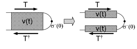
Figure 3.1: The general path integral of $\langle\sigma^{-}(t)\rangle$ has a complicated average that connects forward and backward Keldyish time contours (left). Neglecting the transitions, simplifies the integral to two independent and equal averages over each of the time directions (right).

After putting the explicit values for the Hamiltonian $H=-\sqrt{\Delta^{2}+(\varepsilon+v(t))^{2}}\sigma_{z}/2$, and noting that $\sigma_{z}$ and $\sigma^{-}$ anti-commute, we can define the factor $F(t)$ that describes the time-dependent, low frequency suppression of coherence between the two states as

$$F(t)\equiv\frac{\sigma^{-}(t)}{\sigma^{-}(0)}=\left\langle\exp\left(-i\int_{0}^{t}dt^{\prime}\sqrt{\Delta^{2}+(\varepsilon+v(t^{\prime}))^{2}}\right)\right\rangle.$$ (3.4)

If $v_{0}\ll\Delta$, one can determine the rate of accumulation of this phase by expanding the energies up to the second order in noise amplitude $v(t)$, i.e. $\sqrt{\Delta^{2}+(\varepsilon+v(t))^{2}}=\Omega+(\varepsilon v(t^{\prime}))/\Omega+(\Delta^{2}v^{2}(t^{\prime}))/(2\Omega^{3}),\;\;\Omega^{2}=\Delta^{2}+\varepsilon^{2}$, and evaluating (3.4) in the interaction representation. The pure dephasing term is:

$$F(t)=\left\langle\exp\left\{-i\int_{0}^{t}\left[\frac{\varepsilon v(t^{\prime})}{\Omega}+\frac{\Delta^{2}v^{2}(t^{\prime})}{2\Omega^{3}}\right]dt^{\prime}\right\}\right\rangle\,.$$ (3.5)

For Gaussian noise, the correlation function (3.2) determines the noise statistics completely. In this case, it is convenient to take the average in equation (3.5) by writing it as a functional integral over noise. For this purpose, we start with the “transition” probability $p(v_{1},v_{2},\delta t)$ [60, 61] for the noise to have the value $v_{2}$ time $\delta t$ after it had the value $v_{1}$:

$$p(v_{1},v_{2},\delta t)=\frac{1}{\sqrt{2\pi v_{0}^{2}(1-e^{-2\delta t/\tau})}}\exp\left\{-\frac{(v_{2}-v_{1}e^{-\delta t/\tau})^{2}}{2\pi v_{0}^{2}(1-e^{-2\delta t/\tau})}\right\}\,.$$ (3.6)

Using this expression we introduce the probability of specific noise realization as $p_{0}(v_{1})\cdot p(v_{1},v_{2},\delta t_{1})\cdot p(v_{2},v_{3},\delta t_{2})\cdot...$, where $p_{0}(v)=(2\pi v_{0}^{2})^{-1/2}\exp\{-v^{2}/2v_{0}^{2}\}$ is the stationary Gaussian probability distribution of $v$, and $\delta t_{i}$ are some small discrete time steps. Putting the explicit values for $p$’s given above with the same $\delta t$ into the formula for $F(t)$ we obtain the following expression

$$F(t) = \frac{\exp\{-v_{1}^{2}/2v_{0}^{2}\}}{(2\pi v_{0}^{2})^{(N+1)/2}(1-e^{-2\delta t/\tau})^{-N/2}}\times$$

$$\prod_{n=1}^{N}\exp\left\{-\frac{(v_{n+1}-v_{n}e^{-\delta t/\tau})^{2}}{2v_{0}^{2}(1-e^{-2\delta t/\tau})}\right\}\exp\left\{-i\delta t\left[\frac{\varepsilon v_{n}}{\Omega}+\frac{\Delta^{2}v_{n}^{2}}{2\Omega^{3}}\right]\right\}.$$

After expanding up to second non-vanishing order of $\delta t$ and taking the limit $\delta t\rightarrow 0$, the above expression can be written as $F(t)=S(\lambda)/S(1)$, where $S(\lambda)$ is the following functional integral:

$$S(\lambda) = (const)\times\frac{1}{\kappa}\int dv(0)dv(t)\mathcal{D}v(t^{\prime})$$

$$\times \exp\left\{-\frac{v(0)^{2}+v(t)^{2}}{\kappa}-\int_{0}^{z}dt(\dot{v}^{2}+v^{2}+2i\alpha v)\right\},$$

with $\kappa$, $\alpha$ and $z$ given as

$$\kappa=\left(1+\frac{2iv_{0}^{2}\Delta^{2}\tau}{\Omega^{3}}\right)^{\frac{1}{2}},\quad\alpha=\frac{\varepsilon\tau v_{0}}{\Omega\kappa^{3/2}},\quad z=\frac{\kappa t}{\tau}.$$ (3.8)

Since the average in equation (3.5) with the weight (3.1) is now given by the Gaussian integral, it can be calculated in the usual way (i.e. see [62]):

$$F(t) = F_{0}(t)\exp\left[-\alpha^{2}\left(\frac{\kappa t}{\tau}-2[\coth\frac{\kappa t}{2\tau}+\kappa]^{-1}\right)\right],$$ (3.9)

$$F_{0}(t) = e^{t/2\tau}[\cosh(\kappa t/\tau)+\frac{1+\kappa^{2}}{2\kappa}\sinh(\kappa t/\tau)]^{-1/2}.$$

3.1.1 Single Qubit Results and Conclusion

Equation (3.9) is the main analytical result for dephasing by the Gaussian noise. To analyze its implications, we start with the zero-bias, (i.e. $\varepsilon=0)$ case, where pure qubit dephasing vanishes in the standard perturbation theory. Dephasing (3.9) is still non-vanishing and its strength depends on the noise spectral density at zero frequency $S_{v}(0)=2v_{0}^{2}\tau$ expressed through $\kappa=\sqrt{1+is}$, $s\equiv S_{v}(0)/\Delta$ for convenience. The numerical simulations show that equation (3.9) and the transition contributions fully account for qubit decoherence as shown in figure 3.2. For small and large times $t$ equation (3.9) simplifies to:

$$F(t)=\left\{\begin{array}[]{cc}\displaystyle{\left[\frac{1+t/\tau}{1+t/\tau+ist/2\tau}\right]^{1/2}},&t\ll\tau\,,\\ 2\sqrt{\kappa}e^{-(\gamma+i\delta)t}/(1+\kappa)\,,&t\gg\tau\,,\end{array}\right.$$ (3.10)

where

$$\gamma=\frac{1}{2\tau}\left[\left(\frac{(1+s^{2})^{1/2}+1}{2}\right)^{1/2}-1\right]\,.$$ (3.11)

Besides suppressing the coherence, the noise also shifts the frequency of qubit oscillations. The corresponding frequency renormalization is well defined for $t\gg\tau$:

$$\delta=\frac{1}{2\tau}\left[\frac{(1+s^{2})^{1/2}-1}{2}\right]^{1/2}\,.$$

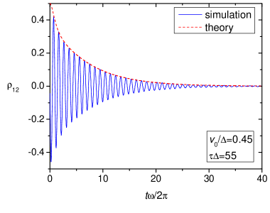
Figure 3.2: The envelope of total decoherence due to adiabatic dephasing and the transitions as predicted by equation (3.9) and the golden rule (dotted line) plotted together with Monte Carlo simulation of the quantum oscillations for the same qubit (solid line). The simulation consists of $10^{5}$ realizations over noise parameters specified on the plot.

Suppression of coherence (3.10) for $t\ll\tau$ can be qualitatively understood as the result of averaging over the static distribution of noise $v$. In contrast, at large times $t\gg\tau$, the noise appears to be $\delta$-correlated, the fact that naturally leads to the exponential decay (3.10). This interpretation means that the two regimes of decay should be generic to different models of the low-frequency noise. Indeed, they exist for the non-Gaussian noise considered [63, 64], and are also found for Gaussian noise with $1/f$ spectrum [65]. Crossover between the two regimes takes place at $t\simeq\tau$, and the absolute value of $F(t)$ in the crossover region can be estimated as $(1+s^{2})^{-1/4}$, i.e. $s$ determines the amount of coherence left to decay exponentially. The rate (3.11) of exponential decay shows a transition from the quadratic to square-root behavior as a function of $S_{v}(0)$ that can be seen in figure 3.3. The figure also shows that the decay rate extracted from numerical simulations of Gaussian noise agree well with the theoretical predictions for quite large noise amplitude $v_{0}$.

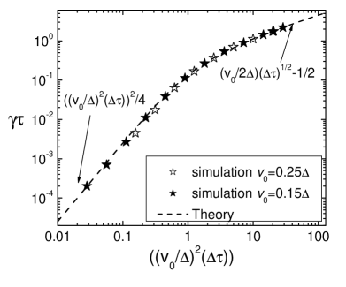
Figure 3.3: The rate $\gamma$ of exponential qubit decoherence at long times $t\gg\tau$ for $\varepsilon=0$ and noise with characteristic amplitude $v_{0}$ and correlation time $\tau$. Solid line gives analytical results: Eq. (3.11) . Symbols show $\gamma$ extracted from Monte Carlo simulations of qubit dynamics. Going from left to right along the horizontal axes the number of Monte Carlo realizations gradually changes from $10^{7}$ to $10^{4}$. Inset shows schematic diagram of qubit basis states fluctuating under the influence of noise $v(t)$.

Non-zero qubit bias $\varepsilon$ leads to the additional dephasing $F(t)/F_{0}(t)$ described by the last exponential factor in equation (3.9). The contribution from $F_{0}(t)$ is of the same form as in zero-bias case but now with the replacement $s\rightarrow s(\Delta/\Omega)^{3}$. The additional dephasing exhibits the crossover at $t\simeq\tau$ from “inhomogeneous broadening”(averaging over the static distribution of the noise $v$) to exponential decay at $t\gg\tau$. In contrast to zero-bias result, the short-time decay is now Gaussian:

$$\ln\left[\frac{F(t)}{F_{0}(t)}\right]=-\frac{\varepsilon^{2}}{\Omega^{2}}\cdot\left\{\begin{array}[]{cc}\displaystyle v_{0}^{2}t^{2}/2\,,&t\ll\tau\,,\\ v_{0}^{2}\tau t/(1+is(\Delta/\Omega)^{3})\,,&t\gg\tau\,.\end{array}\right.$$

We see again that the rate of exponential decay depends non-trivially on the noise spectral density $S_{v}(0)$, changing from direct to inverse proportionality to $S_{v}(0)$ at small and large $s$, respectively.

The approach outlined above can be used to calculate the rate of exponential decay at large times $t$ for Gaussian noise with arbitrary spectral density $S_{v}(\omega)$. Such noise can be represented as a sum of the noises (3.2) and appropriate transformation of the variables in this sum enables one to write the average over the noise as a functional integral similar to (3.1). For calculation of the relaxation rate at large $t$, the boundary terms in the integral (3.1) can be neglected. The integral is then dominated by the contribution from the “bulk” which can be conveniently written in terms of the Fourier components

$$v_{n}=(2/t)^{1/2}\int_{0}^{t}dt^{\prime}v(t^{\prime})\sin\omega_{n}t^{\prime}\,,\;\;\;\omega_{n}=\pi n/t\,,$$

and, $\langle\cdots\rangle=\int Dv\cdots\exp\{-(1/2)\sum_{n}|v_{n}|^{2}/S_{v}(\omega_{n})\}$. Combining this equation and equation (3.5) we get at large $t$:

$$F(t)=\exp\left\{-\frac{t}{2}\left[\frac{\varepsilon^{2}\Omega S_{v}(0)}{\Omega^{3}+iS_{v}(0)\Delta^{2}}+\frac{1}{\pi}\int_{0}^{\infty}d\omega\ln\left(1+i\frac{S_{v}(\omega)\Delta^{2}}{\Omega^{3}}\right)\right]\right\}\,.$$ (3.12)

For unbiased qubit, $\varepsilon=0$, this equation coincides with the one obtained by a more involved diagrammatic perturbation theory in quadratic coupling [65].

3.2 Double Qubit

Now we proceed to determine the adiabatic dephasing decoherence rate for a coupled qubit system operating at the co-resonance point. As described earlier the model double-qubit Hamiltonian at co-resonance point is:

$$H_{0}=\hbar\sum_{j=1,2}\Delta_{j}\sigma_{x}^{(j)}+\hbar\nu\sigma_{z}^{(1)}\sigma_{z}^{(2)}+\hbar\sum_{j=1,2}v_{j}(t)\sigma_{z}^{(j)},$$ (3.13)

where again $\sigma$’s denote the Pauli matrices, $\nu$ is the qubit interaction energy, $\Delta_{j}$ are the tunnelling amplitudes of the two qubits, and $v_{j}$ are two weakly coupled, in general correlated noise sources. As it can be seen from figure 2.1, applying the idea of pure dephasing being dependent on noise induced variation of the energy splitting between the levels of interest, is simplified at the co-resonance point by the vanishing linear dependence between the energy levels and the noise parameters $v_{1,2}$.

After following the same arguments as for the single qubit case of neglecting the transition rates and only concentrating on the variation of energy splitting between the corresponding energy levels, the general expression for pure dephasing expressed a path integral in the interaction picture is:

$$\frac{\rho_{ij}(t)}{\rho_{ij}(0)} = \left\langle\exp\left\{i\sum_{m,n=1,2}\int_{0}^{t}dt^{\prime}v_{m}c_{mn}^{(ij)}v_{n}\right\}\right\rangle_{v_{1},v_{2}}$$ (3.14)

$$(ij) \in \{(13),(14),(32),(42)\},$$

where $c_{n,m}^{(ij)}$ are elements of $2\times 2$ symmetric matrix describing the dependence of the energy splitting as a function of noise sources obtained by Taylor expansion

$$c_{n,m}^{(ij)}=\frac{1}{2\hbar}\frac{\partial^{2}(E_{i}-E_{j})}{\partial v_{m}\partial v_{n}}.$$ (3.15)

The averaging in (3.14) is now done over two noise sources whose dependence on integration variable $t^{\prime}$ is implied.

The analytic values of the coefficients (3.15) can be easily obtained with the help of the perturbation theory. As expected from the vanishing first-order energy variations at the co-resonance point, the first-order corrections to energy vanish, i.e.

$$\frac{\partial E_{i}}{\partial v_{1,2}}=\left\langle\psi_{i}\left|\frac{\partial H}{\partial v_{1,2}}\right|\psi_{i}\right\rangle=0.$$

The second order deviation in energy is non-vanishing, and it can be shown that

$$\frac{\partial^{2}E_{i}}{\partial v_{n}\partial v_{m}}=2\sum_{j\neq i}\frac{\langle\psi_{i}|\sigma_{z}^{(n)}|\psi_{j}\rangle\langle\psi_{j}|\sigma_{z}^{(m)}|\psi_{i}\rangle}{E_{i}-E_{j}},$$

where the wave functions are defined in (2.7). The coefficients of four $c^{(ij)}$ matrices are explicitly given in table 3.1.

$(ij)$	$c^{(ij)}_{11}$	$c^{(ij)}_{22}$	$c^{(ij)}_{12}$
$(13)$	$\displaystyle\frac{\epsilon\Omega-\delta\Delta+\nu^{2}}{\epsilon\Omega(\Omega-\epsilon)}$	$\displaystyle\frac{\epsilon\Omega+\delta\Delta+\nu^{2}}{\epsilon\Omega(\Omega-\epsilon)}$	$\displaystyle\frac{4\nu}{\Delta^{2}-\delta^{2}}$
$(42)$	$\displaystyle\frac{\epsilon\Omega+\delta\Delta-\nu^{2}}{\epsilon\Omega(\Omega-\epsilon)}$	$\displaystyle\frac{\epsilon\Omega-\delta\Delta-\nu^{2}}{\epsilon\Omega(\Omega-\epsilon)}$	$\displaystyle-\frac{4\nu}{\Delta^{2}-\delta^{2}}$
$(32)$	$\displaystyle\frac{\epsilon\Omega+\delta\Delta-\nu^{2}}{\epsilon\Omega(\Omega+\epsilon)}$	$\displaystyle\frac{\epsilon\Omega-\delta\Delta-\nu^{2}}{\epsilon\Omega(\Omega+\epsilon)}$	$-\displaystyle\frac{4\nu}{\Delta^{2}-\delta^{2}}$
$(14)$	$\displaystyle\frac{\epsilon\Omega-\delta\Delta+\nu^{2}}{\epsilon\Omega(\Omega+\epsilon)}$	$\displaystyle\frac{\epsilon\Omega+\delta\Delta+\nu^{2}}{\epsilon\Omega(\Omega+\epsilon)}$	$\displaystyle\frac{4\nu}{\Delta^{2}-\delta^{2}}$

Table 3.1: The coefficients of symmetric $2\times 2$ matrix $c^{(ij)}$ for four different density matrix elements $\rho_{ij}$.

Lastly, we are left to discus the complications that arise in evaluation of the expression (3.14) due to the correlation between the noise sources $v_{1}$ and $v_{2}$. In general, correlation between any two stochastic processes can symmetrically be expressed through a coefficient $\lambda$ such that

$$v_{1}(t) = \frac{1}{\sqrt{2}}\left(\sqrt{1+\lambda}\,\tilde{v}_{1}(t)+\sqrt{1-\lambda}\,\tilde{v}_{2}(t)\right),$$ (3.16)

$$v_{2}(t) = \frac{1}{\sqrt{2}}\left(\sqrt{1+\lambda}\,\tilde{v}_{1}(t)-\sqrt{1-\lambda}\,\tilde{v}_{2}(t)\right),$$

where $\tilde{v}_{1,2}$ are two uncorrelated noise sources, i.e. $\langle\tilde{v}_{1}(t)\tilde{v}_{2}(0)\rangle=0$. Therefore, after an appropriate orthogonal transformation (3.16), any averaging over two correlated noise sources can be expressed as averaging over two uncorrelated sources.

Assuming that the two noise sources $\tilde{v}_{1,2}$ are identical, then $\langle\tilde{v}_{1}(t)\tilde{v}_{1}\rangle=\langle\tilde{v}_{2}(t)\tilde{v}_{2}\rangle=v_{0}^{2}e^{-|t|/\tau}$, and the final expression for adiabatic dephasing of the density matrix elements needed to calculate the two probability values $p_{1,2}(t)$ defined in (2.14) is:

$$\frac{\rho_{ij}(t)}{\rho_{ij}(0)} = \left\langle\exp\left(\frac{i}{2}\sum_{m,n=1,2}\tilde{v}_{m}C_{mn}^{(ij)}\tilde{v}_{n}\right)\right\rangle_{\tilde{v}_{1,2}}$$ (3.17)

$$(ij) \in \{(13),(14),(32),(42)\},$$

where

$$C_{11}^{(ij)} = (c^{(ij)}_{11}+c^{(ij)}_{22}+2c^{(ij)}_{12})(1+\lambda),$$

$$C_{22}^{(ij)} = (c^{(ij)}_{11}+c^{(ij)}_{22}-2c^{(ij)}_{12})(1-\lambda),$$

$$C_{12}^{(ij)} = C_{21}^{(ij)}=(c^{(ij)}_{11}-c^{(ij)}_{22})\sqrt{1-\lambda^{2}}\;.$$

Each noise source is fully described by conditional probability (3.6), and the averaging (3.17) is straight forward along the lines of single qubit case. The un-normalized action is:

$$S(\hat{C}^{(ij)})=(const)\times$$

$$\int\prod_{m=1,2}d\tilde{v}_{m}(0)d\tilde{v}_{m}(t)\mathcal{D}\tilde{v}_{m}\exp\left\{-\sum_{m=1,2}\frac{\tilde{v}^{2}_{m}(0)+\tilde{v}^{2}_{m}(t)}{4v_{0}^{2}}\right\}\times$$

$$\exp\left\{-\frac{\tau}{4v^{2}_{0}}\int_{0}^{t}dt^{\prime}\left[\sum_{m=1,2}\left(\dot{\tilde{v}}_{m}^{2}+\frac{\tilde{v}_{m}^{2}}{\tau^{2}}\right)+\frac{2iv^{2}_{0}}{\tau}\sum_{m,n=1,2}\tilde{v}_{m}\hat{C}_{mn}^{(ij)}\tilde{v}_{n}\right]\right\}.$$

An orthogonal transformation, $\tilde{v}_{1,2}\rightarrow v_{1,2}$ that diagonalizes the matrix $C^{(ij)}$ decouples (3.2) into two quadratic integrals identical to those of optimally biased qubit (3.9), where $\kappa^{(ij)}_{1,2}$ are in this case the functions of $c^{(ij)}_{1,2}$ - i.e. the eigenvalues of matrix $C^{(ij)}$. The constant term in each of the two integrals over the paths $\mathcal{D}[\tilde{v}]$ get divided out by the normalizing terms consisting of interaction free action (3.2), i.e. $S(\textbf{1}_{2\times 2})$. All put together, the adiabatic contribution to dephasing of double qubit system operating at co-resonant point is:

$$\frac{\rho_{ij}(t)}{\rho_{ij}(0)} = F_{0}(t,\kappa^{(ij)}_{1})F_{0}(t,\kappa^{(ij)}_{2}),$$ (3.19)

$$F_{0}(t,\kappa^{(ij)}_{k}) = e^{t/2\tau}\left[\cosh(\kappa^{(ij)}_{k}t/\tau)+\frac{1+(\kappa^{(ij)}_{k})^{2}}{2\kappa^{(ij)}_{k}}\sinh(\kappa^{(ij)}_{k}t/\tau)\right]^{-1/2},$$

$$\kappa^{(ij)}_{1,2} = \sqrt{1+2i\tau v^{2}_{0}c^{(ij)}_{1,2}},$$

$$c^{(ij)}_{1,2} = (c^{(ij)}_{11}+c^{(ij)}_{22}+2\lambda c^{(ij)}_{12})\pm$$

$$\left[(c^{(ij)}_{11}+c^{(ij)}_{22}+2\lambda c^{(ij)}_{12})^{2}-4(1-\lambda^{2})(c^{(ij)}_{11}c^{(ij)}_{22}-(c^{(ij)}_{12})^{2})\right]^{1/2},$$

$$(ij) \in \{(13),(14),(32),(42)\}.$$

The expressions from the table 3.1 yield the following eigenvalues $c^{(ij)}_{1,2}$:

$$c^{(13)}_{1,2} = A\pm\sqrt{A^{2}-4(1-\lambda^{2})B}\;,$$

$$A = 2\left[\frac{1}{\Omega-\epsilon}\left(1+\frac{\nu^{2}}{\epsilon\Omega}\right)+\frac{4\lambda\nu}{\Delta^{2}-\delta^{2}}\right],$$

$$B = \frac{1}{(\Omega-\epsilon)^{2}}\left[\left(1+\frac{\nu^{2}}{\epsilon\Omega}\right)^{2}-\frac{\Delta^{2}\delta^{2}}{\epsilon^{2}\Omega^{2}}\right]-\frac{\nu^{2}}{(\Delta^{2}-\delta^{2})^{2}},$$

$c^{(42)}_{1,2}\equiv c^{(13)}_{1,2}$ with $\nu\rightarrow-\nu$,

$$c^{(14)}_{1,2} = a\pm\sqrt{a^{2}-4(1-\lambda^{2})b}\;,$$

$$a = 2\left[\frac{1}{\Omega+\epsilon}\left(1-\frac{\nu^{2}}{\epsilon\Omega}\right)+\frac{4\lambda\nu}{\Delta^{2}-\delta^{2}}\right],$$

$$b = \frac{1}{(\Omega+\epsilon)^{2}}\left[\left(1-\frac{\nu^{2}}{\epsilon\Omega}\right)^{2}-\frac{\Delta^{2}\delta^{2}}{\epsilon^{2}\Omega^{2}}\right]-\frac{\nu^{2}}{(\Delta^{2}-\delta^{2})^{2}},$$

and $c^{(32)}_{1,2}\equiv c^{(14)}_{1,2}$ with $\nu\rightarrow-\nu$.

3.2.1 Double Qubit Results and Conclusions

As we see from (3.19) the decoherence rates of the double qubit contain two contributions from the low frequency noise that are identical to the one obtained for the single qubit (3.9). Therefore, the conclusions of the single qubit carry over for the double qubit case. Specifically, there are the two regions of the decay - one when $t\ll\tau$ that is described by averaging over the statical distribution of the noise, and the other, $t\gg\tau$, where the noise appears to be delta-correlated and that is characterized by exponential decay. The expressions of the two decay coefficients at opposite time limits are given by (3.10) and (3.11). Numerical simulations of the coupled qubit dynamics show very good agreement with the theoretical predictions of the decoherence rates as shown in the figure 3.4.

Figure 3.4: Log plot of numerical Monte Carlo simulations (solid lines) and theoretical decay predictions $\Gamma_{TH}$(dashed lines) for evolution of $|\rho_{13}|$ density matrix element for a coupled qubit operating at co-resonance point and with two noises exhibiting different levels of correlation ($\lambda=0,0.5,$ and $1)$. The decay rates $\Gamma_{TH}$ are sum of high-f contributions from equations (2.20) and (2.21) and low-f contributions (3.19) in the limit $t\gg\tau$ as given by (3.11). For the plots $\Delta=5\nu$, $\delta=3\nu$, $\tau=100/\nu$, and initial condition $|\Psi(0)\rangle=|00\rangle$, while the MC simulations consist of $10^{5}$ realizations.

Although the double qubit system contains twice as many terms that suppress its coherent oscillations, we have to be careful not to understate the importance the rearrangement of the energy spectrum plays in the relative values of these coefficients and naively assert that the double system decoherence rate doubles as compared to the system’s individual qubit decoherence rates. This dependence is rather non-trivial even under all the assumptions about the system and the noise considered so far.

To illustrate this point we will consider the experiment [20]. Under the assumption of uncorrelated, identical baths, the low-f dephasing terms will be the same for qubit density matrix elements (13) and (42) as well as for the terms (32) and (14). At this point, it is advantageous to define a coefficient which represent the ratio of the large-time, ($t\gg\tau$), decoherence rates of the coupled qubit density matrix elements $\rho_{ij}$ to the decoherence rates of the two individual, uncoupled qubits $k=1,2$:

$$R^{(ij)}_{k}=\frac{\gamma(S(0)c^{(ij)}_{1})+\gamma(S(0)c^{(ij)}_{2})}{\gamma(S(0)/\Delta_{k})},$$ (3.20)

$$\gamma(s)=\frac{1}{2\tau}\left[\left(\frac{(1+s^{2})^{1/2}+1}{2}\right)^{1/2}-1\right],$$

$$(ij)\in\{(13),(14),(23),(24)\},\quad k=1,2,$$

where $c^{(ij)}_{1,2}$ are given in (3.19) and $\Delta_{k}$ are individual qubit tunneling amplitudes. The the eight ratios (3.20) with the parameters given in [20] are plotted in figure 3.5 as functions of zero-frequency noise spectral density, $S(0)$, in the units of $\Delta=\Delta_{1}+\Delta_{2}$. The factor-of-four increase in decoherence that was observed in the experiment can be explained by the ”numerical coincidence” of zero-frequency noise spectral density being in the range that enhances the decoherence rates of the coupled qubits.

The exact value of ratios (3.20) for the experiment [20] can be confirmed by determining $S(0)$. Since the tunneling amplitudes of the qubits are different, the value of $S(0)$ within this limit of the model can be extracted from any two, out of two $T_{1}$ and two $T_{2}$ times. Furthermore, if only the times of the same type are known, i.e. both $T_{1}$ or both $T_{2}$, they need to be measured precise enough so that their difference shows outside the margin of error. Unfortunately [20] provides only the two $T_{2}$ times that are the same within the margin of error and the exact ratio (3.20) cannot be determined.

Figure 3.5: The ratio of low-f decoherence rates with the parameters taken from experiment [20] and plotted as function of $S(0)/\Delta$, where $\Delta=\Delta_{1}+\Delta_{2}.$ The non-trivial relation between the change in the ratio of the decoherence rates between coupled and individual qubits in a double qubit Hamiltonian is evident. The expected factor-of-two increase of the decoherence rates of the coupled qubit as compared to the single qubit is not realized. Rather, it can vary over a much larger range.

In summary, the non-perturbative treatment of the now-f noise from a fluctuators coupled to the basis-forming degrees of freedom has provided the analytical expressions which can fully within this model account for the increase of the decoherence rate beyond the predictions of Fermi’s Golden Rule. In general, this is attributed to the accumulation of the phase in the qubit due to adiabatic low-f variations of the bias. Furthermore, the factor-of-four increase of decoherence rate of coupled qubits as compared to the individual qubits [20] can be attributed to changes of the energy spectrum of the system when the two qubits are coupled as supposed when they are not. This supports ”numerical coincidence” explanation to the decoherence rate increase rather than the existence of new decoherence mechanism. All the results have been verified numerically.

Chapter 4 Realistic Quantum Modelling of Systems Subject to General Noise

The ideas of adiabatic dephasing depending on the variation of the energy level spacing as the function of coupled weak noise and the transition rates being influenced by the value of spectral density of the noise at resonant frequency can be extended to a general n-qubit case in order to determine the desired decoherence rates of the system. Never-the-less, obtaining analytical results forces often a general system to be constrained in many ways such as operating at particular Hamiltonian constant in time and subject to specific, analytic noise spectral density.

The realistic applications often call for insights in to the dynamics of the system with time-varying parameters and subject to multiple noise sources described by some general spectral densities. In order to arrive to the result under these quite general conditions, it is necessary to abandon analytical expressions that were useful in qualitative understanding of the noise and resort to numerical simulations. The statistical nature of noise makes Monte Carlo (MC) methods ideal in realizing these simulations.

4.1 Simulating the Basic Qubit Dynamics

In the simulation of the qubit evolution all the time-dependent qubit ($\varepsilon,\Delta$) and noise ($v,u$) parameters of the system Hamiltonian

$$H(t)=-\frac{1}{2}\left[(\varepsilon(t)+v(t))\sigma_{z}+(\Delta(t)+u(t))\sigma_{x}\right],$$ (4.1)

are considered constant during a given time step $\delta t$, and the evolution of the qubit’s density matrix $\rho$ can be calculated exactly during the time interval:

$$\rho(t_{n}+\delta t)=\exp(-i\delta tH_{n}/\hbar)\rho(t_{n})\exp(i\delta tH^{\dagger}_{n}/\hbar),$$ (4.2)

where $H_{n}\equiv H(t_{n})$. At the boundary, the final values of density matrix are used as initial values of density matrix for the next interval with up-to-date parameters,

$$\rho(t_{n+1},H_{n+1})=\rho(t_{n}+\delta t,H_{n}).$$ (4.3)

Repeating this process eventually evolves an initially specified density matrix of a qubit to some final value along the path specified by deterministic Hamiltonian and a random realization of each of the noises. Restarting this process over many different realizations of the noises and averaging the density matrix of the system at each time point yields complete time-evolved MC-evaluated density matrix of the system.

The uncertainty of the averaged $\rho(t)$ can be attributed to three sources: (1) computer truncation, (2) the assumption of constant parameters at the discrete time steps and, (3) statistical uncertainty due to the Monte Carlo averaging.

Since the density matrix parameters are all on the order of unity the truncation error is at least sixteen orders of magnitude smaller. Its accumulation does not pose any serious problems since it is not compounded over the different realizations and at the extreme one realization has $10^{10}$ calculations. Thus even in the worst case, the result will contain error that is six orders of magnitude smaller and therefore negligible.

The error due to the discretization of the qubit parameters during the interval $\delta t$ is more serious because of the possibility of having unstable time step $\delta t$. This would lead to numerical result diverging away from the exact, unknown value. The most direct way to improve on this error is to reduce $\delta t$ or use a mid-point or some more elaborate extrapolating method when converting the continuous parameters to discrete ones. In the case of unstable time step $\delta t$, the simulation of the system without noise would produce density matrix exhibiting non-unitary behavior. For this reason, a very good check for an adequate choice of $\delta t$ consists of evolving the system without the noise forward in time from $\rho(0)$ to $\rho(t_{final})$, then reversing the time parameter, (i.e. $\delta t\rightarrow-\delta t$), and evolving $\rho(t_{final})$ backward in time to $\tilde{\rho}(0)$. The unitarity of quantum mechanics implies that the two matrices $\rho(0)$ and $\tilde{\rho}(0)$ should be identical if $\delta t$ is chosen appropriately.

With $\delta t$ chosen such that $\rho(0)=\tilde{\rho}(0)$ the only error in the result comes form the uncertainty due to Monte Carlo averaging. This error is given as

$$\Delta(\rho_{ij}(t_{n}))=\sqrt{\frac{\langle\langle\rho^{2}_{ij}(t_{n})\rangle\rangle-\langle\langle\rho_{ij}(t_{n})\rangle\rangle^{2}}{N}},$$ (4.4)

where $N$ is the number of realizations, and the double-angled brackets denote arithmetic average over the realizations [66]. Taking into account that the elements of density matrix are on the order of unity, the error due MC averaging can be made reasonably small by increasing the number of realizations.

The non-trivial nature of generating the noise form a given spectral density of its correlator does not allow the improvement to the variance (4.4) by utilization of stratified or importance sampling techniques. The $1/\sqrt{N}$ reduction of the variance can be improved by using the antithetic technique or by employing quasi-random sampling. The antithetic technique [67] is implemented by using a single realization of the noise twice - once as generated by random precess and second time reused but with opposite sign. The quasi-random sampling assures better covering of the sample space by generating the random numbers with the help of number theory that assures the ”filling” of the empty space between already sampled ”random” points. This method can reduce the $1/\sqrt{N}$ dependence to $1/N$ [66].

4.2 Generating Noise

Unlike in the case of previous qubits, the numeric Hamiltonian (4.1) has noises affecting both the tunneling and the bias of the qubit. This is often the case in the realistic situations. For instance in the experiment [30] the tunneling noise can be attributed to the impurities in the layer separating the superconducting electrodes of the Josephson junctions or to the variations in the modulating flux $\Phi_{xd.c.}$ as defined in figure 1.3. In the same experiment the bias noise originates form the variations in the applied flux $\Phi_{x}$ and from the dc-SQUID magnetometer. With exception to the impurity caused noise, the noises caused by the sources above are in general specified by some noise spectral densities $S_{i}(\omega)$ obtained form the known impedances of the circuits $Y_{i}(\omega)$ and the fluctuation-dissipation theorem [11]. Thus, the random noise in the qubit simulation must be generated in a way that it matches the given spectral density. Since the significant portion of noise comes from the detector, which is usually coupled to the basis forming degree(s) of freedom of the qubit, the discussion that follows assumes that the only noise affecting qubit is coupled through $z$ component so that $u\equiv 0$ in (4.5).

As discussed in [68], the random variable $v(t_{m})$ generated from some given $S(\omega)$ as

$$v(m\Delta t)=\sum_{n=0}^{M}\sqrt{4S(n\delta\omega)\delta\omega}\cos(n\delta\omega m\Delta t+\phi_{n}),\quad m=0..M,$$ (4.5)

is a Gaussian, and in the limit $N\rightarrow\infty$ it has a correlator whose spectral density is $S(\omega)$. In the equation (4.5), $\delta\omega=1/(M\Delta t)$ is discrete frequency interval while $\phi_{n}$ are uniformly distributed random phases taken randomly from the interval $[0,2\pi)$. In the numerical implementation of the same equation, the Fourier transform is replaced by fast Fourier transform (FFT). In doing so, it is important to choose $M$ and $\Delta t$ so that the cutoff time $(M\Delta t)$ is larger than the desired simulation time, and the cutoff frequency $\omega_{c}$ exceeds the qubits maximal transition frequency. It is easily shown that $\omega_{c}=1/\Delta t$ [66]. Furthermore, in order to avoid numerical aliasing caused by approximating Fourier transform by FFT it is necessary to set the cutoff to be factor-of-two larger than the maximal level spacing of the qubit $\Omega_{max}$ [66, 69].

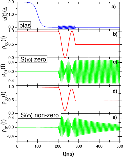
Figure 4.1: Hadamard transformation modelled by varying the bias as depicted in the graph a). The plots b) and c) show the variation of the respective density elements without noise while the plots d) and e) show the same evolution subject to noise. The simulation assumes $\Delta$ to be constant, while $S(\omega)$ was supplied numerically.

The discrete Fourier transform given in (4.5) can be expressed as a real part of more general complex transform

$$z(m\Delta t)=\sum_{n=0}^{M}\left[\sqrt{4S(n\delta\omega)\delta\omega}\exp(i\phi_{n})\right]\exp(-inm/M),\quad m=0..M,$$ (4.6)

where the random phase is now included in the harmonic coefficient. This way written transform is more favorable for FFT computation because the random phase can be factored out. Also, real and imaginary parts of noise $z(m\Delta t)$ are uncorrelated since $\cos(nx)$ and $sin(mx)$ are two orthogonal functions. Preforming one complex FFT yields two realizations of the noise, thus speeding up the simulation significantly. The antithetic variance reduction technique discussed earlier is used at this point in which case there are total of four noise realizations after single fourier transform (4.6).

Lastly the noise realization given in the time steps of $\Delta t$ needs to be expressed in the steps of the simulation $\delta t$. This can be achieved along the same lines of discretization of the continuous parameters of the Hamiltonian (4.5) discussed at the beginning of this chapter.

The approach outlined so far is very powerful, and it can produce results impossible to produce by analytical methods. Hadamard transform of a qubit state is a such example, and it’s simulation shown in the figure 4.1.

4.3 Inclusion of Temperature

Up to this point the temperature has not entered into the discussion, so the noise affecting the qubit is high-temperature noise with $k_{B}T/\hbar\gg\Delta,\varepsilon$. This implies that noise-induced up and down transition rates are the same. Realistically this is not the case since qubit experiments are performed on temperature scales of the order of $10mK\ll\Delta,\varepsilon$, where the up rate is severely suppressed.

As shown in the second chapter, the transitions are easily treated by perturbation theory and they depend on the high-frequency part of the spectral density. Thus truncating the spectral density at the frequencies larger than some frequency $\omega_{tr}$ that is on the order and also below minimal qubit level spacing $\Omega_{min}$ (figure 4.2) eliminates the transitions from the simulation as shown in figure 4.3. It is important to realize here that although the values of spectral density above the truncation frequency are zero, the value $\Delta t=1/\omega_{c}$ in (4.6) stays fixed. If this was not the case, the removal of the transition frequencies form the generated noise will not be complete because it will contain aliased contribution. Aliasing is a serious problem in the signal processing [69]. The best way to assure that the aliasing is negligible while at the same time keeping in mind that increasing cut-off is prolonging the computation time, is to pick up lowest cut-off frequency of the noise spectrum for which the truncated spectral density produces no energy relaxation, i.e. $T_{1}\rightarrow\infty$.

Since the analytic expressions for the decay rates that obey the detailed balance relation are known (e.g. see [70]), the temperature dependent transitions are accounted for after adding- in ”by hand” the appropriate coefficients in the equation (4.2).

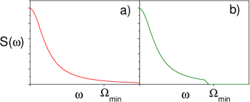
Figure 4.2: In order to eliminate transitions from the simulation the original spectral density a) needs to be truncated at the higher frequencies $\omega_{tr}\lesssim\Omega_{min}$ b).

Working explicitly in the interaction basis of the qubit, the diagonal density matrix elements acquire ”by hand” inserted decay that restores the transitions removed by the truncation of the spectral density. The same can be said about the high-f decay component of the off-diagonal matrix element. Unlike before, the restored transition rates can be made to obey the detailed balance relation with an arbitrary temperature. The explicit modifications to the equation (4.2) are:

$$\rho^{d}_{00}(t_{n}+\delta t) = \frac{\gamma_{d}}{\gamma_{u}+\gamma_{d}}+\rho^{d}_{00}(t_{n})\exp[-(\gamma_{u}+\gamma_{d})\delta t]$$ (4.7)

$$\rho^{d}_{01}(t_{n}+\delta t) = \rho^{d}_{01}(t_{n})\exp\left[-\left(i\Omega+\frac{\gamma_{u}+\gamma_{d}}{2}\right)\delta t\right].$$ (4.8)

The rates are given as

$$\gamma_{d}=\frac{\Delta}{2\Omega}S(\Omega),\quad\gamma_{u}=e^{-k_{B}T(\Omega)/\Omega\hbar}\gamma_{d},$$ (4.9)

where $T(\Omega)$ is effective temperature defined through FDT as

$$S(\omega)=Re(Y(\omega))\frac{\hbar\omega}{2\pi}\coth\frac{\hbar\omega}{2k_{B}T(\omega)}.$$ (4.10)

The inclusion of temperature requires additional specification of effective temperature $T(\omega)$ or environmental resistance $Re(Y(\omega))$ over the transition frequency range.

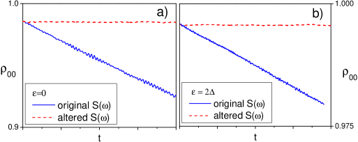
Figure 4.3: Two simulations with bias a) $\varepsilon=0$ and b) $\varepsilon=2\Delta$ each run with original (solid line) and truncated (dashed line) spectral densities. The lack of the relaxation, a phenomenon solely caused by transitions, is apparent for truncated spectral density, while the relaxation is present in the simulation with original spectral density.

.

The identical simulations run at various temperatures exhibit increasing decoherence rates with the increase of the effective temperature. The figure 4.4 shows temperature dependence of Rabi oscillations of excited qubit state caused by the rf-pumping (insert). The direct relation between temperature and the degradation of coherent oscillations is obvious.

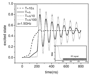
Figure 4.4: Plot of Rabi oscillations at the optimal point $(\varepsilon=0)$ simulated with different temperature values and the same rf-varied bias (insert).

4.4 Generalization to Larger Systems of Qubits

The method outlined above for simulating the dynamics of qubit can be extended to more complex qubit systems under the influence of classical noise. Inclusion of the temperature dependent transitions like as done above is impossible since the perturbative analytic expression for time decay of the system’s density matrix elements do not exist. In addition, the dimension of the Hilbert space scales exponentially $(2^{N})$ to the number of the qubits $N$, and the density matrix approach is increasingly inefficient due to need for multiple, large-matrix multiplications. These shortcomings could be overcome by use of stochastic wave function approach [71, 72, 73, 74, 75] that is unfortunately beyond this work.

Part II Quantum Measurement

Chapter 5 Continuous Weak Measurement with Mesoscopic Detectors

5.1 Quantum Measurement and Mesoscopic Detectors

Textbook examples of quantum measurements often recall the Stern-Gerlach experiment where the measured phenomenon is quantum mechanical in nature, but the measurement itself is purely classical and could only determine the amplitudes of the system’s wave function if repeated on a large number of identically prepared systems. This is a direct consequence of the design of the measuring equipment where the measured system, i.e. the beam of the electrons, is absorbed by the detector - a photographic plate or florescent screen. For this reason, the quantum state is always destroyed by the measurement.

These destructive measurements are not general representative of the quantum measurement process as formulated by von-Neuman and the others [76, 77, 78, 79, 80]. The postulate of quantum measurement asserts that the measurement of an observable quantity $q$ which gives a value $q_{j}$ leaves the density matrix of the measured system $\rho$ in the state

$$\frac{1}{Tr\{|q_{j}\rangle\langle q_{j}|\rho\}}|q_{j}\rangle\langle q_{j}|\rho|q_{j}\rangle\langle q_{j}|,$$ (5.1)

where $|q_{j}\rangle$ is the wave function of the corresponding measured value $q_{j}$ and the tracing in the denominator is done over both systems. Thus, measuring a general quantum state of a system and obtaining some result $q_{j}$ reduces the density matrix of the measured system in a way that the obtained result is now incorporated into the total, updated density matrix, where $|q_{j}\rangle$ are defined by the detector-system coupling.

In practice, the detector needs to be capable of measuring the state of the system while being at the same time minimally detrimental to the measured system’s coherence. Since the coherence is purely quantum phenomenon, its preservation imposes necessity of measuring the quantum system by entangling it with another system that also exhibits some form of dynamics on the same energy scale. Furthermore, the need of having the result in the form of a classical, measurable signal makes mesoscopic phenomenon such as Coulomb blockade or mesoscopic transport in single or multichannel conductors prime candidates for a such task.

By entangling a such mesoscopic detector with the measured system, the observation of a detector outcome does not need to destroy the measured system. If the detector is perfect, the reduction of the measured system’s matrix is given by (5.1). In general, the detector can act back onto the quantum system and the general state after the measurement can be represented as

$$\frac{1}{Tr\{|q_{j}\rangle\langle q_{j}|\rho_{sys}\}}\hat{\Omega}(q_{j})\rho_{sys}\hat{\Omega}^{{\dagger}}(q_{j}),$$ (5.2)

where $\Omega(q_{j})$ describes the total back action of the detector on the measured system. If $\Omega(q_{j})\equiv|q_{j}\rangle\langle q_{j}|$ density matrix of the measured system will remain pure and the detector will be preforming in ideal or quantum-limited regime. The exact form of the operators $\Omega(q_{j})$ depends on the type of the detector.

If the measurement outcomes are orthogonal, i.e. $|q_{i}\rangle\langle q_{j}|=\delta_{ij}$ then $|q_{j}\rangle$ are eigenvectors of the measurement basis and the measurement preformed by the detector will be projective or von-Neumann measurement. Assuming the quantum limited regime for now, the state of the quantum system after the measurement of $q_{j}$ will be projected into state given in (5.1). As a consequence of reduction of the density matrix and the orthogonality of $|q_{i}\rangle\langle q_{j}|$, any further measurements of the same quantity will give the identical outcome.

Orthogonality condition implies the direct correlation between the quantum system and the detector. Achieving this requires strong coupling between the two, which in general induces strong detector back-action beyond the limit of the ideal measurement. Reducing the back-action of the detector on the quantum system can be achieved by making the detector-system coupling weak. This leads to imperfect correlation between the detector output and the measured observable which is reflected in non-orthogonality of the operators $|q_{i}\rangle\langle q_{j}|$. Relaxing the orthogonality constraint also implies that two successive measurements of the static quantum system do not need to give the same outcome, since two or more different outcomes can be implied by the same signal, i.e. the states $|q_{j}\rangle$ are now some superpositions of the measurement basis states. In this case the output does not tell what state was measured, but it reflects the likelihood of the system being in the states that all could with some weights belong to the observed output. The successive weak measurements of the quantum system collapse its wave function to one of the states determined by the system-detector coupling. The slow reduction of the wave function enables continuous measurement of the quantum system and avoids the possibility of abrupt energy relaxation that is characterized by projective measurements which can result in total destruction of the quantum state due to the secondary reasons [81].

A way to study weak measurement is in the framework of linear response theory where the interaction of weak detector force $f$ and the quantum system coordinate $x$ is assumed to be linear. The Hamiltonian is specified as $H=H_{q}+H_{d}+xf$, which in addition to the interaction coupling contains individual Hamiltonians of the quantum system $H_{q}$ and the mesoscopic detector $H_{d}$. Large size of the detector justifies the assumptions that the detector is static and that the changes in the detector are observable in the form of some classical output signal $o(t)$. To the first order correction, the detector output can be written as consisting of the detector’s noise $v(t)$ and measurement signal superimposed over it,

$$o(t)=v(t)+\frac{i}{\hbar}\int d\tau[f(\tau),v(t)]x(\tau).$$ (5.3)

Since different times correspond to different and independent measurements, the noise of the detector is white and is completely specified by its correlator $\langle v(t)v(t^{\prime})\rangle_{d}=2\pi S_{v}\delta(t-t^{\prime})$, where $S_{v}$ is the noise spectral density that is assumed constant at the relevant low-frequency range of the output signal. The delta function is a consequence of the instantaneous detector response. The detector acts on the measured system through the detector force $f(t)$ which induces stochastic motion to the quantum system. In this light, the correlator of the force describes the back-action of the detector, and it as well is characterized by some spectral density $S_{f}$ constant in the relevant frequency range, it responds instantaneously and is independent of its values at the different times, thus $\langle f(t)f(t^{\prime})\rangle_{d}=2\pi S_{f}\delta(t-t^{\prime})$. The average detector force component is assumed to be zero, $\langle f\rangle_{d}\equiv 0$, since any non-vanishing value can be absorbed by renormalizing the detector Hamiltonian $H_{d}$. The commutator of the cross-correlator between the noise and the detector force $i\langle[f(t^{\prime}),v(t)]\rangle_{d}=\hbar\lambda\delta(t-t^{\prime}-0)$ essentially describes the information extraction from the measured system by the detector. The infinitesimal shift in the detector response is required in order to impose the causality in (5.3).

In the case of the continuous measurement, the extraction of information from the measured system is not instantaneous but it is spread out over some time $\tau_{m}$. Complementary to the extraction of the information from the quantum system the detector’s back-action is dephasing the measured system’s wave-function. In the case of static quantum system ($H_{q}\equiv 0$), the density matrix $\rho$ of the measured system evolves in the eigenbasis of the observable $q$ as:

$$\dot{\rho}_{jj^{\prime}}=-\frac{i}{\hbar}(q_{j}-q_{j^{\prime}})f(t)\rho_{jj^{\prime}},$$ (5.4)

whose solution is given by $\rho_{jj^{\prime}}(t)=\rho_{jj^{\prime}}(0)\exp(-i(q_{j}-q_{j^{\prime}})/\hbar\int^{t}f(t^{\prime})dt^{\prime})$. After the averaging over the different realizations of $f(t)$ and using the well known result, $\langle\exp(x)\rangle=\exp\langle x^{2}/2\rangle$, the decay of the density matrix elements due to the detector back-action is:

$$\rho_{jj^{\prime}}(t)=\rho_{jj^{\prime}}(0)\exp(-\Gamma_{d}t),\quad\Gamma_{d}=\frac{\pi S_{f}(q_{j}-q_{j^{\prime}})^{2}}{\hbar^{2}}.$$ (5.5)

At the same time, the dc component of the detector output signal changes by the value $\delta o=\lambda(q_{j}-q_{j^{\prime}})$ where $\lambda$ is the detector response coefficient defined earlier. In order to read-out the output signal, the background noise needs to subside to at least the half value of the $\delta o$. Since the average background detector noise $\Delta o$ averaged over some time interval $\Delta t$ decays inversely to it as $\Delta o=(2\pi S_{v}/\Delta t)^{1/2}$, the measurement time $\tau_{m}$ is:

$$\tau_{m}=\frac{8\pi S_{v}S_{f}}{[\lambda(q_{j}-q_{j^{\prime}}))]^{2}}.$$ (5.6)

From (5.5) and (5.6) the measurement time and back-action dephasing rate $\Gamma_{d}$ are related as

$$\tau_{m}\Gamma_{d}=8(\pi/\hbar\lambda)^{2}S_{q}S_{f}.$$ (5.7)

As detailed in [12], the detector force and noise spectral densities can be defined as vector products since they are assumed constant at low frequencies:

$$S_{l}(\omega)=\frac{1}{2}\left[S_{ll}(\omega)+S_{ll}(-\omega)\right]$$

$$S_{lk}\equiv\langle l|k\rangle,\quad l,k\in\{v,f\}.$$

Then the response coefficient can be expressed as $\lambda=4\pi Im(S_{fv})/\hbar$ and the Schwartz inequality $S_{vv}S_{ff}\geq|S_{fv}|^{2}$, yields that

$$|\lambda|\leq\frac{4\pi}{\hbar}\left[S_{f}S_{v}-Re(S_{fv})^{2}\right]^{1/2}.$$ (5.8)

Combining (5.7) and (5.8) establishes a fundamental relation between the measurement time and back-action decoherence rate,

$$\tau_{m}\Gamma_{d}\geq\frac{1}{2}.$$ (5.9)

Equation (5.9) implies that the acquisition of information is never faster than the dephasing due to back-action. At best, the quantum system can be measured as fast as it is being dephased. This occurs for the detectors for which $Re[S_{fv}(\omega)]=0$, where explicitly $S_{fv}=\int d\tau exp(i\omega t)\langle fv(\tau)\rangle_{d}$. The vanishing real part of spectral density function between the noise and the back-action implies that the detector noise is not correlated with the detector force thus the detector back-action is solely caused by exchange of information and not by the detector excitations of the measured system. This-way optimized detector is known as quantum-limited or optimal detector.

5.2 Quantum Point Contact as a Detector

The discussion above can be illustrated with a specific example of quantum point contact (QPC) detector situated in the proximity of the Cooper pair box qubit. QPC is a one dimensional channel whose resistive properties in the tunneling regime are very sensitive to electric fields [83, 84, 85, 86, 87]. Therefore, the current through biased QPC is modulated by charge present in the box.

If the variations in the transmission of QPC are linear, then the detector and the interaction Hamiltonians are respectively:

$$H_{d} = \sum_{j=l,r}\sum_{i}E_{i}\hat{a}^{{\dagger}}_{ij}\hat{a}_{ij}$$ (5.10)

$$H_{i} = \frac{U}{2}\sigma_{z}\qquad U=\sum_{j,j^{\prime}=l,r}U_{jj^{\prime}}\sum_{i,i^{\prime}}\hat{a}^{{\dagger}}_{ij}\hat{a}_{i^{\prime}j^{\prime}},$$

where $\hat{a}^{{\dagger}}_{l,r}$ and $\hat{a}_{l,r}$ are electron creation and annihilation operators of the left and the right QPC electrodes, and $E_{i}$ are energies of electrons populating $i$th level. The coupling $U$ is caused by the changes in the electron scattering potential $\pm U(x)$ of QPC, where $\pm$ depends on weather the cooper pair occupies the box or not. Since the qubit is in a stationary state, its Hamiltonian is equivalent to zero. Left and right wave function of the electrons in the electrodes, $\Psi(x)_{l,r}$, define the scattering matrix elements as $U_{ij}=\int\Psi^{*}_{i}(x)U(x)\Psi_{j}(x)dx$.

Under the assumption of the QPC bias $V$ larger than the qubit parameters and the environment temperature $(eV>>\hbar\varepsilon,\hbar\Delta,k_{B}T)$, the average current passing through QPC is classical and in the zeroth order the correlators are

$$\langle U(t)U(t+\tau)\rangle = \frac{e\hbar V}{4\pi}\frac{(\delta T)^{2}+u^{2}}{TR}\delta(t)$$ (5.11)

$$\langle U(t)I(t+\tau)\rangle = \frac{e^{2}V}{2\pi}(i\delta T+u)\delta(\tau-0)$$ (5.12)

$$\langle I(t)I(t+\tau)\rangle = \frac{e^{3}VTR}{\pi\hbar}\delta(\tau)+\frac{(\delta I)^{2}}{4}\langle\sigma_{z}\sigma_{z}(t)\rangle,$$ (5.13)

where $T$ and $R$ are transmission and reflection probabilities, $\delta T$ is the change in transmission due to location of the cooper pair, while $u$ is a dimensionless parameter that does not affect the current through the contact. Rather, it reflects asymmetry of the coupling between the box and QPC [43].

The back-action dephasing can be obtained by solving an equation of motion for the reduced qubit density matrix. Since the qubit is static, only its off-diagonal elements are of interest. In this case, the transition rate through the point contact depends on the qubit state and after the averaging over $U$ as done in going form (5.5) to (5.6), the off-diagonal density matrix element of the qubit evolves according to

$$\dot{\rho}_{01}=-\Gamma_{d}\rho_{01},\quad\Gamma_{d}=\frac{eV}{\hbar}\frac{(\delta T)^{2}+u^{2}}{8\pi TR}.$$ (5.14)

The asymmetry factor $u$ does not affect the current response, therefore it has an effect of increasing decoherence rate without any increase of the data acquisition rate $\Gamma_{m}=(\delta I)^{2}/4S_{0}$, where $S_{0}\equiv 2e^{3}VTR/\pi\hbar$ is shot-noise spectral density and $\delta I=e^{2}\delta TV/\hbar\pi$[43, 88]. The ratio of two decoherence rates,

$$\frac{\Gamma_{m}}{\Gamma_{d}}=\frac{(\delta T)^{2}}{(\delta T)^{2}+u^{2}}\leq 1,$$ (5.15)

again is such that information extraction is always limited from the above by the qubit decoherence.

Since the asymmetry factor does not affect the current response, it has no effect on information extraction from the qubit. On the other hand, the qubit decoherence (5.14) is increased by non-zero $u$ and the ratio (5.15) is the most optimal for $u=0$. This illustrates the interplay of back-action decoherence and extraction of information - only ideally optimized QPC $(u=0)$ preforms quantum measurement that extracts information from the qubit as fast as it is dephasing the quantum state of the qubit by its back-action. For non-optimal case $(u\neq 0)$, a part of the information about the qubit is contained in the phase differences between the forward and backward scattering electrons in the QPC. Since this information cannot be extracted by measuring the ballistic properties of the QPC but by rather some ”elaborate”, or better said un-achievable interference between the forward and backward scattering channels, the information is lost and the QPC detector will dephase the qubit before it is able to measure its state completely. It is important to point out that the limitation (5.15) is independent of the strength of the qubit-detector coupling, rather it is an universal limitation of quantum mechanics.

5.3 Conditional Measurement

In the regime of the quantum-limited detection, the overall evolution of the detector and the measured system is quantum-coherent and the only source of the information loss is averaging over the detector. For a detector, different outcomes of the evolution are classically distinguishable, and it is meaningful to ask how the measured system evolves for a given detector output. In the quantum-limited regime, specifying definite detector output eliminates all losses of information, and as a result there is no back-action dephasing present in the dynamics of the measured system conditioned on specific detector output.

Conditional description in the quantitative form is obtained (see, e.g., [88, 71, 61]) by separating in the total wave function the terms that correspond to a specific classical outcome of measurement and renormalizing this part of the wave function so that it corresponds to the total probability of 1.

In the conditional measurement approach the measured system is specified by its wave function $|\Psi\rangle=\sum_{i}\alpha_{i}|q_{i}\rangle$. Conditional that the single detector particle was transmitted/reflected the amplitudes $\alpha_{t}$ are updated as

$$\alpha_{i}\rightarrow\frac{\alpha_{i}t_{i}}{\sqrt{\sum_{j}|\alpha_{j}t_{j}|^{2}}},\quad\alpha_{i}\rightarrow\frac{\alpha_{i}r_{i}}{\sqrt{\sum_{j}|\alpha_{j}r_{j}|^{2}}},$$ (5.16)

where $t_{i},r_{i}$ are the values of the detector transmission/reflection as functions of the state $|q_{i}\rangle$ of the measured system.

It is important to stress that the changes in the coefficients $\alpha_{i}$ for a system with vanishing Hamiltonian (as we assumed from the very beginning) is unusual from the point of view of Schrödinger equation, and provides quantitative expression of reduction of the wave function in the measurement process.

If the dynamics of the detector is not quantum limited, then the information is lost and the dephasing is non-vanishing even in conditional evolution. To generalize equations (5.16) to the case of finite dephasing, we need to look at the change of the density matrix of the measured system due to a single detector event. If the detector particle is specified as some free wave superposition $|\Psi\rangle=\int dkb(k)|k\rangle$, then after tracing out the detector degrees of freedom from the total, system-plus-detector density matrix, the density matrix $\rho_{ij}$ of the measured system changes as

$$\rho_{ij} \rightarrow \int dk|b(k)|^{2}(t_{i}(k)t^{*}_{j}(k))/\sum_{j^{\prime}}\rho_{j^{\prime}j^{\prime}}T_{j^{\prime}}$$ (5.17)

$$\rho_{ij} \rightarrow \int dk|b(k)|^{2}(r_{i}(k)r^{*}_{j}(k))/\sum_{j^{\prime}}\rho_{j^{\prime}j^{\prime}}R_{j^{\prime}}$$ (5.18)

where

$$T_{j}=\int dk|b(k)|^{2}(t_{j}(k)t^{*}_{j}(k)),\quad R_{j}=1-T_{j}$$

are total transmission and reflection probabilities for a given state $|q_{j}\rangle$ of the measured system. From these relations it is straight forward to see that quantum-limited detection requires the density matrix elements to remain pure in the conditional evolution.

5.4 Measurement of Quantum Coherent Oscillations

In order to study the measurement of the quantum coherent oscillations, the output signal correlator $\langle o(t+\tau)o(t)\rangle$ needs to be evaluated explicitly for a measured system in non-static case. In the specific example of QPC detector, the correlator is the current-current correlator given in (5.13). The first part of the expression is the contribution form the shot noise while the second part is the detector response to the qubit oscillations. To evaluate this $\langle\sigma_{z}\sigma_{z}(\tau)\rangle$ correlator, it is necessary to solve the equation of motion of the reduced density matrix of the qubit, which after substitution $\rho=1/2+\sigma$ yields:

$$\dot{\sigma}_{00}=\Delta Im[\sigma_{01}],\quad\dot{\sigma}_{01}=(i\varepsilon-\Gamma_{d})\sigma_{01}-i\Delta\sigma_{11},$$ (5.19)

where the back-action decoherence rate is given in (5.14) and the normalization condition $\sigma_{11}=-\sigma_{00}$ was used to simplify the second equation. This equation is in general solvable, and in the case of zero bias ($\varepsilon=0$), the output signal spectral density $S(\omega)=2\int\langle I(0)I(\tau)\rangle e^{i\omega\tau}d\tau$ is:

$$S(\omega)=S_{0}+\frac{\Gamma\Delta^{2}(\delta I)^{2}}{(\omega^{2}-\Delta^{2})^{2}+\Gamma^{2}\omega^{2}},$$ (5.20)

where $S_{0}\equiv 2e^{3}VTR/\pi\hbar$ is the shot noise spectral density.

The zero-bias point is the most optimal for the qubit oscillations. For this value, the spectral density is peaked at the qubit oscillation frequency $\Delta$. The maximal value of the peak above the shot noise is $S_{max}=(\delta I)^{2}/\Gamma$, and $S(\omega)$ is limited from above such that signal-to-noise ratio is

$$\frac{S_{max}}{S_{0}}=\frac{4(\delta T)^{2}}{(\delta T)^{2}+u^{2}}\leq 4.$$ (5.21)

This again illustrates the limitation between the information extraction and the back-action decoherence. In the static case the limit was exhibited through the relation between the rate of decoherence and the rate of information extraction, while in the dynamic case it is exhibited through the signal-to-nose ratio that is limited to four from above. As before, the limitation is fundamental (i.e. independent on the qubit-detector coupling). It represents the fact that in the time domain the oscillations are drowned in the detector’s shot noise.

The analytic expression for the output spectral density is possible after solving (5.19) with Cardain’s formula, but the cumbersome expressions are not very insightful. Numerical evaluations of the spectral density for finite bias qubit can be found in [88].

5.5 Quantum Non-Demolition Measurement

Even if ideally optimized, the quantum measurements discussed so far do not exceed the standard quantum limit given by (5.15) or (5.21). This is a consequence of the general choice for the system-detector coupling. For this reason, the measurement signal contains information about both conjugate variables, $[p,q]=\pm i\hbar$ of the quantum system. The Heisenberg uncertainty about them $(\Delta p\Delta q\geq\hbar/4)$, is contained in the output signal and it prevents the signal from reflecting one of them exactly.

The need to measure the mesoscopic observables beyond the quantum limit has produced a special group of measuring schemes known as quantum non-demolition (QND) measurements [89, 90, 91, 92]. They all are based on the idea of measuring only one, i.e. $q$, of the conjugate variables of the system. This way constructed detector still acts back and perturbs the unobserved conjugate variable $p$, but since the detector is only coupled to $q$ the output signal will not exhibit any consequences of the back-action on $p$. In other words the detector is coupled to the constant of motion of the measured system. Mathematically this implies that the measured observable and the operator $\hat{\Omega}(q_{i})$ defined in (5.2) commute [79],

$$[q,\hat{\Omega}(q_{i})]=0.$$ (5.22)

Specifically, in the qubit measurement discussed so far the signal-to-noise limit (5.21) of monitoring quantum coherent qubit oscillations demonstrates the inability of the measurement scheme to obtain the information about the qubit beyond the quantum limit. The origin of this limit can be traced to the nature of the qubit-detector coupling that is only sensitive to $\sigma_{z}$ projection of the qubit in some general, non-diagonal basis. For this reason, the detector is measuring directly the oscillating coordinate and consequently it localizes it. This is reflected through appearance of additional ”quantum-limiting dephasing” which constrains the signal-to-noise spectral density of the output signal to four from above. Two known ways of overcoming this obstacle and realizing the QND measurement of qubit dynamics revolve around an idea of making the qubit-detector coupling time-dependent [44, 45].

The first of the designs solves this problem on the most straight-forward way - by coupling the detector to the unbiased qubit such that the detector follows the qubit as it oscillates in $zy$-plane. If the coupling is oscillating with some frequency $\omega_{c}$ the system is described by Hamiltonian:

$$H=H_{d}-\frac{1}{2}\Delta\sigma_{x}-\frac{f}{2}\left[\cos(\omega_{c}t)\sigma_{z}+\sin(\omega_{c}t)\sigma_{y}\right].$$ (5.23)

In the regime of small detuning $\gamma$ between the measurement frame oscillation $\omega_{c}$ and the oscillation of the qubit $\Delta$, linear response language yields the spectral density of the output signal to be [44]:

$$S(\omega)=S_{0}+\frac{\lambda^{2}}{2\pi}\frac{\Gamma_{e}+\gamma}{\omega^{2}+(\Gamma_{e}+\gamma)^{2}},\quad\gamma\equiv\frac{(\omega_{c}-\Delta)^{2}}{\Gamma},$$ (5.24)

where $\lambda$ is the linear response coefficient, $\Gamma_{e}$ is the environment induced suppression of the coherence, and $\Gamma$ is the detector back-action decoherence rate. In the case of zero detuning, $\gamma=0$ and zero environment decoherence, $\Gamma_{e}=0$, the signal to noise ratio diverges for dc values of the output signal and the limit of standard quantum measurement (5.15) is surpassed.

A somewhat different scheme introduced in [45] achieves the QND measurement by employing the kicked-qubit technique where the charge qubit is coupled to QPC with the periodically switched coupling. In this case the detector has access to the qubit only at approximately discrete times. Ideally, the coupling part of the total Hamiltonian is a sequence of periodic delta functions separated by $\tau$ and of strength $f/2$,

$$H=-\frac{1}{2}\left[\varepsilon\sigma_{z}+\Delta\sigma_{x}\right]+\sum_{n=-\infty}^{\infty}\delta(t-n\tau)\frac{f(t)}{2}\sigma_{z}+H_{d}.$$ (5.25)

The density matrix of initially pure quantum state $|\Psi\rangle=\alpha|R\rangle+\beta|L\rangle$ after $n$ kicks with $\tau=2\pi/\Omega$ is

$$\rho(n)=\left(\begin{array}[]{cc}|\alpha|^{2}&Z\alpha\beta^{*}\\ Z^{*}\alpha^{*}\beta&|\beta|^{2}\\ \end{array}\right),$$ (5.26)

where $Z=exp[in\langle f\rangle-n\langle(\delta f)^{2}\rangle/2]$ is decay factor obtained by central limit theorem [93]. It is obvious that the measurement scheme is preserving the information about the $\sigma_{z}$ projection of the qubit, while the information about the remaining two projections $\sigma_{x},\sigma_{y}$ is lost. The spectral density of the detector output is discrete, but again it diverges at dc frequency value.

If the ”kicked” QND measurement technique is applied to unbiased qubit, ($H_{q}\equiv\Delta\sigma_{x}/2$), then it is possible to synchronize the measurement pulses so that the detector interacts with the qubit only when the off-diagonal elements are identical to zero. Ideally in this case, the measurement will not affect the qubit evolution at all. Realistically, the coupling is not instantaneous, and the detector interacts with the qubit when the off-diagonal elements are nearly zero. In this process, the detector induces some small relaxation still beyond quantum limit decay rate that eventually collapses the qubit. More about this will be said in the following chapter.

Chapter 6 Rapid Single Flux Detector

Many flux qubits employ the measurement scheme based on the ability of a flux qubit to modulate the rate of tunneling out of the stationary supercurrent carrying states of a Josephson junction or a SQUID. This process can be viewed as tunneling of a magnetic flux quantum and has several attractive features as the basis for measurement. Most important one is the sufficiently large sensitivity which comes from the strong dependence of the tunneling amplitude on the parameters of the tunneling potential controlled by the qubit. There is an important disadvantage to this approach. In simple few-junction systems, the supercurrent decay brings the system into finite-voltage state characterized by large energy dissipation. This strongly perturbs the system and the detector itself, and makes it impossible to repeat the measurement sufficiently quickly. This strong perturbation destroys the state of the measured quantum system by changing it on an uncontrolled way. Both of these factors prevent the realization of the non-trivial quantum measurement strategies introduced in the previous section.

The goal of this chapter is to suggest and analyze the flux detector based on the tunnelling of individual magnetic flux quanta, which avoids the transition into the dissipative state after fluxon-qubit entanglement by utilizing their ballistic motion. The detector has quantum-limited back-action on the qubit and time resolution sufficient for realization of non-trivial quantum measurements of superconducting qubits.

6.1 Josephson Transmission Line as a Flux Detector

The detector is based on the ballistic motion of the fluxons in the Josephson transmission line (JTL) formed by unshunted junctions with critical currents $I_{c}$, and capacitances $C$ coupled by inductances $L$ as shown in figure 6.1. The detector can be viewed as the flux analog of QPC detector introduced in the previous chapter. Both detectors are based on the ability of qubit to control the ballistic motion of the independent particles (electrons in QPC and fluxons in JTL detector) through one-dimensional channel - the role played by JTL in the case of JTL detector as discussed in the introduction. Since the injection of fluxons can be controlled, the detector can be optimized to perform new measurement schemes (e.g. time-delay measurement) otherwise impossible with QPC.

In the flux detector, the flux $\phi^{(e)}(x)$ generated by the measured system creates potential $U(x)$ for the fluxons moving along JTL (figure 6.1). The potential $U(x)$ is localized in some area on the JTL which acts as a scattering region for the incident fluxons. The fluxons are one-by-one, periodically with period $1/f$, injected by the generator and their scattering characteristics (transmission probability through $U(x)$ or the time delay associated with the same potential) are registered by receiver. Since the scattering properties of the fluxons depend on $U(x)$ that is controlled by the measured system, the scattered fluxons contain the information about the state of the system. The injection frequency is set sufficiently low so that only one fluxon at a time moves inside JTL.

Figure 6.1: (a) Equivalent circuit of the flux detector based on the Josephson junction transmission line (JTL) and (b) diagram of scattering of the fluxon by the potential U(x) that is controlled by the measured qubit. The fluxons are periodically injected into JTL by the generator and their scattering characteristics (transmission and reflection coefficients t(k), r(k)) are registered by the receiver.

In what follows, we are interested in the regime of low segment inductances $L\ll\Phi_{0}/I_{c}$ where $\Phi_{0}=\pi\hbar/e$ is the magnetic flux quantum. This-way optimized JTL acts as a uniform ballistic fluxon channel. The phase difference across each segment is small, and the junction can be viewed as distributed structure described by standard sine-Gordon Lagrangian,

$$L=\sqrt{2\epsilon_{J}\epsilon_{L}}\int dx\left\{\frac{1}{2}(\partial_{\tau}\phi)^{2}-\frac{1}{2}(\partial_{x}\phi)^{2}+\cos(\phi)-\phi^{(e)}(x)\partial_{x}\phi\right\},$$ (6.1)

where $x$ is expressed in the units of Josephson penetration depth $\lambda_{J}=\sqrt{2\epsilon_{L}/\epsilon_{J}}$. The Josephson energy is replaced by Josephson energy density $\epsilon_{J}=\Phi_{0}J_{c}/2\pi$ (i.e. $I_{c}\rightarrow J_{c}$), while the segment inductance $L$ becomes junction inductance density $l_{0}$ which gives inductive energy $\epsilon_{L}=(\Phi_{0}/2\pi)^{2}/2l_{0}$ units of ”energy” $\times$ ”distance”. The time is conveniently expressed in the units of inverse plasma frequency $\omega_{p}^{2}=\epsilon_{j}/c_{0}$ where $c_{0}$ is the capacitance density of the line. The commutation relation for the charges and phases of individual junction give the following equal-time commutation relations for the field $\phi(\tau,x)$:

$$[\phi(x),\partial_{\tau}\phi(x^{\prime})]=\beta^{2}\delta(x-x^{\prime}),$$ (6.2)

where $\beta^{2}\equiv(4e^{2}/\hbar)/\sqrt{l_{0}/c_{0}}$ measures the wave impedance $\sqrt{l_{0}/c_{0}}$ of the JTL in the absence of Josephson tunneling relative to quantum resistance.

Known results for quantum sine-Gordon model (e.g. see [33]) show that for $\beta^{2}\geq 8\pi$, i.e. $\sqrt{l_{0}/c_{0}}\geq\hbar/e^{2}\simeq 25k\Omega$, quantum fluctuations of the field $\phi$ completely destroy the quasiclassical excitations of the junction. This situation is similar to that in small Josephson junction [96], and the dynamics of the supercurrent flow in JTL should then be described in terms of tunneling of individual Cooper pairs [14]. While this regime might be reachable in very narrow JTLs of sub-micron width [97] we assume in this work the more typical situation when the impedance $\sqrt{l_{0}/c_{0}}$ is on the order of $100\Omega$, and $\beta^{2}\ll 1$. In this case, the JTL supports a number of quasiclassical excitations including most importantly for this work topological solitons that each carry precisely one quantum of magnetic flux. The dynamics of such ”fluxons” is equivalent to that of stable, in general relativistic particles [33] with terminal velocity $c=\lambda_{j}\omega_{p}$ and mass

$$m=\sqrt{2\epsilon_{J}\epsilon_{L}}/\lambda_{J}^{2}\omega_{p}^{2}.$$ (6.3)

Another type of quasiclassical excitations in JTL are the small-amplitude plasmon waves with frequency

$$\omega(k)=(\omega_{p}^{2}+c^{2}k^{2})^{1/2},$$ (6.4)

where $k$ is the plasmon wave vector.

In this work we are interested in ”non-relativistic” regime of fluxon dynamics, when the fluxon velocity $u$ is small in comparison to terminal velocity $c$, i.e. $u\ll c$. The equations (6.3) and (6.4) show that in this regime, the fluxon terminal energy $\epsilon=k^{2}/2m$ can be made smaller than the lowest plasmon energy $\hbar\omega_{p}$,

$$\epsilon/\hbar\omega_{p}=(2u/c\beta)^{2},$$ (6.5)

so that for $u<c\beta$ the fluxon cannot emit a plasmon even when it is scattered by non-uniformities of the JTL potential [98]. Intrinsic dissipation associated with emission of plasmons is then suppressed, and the fluxon motion in JTL is elastic, provided that other, ”extrinsic”, sources of dissipation are sufficiently weak. Another case when plasmon dissipation is reduced including the cases of fast fluxons, is a situation of sufficiently smooth JTL potential. In this case the plasmon emission precesses are suppressed even when they are energetically possible. Although the JTL operation as the flux detector should be possible for any strength of fluxon dissipation, significant dissipation would prevent the detector from reaching the quantum-limited regime.

The shape of the scattering potential $U(x)$ for fluxons created by the measured system is determined by the convolution of the distribution of the flux $\Phi^{(e)}$ with the distribution of current in each fluxon [99, 100], and can be written as:

$$U(x)=\frac{\Phi_{0}}{2\pi l_{0}}\int dx^{\prime}\frac{\partial\Phi^{(e)}(x^{\prime})}{\partial x}\phi_{0}(x^{\prime}-x),$$ (6.6)

where $\phi(x)$ is the shape of the fluxon that in general can be distorted by the potential $U(x)$ itself. If the potential is smaller than $\omega_{p}$, or does not vary appreciably on the scale on the size of the fluxon given by $\lambda_{J}$, the changes in the fluxon shape are negligible and one can use in equation (6.6) the regular fluxon shape in the uniform case. In non-relativistic limit the shape of the fluxon is given by sine-Gordon kink soliton $\phi_{0}(x)=4\arctan[\exp(x/\lambda_{J})]$. One of the implications of equation (6.6) for the JTL detector is that the width of the scattering potential $U(x)$ cannot be made smaller than $\lambda_{J}$.

If the measured system is not coupled to JTL inductively as in figure 6.1, but rather galvanically, and injects the current with density $j^{(e)}(x)$ in the nodes of JTL as show in in figure 6.2, the potential created in the junction is still given by the equation (6.6) if one substitutes

$$(1/l_{0})\partial\Phi^{(e)}/\partial x=j^{(e)}(x).$$ (6.7)

Figure 6.2: Equivalence between the magnetic and galvanic coupling to the detector. External fluxes $\Phi^{(e)}_{n}$ through the JTL cells induce the circulating currents $j_{n}$ in them, which in turn create the currents $j^{(e)}_{n}=j_{n}-j_{n-1}$ through the JTL junctions. The situation would be the same if the currents $j^{(e)}_{n}$ are injected directly into the JTL junctions by external system.

Another important remark is that although the assumed condition $\beta^{2}\ll 1$ makes quantum fluctuations of the fluxon shape small, the dynamics of the fluxon as whole can still be completely quantum, as recently observed experimentally [101]. Achieving the limit of small $\beta^{2}$ demands low capacitance of the junction. This can be achieved by in reality constructing the JTL consisting of small junctions and inductances, rather than out of uniform electrodes (see figure 6.3). As discussed in [102], the above description is still valid if the cell size is made smaller than the fluxon length $\lambda_{J}$.

Figure 6.3: Geometry of one cell of the multi-layer JTL: top view and vertical cross-section. Internal layers of the structure are used to create Josephson junctions (JJs), while the two external layers, the ground plane and the counter-electrode, separated vertically by the distance $t_{i}$, define inductance $L$. The length $a$ of the cell is set by the distance between the junctions.

Operation of the JTL detector is based on free, non-relativistic dynamics of fluxons of mass (6.3) on the potential described by (6.6) and (6.7). It also requires that the fluxons are injected by the generator into one end of the JTL and detected by the detector on the other end (figure 6.1). Both of these circuits can be designed following the general principles of SFQ electronics [103] and will not be explicitly discussed here. It is simply assumed that the ends of JTL are matched appropriately to these circuits so that the fluxons can enter or leave the JTL without reflection and are injected into the JTL in appropriate quantum state.

Initial quantum state $\psi(x,t=0)$ of an injected fluxon is characterized by the average fluxon velocity $u_{0}$ and the shape of the wave packet $\psi_{0}(x)$ defining its position:

$$\psi(x,t=0)=\psi_{0}(x)e^{ik_{0}x},\quad k_{0}=mu_{0}.$$ (6.8)

As it will be seen form the discussion in the next section, many properties of the JTL detector are independent of the specific shape of the wave packet $\psi_{o}(x)$, as long as it is well localized both in coordinate and momentum space of the fluxon. These properties depend on the wave packet width $w$ in coordinate space and the corresponding width $\delta k\sim 1/w$ in momentum space. These parameters should satisfy two obvious conditions: (1) $w\ll l$, where $l$ is the total length of JTL, and (2) $\delta k\ll k_{0}$. We assume a stronger version of the latter condition that follows from the requirement that the broadening of the wave packet by $\delta x\sim\delta kt/m$ due to momentum uncertainty and travel time $t\sim l/u_{0}$ is negligible in comparison to the original width: $\delta x\ll w$. The discussion below shows that this requirement is necessary for the quantum-limited operation of the detector in the time-delay mode. The two conditions put together limit the width $w$ such that:

$$(l/k_{0})^{1/2}\ll w\\ l.$$ (6.9)

In the cases when it is necessary to specify the shape of the wave packet $\psi_{0}(x)$ we will take it to be Gaussian:

$$\psi_{0}(x)=(\pi w^{2})^{-1/4}\exp\left[-\frac{(x-\bar{x})^{2}}{2w^{2}}\right],$$ (6.10)

where $\bar{x}$ is the initial fluxon position in the JTL. Besides being well localized both in coordinate and momentum space, the wave pocket (6.10) can be obtained as the result of fluxon generation process naturally implementable with SFQ circuits. The fluxons satisfying (6.9) and (6.10) can be obtained in two steps: (1) relaxation of the fluxon to the ground state of weakly damped and nearly quadratic Josephson potential with required width $w$ of the wave function of the ground state, and (2) rapid acceleration to velocity $u$ after the potential is switched off. The fluxons injected in JTL in the state (6.8) can be used for measurements as described in the following section.

6.2 Measurement Dynamics of the JTL Detector

The measurement by the JTL detector consists qualitatively in scattering of the fluxons in the JTL of the potential controlled by the measured system. This process has the simplest dynamics if the measured system is stationary. In this case, it is convenient to consider it in the basis of the eigenstates $|q_{j}\rangle$ of the system operator (e.g. magnetic flux in the qubit loop in the example shown in figure 6.1) which couples to the JTL. In each state $|q_{j}\rangle$ the system creates different potential $U_{j}(x)$ for the fluxons propagating through JTL. Different realizations of $U_{j}(x)$ produce different scattering coefficients for injected fluxons: the amplitude $t_{j}(k)$ of transmission and the amplitude $r_{j}(k)$ of reflection back to toward the generator. Both amplitudes depend on fluxon momentum $k$. Since the scattering amplitudes depend on the state $|q_{j}\rangle$ of the measured system, scattered fluxons carry information about $|q_{j}\rangle$.

For the JTL detector, the detector-system entanglement arises as a result of fluxon scattering, and the rates of information acquisitions and back-action dephasing can be expressed in terms of the scattering parameters. In this respect JTL is very similar to QPC detector and its characteristics can be obtained following the similar derivation [102] for QPC.

Evolution of the density matrix $\rho$ of the measured system in scattering of one fluxon can be obtained by considering first the time dependence of the total wave function of the fluxon injected into JTL and the wave function $\sum_{j}\alpha_{j}|q_{j}\rangle$ of the measured system:

$$\psi(x,t=0)\cdot\sum_{j}\alpha_{j}|q_{j}\rangle\rightarrow\sum_{j}\alpha_{j}\psi_{j}(x,t)|q_{j}\rangle.$$ (6.11)

Here the initial fluxon wave function $\psi(x,t=0)$ is given by equation (6.8) and its time evolution $\psi(x,t)$ depends on the realization $U_{j}(x)$ of the scattering potential created by the measured system. Evolution of $\rho$ is then obtained by taking the trace over the fluxon part of the wave functions (6.11):

$$\rho_{ij}=\alpha_{i}\alpha_{j}^{*}\rightarrow\alpha_{i}\alpha_{j}^{*}\int dx\psi_{i}(x,t)\psi_{j}^{*}(x,t).$$ (6.12)

Qualitatively, the time evolution in equation (6.11) describes the propagation of the initial wave packet (6.8) towards the scattering potential and then separation of this wave packet in coordinate space into the transmitted and reflected parts that are well-localized on the opposite sides of the scattering region. If we assume that the scattering potential $U(x)$ has a simple shape (e.g. without narrow quasi-bound states) and is non-vanishing only in some small region of size $a\ll l$, the time $t_{sc}$ from the fluxon injection to completion of the scattering is not much different from the time $l/u_{0}$ of free fluxon propagation through JTL. Then at time $t>t_{sc}$, the separated wave packets move in the region free from $j$-dependent scattering potential and the unitarity of the quantum mechanical evolution of $\psi_{j}(x,t)$ implies that the overlap of the fluxon wave functions in (6.12) becomes independent of $t$.

This overlap can directly be found in momentum representation:

$$\int dx\psi_{i}(x,t)\psi_{j}^{*}(x,t)=\int dk|b(k)|^{2}\left[t_{i}t_{j}^{*}+r_{i}r_{j}^{*}\right].$$ (6.13)

Here $b(k)$ is the probability amplitude for the fluxon to have momentum $k$ in the initial state (6.8), e.g. in the case of the Gaussian wave packet (6.10)

$$b(k)=(w^{2}/\pi)^{-1/4}\exp\left[\frac{(k-k_{0})^{2}w^{2}}{2}-i(k-k_{0})\bar{x}\right].$$ (6.14)

Equations (6.12) and (6.13) show that the diagonal elements of the density matrix $\rho$ do not change in the process of scattering of one fluxon, while the off-diagonal elements are suppressed by the factor

$$\eta=\left|\int dk|b(k)|^{2}\left[t_{i}(k)t_{j}(k)^{*}(k)+r_{i}(k)r_{j}^{*}(k)\right]\right|\leq 1\;,$$ (6.15)

where the inequality is the consequence of Schwartz inequality as mentioned in the previous chapter. After summing the suppression factors for all fluxons injected at a frequency $f$, the rate of back-action dephasing is obtained as

$$\Gamma_{ij}=-f\ln\left|\int dk|b(k)|^{2}\left[t_{i}(k)t_{j}(k)^{*}+r_{i}(k)r_{j}^{*}(k)\right]\right|.$$ (6.16)

Equation (6.16) is similar, but not identical, to the back-action dephasing rate by the QPC detector. The main difference is at the stage of momentum summation, since different momentum electrons scatter independently, while this is not the case for fluxons. They are constrained by the condition that whole fluxon is either transmitted or reflected by the potential, since the scattering events of different fluxons are well separated in time. As we will see below, this difference makes it possible to operate the JTL detector in time-delay mode that is not possible with the dc-biased QPC detector.

As examples of applications of equation (6.16) we consider several specific cases motivated by the measurement regimes discussed below. In one, the phases of the scattering amplitudes are assumed to cancel out form equation (6.16), while the variation of the absolute values of the amplitudes is small. Then, the dephasing rate (6.16) can be expressed in the terms of variations $\delta T_{j}(k)$ of the fluxon transmission probability in different states $|j\rangle$ around some average transmission $T(k)$: $|t_{j}(k)|^{2}=T(k)+\delta T_{j}(k)$, $\delta T_{j}(k)\ll T(k)$. To the lowest non-vanishing order in $\delta T_{j}(k)$ we get:

$$\Gamma_{ij}=f\int dk|b(k)|^{2}\frac{(\delta T_{i}(k)-\delta T_{j}(k))^{2}}{8T(k)(1-T(k))}$$ (6.17)

This equation describes ”linear response” regime of operation of the JTL detector, when its properties follow from the general theory of linear detectors [12]. In particular the dephasing (6.17) can be understood as being caused by the back-action noise arising from the randomness of the fluxon transmission/reflecion process.

In the ”tunnel” limit of weak transmission $|t_{j}(k)|\ll 1$, and still under the assumption of cancelling scattering phases, the equation (6.16) reduces to:

$$\Gamma_{ij}=(f/2)\int dk|b(k)|^{2}\left(|t_{i}(k)|-|t_{j}(k)|\right)^{2}.$$ (6.18)

The last two equations have corresponding analogues in the case of QPC detectors [106, 107, 84].

As the last example, that does not have an analogue in the QPC physics, we consider the situation when the reflection is negligible, $|r_{k}(t)|\equiv 0$, and the system-JTL interaction modifies only the phases $\chi_{j}(k)$ of the transmission amplitudes: $t_{j}(k)=e^{i\chi_{j}(k)}$, so that

$$\Gamma_{ij}=-f\ln\left|\int dk|b(k)|^{2}\exp[\chi_{i}(k)-\chi_{j}(k)]\right|.$$ (6.19)

In coordinate representation this means that the scattering only affects the position and the shape of the transmitted wave packet. If the width $\delta k$ of initial fluxon state in the momentum representation is sufficiently narrow, and the phases $\chi_{j}(k)$ do not vary strongly over the momentum range, they can be approximated as

$$\chi_{j}(k)=\chi_{j}(k_{0})-(k-k_{0})x_{j},\quad x_{j}\equiv\chi_{j}^{\prime}(k_{0}).$$ (6.20)

This approximation neglects the distortion of the wave packet’s shape during the scattering process, while it does take into account the potential induced shift $x_{j}$ along the coordinate axis. This shift can directly be related to the ”time delay” $\tau_{j}=x_{j}/u_{0}$ due to scattering. The value of the delay can take on positive and negative values depending on the scattering potential. The dephasing rate equation (6.19) is conveniently expressed in coordinate representation in the terms of initial fluxon wave packet $\psi_{0}(x)$:

$$\Gamma_{ij}=-f\ln\left|\int dx\psi_{0}(x-x_{i})\psi^{*}_{0}(x-x_{j})\right|.$$ (6.21)

This expression explicitly shows that the back-action dephasing by the JTL detector arises form the entanglement between the measured system and the scattered fluxons which are shifted in time by an interval dependent on the state of the measured system. The degree of suppression of coherence between the different states of the measured system in scattering of one fluxon is determined then by the magnitude of the relative shift of the fluxon in these states on the scale of wave packet width. For instance, if the wave packet of initial fluxon is Gaussian (6.10) the equation (6.21) gives:

$$\Gamma_{ij}=f\frac{(x_{i}-x_{j})^{2}}{4w^{2}}.$$ (6.22)

Back-action dephasing represents only a part of the measurement process. The other part is the information acquisition by the detector about the state of the measured system. In the case of the JTL detector, this information is contained in the scattering characteristic of fluxons, and the rate of its acquisitions depends on the specific characteristics recorded by the fluxon receiver. There are at least two possibilities in this respect. One is to detect the probability of fluxon transmission through the scattering region (or, equivalently, the corresponding probability of the fluxon reflection back to the generator). Another possible detection scheme is for the receiver to measure the time delay associated with the fluxon propagation through the JTL. Even if the measured system changes the potential $U_{j}(x)$ in such way that the fluxon transmission probability is not affected, the potential can still change the fluxon’s propagation time, which will contain the information about the state of the measured system. In general, one can have a situation when the information is contained both in the changes of propagation time and transmission probability, and in order not to lose any information one would need to detect both scattering characteristics. In this work, we consider only the two ”pure” cases of transmission and time-delay detection modes.

6.2.1 Transmission Detection Mode

If the fluxon receiver of the JTL detector records only the fact of fluxon arrival at the recever, then only the modulation of the fluxon transmission probability by the measured system conveys information about the system. The information contained in all other features of the scattering amplitudes (e.g. their phases [12] or propagation time) is lost in the receiver. In this case the rate of information acquisition can be calculated simply by starting with the probabilities of transmission/reflection $T_{j}$ and $R_{j}$, when the measured system is in the state $|q_{j}\rangle$:

$$T_{j}=\int dk|b(k)|^{2}|t_{j}(k)|^{2},\quad R_{j}=1-T_{j}.$$ (6.23)

The independence among the different fluxon events implies that the probability to have $n$ transmitted out of $N$ incident fluxons is given by binomial distribution

$$p_{j}(n)=C^{n}_{N}T^{n}_{j}R^{N-n}_{j}.$$ (6.24)

The task of distinguishing different states $|q_{j}\rangle$ of the measured system is transformed into distinguishing the probability distribution $p_{j}(n)$ for different $j$’s. If the fluxons are injected into the JTL periodically with frequency $f$, the number of the scattering events increases with time, $N=ft$, and the probability distribution (6.24) becomes more and more strongly peaked around the average number $NT_{j}$ of transmitted fluxons. Thus the states with different $T_{j}$ are distinguishable with increasing certainty. The rate of the increase of this certainty can be characterized quantitatively by some overlap of different probability distributions $p_{j}(n)$. While there are different ways to characterize the overlap of different probability distributions [13], the characteristic which is appropriate in quantum measurement context [41, 88] is closely related to ”fidelity” in quantum information [13]: $\sum_{n}[p_{i}(n)p_{j}(n)]^{1/2}$. The rate of information acquisition is then naturally defined as

$$W_{ij}=-1/t\ln\sum_{n}[p_{i}(n)p_{j}(n)]^{1/2},$$ (6.25)

which after substitution of (6.24) becomes:

$$W_{ij}=-f\ln\left[\sqrt{T_{i}T_{j}}+\sqrt{R_{i}R_{j}}\right],$$ (6.26)

where the transmission and reflection probabilities are given in (6.23).

The equation (6.26) characterizes the information acquisition rate of the JTL detector in transmission detection mode. For an arbitrary detector the information acquisition is smaller or equal to the back-action dephasing, and the regime when the two rates are equal is quantum-limited. Comparing equations (6.16) and (6.26) one can see that for our detector, indeed

$$W_{ij}\leq\Gamma_{ij},$$ (6.27)

and that the equality golds if several conditions are satisfied. First two conditions require that there is no information in the phases of the transmission amplitudes:

$$\phi_{i}(k)=\phi_{j}(k), \phi_{j}(k)\equiv\arg(t_{j}(k)/r_{j}(k))$$ (6.28)

$$\chi_{j}(k) - \chi_{i}(k)=const.$$ (6.29)

Equation (6.29) means that the difference of the phases $\chi_{j}(k)$ of the transmission amplitudes should be effectively independent of the momentum $k$ in the relevant range set by the fluxon distribution $|b(k)|^{2}$ over $k$. The two conditions (6.28) and (6.29) have different physical origin. The first implies that the scattered states contain no information on $|q_{j}\rangle$ that can be obtained in principle by arranging an interference between the transmitted and reflected parts of the wave function [12]. In the practical terms, the safest way to satisfy this requirement is to make the scattering potential symmetric,i.e. $U_{j}(-x)=U_{j}(x)$ for all states $|q_{j}\rangle$. The unitarity of the scattering matrix for the fluxon scattering in the JTL implies in this case that $\phi_{j}=\pi/2$ for all $j$’s.

Condition (6.29) means that no information on $|q_{j}\rangle$ is contained in the shape or position of the transmitted wave packet that would be lost in the fluxon receiver operating on the transmission-detection mode. The similar condition for the reflected fluxon is implied by both requirements (6.28) and (6.29). In general, condition (6.29) requires that the spread of the initial wave packet $\delta k$ in the momentum space gives the rise to the energy uncertainty of the fluxon $\delta\epsilon\simeq u_{0}\delta k$, that is much smaller than the energy scale $\Omega$ of the transparency variation of the scattering potential $U_{j}(x)$.

One more condition of the quantum-limited operation of the JTL detector in the transmission-detection mode is that the fluxon transmission probabilities are effectively momentum and therefore energy independent in the respective relevant ranges:

$$|t_{j}(k)|^{2}=T_{j}.$$ (6.30)

This condition requires that $\delta\epsilon\ll\Omega$. It is more restrictive than the corresponding condition for the QPC detector which can be quantum-limited even in the case of energy-dependent transmission probability [12, 108, 109]. To obtain equation (6.30) one starts from the back-action dephasing rate (6.16) which can be written as

$$\Gamma_{ij}=-f\ln\int dk|b(k)|^{2}\left[\left|t_{i}(k)t_{j}^{*}(k)\right|+\left|r_{i}(k)r_{j}^{*}(k)\right|\right]$$ (6.31)

under the conditions (6.28) and (6.29). Schwartz inequality for the functions $|t_{j}(k)|$:

$$\sqrt{T_{i}T_{j}}\geq\int dk|b(k)|^{2}|t_{i}(k)t_{j}(k)|,$$

and the similar inequality for $|r_{j}(k)|$ show that $\Gamma_{ij}$ from (6.31) and the information acquisition rate $W_{ij}$ satisfy the inequality (6.27). Furthermore, the equality is reached only when

$$|t_{j}(k)|=\xi_{j}t(k),\quad|r_{j}(k)|=\xi^{\prime}_{j}r_{j}(k),$$ (6.32)

and the ratios $|t_{i}(k)|/|t_{j}(k)|$ and $|r_{i}(k)|/|r_{j}(k)|$ are independent of $k$. Similarly to (6.29) equations (6.32) demand that no information about the state of the measured system is contained in the shape of transmitted or reflected wave packets. In general, when both transmission and reflection probabilities are not small the two relations in (6.32) are incompatible. They have only a trivial solution in which all amplitudes are independent of $k$ in the relevant range of fluxon momentum distribution, thus proving the equation (6.30) for $T_{j}\sim R_{j}\sim 1/2$. The transmission and reflection probabilities have the roughly the same magnitude when the fluxon energy $\epsilon$ is close to the maximum $U$ of the scattering potential. In this case, small spread of $\epsilon$: $\delta\epsilon\ll\Omega$ implies that the characteristic range of the scattering potential should be small: $a\ll w$.

The condition (6.30) of the quantum-limited operation is not necessary when either $T_{j}\ll 1$ or $R_{j}\ll 1$. In this case one of the relations in (6.32) applies to the linear response regime, when the variations $\delta T_{j}$ of JTL transparencies between the different states $|q_{j}\rangle$ are small and the back-action dephasing is given by (6.17). Expanding (6.26) in $\delta T_{j}$: $T_{j}=T+\delta T_{j}$, where all transparencies are defined as in (6.23), we get:

$$W_{ij}=f\frac{(\delta T_{i}-\delta T_{j})^{2}}{8T(1-T)}.$$ (6.33)

This equation differs from the equation (6.17) only by the order in which the integration over the momentum is performed. This means that the information acquisition and dephasing rates satisfy in general the inequality (6.27) and are equal only if the transparency of JTL is constant in the relevant momentum range.

In the linear response regime, each individual fluxon carries only small amount of measurement information, and it is convenient to employ the quasi-continuous description in which the fluxon receiver acts as the voltmeter registering not the individual fluxons, but the rate of arrival of many fluxons represented by voltage $V(t)$ across the segment junctions of JTL. The average voltage for state $|q_{j}\rangle$ is

$$\langle V(t)\rangle=fT_{j}\Phi_{0},$$ (6.34)

where $\langle\cdots\rangle$ implies average over the scattering outcomes and time $t$ of the fluxon injection cycle. Because of the randomness of the fluxon scattering, the actual voltage fluctuates around the average value (6.34) even at low temperatures. These fluctuations can be attributed to the shot noise of fluxon and its spectral density

$$S_{V}(\omega)=\int d\tau e^{-i\omega\tau}\left(\langle V(t+\tau)V(t)\rangle-\langle V(t)\rangle^{2}\right),$$ (6.35)

which is constant at frequencies $\omega$ below the fluxon injection frequency $f$. Straightforward calculation similar to that for regular shot noise shows that the constant value of the spectral density is

$$S_{0}=fT(1-T)\Phi_{0}^{2},$$ (6.36)

where in the linear response regime we can neglect the small differences $\delta T_{j}$ of transparencies between the different states $|q_{j}\rangle$ in the expression for the noise. The equation shows that in accordance with the general theory of linear quantum measurements [12], the information rate (6.33) as the rate with which one can distinguish dc voltage values (6.34) in the presence of white noise with spectral density (6.36).

To conclude this subsection, we arrive the the same conclusions by following the conditional evolution approach. This is easily accomplished by looking at the evolution of the density matrix elements in the conditional evolution as given in (5.17) and (5.18). After applying the requirement that the qubit stays ”pure” during the ideal measurement (i.e. $\rho_{00}\rho_{11}=|\rho_{01}|^{2}$) the cross-integrals of the transmission/reflection rates need to satisfy:

$$\int dk|b(k)|^{2}t_{i}(k)t^{*}_{j}(k)\cdot\int dk|b(k)|^{2}t_{j}(k)t^{*}_{1}(k) = 1,$$

$$\int dk|b(k)|^{2}r_{i}(k)r^{*}_{j}(k)\cdot\int dk|b(k)|^{2}r_{j}(k)r^{*}_{1}(k) = 1.$$

There two conditions are only satisfied if the rates $t_{i},r_{i}$ are momentum independent in the range of the injected fluxons and if the phases of the rates are the same. This is equivalent to the conditions (6.28) and (6.32), which leads to the main conclusion of this section that in transmission-detection mode the most relevant regime $T_{j}\simeq 1/2$ of maximal detector response to the input signal, the conditions of quantum-limited operation are given by conditions (6.28) and (6.30).

6.2.2 Time-Delay Detection Mode

Since the range $a$ of the scattering potential (6.6) cannot be smaller than the fluxon size $\lambda_{J}$ it might be difficult in practice to satisfy the $a\ll w$ condition needed for the quantum-limited operation of the JTL detector in the transmission-detection mode. For quasiclassical potential barriers that are smooth on the scale of the fluxon wave packet, $a\geq w$, the ”transition” region of energies near the top of the barrier, where the reflection and transmission amplitudes have comparable magnitude, is narrow. If the interval $\delta\epsilon$ of the energies avoids this narrow region, then either the transmission or reflection coefficient can be neglected. Ballistic motion of the fluxons in this region still contains information about the potential $U_{j}(x)$ that can be used for measurement. This information is contained in the time shift $\tau_{j}$ caused by the propagation though the region with non-vanishing potential rather than in transmission/reflection probabilities. Quantum mechanically, the time-shift information is contained in the phases of the scattering amplitudes. To be specific, we discuss here the regime where the JTL detector is operated in time-delay mode using the transmitted fluxons, $|t_{j}(k)|=1$. In the energy range where $|r_{j}(k)|=1$, the same detection process is possible using the reflected fluxons. The only advantage of the transmission case is the possibility to use the fill range of values of the scattering potential: $U_{j}(x)\lessgtr 0$.

For sufficiently smooth $U_{j}(x)$ the phase $\chi_{j}(k)$ of the transmission amplitude can be calculated in quasi-classical approximation:

$$\chi_{j}(k)=\int dx\left[2m(\epsilon(k)-U_{j}(x))\right]^{1/2}.$$ (6.37)

If the potential is weak, $U_{j}(x)\ll\epsilon$, the potential-induced contribution to the phase (6.37) can be expressed as

$$\chi_{j}(k)=-\frac{1}{v(k)}\int dxU_{j}(x),\quad v(k)\equiv\sqrt{\frac{2\epsilon(k)}{m}}.$$ (6.38)

Under the adopted assumption of quasiclassical potential and vanishing reflection, the condition (6.9) of the negligible broadening of the fluxon wave packet during free propagation through the JTL is still walid in the presence of the potential. In this case one can use the approximation (6.20) for the phases $\chi_{j}(k)$ which implies that the wave packet shifts as whole and without distortion. The potential induced part of the shift $x_{j}=-\chi_{j}^{\prime}(k_{0})$ can be obtained from the equation (6.37) and has the classical form:

$$x_{j}=\int dx\left[1-\frac{u_{0}}{u_{j}(x)}\right],\quad u_{j}(x)=\sqrt{2[\epsilon(k)-U_{j}(x)]/m}.$$ (6.39)

For weak potential, $U_{j}(x)\ll\epsilon$:

$$x_{j}=-\frac{1}{2\epsilon}\int dxU_{j}(x).$$ (6.40)

Back-action dephasing rate by the JTL detector in this regime is given by equations (6.21) and (6.22). The information about the states $|q_{j}\rangle$ contained in the shift $\tau_{j}$ of the fluxon in time or equivalently in coordinate $x_{j}=u_{0}\tau_{j}$, can be read-off by distinguishing different shifts $x_{j}$ against the background of finite width $w$ of the fluxon wave packet $\psi_{0}(x)$. Since $|\psi_{0}(x)|^{2}$ gives the probability of finding the fluxon at coordinate $x$, this task is equivalent to the task of distinguishing two shifted probability distributions (see figure 6.4) that was discussed above for the transmission-detection mode. Similarly to equation (6.25) we can write the information acquisition rate of the JTL detector in the time-delay mode as follows:

$$W_{ij}=-f\int dx|\psi_{0}(x-x_{i})\psi_{0}(x-x_{j})|.$$ (6.41)

Comparing this to the dephasing rate (6.21), we see that in general the two rates satisfy the inequality (6.27) as they should. The rates are equal if the phases of the initial packet $\psi_{0}(x)$ of the injected fluxon is independent of x, i.e. if $\psi_{0}(x)$ is real. In particular case of the Gaussian wave packet, the detector is quantum-limited ($W_{ij}=\Gamma_{ij}$), and the two rates are given by (6.22). These considerations also imply that the JTL detector in the time-delay mode would loose the property of being quantum-limited if the fluxon wave packet spreads noticeably during the propagation through JTL. This process creates non-trivial $x$-dependent phase of the wave packet and makes the information acquisition rate smaller than the back-action rate.

Figure 6.4: Illustration of the information acquisition process by the JTL detector in the time-delay mode. The fluxon wave packet is shifted by the distance $x_{j}$ dependent on the state $|q_{j}\rangle$ of the measured system. In conditional description, observation of the fluxon with position $x^{\prime}$ changes the system wave function according to equation (6.42).

The derivation of the conditional evolution equations introduced in the last chapter can be repeated with only minor modifications in time-delay mode of detector operation. In this case,the different classical outcomes of measurements are the observed instances of time when the fluxon reaches the receiver, that for convenience can be directly translated into different fluxon positions $x$ at some fixed time. If the fluxon is observed at the position $x^{\prime}$ in a given injection cycle (figure 6.4), the evolution of the amplitude $\alpha_{j}$ of the measured system due to interaction with the fluxon is:

$$\alpha_{j}\rightarrow\frac{\psi_{0}(x^{\prime}-x_{j})\alpha_{j}}{\sqrt{\sum_{i}|\alpha_{i}\psi_{0}(x^{\prime}-x_{i})|^{2}}}$$ (6.42)

Qualitatively, and similarly to the conditional evolution in the transmission-detection mode, the sequence of transformations (6.42) describes weak measurement: gradual localizationof the system wave function to one of the states $|j\rangle$ with increasing number of fluxon scattering events which lead to the gradual accumulation of the information about the system. In contrast to the transmission-detection mode, conditional evolution mode (6.42) always remains pure under the symplifying assumptions adopted in this work for the JTL detector: coherent propagation of fluxons with wave packet of fixed form $\psi_{0}(x)$ injected into the JTL with the same energy.

6.3 Non-Quantum-Limited Detection

Quantum-limited operation of the JTL detector discussed in the preceding sections requires quantum coherent dynamics of fluxons in the JTL. While this dynamics can be observed experimentally [101], the task of realizing it is very difficult. From this prospective it is important that several attractive features of the JTL detector, e.g. large operating frequency and reduced parasitic dephasing during the time intervals between the fluxon scattering, remain even in the non-quantum-limited regime. Our discussion above was limited on the fundamental back-action dephasing which in its quantum limit is unavoidable part of measurement process. Although the Josephson junctions of JTL and those of ”external” parts of the JTL detector (generator and receiver) can give rise to dissipation and dephasing not related directly to measurement, in the JTL geometry (figure 6.1) parasitic dissipation is suppressed due to the screening by the supercurrent flow in the JTL junctions [104, 105].

The dominant deviation from the quantum limited detection should be associated then with the fluctuations in the fluxon motion. These fluctuation make the dephasing factor $\eta$ (6.15) due to scattering larger than the amount of the information conveyed by the fluxon scattering. Some interesting measurement strategies are still possible with the JTL non-ideality of this type. The most natural example is QND measurement briefly discussed in the previous chapter (e.g. see [44, 45]) which in principle make the detector back-action irrelevant. The possibility of timing the fluxon scattering in the JTL detector makes it particularly suitable for the ”kicked” version [45] of the QND qubit measurement.

Consider the qubit Hamiltonian

$$H=-\frac{\hbar\Delta}{2}\sigma_{x}$$ (6.43)

which performs quantum coherent oscillations with frequency $\Delta$ . The qubit is coupled to the JTL through its $\sigma_{z}$ operator, i.e. the states $|q_{j}\rangle$ used in the discussion in the preceding sections, are the two eigenstates of $\sigma_{z}$. We assume that the Hamiltonian (6.43) already includes renormalization of parameters due to the qubit-detector coupling. If the qubit oscillations are weakly dephased at the rate $\gamma\ll\Delta$ (e.g., by residual parasitic dissipation in the JTL detector), the time evolution of the qubit density matrix $\rho$ during the time intervals between the successive fluxon scattering processes can be written in the following form in the $\sigma_{z}$-representation:

$$\rho(t)=\frac{1}{2}\left[1+e^{-\gamma t}\left(\begin{array}[]{cc}x&-iy\\ iy&-x\\ \end{array}\right)\right],$$ (6.44)

$$\dot{r}=-i\Delta r,\quad r=x+iy,$$ (6.45)

where $r(t=0)=\pm 1$ depending on weather the qubit starts at $t=0$ from the $\sigma_{z}=1$ or $\sigma_{z}=-1$ state.

Figure 6.5: Schematics of the QND fluxon measurement of a qubit which suppresses the effect of back-action dephasing on its coherent quantum oscillations. The fluxon injection frequency $f$ is matched to the qubit oscillation frequency $\Delta$: $f\simeq\Delta$, so that the individual acts of measurement are done when the qubit density matrix is nearly diagonal in the $\sigma_{z}$ basis, and the measurement back-action does not introduce dephasing in the oscillation dynamics.

The fluxon scattering at times $t_{n}=n/f$ leads to suppression of the off-diagonal elements of $\rho$:

$$y(t_{n}^{+})=\eta y(t_{n}^{-}).$$ (6.46)

However, if the fluxons are injected in the JTL with the time interval $1/f$ close to the half-period $\pi/\Delta$ of the qubit oscillations (figure 6.5), the qubit density matrix (6.45) is nearly diagonal at the moments of fluxon scattering, $y(t_{n})\ll 1$, and suppression (6.46) does not affect strongly the qubit oscillations.

Such a QND qubit measurement is possible with the JTL detector operating in either detection mode; to be specific we assume the transmission mode. The dependence of the fluxon transmission probability on the qubit state can be written then as $T+\sigma_{z}\delta T$ . We consider the linear-response regime, $\delta T\ll T$, when the scattering of one fluxon provides only small amount of information about the qubit oscillations. For quantum-limited detection, the linear-response condition $\delta T\ll T$ implies that $\eta\rightarrow 1$. In the non-quantum-limited case, the back-action can be stronger, and we take $\eta$ to be an arbitrary factor within the $[0,1]$ interval.

If the frequency $f$ is matched precisely to the qubit oscillations, $f=\Delta/\pi$, the matrix (6.45) is diagonal at the times of measurement, $y(t_{n})=0$, and detector does not affect at all the qubit dynamics. If the mismatch is non- vanishing but small, $\delta=\Delta/f-\pi\ll 1$, diagonal elements of $\rho$ (6.45) evolve quasi-continuously even if suppression factor $\eta$ is not close to $1$. Equations (6.45) and (6.46) give the following equation for this quasi-continuous evolution:

$$\dot{x}=-\left(\frac{1+\eta}{1-\eta}\right)\frac{f\delta^{2}}{2}x.$$ (6.47)

In the assumed linear-response regime, the qubit oscillations manifest themselves as a peak in the spectral density $S_{V}(\omega)$ (6.35) of the voltage $V$ across the JTL junctions. For $f\simeq\Delta/\pi$ the oscillation peak in $S_{V}(\omega)$ is at zero frequency. Equations (6.44) and (6.47) describing the decay of correlations in the qubit dynamics in the $\sigma_{z}$ basis imply that the oscillation peak has Lorentzian shape:

$$S_{V}(\omega)=S_{0}+\frac{2\Gamma f^{2}(\delta T)^{2}\Phi_{0}^{2}}{\omega^{2}+\Gamma^{2}},$$ (6.48)

and the oscillation line width $\Gamma$ is

$$\Gamma=\gamma+\frac{1+\eta}{1-\eta}\frac{(\Delta-\pi f)^{2}}{2f}.$$ (6.49)

For the quantum-limited detection, $\eta\rightarrow 1$, the equation (6.49) reproduces previous results for the QND measurement [45] if one introduces the back-action dephasing rate $\Gamma_{d}=f(1-\eta)$. In this case, equation (6.49) is valid for sufficiently small mismatch between the measurement and oscillation frequencies, $|\delta|\ll 1-\eta$. For larger $\delta$, the oscillation peak in the detector output $S_{V}(\omega)$ moves to finite frequency $\Delta-\pi f$ and the QND nature of the measurement is lost [44]. Equation (6.49) shows also that in the limit of ”projective” measurements $\eta=0$, broadening of the oscillation peak is weaker, and the peak remains at zero frequency for all reasonable values of the detuning parameter $|\delta|\ll 1$. Therefore, the stronger back-action of the JTL detector is advantageous for the QND measurements of coherent qubit oscillations. The last remark is that although our discussion here assumed that the fluxon arrival times are spaced exactly by $1/f$, equations (6.48) and (6.49) should remain valid even in the presence of small fluctuations of the measurement times. These fluctuation can be described by taking into account that the detuning $|\delta|$ cannot be made smaller that the relative line width of the fluxon generator.

This concludes the discussion about the ballistic JTL detector for the flux qubits - the last part of this thesis.

References

- [1] Allan Turing. Proc.Lon.Math.Soc., 42:230, 1936.
- [2] A. Church. Am. J. Math., 58:345, 1936.
- [3] R. Landauer. Irreversibility and heat generation in the computing process. IBM J. of Res. and Devel., 3:183, 1961.
- [4] C. Bennett. Logical reversibility of computation. IBM J. of Res. and Devel., 17:525, 1973.
- [5] D. Deutsch. Quantum theory, the church turing principle and the universal quantum computer. Proc.Roy.Soc.London Ser. A, 400:73, 1985.
- [6] D. Deutsch and R. Jozsa. Rapid solution of problems by quantum computation. Proc.Roy.Soc.London Ser. A, 439:553, 1992.
- [7] D. Simon. On the power of quantum computation. In Proceedings 35th Annual Symposium on Foundations on Computer Science, Los Alamitos, CA, 1994. IEEE Press.
- [8] P. Shor. Algorithms for quantum computation: discrete logarithms and factoring. In Proceedings 35th Annual Symposium on Foundations on Computer Science, Los Alamitos, CA, 1994. IEEE Press.
- [9] L.K. Groover. Quantum mechanics helps in searching for a needle in a haystack. Phys.Rev.Lett., 79:325, 1997. Also in quant-ph/9706033.
- [10] D. DiVincenzo and B. Terhal. Phys.World, 11(3):53, 1998.
- [11] H.B. Callen and T.A. Welton. Phys.Rev., 83:34, 1951.
- [12] D.V. Averin. Quantum Noise in Mesoscopic Physics, volume 97, page 229. Kluwer Academic Publishers, 2003. also cond-mat 0301524.
- [13] Michael A. Nielsen and Isac L. Chuang. Quantum Computation and Quantum Information. Cambridge University Press, 2000.
- [14] D.V. Averin, A.B. Zorin, and K.K. Likharev. Zh.Exp.Theor.Fiz., 88:692, 85. (Also Sov.Phys. JETP 61,407).
- [15] M. Büttiker. Phys.Rev. B, 36:3548, 1987.
- [16] D.L. Flees, S. Han, and J.L. Lukens. Phys.Rev.Lett, 78:4817, 1997.
- [17] V. Bouichiat, D. Vion, P. Joyez, D. Esteve, and M. Devoret. J.of Supercond., 12:789, 1999.
- [18] Y. Nakamura, Yu.A. Pashkin, and J.S. Tsai. Nature, 398:786, 1999.
- [19] D. Vion, A. Assime, A. Cotter, P. Joyez, H. Pothier, C. Urbina, D. Estave, and M. H. Devoret. Science, 296:886, 2002.
- [20] Yu. A. Pashkin, T. Yamamoto, O. Astafiev, Y. Nakamura, D.V. Averin, and J.S. Tsai. Nature, 421:823, 2003.
- [21] A. Wallraff, D. I. Schuster, A. Blais, L. Frunzio, R.-S. Huang, J. Majer, S. Kumar, S. M. Girvin, and R. J. Schoelkopf. Nature, 431:162, 2004.
- [22] Brian David Josephson. Phys. Lett., 1:251, 1962.
- [23] Brian David Josephson. Advances in Physics, 14:419, 1964.
- [24] K.K. Likharev. Dynamics of Josephson Junctions and Curcuits. Gordon and Breach Science Publishers, New York, 1984.
- [25] Milton Abramowitz and Irene A. Stregun, editors. Handbook of Mathematical Functions. Dover Pubilshing Inc., New York, 1970.
- [26] A.J. Leggett. Prog. Theo. Phys. Suppl., 69:80, 1980.
- [27] S.T. Ruggiero and D.A. Rudman, editors. Superconducting Devices. Academic Press Inc., 1990.
- [28] Michael Thinkam. Introduction to Superconductivity. McGraw-Hill, Inc., NY, 1996.
- [29] R. Rouse, S. Han, and J.E. Lukens. Phys.Rev.Lett., 75:1614, 1995.
- [30] J.R. Friedman, V. Patel, W. Chen, S.K. Tolpygo, and J.E. Lukens. Nature, 406:42, 2000.
- [31] J.E. Mooij andd T.P. Orlando, L. Levitov, C.H. van der Wal L. Tian, and Seth Lloyd. Science, 285:1036, 1999.
- [32] I. Chiorescu, Y. Nakamura, C.J.P.M. Harmans, and J.E. Mooij. Science, 299:1869, 2003.
- [33] R. Rajaraman. Solitons and instantons : an introduction to solitons and instantons in quantum field theory. North-Holland Pub. Co., 1982.
- [34] S. Nakajima. Progr.Theor.Phys., 20:948, 1958.
- [35] J.R. Senitzky. Phys.Rev., 119:670, 1960.
- [36] J. Prigogine and P. Resibois. Physica, 27:629, 1961.
- [37] R.P. Feynman and F.L. Vernon. Ann.of Phys., 24:118, 1963.
- [38] J. Zwanzig. J.Stat.Phys., 9:215, 1973.
- [39] O.A. Caldeira and A.J. Leggett. Phys.Rev.Lett., 46:211, 1981.
- [40] Ulrich Weiss. Quantum Dissipative Sysyems. World Scientific, 2 edition, 1999.
- [41] W.K. Wootters. Phys. Rev. D, 23:357, 1981.
- [42] D.V. Averin. Exploring the Quantun-Classical Frintier: Recent Advances in Macroscopics and Mesoscopic Quantum Phenomena. Nova Science, Hungtington, NY, 2003. also in cond-mat 0004364.
- [43] A.N. Korotkov and D.V. Averin. Phys.Rev B, 63:115403, 2001.
- [44] D.V. Averin. Phys.Rev.Lett., 88:207901, 2002.
- [45] A.N. Jordan and M. Büttiker. Phys.Rev. B, 71:125333, 2005.
- [46] B.P. Roe. Probability and Statistics in Experimental Physics. Springer, New York, 2 edition, 2001.
- [47] John W. Negle and Henri Orland. Quantum Many-Particle Systems. Westview Press, 1988.
- [48] K. Blum. Density matrix theory and applications. Plenum, NY, 1981.
- [49] M. Governale, M. Grifoni, and G. Schön. Chem.Phys., 268:273, 2001.
- [50] M. Thorwart and P. Hänggi. Phys.Rev. A, 65:012309, 2002.
- [51] M.J. Storcz and F.K. Wilhelm. Phys.Rev. A, 67:042319, 2003.
- [52] J.R. Friedman and D.V. Averin. Phys.Rev.Lett., 88:050403, 2002.
- [53] Y. Nakamura, Yu.A. Pashkin, T. Yamamoto, and J.S. Tsai. Phys. Rev. Lett., 88:047901, 2002.
- [54] C. H. van de Wal, C. J. ter Haar, F. K. Wilhelm, R. N. Schoitern, C. Harmans, T. P. Orlando, S. Loyd, and J. E. Mooji. Science, 290:773, 2000.
- [55] E. Paladino, L. Faoro, G. Falci, and R. Fazio. Phys.Rev.Lett., 88:228304, 2002.
- [56] E. Paladino, L. Faoro, and G. Falci. Adv.Sol.State Phys., 43:747, 2003.
- [57] T. Itakura and Y. Tokura. Phys.Rev. B, 67:195320, 2003.
- [58] Y.M. Galperin, B.L. Altshuler, and D.V. Shantsev. Fundamental Problems of Mesoscopic Physics, pages 141–165. Kluwer Academic Publishers, The Netherlands, 2004. (also cond-mat/0312490).
- [59] N.V. Prokof’ev and P.C.E. Stamp. Rep.Prog.Phys., 63:669, 2000.
- [60] J.L. Doob. Trans. Amer. Math. Soc., 52:37, 1942.
- [61] H.-P. Breuer and F. Petruccione. The theory of open quantum systems. Oxford Univ. Press, 2002.
- [62] Richard P. Feynman and A. R. Hibbs. Quantum Mechanics and Path Integrals. McGraw-Hill Companies, 1965.
- [63] K. Rabenstien, V.A. Sverdlov, and D.V. Averin. JRTP Lett., 79:646, 2004.
- [64] K. Rabenstien, V.A. Sverdlov, and D.V. Averin. In H. Takayanagi and J. Nitta, editors, Realzing Controlable Quantum States - Mesoscopic Superconductivity and Spintronics in the Light of Quantum Computation. Worl Scientific, 2005. (also cond-mat/0401519).
- [65] Yu. Makhlin and A. Shnirman. JETP Lett., 78:497, 2003. (also cond-mat/0308297).
- [66] W.H. Press, S.A. Teukolsky, W.T. Vetterling, and B.T. Flannery. Numerical Recipes in C. Cambridge University Press, 1992.
- [67] R.Y. Rubenstin. Simulation and the Monte Carlo Method. John Wiley & Sons, 1981.
- [68] K.Y.R. Billah and M. Shinozuka. Phys.Rev. A, 42:7492, 1990.
- [69] E.O. Brigham. The Fast Fourier Transform. Prentice-Hall, 1974.
- [70] D.V. Averin, J.R. Friedman, and J.E. Lukens. Phys.Rev. B, 62:11802, 2000.
- [71] J. Dalibard, Y. Castin, and K. Mølmer. Phys.Rev.Lett., 68:580, 1992.
- [72] R. Dum, P. Zoller, and H. Ritsch. Phys.Rev A, 45:4879, 1992.
- [73] C. W. Gardiner, A. S. Parkins, and P. Zoller. Phys.Rev. A, 46:4363, 1992.
- [74] R. Dum, S. Parkins, P. Zoller, and H. Ritsch. Phys.Rev A, 46:4382, 1992.
- [75] H. Carmichael. An Open Systems Approach to Quantum Optics, Lecture Notes in Physics m18. (Springer, Berlin, 1993.
- [76] J.A. Wheeler and W.H. Zurek, editors. Quantum Theory and Measurement. Princeton University Press, 1983.
- [77] P. Meystre and M.O. Scully, editors. Quantum Optics, Exsperimental Gravity, and Measurement Theory. Plenum, NY, 1983.
- [78] A.I. Miller, editor. Sixty Two Years of Uncertainty: Hystorical, Phylosophical and Physical Inquires into the foundations of Quantum Mechanics. Plenum, NY, 1990.
- [79] V.B. Braginsky and F.Ya. Khalili. Quantum Measurement. Cambridge, 1992.
- [80] M.B. Mensky. Quantum Measurement and Decoherence:Models and Phenomenology. Kluwer, Dordtrecht, 2000.
- [81] I. Siddiqi, R. Vijay, F. Pierre, C.M.Wilson, M. Metcalfe, C. Rigetti, L. Frunzio, and M. H. Devoret. Rf-driven josephson bifurcation amplifier for quantum measurement. Phys. Rev. Lett., 93:207002, 2004.
- [82] W. Mao, D.V. Averin, R. Ruskov, and A.N. Korotkov. Phys.Rev.Lett., 93:056803, 2004. (also cond-mat/0401484).
- [83] M. Field, C.G. Smith, M. Pepper, D.A. Ritchie, J.E.F. Frost, G.A.C. Jones, and D.G. Hasko. Phys.Rev.Lett., 70:1311, 1993.
- [84] S.A. Gurvitz. Phys.Rev.B, 56, 1997.
- [85] M. Kataoka, J.B. Ford, G. Faini, D. Mailly, M.Y. Simmons, D.R. Mace, C.T. Liang, and D.A. Ritchie. Phys.Rev.Lett, 83:160, 1999.
- [86] A.N. Korotkov. Phys.Rev.B, 60:5737, 1999.
- [87] D. Sprinzak, M. Buks, E. Heiblum, and H. Shtrikamn. Phys.Rev.Lett., 84:5820, 2000.
- [88] A.N. Korotkov. Quantum Noise in Mesoscopic Physics, page 205. Kulwer, 2003.
- [89] C.M. Caves, C.S. Thorne, R.W.P. Drever, V.D. Sandberg, and M Zimmermann. Rev.Mod.Phys., 52:341, 1980.
- [90] V.B. Braginsky and F.Ya. Khalili. Rev.Mod.Phys., 68:1, 1996.
- [91] P. Grangier, J.A. Levenson, and J.P. Poizat. Nature (London), 396:537, 1998.
- [92] S.Peil and G.Gabrielse. Phys.Rev.Lett., 83:1287, 1999.
- [93] W. Feller. Bull.Amer.Math.Soc., 51:800, 1945.
- [94] E. Il’lichev, N. Oukhanski, A. Izmalkov, Th. Wagner, M. Grajcar, H.G. Meyer, A.Yu. Smirnov, A. M. van den Brink, M.H.S. Amin, and A.M. Zagoskin. Phys.Rev.Lett, 91:097906, 2003.
- [95] A. Wallraff, D. I. Schuster, A. Blais, J. Mayer, M.H. Devoret, S.M. Girvin, and J.R. Schoelkopf. Phys.Rev.Lett, 95:060501, 2005.
- [96] A. Schmid. Phys.Rev.Lett., 51:1506, 1983.
- [97] Yu. Koval, A. Wallraff, M.V. Fistul, N. Thyssen H. Kohlstedt, and A.V. Ustinov. IEEE Trans.Appl.Supercond., 9:3957, 1999.
- [98] A. Shnirman, E. Ben-Jacob, and B. Malomed. Phys.Rev.B, 1997.
- [99] M.B. Fogel, A.R. Bishop S.R. Trullinger, and J.A.Krumhansl. Phys.Rev.Lett., 36:1411, 1976.
- [100] D.W. McLaughlin and A.C. Scott. Phys.Rev.A, 18:1652, 1978.
- [101] A. Wallraff, A. Lukashenko, J. Lisefeld, A. Kemp, M.V. Fistul, Y. Koval, and A.V. Ustinov. Nature, 425:155, 2003.
- [102] D.V. Averin and E.V. Sukhorukov. Phys.Rev.Lett., 95:126803, 2005.
- [103] K.K. Likharev and V.K. Semenov. IEEE Trans.Appl.Supercond., 1:3, 1991.
- [104] V.K.Semenov and D.V. Averin. IEEE Trans.Appl.Supercond., 13:960, 2003.
- [105] A.M. Savin, J.P Pekola, D.V. Averin, and V.K. Semenov. cond-mat/0509318, 2005.
- [106] I.L. Aleiner, N.S. Wingreen, and Y. Meir. Phys.Rev.Lett., 79:3740, 1997.
- [107] Y. Levinson. Europhys.Lett., 39:299, 1997.
- [108] S. Pilgram and M. Büttiker. Phys.Rev.Lett., 89:200401, 2002.
- [109] A.A. Clerg, S.M Girvin, and A.D. Stone. Phys.Rev. B, 67:165324, 2003.