Aggregates relaxation in a jamming colloidal suspension after shear cessation

Abstract

The reversible aggregates formation in a shear thickening, concentrated colloidal suspension is investigated through speckle visibility spectroscopy, a dynamic light scattering technique recently introduced [P.K. Dixon and D.J. Durian, Phys. Rev. Lett. 90, 184302 (2003)]. Formation of particles aggregates is observed in the jamming regime, and their relaxation after shear cessation is monitored as a function of the applied shear stress. The aggregates relaxation time increases when a larger stress is applied. Several phenomena have been proposed to interpret this behavior: an increase of the aggregates size and volume fraction, or a closer packing of the particles in the aggregates.

I Introduction

Concentrated colloidal suspensions exhibit complex rheological behavior. At low stress, their viscosity decreases with increasing stress, whereas it increases when the applied stress exceeds a critical value. The increase of the viscosity may even lead to cessation of the flow : the suspension jams lootens . The first phenomena, called shear thinning, has been extensively studied and is associated with the advent of a long range order between the particles, which align along the flow direction. On the contrary, the particle microstructure responsible for the shear-thickening phenomena at high stress is still not completely understood. The mechanism responsible for shear thickening has been studied numerically and theoretically in the simple shear geometry. In that case, the stress tensor exhibits a compression along an axis oriented at $3\pi/4$ from the flow direction in the flow-gradient plane. When the compressive force along this axis overcomes repulsive inter-particles forces wagner (of brownian, steric or electrostatic origin), anisotropic aggregates of particles, oriented along the compression axis, form. These aggregates induce a rapid increase of the viscosity melrose2 ; raiski ; brady . This has the further effect of a sign reversal in the first normal stress difference, which assumes negative values in strong shear flows zarraga . The aggregate formation is reversible wagner2 and, according to simple model, aggregates may span over the entire gap of the system loan , thus leading to flow instability lootens . The size distribution of these shear-induced aggregates has been studied in loan for a two dimensional simple driven diffusive model and an hysteresis is found in the evolution of the average aggregate size as a function of the shear rate. Numerical simulations of concentrated hard spheres under shear melrose1 , taking hydrodynamic interactions into account, show that the probability of having a percolating aggregate with a given inter-particles spacing saturates when the applied stress increases. Moreover, the inter-particles spacing inside an aggregate decreases when the applied stress increases .
Experimental study of the shear induced aggregate formation is a challenging issue. The first measurements investigating the particle structure of a system in the shear thickening regime were conducted through small angle neutron scattering laun and proved the existence of a short range order and the absence of long range order. In this kind of experiments watanabe , the quiescent scattering profile was recovered after shear cessation, showing that the structure formed under shear is not of permanent nature. On a mechanical point of view, the anisotropy of the particles pair distribution function results in non-zero values of the first and second normal stress differences. Nevertheless, measurements of normal stress differences are extremely difficult due to their very small value gadala . Thus, direct microscopic observations have been used to probe the existence of aggregates haw ; varadan . Confocal microscopy enables the observation of index-matched suspensions of colloidal particles. It has been observed that, just after the cessation of flow at high shear rates, local particle density is extremely heterogeneous. The highly concentrated regions are supposed to be responsible for jamming varadan ; lootens2 . Nevertheless, confocal microscopy does not allow the observation of rapid motion of particles. Besides, it is limited to the observation of index-matched suspensions, and thus modifications of the van der Waals interactions are required.
On the contrary, Diffusing Wave Spectroscopy (DWS), a light scattering technique adapted to very turbid systems weitz , allows the observation of the dynamics at very short time scales. When the sample is illuminated with a coherent light, multiple scattering occurs. Light propagation can be described by a random walk, whose transport mean free path, $l^{*}$, decreases when the turbidity increases. An interference pattern forms on any imaginary screen, in particular on the illuminated side of the cell (backscattering geometry), or on the opposite side (transmission geometry). The light intensity is spatially correlated over an area called speckle. Motion of the scatterers leads to a significant change in the phase of the scattered light, and hence to a change in the intensity of a single speckle. The particle dynamics can thus be investigated through the study of the temporal fluctuations of the scattered intensity on a single speckle spot. One generally quantify these fluctuations by computing the intensity autocorrelation function, which is calculated as a time average. In our case, we are interested in the dynamics of the particles just after flow cessation. This is a non-stationary dynamics and thus cannot be studied through a time average measurement. The multi-speckle diffusive wave spectroscopy technique (MSDWS) has been introduced to overcome this limitation cipelletti , as the intensity autocorrelation function is computed by averaging the intensity fluctuations over the pixels of a digital camera detector collecting the whole speckle pattern. Nevertheless, the temporal resolution is limited by the low frequency of the camera collected images. In our case, the characteristic time of the system dynamics is too small to be investigated through this technique.
In this work, we thus use a recently introduced technique, Speckle Visibility Spectroscopy (SVS) durian to investigate the dynamics induced by aggregates formation. The principle of the measurement is the following : for a given exposure time, the faster the dynamics of the suspension, the more the speckle image is blurred and the less contrasted is the speckle image. Thus the contrast of an image, computed as the variance of the intensity distribution across the pixels, allows to explore the dynamics of the particles durian . The temporal resolution of this technique is of the order of the exposure duration, much smaller than the elapsed time between two successive images, and allows the study of our system under flow. More specifically, we apply a high shear stress to our suspension, and, after a given time, stop the stress application. The suspension is continuously illuminated by a laser beam and by following the contrast of the interference pattern, we study the particles dynamics under shear and after shear cessation.

II Sample preparation and SVS measurements

Water suspension of spherical silica particles of diameter $640$ nm, synthesized according to the Stöber method stober , are studied. To reach more easily the jamming regime the particles surface is roughened : for a concentrated suspension, it has been shown that the increased inter-particle contacts and friction increase the overall viscosity and induce jamming at smaller stresses than for smooth spheres lootens2 ; tesilootens . In order to roughen the particles surface, sodium hydroxide, in a mass percentage of $19\%$ with respect to the mass of silica, is added to the suspension, which is then left under stirring for 24 hours. At basic pH, the silica depolymerizes slowly iler and one gets rough particles of the same diameter. The mean square surface roughness of the particles was measured by atomic force microscopy and is $6.20\>\>nm$, whereas it is $0.68\>\>nm$ for the particles before the attack at basic pH tesilootens . The suspension is then rinsed through centrifugation and redispersed in Millipore water, until pH becomes neutral. We then prepared a suspension of rough particles at a volume fraction of $0.37$. The sample has an opaque white appearance, so we operate in a multiple scattering regime.

A stress controlled Carri-Med rheometer is used. The cell is a Couette cell with a rotating internal cylinder of $27.5$ mm diameter and a fixed external plexiglass cylinder of $30.0$ mm diameter, which lets the laser beam pass through. A Spectra-Physics Argon polarized laser beam, of wavelength $\lambda=514$ nm, is expanded and hits the sample with a gaussian spot size of $6$ mm, at an angle of $\pi/6$ from the normal of the outer cylinder surface. The light is then multiply scattered by the suspension and the backscattered light is collected, in a direction perpendicular to the cell outer surface. The collection optics consists of a collimating lens that focuses diffused light onto a diaphragm, which selects a part of it. Finally, a Pulnix CCD camera behind the diaphragm collects the speckle pattern. The camera device has $768\times 484$ pixels and can collect the images at a frequency $\nu=15$ Hz. It is interfaced to a PC provided with a National Instruments card and the data are analyzed in real time using LabWindows. The diaphragm size can be changed in order to adjust the speckle size and then the ratio of pixels to speckle areas cipelletti . As the light multiply scattered by the sample will be depolarized, a polarizer is added between the lens and the diaphragm in order to minimize direct reflections. All the measurements were performed in backscattering geometry ; the dynamics of the particles is thus probed in a volume defined by the section of the diaphragm ($\simeq 6$ mm $\times 6$ mm) and the photon penetration depth in the sample. Using a procedure described elsewhere tesilootens , we measured the photon mean free path inside the suspension and obtained $l^{*}=93\pm\>4\>\>\mu$m. According to DWS theory, the penetration depth in backscattering geometry is of the order of a few mean free path weitz . We can thus estimate that the volume explored in one experiment is of the order of $6$ mm $\times 6$ mm $\times 0.2$ mm. It thus contains $10^{9}$ particles, but represents a small fraction of the entire Couette cell, and in particular, its depth is approximately one fifth of the gap.

As the particles move, the speckle pattern changes and large intensity fluctuations occur at each pixel: if the camera exposure time is long compared to the timescale of speckle fluctuations, the same average intensity will be recorded for each pixel. On the contrary, if the exposure time is shorter, the speckle pattern is visible. This is the principle underlying the SVS technique durian and the key measurable quantity is the variance of intensity across the pixels. More precisely, we calculate the so called contrast:

$$C(T)=\frac{\langle I_{T}^{2}\rangle_{p}}{\langle I_{T}\rangle_{p}^{2}}$$

where the $\langle..\rangle_{p}$ is an ensemble average over all the pixels and the intensity $I_{T}$ is the pixel time-integrated intensity over the exposure duration $T$. For $T$ much bigger than the system dynamical timescale the contrast will be 1, in the opposite limit it will be 2. From another point of view, keeping $T$ fixed, the contrast will be high if the system dynamics is slow and low if it’s fast with respect to $T$. The exposure duration of the camera device can vary in the range $64\>\>\mu$s $-19$ ms. When the exposure duration is varied the laser intensity is modified in order to keep $\langle I_{T}\rangle_{p}$, the average intensity over the pixels, fixed durian2 .

During an experiment, we chose to keep the exposure time constant. The optimum choice of the exposure time depends on the dynamics of the observed sample. Let us indeed assume that the dynamics of the system is characterized by a decorrelation time $\tau_{c}$ of the electric field autocorrelation function ($g_{1}$) berne , and that $\tau_{c}$ may take any value between $\tau_{c}^{0}$ and $\tau_{c}^{1}$, corresponding to two different values of the contrast, $C_{\tau_{c}^{0}}(T)$ and $C_{\tau_{c}^{1}}(T)$. Assuming that $g_{1}$ exhibits a simple mono-exponential decay, the contrast can easily be calculated as a function of $T$ durian : it is plotted for the values $\tau_{c}^{0}=1$ and $\tau_{c}^{1}=100$ in Fig. 1. We wish to observe the maximum variation of the contrast during the experiment. One needs to find the value of $T$ that maximizes the difference between $C_{\tau_{c}^{0}}(T)$ and $C_{\tau_{c}^{1}}(T)$. We observe that the maximum difference between the two curves is reached for a time $T=12$, of the order of the geometric mean of $\tau_{c}^{0}$ and $\tau_{c}^{1}$, $\sqrt{\tau_{c}^{0}\tau_{c}^{1}}$. This result can be easily generalized, as it doesn’t change significantly if we model the decaying electric field correlation function by other forms (different from a simple exponential), or if we consider a double decaying correlation function -with one timescale remaining fixed- to account for another dynamical process present in the system at a different timescale. We empirically chose for $T$ the value that maximizes the variation of the contrast during the experiments, and found that $T=5.08$ ms was the best choice for our system.

III Results

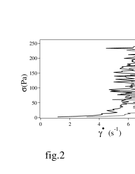
Figure 2: Shear thickening of a concentrated suspension of rough particles. The volume fraction is $\phi=0.37$. Stress is controlled in Couette geometry, and is increased from $0$ Pa to $255$ Pa, at a rate of $2.1$ Pa.s^-1 (continuous curve). Then, the stress is decreased down to zero with the same absolute rate (dashed curve). Shear thickening occurs for $\sigma\gtrsim 20$ Pa. A slight hysteresis is observed when the stress is decreased.

The mechanical properties of the sample and the occurring of jamming are illustrated by the rheological measurement reported in Fig. 2, in which the sample undergoes a ramp of stress. For small stresses, the shear rate increases smoothly with the stress; then, when the stress reaches a critical value, a transition occurs to a different regime, where the shear rate starts fluctuating around a fixed value. We will call this the shear jamming regime. If a decreasing ramp of stress is applied after the rising ramp, a slight hysteresis in the stress vs shear rate curve is observed.

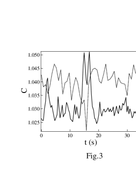
Figure 3: Fluctuations of the gradient (dotted line) and the contrast (solid line) under an applied stress of $50$ Pa. Low values of the gradient are associated to high values of the contrast.

Let us now apply a constant stress of $50$ Pa, above the jamming transition (Fig. 3). First, we observe that the shear rate is not stationary and exhibits huge fluctuations lootens . The observed contrast also fluctuates and its fluctuations are correlated to the shear rate fluctuations. When the sample is under shear, the faster and dominant movement of the particles is due to the flow. Assuming a linear shear rate, the typical timescale characterizing the scattered light intensity fluctuations is $\tau_{s}=\sqrt{10}/(\textbf{k}_{0}l^{*})1/\dot{\gamma}$, where $\textbf{k}_{0}=2\pi/\lambda$ is the laser beam wave vector, $\dot{\gamma}$ is the shear rate and $l^{*}$ is the photon transport mean free path in the medium wu . So, when the flow velocity decreases due to the shear rate fluctuations in the jamming regime, as the particles move slower, the contrast will be higher and viceversa.

Under high stress values, the dynamics of the particles under shear may even be slower than the dynamics at rest. In Fig. 4, we report an experiment in which a high stress value in the jamming regime, $\sigma=255$ Pa, is applied for $30$ s; then the application of stress is stopped. Before the shear, the contrast at rest is equal to $1.06$ and its relative fluctuations, calculated as the standard deviation of the signal divided by its average value diminished by $1$, are $4\%$. As soon as the stress is applied, the contrast drops to a smaller value $1.02$; then, the suspension jams and huge contrast fluctuations occur. Remarkably, these fluctuations lead to contrast values higher than the contrast value at rest before or after the stress application. This means that during the shear, the particles velocity becomes sometimes so small that $\tau_{s}$ is not the dominant timescale anymore, so another dynamical timescale of the system can be revealed. Moreover, the dynamics characterized by this sometimes emerging timescale is slower than the dynamics of the system at rest. The particles thus organized themselves under flow in such a way that their motion is slower than their free motion at rest. This is an important result as it is a direct evidence of the formation of a flow-induced structure whose dynamics is slower than the dynamics of the suspension’s at rest.

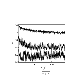
Figure 5: Contrast relaxation, soon after the application of a stress $\sigma=180$ Pa during $30$ s, for three different measurements performed under the same conditions. The measurements are highly non-reproducible. The overshoot of the contrast is not always observed, as exemplified by the bottom curve. The two other curves exhibit an overshoot, but its amplitude, its characteristic decorrelation time, the value of the baseline and the noise of the contrast signal vary with the measurement.

The dynamical properties of particles aggregates and their relaxation time are studied. We thus follow the evolution of the contrast after cessation of stress in the jamming regime. As soon as the stress application is stopped, we observe (Fig. 4) an overshoot of the contrast: just after stress cessation, the contrast value is much higher than the one at rest. It then slowly decreases to a constant value, which is not necessarily the same value it had before the shear. We observe that the contrast signal is very noisy. Let us moreover consider the noise amplitude along a relaxation curve (Fig. 4) : just after shear cessation ($60<t<80$ s), the amplitude of the fluctuations are smaller than after complete relaxation ($t>200$ s). The origin of the noise is discussed below. When the same measurement is repeated under the same conditions, the relaxation curve of the contrast may exhibit different properties (Fig. 5): its amplitude, its noise, the final value and the characteristic relaxation time vary with the measure; while sometimes the overshoot cannot be revealed either, as one of the three curves shows.

Though the contrast signal is very noisy, we investigated qualitatively the dependence of the relaxation contrast behavior on the applied stress value in the jamming regime. The evolution of the contrast after the shear stop has been studied for three different applied stress over the critical stress and for each stress a set of $8$ measurements under the same conditions has been performed. The sample is first sheared under a constant stress $\sigma\in\{100,\>180,\>255\}$ Pa for $30$ s, then stress application is ceased; the contrast value is recorded during the entire experiment. The curves which were not showing an overshoot have been dropped. We used the following criterium : we selected only the curves whose noise was smaller than the half-amplitude of the contrast decrease. The noise is measured as the standard deviation of the contrast when it reaches the final plateau value, i.e. when it is the highest. For the larger stress value, $\sigma=255$ Pa, none of the $8$ curves had to be dropped, for $\sigma=180$ Pa, $2$ of the set were dropped and $4$ for $\sigma=100$ Pa. In order to compare the relaxation times after the application of different stresses, we averaged the set of remaining contrast data for each stress value. As the contrast relaxation has an exponential behavior, we applied a logarithmic binning procedure to each averaged curve, in order to reduce noise at long time. Firstly, the points of the curve have been averaged in groups of ten, then they are further averaged in order to obtain a curve with $25$ points logarithmically spaced on the x-axis. The obtained curves of the averaged contrast evolution vs time after shear cessation for the three different stress values are plotted in Fig. 6, where, to be better compared, they have been normalized between $0$ and $1$. The curves are then fitted by a stretched exponential $C(t)=\exp(-t/\tau)^{\beta}$. The value of the $\tau$ parameter varies between $4$ s for the smaller stress and $29$ s for the bigger stress. As the value of the $\beta$ parameter does not remain constant, but varies between $0.5$ and $0.7$, the average relaxation time $\langle\tau\rangle$ is calculated :

$$\langle\tau\rangle=\int_{0}^{\infty}\textrm{e}^{-(t/\tau)^{\beta}}\>dt=\frac{\tau}{\beta}\>\>\Gamma(\frac{1}{\beta})$$ (1)

where $\Gamma$ is the Euler gamma function. The values of $\langle\tau\rangle$ are plotted as a function of the stress in Fig. 6 inset. Thus, at high stresses, where particles aggregates formation has been demonstrated, the contrast relaxation after shear cessation gets slower for increasing applied stress.

IV Discussion

These experiments thus lead to the following observations :

• the contrast fluctuates under shear, and may reach values higher than values at rest (Fig. 4),

• contrast relaxation curves after shear cessation exhibit huge noise amplitude (Fig. 5),

• the contrast relaxation time after shear cessation is an increasing function of the applied stress (Fig. 6).

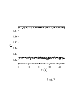
Figure 7: Contrast evolution for a system at rest, for different samples and different camera exposure times $T$. From top to bottom: silica spheres suspension for $T=191\>\>\mu s$, silica spheres suspension for $T=19.1\>\>ms$ and water solution of latex for $T=19.1\>\>ms$.

When put together, these observations give insight into the aggregates formation and disruption. But, first of all, let us discuss the origin of the high noise of the contrast signal. It is a consequence of both the properties of the system, and of our choice of the shutter duration $T=5.08$ ms, that maximizes the amplitude of the contrast relaxation after shear cessation. Indeed, the contrast is very noisy if compared to the amplitude of the relaxation (Fig. 5); this prevents us from making systematic measurements with an easy quantitative analysis of the results. This noise is not due to the setup, but is an intrinsic characteristic of the sample. This is shown in Fig. 7, where we plotted the contrast, measured at the camera exposure duration $T=19.1$ ms, for two samples at rest: the suspension of silica particles used in our work and a water solution of latex, taken as reference sample. The relative noise was calculated as the ratio between the standard deviation of the signal and the difference between its average value and $1$. We obtained a value of $0.011$ for the noise of the silica sample and of $0.0035$ for the one of the reference sample, which is then nearly an order of magnitude smaller. Besides, for a given sample, the noise of the contrast signal depends on the chosen $T$. The amplitude of the noise decreases when the exposure time $T$ decreases. Thus, the relative contrast noise for a silica suspension for $T=191\ \mu$s is smaller by a factor of $4$ than the noise for $T=19.1$ ms (Fig. 7). Nevertheless, as explained above, the value of $T$ was chosen in order to maximize the contrast variation during the entire experiment. For that value ($T=5.08$ ms), the amplitude of the noise is similar to that measured at $T=19.1$ ms.

IV.1 Aggregates formation under flow

When the suspension is submitted to a constant stress, high values of the contrast are associated to low values of the shear rate (Fig. 1). The contrast increase events are thus due to the formation of aggregates of macroscopic size that hinder the flow, and induce a drop of the shear rate. Moreover, the observed contrast under shear may reach higher values than contrast values at rest (Fig. 4). This observation has two consequences : dynamics of the particles inside the aggregates is slower than their dynamics at rest, and the volume occupied by particles belonging to aggregates is large enough so that position fluctuations of free particles inside the illuminated volume do not blur the speckle image.

IV.2 Spatial heterogeneities

In Fig. 4 we observed that, once the stress application is stopped, the contrast plateau value after the relaxation is different from the contrast value at rest before stress application. Besides, Fig. 5 shows that this plateau value varies at each measurement. As the ensemble of measurements presented in Fig. 5 are taken with the same sample under the same conditions, it can be considered as a sampling in which a different region of the system after shear cessation is observed during each measurement. The presence of spatial heterogeneities in the system, consisting in slower and faster regions, due to the very high concentration of the suspension may be responsible for this lack of reproducibility. Indeed, if the heterogeneities length-scale is of the order of the illuminated volume size, the non reproducibility of the contrast value at rest may be easily explained. After each shear cessation, the illuminated region would be characterized by a different local concentration and then a different dynamical timescale inducing different contrast values. Fig. 5 thus gives us some qualitative insight into the aggregates size. The amplitude of the relaxation of the contrast depends on the relative size of the aggregates in the illuminated volume. It has been shown by numerical simulations loan , that the presence of aggregates spanning the entire system is characteristic of the jamming regime. The varying amplitude of the contrast relaxation for different measurements implies that the aggregates size is comparable to the illuminated region, thus confirming the mechanical results. Unfortunately, a study of the aggregate size distribution is not possible, due to the fact that the illuminated region, representing a fraction of the entire cell gap, may contain only a part of an aggregate. Moreover, for the lowest studied values of the applied stress, the contrast doesn’t always exhibit an overshoot after the application of shear. There must thus exist some regions, at least as large as the illuminated volume, without any of the macroscopic aggregates responsible for the jamming. This gives a lower limit of the average distance among the aggregates, which must be at least of the maximum linear size of the illuminated region, i.e. $6$ mm.

IV.3 Contrast fluctuations

The existence of such heterogeneities allows us to understand the observed large fluctuations of the contrast and the evolution of their amplitude during relaxation. The decorrelation time $\tau_{c}$ for $g_{1}$, characterizing the dynamics of the system, will have a certain distribution $\Delta\tau_{c}$. Remembering that the contrast can be considered as a function of $g_{1}$ durian , a large decorrelation time distribution will induce large fluctuations in the contrast signal. Moreover, the amplitude of this fluctuations will also depend on the value of $T$ relatively to the decorrelation time. Thus, let us assume that the system is characterized by a decorrelation time belonging to $[\tau_{0}-\Delta\tau_{0},\tau_{0}+\Delta\tau_{0}]$ with $\Delta\tau_{0}=\tau_{0}/10$ soon after the shear stop, and by a characteristic time $\tau_{1}>\tau_{0}$ with distribution $\Delta\tau_{1}=\tau_{1}/10$ when it has relaxed to equilibrium. In order to obtain the maximum value of the contrast, we chose $T=\sqrt{\tau_{0}\tau_{1}}$, as detailed in Fig. 1. Choosing for instance $\tau_{0}=1$ and $\tau_{1}=100$, the amplitude of the contrast fluctuations may be computed. One gets that fluctuations for dynamics faster than the exposure time are $\sim 15$ times larger than fluctuations for slower dynamics. This computation agrees with the contrast fluctuations observed in Fig. 4, where the contrast noise soon after the shear cessation ($60<t<80$ s), i.e for the slowest dynamics, is smaller than the noise after the contrast relaxation ($t>200$ s), when the dynamics is the fastest.

IV.4 Stress dependency

Finally, from the study of the contrast relaxation at different stresses, we observed that, the higher the stress, the more frequently the contrast overshoot shows up. Thus, the volume fraction of macroscopic aggregates in the system increases with the applied stress, leading to an increase of the probability to observe one of them when stress is ceased. Nevertheless, we did not observe any dependency of the amplitude of the contrast relaxation after shear cessation on the applied stress. As long as the aggregates are smaller than the illuminated volume, this amplitude is a measure of the volume fraction of the aggregates inside the illuminated volume. As a consequence, the observed increase of the aggregates volume fraction would not be due to an increase of the aggregates size, but of the aggregates number. Nevertheless, direct confocal microscopy observations suggest that the jammed regions may be larger than the diameter of our beam ($6$ mm) lootens2 . Thus, an increase of the aggregates size as a function of the applied stress cannot be ruled out.
Two phenomena may thus be responsible for our last result. We observed that, on average, for larger applied stresses, the relaxation time of the aggregates is longer (Fig. 6 inset). On one hand, an increase of the size of the aggregates, as the applied stress value is increased, may occur. On the other hand, colloids organization and volume fraction inside the aggregates may depend on the applied stress. Thus, numerical simulations of concentrated colloids under shear melrose1 show that the distance between neighboring particles inside the aggregates decreases when the applied stress increases. If similar behavior occurs in our system, as also indicated by confocal microscopy observations lootens2 , the volume fraction of particles inside aggregates increases with the applied stress, which favors a slowing down of aggregates disruption.

V Conclusion

We investigated the aggregates relaxation after shearing a suspension of concentrated silica particles in the jamming regime. Under flow, the observed peaks in the contrast showed that aggregates form. The dynamics of the particles under flow may even be slower than their dynamics at rest. When the shear is stopped, the contrast relaxes back to a lower value, giving evidence of the reversibility of the aggregates. The suspension under flow and just after flow cessation is extremely heterogeneous. The characteristic size of the heterogeneities is of the order of magnitude of the illuminated volume in the SVS experiment, i.e. of the order of the cell thickness. The contrast signal thus exhibits huge fluctuations and measurements are not easily reproducible, as they depend on the particular volume sampled during each experiment. Nevertheless, by carefully averaging the contrast relaxation over several measurements, it was observed that the higher the applied stress, the slower the aggregates relaxation. Several phenomena may be responsible for this behavior : an increase of the aggregates size and volume fraction, as also indicated by the increase of the occurrence of contrast overshoot with the applied stress, or a decrease of intercolloidal distances inside aggregates, as suggested by numerical simulations melrose1 . Further experiments should allow to choose among the interpretations proposed.

The authors wish to thank R. Di Leonardo and G. Ruocco for fruitful discussions.

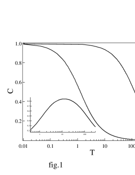
Figure 1: Evolution of the contrast with the camera exposure duration $T$. The dynamics of the electric field correlation function $g_{1}$ is assumed to be characterized by a single relaxation time, $\tau_{c}$. Continuous curve : $\tau_{c}=\tau_{c}^{0}=100$. Dashed curve : $\tau_{c}=\tau_{c}^{1}=1$. Inset : difference between the two contrast curves, $C_{\tau_{c}^{0}}(T)-C_{\tau_{c}^{1}}(T)$ as a function of $T$. The maximum difference is obtained for a $T$ value approximately equal to the geometric average of $\tau_{c}^{0}$ and $\tau_{c}^{1}$, $\sqrt{\tau_{c}^{0}\tau_{c}^{1}}$

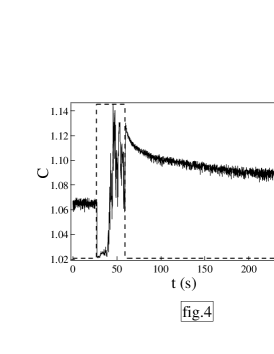
Figure 4: Contrast behavior before, during and after the application of a stress $\sigma=255$ Pa during $30$ s. The stress history is plotted in dashed line. During the stress application, strong contrast fluctuations are observed. After the shear cessation, the contrast exhibits an overshoot and then relaxes to a constant value.

Figure 6: Normalized and averaged contrast relaxations curves after the application of a constant stress $\sigma$ during $30$ s. Three values of the applied stress are studied. $\blacksquare$ :$\sigma=100$ Pa, $\blacktriangle$ :$\sigma=180$ Pa and $\blacklozenge$ :$\sigma=255$ Pa. Each curve is fitted with a stretched exponential form : $C(t)=e^{-(\frac{t}{\tau})^{\beta}}$. Inset : average relaxation time, $\bar{\tau}=\int_{0}^{\infty}exp[-(t/\tau)^{\beta}]\>dt=\tau/\beta\>\>\Gamma(1/\beta)$ as a function of the applied stress.

References

- (1) D. Lootens, H. Van Damme, P. Hebraud, Phys. Rev. Lett. 90, 178301 (2003).
- (2) B.J. Maranzano, N.J. Wagner, J. Rheol. 45, 1205 (2001).
- (3) R.S. Farr, J.R. Melrose, R.C. Ball, Phys. Rev. E 55, 7203 (1997).
- (4) P. Raiskinmaki, J.A. Astrom, M. Kataja, M. Latva-Kokko, A. Koponen, A. Jasberg, A. Shakib-Manesh, J. Timonen, Phys. Rev. E 68, 061403 (2003).
- (5) J. Bergenholtz, J.F. Brady, M. Vivic, J. Fluid Mech. 456, 239 (2002).
- (6) I.E. Zarraga, D.A. Hill, D.T. Leighton, Jr., J. Rheol. 44, 2, 185-200, 2000.
- (7) J. Bender, N.J. Wagner, J. Rheol. 40, 899 (1996).
- (8) O.J. O’Loan, M.R. Evans, M.E. Cates, Physica A 258, 109 (1998).
- (9) R.C. Ball, J.R. Melrose, Adv. Colloid Interface Sci. 59, 19 (1995).
- (10) H.M.Laun, R. Bung, S. Hess, W. Loose, O. Hesse, K. Hahn, E. Hadicke, R. Hingmann, F. Schmidt, P. Lindner, J. Rheol. 36, 743 (1992).
- (11) H. Watanabe, M-L. Yao, K. Osaki, T. Shikata, H. Niwa, Y. Morishima, N. P. Balsara, H. Wang, Rheol. Acta 37, 1 (1998).
- (12) V.G. Kolli, E.J. Pollauf, F. Gadala-Maria, J. Rheol. 46, 321 (2002).
- (13) M.D. Haw, Phys. Rev. Lett. 92, 185506 (2004).
- (14) P. Varadan, M.J. Solomon, J. Rheol. 47, 943 (2003).
- (15) P.K. Dixon, D.J. Durian, Phys. Rev. Lett. 90, 184302 (2003).
- (16) D. Lootens, H. van Damme, Y. Hémar, P. Hébraud, Phys. Rev. Lett., to be published.
- (17) D.J. Pine, D.A. Weitz, P.M.Chaikin, E. Herbolzheimer, Phys. Rev. Lett. 60, 1134 (1988).
- (18) L. Cipelletti, D.A. Weitz, Rev. Sci. Instrum. 70, 3214 (1999).
- (19) W. Stober and A. Fink, J. Colloid Interface Science. 26, 62 (1968).
- (20) R.K. Iler, The Chemistry of Silica, John Wiley, 1979.
- (21) R.L. Hoffman, J. Rheol. 42, 111 (1998).
- (22) D. Lootens, Ciments et suspensions concentr es mod les. coulement, encombrement et floculation, PhD thesis (2004).
- (23) R. Bandyopadhyay, A.S. Gittings, S.S. Suh, P.K. Dixon, D.J. Durian, preprint cond-mat/0506081, 2005.
- (24) B.J. Berne and R. Pecora, Dynamic Light Scattering, Dover Publications (1976).
- (25) X.L. Wu, D.L. Pine, P.M. Chaikin, J.S. Huang, D.A. Weitz, J. Opt. Soc. Am. B 7, 15 (1990).