A general geometric growth model for pseudofractal scale-free web

Abstract

We propose a general geometric growth model for pseudofractal scale-free web, which is controlled by two tunable parameters. We derive exactly the main characteristics of the networks: degree distribution, second moment of degree distribution, degree correlations, distribution of clustering coefficient, as well as the diameter, which are partially determined by the parameters. Analytical results show that the resulting networks are disassortative and follow power-law degree distributions, with a more general degree exponent tuned from 2 to $1+\frac{\ln 3}{\ln 2}$; the clustering coefficient of each individual node is inversely proportional to its degree and the average clustering coefficient of all nodes approaches to a large nonzero value in the infinite network order; the diameter grows logarithmically with the number of network nodes. All these reveal that the networks described by our model have small-world effect and scale-free topology.

1 Introduction

Since the pioneering papers by Watts and Strogatz on small-world networks [1] and Barabási and Albert on scale-free networks [2], complex networks, which describe many systems in nature and society, have become an area of tremendous recent interest [3, 4, 5, 6, 7]. In the last few years, modeling real-life systems has attracted an exceptional amount of attention within the physics community. While a lot of models have been proposed, most of them are stochastic [3, 4, 5, 6, 7]. However, because of their advantages, deterministic networks have also received much attention [8, 9, 10, 11, 12, 13, 14, 15, 16, 17, 18, 19, 20, 21, 22, 23, 24, 25, 26, 27, 28, 29, 30, 31]. First, the method of generating deterministic networks makes it easier to gain a visual understanding of how networks are shaped, and how do different nodes relate to each other [8]; moreover, deterministic networks allow to compute analytically their properties: degree distribution, clustering coefficient, average path length, diameter, betweenness, modularity and adjacency matrix whose eigenvalue spectrum characterizes the topology [8, 9, 10, 11, 12, 13, 14, 15, 16, 17, 18, 19, 20, 21, 22, 23, 24, 25, 26, 27, 28, 29, 30, 31].

The first model for deterministic scale-free networks was proposed by Barabási et al. in Ref. [8] and was intensively studied in Ref. [9]. Another elegant model, called pseudofractal scale-free web (PSW) [10], was introduced by Dorogovtsev, Goltsev, and Mendes, and was extended by Comellas et al. in Ref. [11]. Based on a similar idea of PSW, Jung et al. presented a class of recursive trees [12]. Additionally, in order to discuss modularity, Ravasz et al. proposed a hierarchical network model [13, 14], the exact scaling properties and extensive study of which were reported in Refs. [15] and [16], respectively. Recently, In relation to the problem of Apollonian space-filing packing, Andrade et al. introduced Apollonian networks [17] which were also proposed by Doye and Massen in Ref. [18] and have been intensively investigated [22, 23, 32, 33, 34, 35, 36]. In addition to the above models, deterministic networks can be created by various techniques: modification of some regular graphs [24], addition and product of graphs [25], edge iterations [26, 27] and other mathematical methods as in Refs. [28, 29, 30, 31].

As mentioned by Barabási et al., it would be of major theoretical interest to construct deterministic models that lead to scale-free networks [8]. Here we do an extensive study on pseudofractal scale-free web [10]. The PSW can be considered as a process of edge multiplication. In fact, a clique (edge is a special case of it) can also reproduce new cliques and the number of the new reproduction may be different at a time. Motivated by this, in a simple recursive way we propose a general model for PSW by including two parameters, with PSW as a particular case of the present model. The deterministic construction of our model enables one to obtain the analytic solutions for its structure properties. By adjusting the parameters, we can obtain a variety of scale-free networks.

2 The general geometric growth model

Before introducing our model we give the following definitions on a graph (network). The term size refers to the number of edges in a graph. The number of nodes in a graph is called its order. When two nodes of a graph are connected by an edge, these nodes are said to be adjacent, and the edge is said to join them. A complete graph is a graph in which all nodes are adjacent to one another. Thus, in a complete graph, every possible edge is present. The complete graph with $q$ nodes is denoted as $K_{q}$ (also referred in the literature as $q$-clique). Two graphs are isomorphic when the nodes of one can be relabeled to match the nodes of the other in a way that preserves adjacency. So all $q$-cliques are isomorphic to one another.

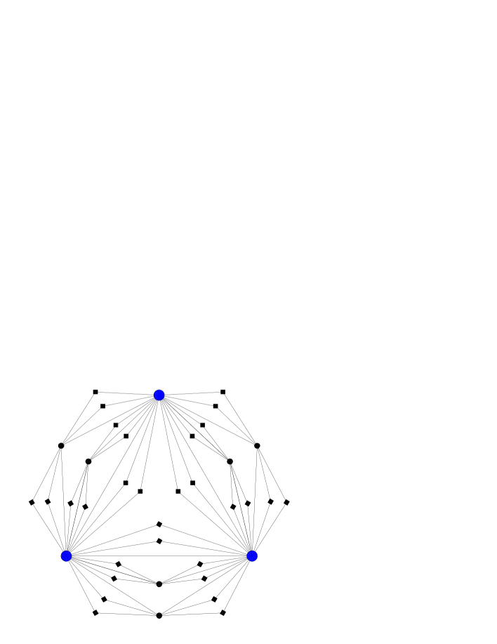
Figure 1: Scheme of the growth of the deterministic network for the case of $m=2$ and $q=2$. Only the first three steps are shown.

The network is constructed in a recursive way. We denote the network after $t$ steps by $R(q,t)$, $q\geq 2,t\geq 0$ (see Fig. 1). Then the network at step $t$ is constructed as follows: For $t=0$, $R(q,0)$ is a complete graph $K_{q+1}$ (or $(q+1)$-clique) consist of $q+1$ $q$-cliques), and $R(q,0)$ has $q+1$ nodes and $q(q+1)/2$ edges. For $t\geq 1$, $R(q,t)$ is obtained from $R(q,t-1)$ by adding $m$ new nodes for each of its existing subgraphs isomorphic to a $q$-clique, and each new node is connected to all the nodes of this subgraph. In the special case $m=1$ and $q=2$, it is reduced to the pseudofractal scale-free web described in Ref. [10]. In the limiting case of $m=1$, we obtain the same networks as in Ref. [11]. However, our family is richer as $m$ can take any natural value.

There is an interpretation called ‘aggregation’ [37] for our model. As an example, here we only explain them for the case of $m=1$ and $q=2$. Figure 2 illustrates the growing process for this particular case, which may be accounted for as an ‘aggregation’ process described in detail as follows. First, three of the initial triangle ($t=0$) are assembled to form a new unit ($t=1$). Then we assemble three of these units at the hubs (the nodes with highest degree) in precise analogy with the step leading from $t=0$ to $t=1$ to form a new cell ($t=2$) (see Fig. 3). This process can be iterated an arbitrary number of times. Moreover, an alternative explanation of our model which is often useful is that of ‘miniaturization’ (see Ref. [37]).

Figure 2: Growth process of pseudofractal scale-free web (i.e. the case of $m=1$ and $q=2$), exhibiting the first three steps.

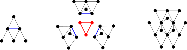
Figure 3: Aggregation process from $R(2,1)$ to $R(2,2)$, which is obtained by adjoining of three copies of $R(2,1)$ at the hubs.

3 Structural properties

Below we will find that the tunable parameters $m$ and $q$ control some relevant characteristics of the network $R(q,t)$. Because $q=2$ is a particular case, for conveniences, we treat $q=2$ and $q\geq 3$ separately.

3.1 Limiting case of $q=2$

Order and size. In the case of $q=2$, we denote $R(q,t)$ by $\mathcal{G}(t)$. Let us consider the total number of nodes $N_{t}$ and total number of edges $E_{t}$ in $\mathcal{G}(t)$. Denote $n_{v}(t)$ as the number of nodes created at step $t$. Note that the addition of each new node leads to two new edges. By construction, for $t\geq 1$, we have

$$n_{v}(t)=mE_{t-1}$$ (1)

and

$$E_{t}=E_{t-1}+2n_{v}(t).$$ (2)

Considering the initial condition $n_{v}(0)=3$ and $E_{0}=3$, it follows that

$$n_{v}(t)=3m\,(2m+1)^{t-1}\quad\ \hbox{and}\quad\ E_{t}=3\,(2m+1)^{t}.$$ (3)

Then the number of nodes increases with time exponentially and the total number of nodes present at step $t$ is

$$N_{t}=\sum_{t_{i}=0}^{t}n_{v}(t_{i})=\frac{3\,(2m+1)^{t}+3}{2}.$$ (4)

Thus for large $t$, The average degree $\overline{k}_{t}=\frac{2E_{t}}{N_{t}}$ is approximately $4$.

Degree distribution. Let $k_{i}(t)$ be the degree of node $i$ at step $t$. Then by construction, it is not difficult to find following relation:

$$k_{i}(t)=(m+1)k_{i}(t-1),$$ (5)

which expresses a preference attachment [2]. If node $i$ is added to the network at step $t_{i}$, $k_{i}(t_{i})=2$ and hence

$$k_{i}(t)=2\,(m+1)^{t-t_{i}}.$$ (6)

Therefore, the degree spectrum of the network is discrete. It follows that the degree distribution is given by

$$P(k)=\left\{\begin{array}[]{lc}{\displaystyle{n_{v}(0)\over N_{t}}={2\over(2m+1)^{t}+1}}&\ \hbox{for}\ t_{i}=0\\ {\displaystyle{n_{v}(t_{i})\over N_{t}}={2m\,(2m+1)^{t_{i}-1}\over(2m+1)^{t}+1}}&\ \hbox{for}\ t_{i}\geq 1\\ 0&\ \hbox{otherwise}\end{array}\right.$$ (7)

and that the cumulative degree distribution [6, 10] is

$$P_{\rm cum}(k)=\sum_{\rho\leq t_{i}}\frac{n_{v}(\rho)}{N_{t}}={(2m+1)^{t_{i}}+1\over(2m+1)^{t}+1}.$$ (8)

Substituting for $t_{i}$ in this expression using $t_{i}=t-\frac{\ln(k/2)}{\ln(m+1)}$ gives

$$P_{\rm cum}(k) = {(2m+1)^{t}\left({k/2}\right)^{-\frac{\ln(2m+1)}{\ln(m+1)}}+1\over(2m+1)^{t}+1}$$ (9)

$$\approx \left({k\over 2}\right)^{\textstyle-{\ln(2m+1)\over\ln(m+1)}}\qquad\hbox{for large $t$}.$$

So the degree distribution follows the power law with the exponent $\gamma=1+{\frac{\ln(2m+1)}{\ln(m+1)}}$. For the particular case of $m=1$, Eq. (9) recovers the result previously obtained in Ref. [10].

Second moment of degree distribution. Let us calculate the second moment of degree distribution $\langle k^{2}\rangle$. It is defined by

$$\langle k^{2}\rangle=\frac{1}{N_{t}}\sum_{t_{i}=0}^{t}n_{v}(t_{i})\left[k(t_{i},t)\right]^{2},$$ (10)

where $k(t_{i},t)$ is the degree of a node at step $t$, which was generated at step $t_{i}$. This quality expresses the average of degree square over all nodes in the network. It has large impact on the dynamics of spreading [38, 39] and the onset of percolation transitions [40, 41] taking place in networks. when $\langle k^{2}\rangle$ is diverging, the networks allow the onset of large epidemics whatever the spreading rate of the infection [38, 39], at the same time the networks are extremely robust to random damages, in other words, the percolation transition is absent [40, 41].

substituting Eqs. (3), (4) and (6) into Eq. (10), we derive

$$\langle k^{2}\rangle = \frac{8}{1+\frac{1}{(2m+1)^{t}}}\left[\left(\frac{1}{m}+1\right)\left(\frac{(m+1)^{2}}{2m+1}\right)^{t}-\frac{1}{m}\right]$$ (11)

$$\approx \frac{8\,(m+1)^{2t+1}}{m(2m+1)}\rightarrow\infty\qquad\hbox{for large $t$.}$$

In this way, second moment of degree distribution $\langle k^{2}\rangle$ has been calculated explicitly, and result shows that it diverges as an exponential law. So the networks are resilient to random damage and are simultaneously sensitive to the spread of infections.

Degree correlations. As the field has progressed, degree correlation [42, 43, 44, 45, 46] has been the subject of particular interest, because it can give rise to some interesting network structure effects. An interesting quantity related to degree correlations is the average degree of the nearest neighbors for nodes with degree $k$, denoted as $k_{\rm nn}(k)$ [43, 44]. When $k_{\rm nn}(k)$ increases with $k$, it means that nodes have a tendency to connect to nodes with a similar or larger degree. In this case the network is defined as assortative [45, 46]. In contrast, if $k_{\rm nn}(k)$ is decreasing with $k$, which implies that nodes of large degree are likely to have near neighbors with small degree, then the network is said to be disassortative. If correlations are absent, $k_{\rm nn}(k)=const$.

We can exactly calculate $k_{\rm nn}$ for the networks using Eq. (6) to work out how many links are made at a particular step to nodes with a particular degree. Except for three initial nodes generated at step 0, no nodes born in the same step, which have the same degree, will be linked to each other. All links to nodes with larger degree are made at the creation step, and then links to nodes with smaller degree are made at each subsequent steps. This results in the expression

$$k_{\rm nn}(k)={1\over n_{v}(t_{i})k(t_{i},t)}\Bigg{(}\sum_{t^{\prime}_{i}=0}^{t^{\prime}_{i}=t_{i}-1}m\cdot n_{v}(t^{\prime}_{i})k(t^{\prime}_{i},t_{i}-1)k(t^{\prime}_{i},t)+$$

$$\qquad\qquad\qquad\qquad\qquad\sum_{t^{\prime}_{i}=t_{i}+1}^{t^{\prime}_{i}=t}m\cdot n_{v}(t_{i})k(t_{i},t^{\prime}_{i}-1)k(t^{\prime}_{i},t)\Bigg{)}$$ (12)

for $k=2\,(m+1)^{t-t_{i}}$. Here the first sum on the right-hand side accounts for the links made to nodes with larger degree (i.e. $t^{\prime}_{i}<t_{i}$) when the node was generated at $t_{i}$. The second sum describes the links made to the current smallest degree nodes at each step $t^{\prime}_{i}>t_{i}$.

Substituting Eqs. (3) and (6) into Eq. (3.1), after some algebraic manipulations, Eq. (3.1) is simplified to

$$k_{\rm nn}(k)=\frac{2(2m+1)}{m}\,\left[\frac{(m+1)^{2}}{2m+1}\right]^{t_{i}}-\frac{2(m+1)}{m}+\frac{2m}{m+1}\,(t-t_{i}).$$ (13)

Thus after the initial step $k_{\rm nn}$ grows linearly with time.

Writing Eq. (13) in terms of $k$, it is straightforward to obtain

$$k_{\rm nn}(k)=\frac{2(2m+1)}{m}\,\left[\frac{(m+1)^{2}}{2m+1}\right]^{t}\,\left(\frac{k}{2}\right)^{-\frac{\ln\left[\frac{(m+1)^{2}}{2m+1}\right]}{\ln(m+1)}}$$

$$\qquad\qquad\qquad\qquad-\frac{2(m+1)}{m}+\frac{2m}{m+1}\,\frac{\ln(\frac{k}{2})}{\ln(m+1)}.$$ (14)

Therefore, $k_{\rm nn}(k)$ is approximately a power law function of $k$ with negative exponent, which shows that the networks are disassortative. Note that $k_{\rm nn}(k)$ of the Internet exhibit a similar power-law dependence on the degree $k_{\rm nn}(k)\sim k^{-\omega}$, with $\omega=0.5$ [43].

Clustering coefficient. The clustering coefficient defines a measure of the level of cohesiveness around any given node. By definition, the clustering coefficient [1] $C_{i}$ of node $i$ is the ratio between the number of edges $e_{i}$ that actually exist among the $k_{i}$ neighbors of node $i$ and its maximum possible value, $k_{i}(k_{i}-1)/2$, i.e., $C_{i}=2e_{i}/k_{i}(k_{i}-1)$. The clustering coefficient of the whole network is the average of all individual $C_{i}^{\prime}s$. Next we will compute the clustering coefficient of every node and their average value.

Obviously, when a new node $i$ joins the network, its degree $k_{i}$ and $e_{i}$ is $2$ and $1$, respectively. Each subsequent addition of a link to that node increases both $k_{i}$ and $e_{i}$ by one. Thus, $e_{i}$ equals to $k_{i}-1$ for all nodes at all steps. So one can see that, there is a one-to-one correspondence between the degree of a node and its clustering. For a node with degree $k$, the exact expression for its clustering coefficient is $2/k$. Therefore, the clustering coefficient spectrum of nodes is discrete. Using this discreteness, it is convenient to work with the cumulative distribution of clustering coefficient [10] as

$$W_{\rm cum}(C)=\frac{1}{N_{t}}\sum_{t_{j}\geq t_{i}}\frac{2n_{v}(t_{j})}{k(t_{j},t)}\sim C^{{\frac{\ln(2m+1)}{\ln(m+1)}}}=C^{\gamma-1}.$$ (15)

It is worth noting that for the special case of $m=1$, this result has been obtained previously [10].

The clustering coefficient of the whole network at arbitrary step $t$ can be easily computed,

$$\overline{C}_{t}=\frac{1}{N_{t}}\sum_{r=0}^{t}\frac{2\,n_{v}(r)}{k(r,t)}=\frac{2m+2}{2m+3}\,\frac{(m+1)^{t}(2m+1)^{t}+\frac{m+2}{m+1}}{(m+1)^{t}[(2m+1)^{t}+1]}.$$ (16)

In the infinite network size limit ($t\rightarrow\infty$), $\overline{C}=(2m+2)/(2m+3)$. Thus the clustering $\overline{C}$ is high and increases with $m$. Moreover, similarly to the degree exponent $\gamma$, $\overline{C}$ is tunable by choosing the right value of parameter $m$: in particular, $\overline{C}$ ranges from $4/5$ (in the special case of $m=1$ [10]) to limit of 1 when $m$ becomes very large.

Diameter. The diameter of a network is defined as the maximum of the shortest distances between all pairs of nodes, which characterizes the longest communication delay in the network. Small diameter is consistent with the concept of small-world and it is easy to compute for our networks. Below we give the precise analytical computation of diameter of $\mathcal{G}(t)$ denoted by $Diam(\mathcal{G}(t))$.

It is easy to see that at step $t=0$ (resp. $t=1$), the diameter is equal to 1 (resp. 2). At each step $t\geq 2$, one can easily see that the diameter always lies between a pair of nodes that have just been created at this step. In order to simplify the analysis, we first note that it is unnecessary to look at all the nodes in the networks in order to find the diameter. In other words, some nodes added at a given step can be ignored, because they do not increase the diameter from the previous step. These nodes are those that connect to edges that already existed before step $t-1$. Indeed, for these nodes we know that a similar construction has been done in previous steps, so we can ignore them for the computation of the diameter. Let us call “outer” nodes the nodes which are connected to a edge that did not exist at previous steps. Clearly, at each step, the diameter depends on the distances between outer nodes.

At any step $t\geq 2$, we note that an outer node cannot be connected with two or more nodes that were created during the same step $t^{{}^{\prime}}\geq t-1$. Indeed, we know that from step $2$, no outer node is connected to two nodes of the initial triangle $\mathcal{G}(0)$. Thus, for any step $t\geq 2$, any outer node is connected with nodes that appeared at pairwise different steps. Now consider two outer nodes created at step $t\geq 2$, say $v_{t}$ and $w_{t}$. Then $v_{t}$ is connected to two nodes, and one of them must have been created before or during step $t-2$. We repeat this argument, and we end up with two cases: (1) $t=2m$ is even. Then, if we make $m$ “jumps”, from $v_{t}$ we reach the initial triangle $\mathcal{G}(0)$, in which we can reach any $w_{t}$ by using an edge of $\mathcal{G}(0)$ and making $m$ jumps to $w_{t}$ in a similar way. Thus $Diam(\mathcal{G}(2m))\leq 2m+1$. (2) $t=2m+1$ is odd. In this case we can stop after $m$ jumps at $\mathcal{G}(1)$, for which we know that the diameter is 2, and make $m$ jumps in a similar way to reach $w_{t}$. Thus $Diam(\mathcal{G}(2m+1))\leq 2(m+1)$. It is easily seen that the bound can be reached by pairs of outer nodes created at step $t$. More precisely, those two nodes $v_{t}$ and $w_{t}$ share the property that they are connected to two nodes that appeared respectively at steps $t-1$, $t-2$.

Hence, formally, $Diam(\mathcal{G}(t))=t+1$ for any $t\geq 0$. Note that $N_{t}\sim(2m+1)^{t}$, thus the diameter is small and scales logarithmically with the number of network nodes.

3.2 Case of $q\geq 3$

In these cases, the analysis is a little difficult than those of the last subsection. An alternative approach has to be adopted, although it may also holds true for the first case in some situations. The method of the last subsection is relatively easy to generalize to these cases, and below we will address it, focusing on order, size, degree distribution, clustering coefficient and diameter.

Order and size. Let $n_{v}(t)$, $n_{e}(t)$ be the number of nodes and edges created at step $t$, respectively. Denote $K_{q,t}$ as the total number of $q$-cliques in the whole network at step $t$. Note that the addition of each new node leads to $q$ new $q$-cliques and $q$ new edges. By construction, we have $n_{e}(t)=qn_{v}(t)$, $n_{v}(t)=mK_{q,t-1}$ and $K_{q,t}=K_{q,t-1}+qn_{v}(t)$. Thus one can easily obtain $K_{q,t}=(mq+1)K_{q,t-1}=(q+1)(mq+1)^{t}$ ($t\geq 0$), $n_{v}(t)=m(q+1)(mq+1)^{t-1}$ ($t>0$) and $n_{e}(t)=mq(q+1)(mq+1)^{t-1}$ ($t>0$). From above results, we can easily compute the order and size of the networks. The total number of nodes $N_{t}$ and edges $E_{t}$ present at step $t$ is

$$N_{t}=\sum_{t_{i}=0}^{t}n_{v}(t_{i})=\frac{(q+1)[(mq+1)^{t}+q-1]}{q}$$ (17)

and

$$E_{t}=\sum_{t_{i}=0}^{t}n_{e}(t_{i})=(q+1)(mq+1)^{t}+\frac{(q+1)(q-2)}{2},$$ (18)

respectively. For infinite $t$, the average degree $\overline{k}_{t}=\frac{2E_{t}}{N_{t}}$ is approximately $2q$.

Degree distribution. When a new node $i$ is added to the graph at step $t_{i}$, it has degree $q$ and forms $q$ new $q$-cliques. Let $n_{q}(i,t)$ be the total number of $q$-cliques at step $t$ that will created new nodes connected to the node $i$ at step $t+1$. So at step $t_{i}$, $n_{q}(i,t_{i})=q$. By construction, we can see that in the subsequent steps each new neighbor of $i$ generates $q-1$ new $q$-cliques with $i$ as one node of them. Let $k_{i}(t)$ be the degree of $i$ at step $t$. It is not difficult to find following relations for $t>t_{i}+1$:

$$\Delta k_{i}(t)=k_{i}(t)-k_{i}(t-1)=mn_{q}(i,t-1)$$ (19)

and

$$n_{q}(i,t)=n_{q}(i,t-1)+(q-1)\Delta k_{i}(t).$$ (20)

From the above two equations, we can derive $n_{q}(i,t)=[m(q-1)+1]n_{q}(i,t-1)$. Considering $n_{q}(i,t_{i})=q$, we obtain $n_{q}(i,t)=q[m(q-1)+1]^{t-t_{i}}$ and $\Delta k_{i}(t)=mq[m(q-1)+1]^{t-t_{i}-1}$. Then the degree $k_{i}(t)$ of node $i$ at time $t$ is

$$k_{i}(t) = k_{i}(t_{i})+\sum_{t_{h}=t_{i}+1}^{t}{\Delta k_{i}(t_{h})}$$ (21)

$$= \frac{q[m(q-1)+1]^{t-t_{i}}+q^{2}-2q}{q-1}.$$

Since the degree of each node has been obtained explicitly as in Eq. (21), we can get the degree distribution via its cumulative distribution [6, 10], i.e. $P_{cum}(k)\equiv\sum_{k^{\prime}\geq k}N(k^{\prime},t)/N_{t}\sim k^{1-\gamma}$, where $N(k^{\prime},t)$ denotes the number of nodes with degree $k^{\prime}$. The analytic computation details are given as follows. For a degree $k$

$$k=\frac{q[m(q-1)+1]^{t-j}+q^{2}-2q}{q-1},$$ (22)

there are $n_{v}(j)=m(q+1)(qm+1)^{j-1}$ nodes with this exact degree, all of which were born at step $j$. All nodes with birth time at $j$ or earlier have this and a higher degree. So we have

$$\sum_{k^{\prime}\geq k}N(k^{\prime},t)=\sum_{s=0}^{j}n_{v}(s)=\frac{(q+1)[(mq+1)^{j}+q-1]}{q}.\\$$

As the total number of nodes at step $t$ is given in Eq. (17), we have

$$\left[\frac{q[m(q-1)+1]^{t-j}+q^{2}-2q}{q-1}\right]^{1-\gamma}\\ =\frac{\frac{(q+1)[(mq+1)^{j}+q-1]}{q}}{\frac{(q+1)[(mq+1)^{t}+q-1]}{q}}.\\$$

Therefore, for large $t$ we obtain

$$\left[[m(q-1)+1]^{t-j}\right]^{1-\gamma}=(mq+1)^{j-t}$$ (23)

and

$$\gamma\approx 1+\frac{\ln(mq+1)}{\ln[m(q-1)+1]}.$$ (24)

For the special case $m=1$, Eq. (24) recovers the results previously reported in Ref. [11].

Clustering coefficient. The analytical expression for clustering coefficient $C(k)$ of the individual node with degree $k$ can be derived exactly. When a node is created it is connected to all the nodes of a $q$-clique whose nodes are completely interconnected. Its degree and clustering coefficient are $q$ and 1, respectively. In the following steps, if its degree increases one by a newly created node connecting to it, then there must be $q-1$ existing neighbors of it attaching to the new node at the same time. Thus for a node of degree $k$, we have

$$C(k)={{{q(q-1)\over 2}+(q-1)(k-q)}\over{k(k-1)\over 2}}=\frac{2(q-1)(k-\frac{q}{2})}{k(k-1)},$$ (25)

which depends on degree $k$ and $q$. For $k\gg q$, the $C(k)$ is inversely proportional to node degree. The scaling $C(k)\sim k^{-1}$ has been found for some network models [4, 5, 6, 7], and has also observed in several real-life networks [14].

Using Eq. (25), we can obtain the clustering $\overline{C}_{t}$ of the networks at step $t$:

$$\overline{C}_{t}=\frac{1}{N_{t}}\sum_{r=0}^{t}\frac{2(q-1)(D_{r}-\frac{q}{2})n_{v}(r)}{D_{r}(D_{r}-1)},$$ (26)

where the sum is the total of clustering coefficient for all nodes and $D_{r}=\frac{q[m(q-1)+1]^{t-r}+q^{2}-2q}{q-1}$ shown by Eq. (21) is the degree of the nodes created at step $r$.

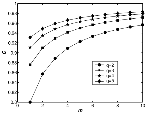
Figure 4: The dependence relation of $C$ on $q$ and $m$.

It can be easily proved that for arbitrary fixed $m$, $\overline{C}_{t}$ increases with $q$, and that for arbitrary fixed $q$, $\overline{C}_{t}$ increases with $m$. In the infinite network order limit ($N_{t}\rightarrow\infty$), Eq. (26) converges to a nonzero value $C$. When $q=2$, for $m=1$, 2, 3 and 4, $C$ equal to 0.8000, 0.8571 0.8889 and 0.9091, respectively. When $m=2$, for $q=2$, 3, 4 and 5, $C$ are 0.8571, 0.9100, 0.9348 and 0.9490, respectively. Therefore, the clustering coefficient of our networks is very high. Moreover, similarly to the degree exponent $\gamma$, clustering coefficient $C$ is determined by $q$ and $m$. Figure 4 shows the dependence of $C$ on $q$ and $m$.

Diameter. In what follows, the notations $\lceil x\rceil$ and $\lfloor x\rfloor$ express the integers obtained by rounding $x$ to the nearest integers towards infinity and minus infinity, respectively. Now we compute the diameter of $R(q,t)$, denoted $Diam(R(q,t))$ for $q\geq 3$ ($q=2$ is a particular case that is treated separately in the last subsection):

Step 0. The diameter is $1$.

Steps 1 to $\lceil\frac{q+1}{2}\rceil-1$. In this case, the diameter is 2, since any new node is by construction connected to a $q$-clique forming a $(q+1)$-clique, and since any $(q+1)$-clique during those steps contains at least $\lceil\frac{q+1}{2}\rceil$ ($q$ even) or $\lceil\frac{q+1}{2}\rceil$+1 ($q$ odd) nodes from the initial $(q+1)$-clique $R(q,0)$ obtained after step 0. Hence, any two newly added nodes $u$ and $v$ will be connected respectively to sets $S_{u}$ and $S_{v}$, with $S_{u}\subseteq V(R(q,0))$ and $S_{v}\subseteq V(R(q,0))$, where $V(R(q,0))$ is the node set of $R(q,0)$; however, since $|S_{u}|\geq\lceil\frac{q+1}{2}\rceil$ ($q$ even) and $|S_{v}|\geq\lceil\frac{q+1}{2}\rceil$+1 ($q$ odd), where $|S|$ denotes the number of elements in set $S$, we conclude that $S_{u}\cap S_{v}\neq{\O}$, and thus the diameter is 2.

Steps $\lceil\frac{q+1}{2}\rceil$ to $q$. In any of these steps, some newly added nodes might not share a neighbor in the original $(q+1)$-clique $R(q,0)$; however, any newly added node is connected to at least one node of the initial $(q+1)$-clique $R(q,0)$. Thus, the diameter is equal to 3.

Further steps. Similar to the case of $q=2$, we call “outer” nodes the nodes which are connected to a $q$-clique that did not exist at previous steps. Clearly, at each step, the diameter depends on the distances between outer nodes. Now, at any step $t\geq q+1$, an outer node cannot be connected with two or more nodes that were created during the same step $0<t^{\prime}\leq t-1$. Moreover, by construction no two nodes that were created during a given step are neighbors, thus they cannot be part of the same $q$-clique. Therefore, for any step $t\geq q+1$, some outer nodes are connected with nodes that appeared at pairwise different steps. Thus, if $v_{t}$ denotes an outer node that was created at step $t$, then $v_{t}$ is connected to nodes $v_{i}$s, $1\leq i\leq t-1$, where all the $i$s are pairwise distinct. We conclude that $v_{t}$ is necessarily connected to a node that was created at a step $t_{0}\leq t-q$. If we repeat this argument, then we obtain an upper bound on the distance from $v_{t}$ to the initial $(q+1)$-clique $R(q,0)$. Let $t=\alpha q+p$, where $1\leq p\leq q$. Then, we see that $v_{t}$ is at distance at most $\alpha+1$ from a node in $R(q,t)$. Hence any two nodes $v_{t}$ and $w_{t}$ in $R(q,0)$ lie at distance at most $2(\alpha+1)+1$ ; however, depending on $p$, this distance can be reduced by 1, since when $p\leq\lceil\frac{q+1}{2}\rceil-1$, we know that two nodes created at step $p$ share at least a neighbor in $R(q,0)$. Thus, when $1\leq p\leq\lceil\frac{q+1}{2}\rceil-1$, $Diam(R(q,t))\leq 2(\alpha+1)$, while when $\lceil\frac{q+1}{2}\rceil\leq p\leq q$, $Diam(R(q,t))\leq 2(\alpha+1)+1$. One can see that these bounds can be reached by pairs of outer nodes created at step $t$. More precisely, those two nodes $v_{t}$ and $w_{t}$ share the property that they are connected to $q$ nodes that appeared respectively at steps $t-1,t-2,\ldots t-q$.

Based on the above arguments, one can easily see that for $t>q$, the diameter increases by 2 every $q$ steps. More precisely, we have the following result, for any $q\geq 3$ and $t\geq 1$ (when $t=0$, the diameter is clearly equal to 1):

$$Diam(R(q,t))=2(\lfloor\frac{t-1}{q}\rfloor+1)+f(q,t),$$

where $f(q,t)=0$ if $t-\lfloor\frac{t-1}{q}\rfloor q\leq\lceil\frac{q+1}{2}\rceil-1$, and 1 otherwise. When $t$ gets large, $Diam(R(q,t))\sim\frac{2t}{q}$, while $N_{t}\sim(mq+1)^{t}$, thus the diameter grows logarithmically with the number of nodes.

It is easy to see that these cases of $q\geq 3$ have very similar topological properties to the case $q=2$. Additionally, for the cases of $q\geq 3$, the networks will again be disassortative with respect to degree because of the lack of links between nodes with the same degree; the second moment of degree distribution $\langle k^{2}\rangle$ will also diverge, which is due to the fat tail of the degree distribution.

4 Conclusion and discussion

To sum up, we have proposed and investigated a deterministic network model, which is constructed in a recursive fashion. Our model is actually a tunable generalization of the growing deterministic scale-free networks introduced in Ref. [10]. Aside from their deterministic structures, the statistical properties of the resulting networks are equivalent with the random models that are commonly used to generate scale-free networks [4, 5, 6, 7]. We have obtained the exact results for degree distribution and clustering coefficient, as well as the diameter, which agree well with large amount of real observations [4, 5, 6, 7]. The degree exponent can be adjusted, the clustering coefficient is very large, and the diameter is small. Therefore, out model may perform well in mimicking a variety of scale-free networks in real-life world. Moreover, our networks consist of cliques, which has been observed in variety of the real-world networks, such as movie actor collaboration networks, scientific collaboration networks and networks of company directors [4, 5, 6, 7].

Acknowledgment

This research was supported in part by the National Natural Science Foundation of China (NNSFC) under Grant Nos. 60373019, 60573183, and 90612007. Lili Rong gratefully acknowledges partial support from NNSFC under Grant Nos. 70431001 and 70571011. The authors thank the anonymous referees for their valuable comments and suggestions.

References

- [1] D. J. Watts and H. Strogatz, Nature (London) 393, 440 (1998).
- [2] A.-L. Barabási and R. Albert, Science 286, 509 (1999).
- [3] S. H. Strogatz, Nature 410, 268 (2001).
- [4] R. Albert and A.-L. Barabási, Rev. Mod. Phys. 74, 47 (2002).
- [5] S. N. Dorogvtsev and J.F.F. Mendes, Adv. Phys. 51, 1079 (2002).
- [6] M. E. J. Newman, SIAM Review 45, 167 (2003).
- [7] S Boccaletti, V Latora, Y Moreno, M. Chavezf, and D.-U. Hwanga, Physics Report 424, 175 (2006).
- [8] A.-L. Barabási, E. Ravasz, and T. Vicsek, Physica A 299, 559 (2001).
- [9] K. Iguchi and H. Yamada, Phys. Rev. E 71, 036144 (2005).
- [10] S. N. Dorogovtsev, A. V. Goltsev, and J. F. F. Mendes, Phys. Rev. E 65, 066122 (2002).
- [11] F. Comellas, G. Fertin and A. Raspaud, Phys. Rev. E 69, 037104 (2004).
- [12] S. Jung, S. Kim, and B. Kahng, Phys. Rev. E 65, 056101 (2002).
- [13] E. Ravasz, A.L. Somera, D.A. Mongru, Z.N. Oltvai, and A.-L. Barabási, Science 297, 1551 (2002).
- [14] E. Ravasz and A.-L. Barabási, Phys. Rev. E 67, 026112 (2003).
- [15] J. D. Noh, Phys. Rev. E 67, 045103 (2003).
- [16] J. C. Nacher, N. Ueda, M. Kanehisa and T. Akutsu, Phys. Rev. E 71, 036132 (2005).
- [17] J. S. Andrade Jr., H. J. Herrmann, R. F. S. Andrade and L. R. da Silva, Phys. Rev. Lett. 94, 018702 (2005).
- [18] J. P. K. Doye and C. P. Massen, Phys. Rev. E 71, 016128 (2005).
- [19] H. Rozenfeld, J. Kirk, E. Bollt and D. ben-Avraham, J. Phys. A 38, 4589 (2005).
- [20] E. Bollt, D. ben-Avraham, New Journal of Physics 7, 26 (2005).
- [21] M. Hinczewski and A. N. Berker, Phys. Rev. E 73, 066126 (2006).
- [22] Z. Z. Zhang, F. Comellas, G. Fertin and L. L. Rong, J. Phys. A 39, 1811 (2006).
- [23] Z. Z. Zhang, L. L. Rong, and Shuigeng Zhou, Phys. Rev. E, 74, 046105 (2006).
- [24] F. Comellas, J. Ozón, and J. G. Peters, Inf. Process. Lett., 76, 83 (2000)
- [25] F. Comellas and M. Sampels, Physica A 309, 231 (2002).
- [26] Z. Z. Zhang, L. L. Rong and C. H. Guo, Physica A 363, 567 (2006).
- [27] Z. Z. Zhang, L. L. Rong and F. Comellas, J. Phys. A 39, 3253 (2006).
- [28] T. Zhou, B. H. Wang, P. M. Hui and K. P. Chan, Physica A 367, 613 (2006).
- [29] G. Corso, Phys. Rev. E 69, 036106 (2004).
- [30] J. D. Achter, Phys. Rev. E 70, 058103 (2004).
- [31] A. K. Chandra, S Dasgupta, Physica A, Physica A 357, 436 (2005).
- [32] T. Zhou, G. Yan, and B. H. Wang, Phys. Rev. E 71, 046141 (2005).
- [33] Z. Z. Zhang, L. L. Rong and F. Comellas, Physica A 364, 610 (2006).
- [34] R. F. S. Andrade and H. J. Herrmann, Phys. Rev. E 71, 056131 (2005).
- [35] P. G. Lind, J.A.C. Gallas, and H.J. Herrmann, Phys. Rev. E 70, 056207 (2004).
- [36] R.F.S. Andrade, J.G.V. Miranda, Physica A 356, 1 (2005).
- [37] R. B. Griffiths and M. Kaufman, Phys. Rev. B 26, 5022 (1982).
- [38] R. Pastor-Satorras and A. Vespignani, Phys. Rev. Lett. 86, 3200 (2001).
- [39] R. Pastor-Satorras and A. Vespignani, Phys. Rev. E 63, 066117 (2001).
- [40] R. Albert, H. Jeong, and A.-L. Barabási, Nature (London) 406, 378 (2000).
- [41] R. Cohen, K. Erez, D. ben Avraham, and S. Havlin, Phys. Rev. Lett. 86, 3682 (2001).
- [42] S. Maslov and K. Sneppen, Science 296, 910 (2002).
- [43] R. Pastor-Satorras, A. Vázquez and A. Vespignani, Phys. Rev. Lett. 87, 258701 (2001).
- [44] A. Vázquez, R. Pastor-Satorras and A. Vespignani, Phys. Rev. E 65, 066130 (2002).
- [45] M. E. J. Newman, Phys. Rev. Lett. 89, 208701 (2002).
- [46] M. E. J. Newman, Phys. Rev. E 67, 026126 (2003).