Deterministic scale-free networks created in a recursive manner

Abstract

In a recursive way and by including a parameter, we introduce a family of deterministic scale-free networks. The resulting networks exhibit small-world effects. We calculate the exact results for the degree exponent, the clustering coefficient and the diameter. The major points of our results indicate: the degree exponent can be adjusted; the clustering coefficient of each individual vertex is inversely proportional to its degree and the average clustering coefficient of all vertices approaches to a nonzero value in the infinite network order; and the diameter grows logarithmically with the number of network vertices.

I Introduction

Since the two seminal papers by Watts and Strogatz on small-world networks WaSt98 and Barabási and Albert on scale-free networks BaAl99 , we have witnessed a considerable efforts devoted to characterization and understanding of complex networks, which describe many systems in nature and society. In the past few years, there has been a substantial amount of interest in network structure and function from a wide circle of researchers St01 ; AlBa02 ; DoMe02 ; Ne03 ; SaVe04 . One particular question that has attracted an exceptional amount of attention concerns the structure of networks that are evolving over time. A number of network models have been proposed, which convincingly reproduce some or all features of real-life systems St01 ; AlBa02 ; DoMe02 ; Ne03 ; SaVe04 .

Most of the precious models are stochastic St01 ; AlBa02 ; DoMe02 ; Ne03 ; SaVe04 . However, because of their advantages, deterministic networks have also received much attention BaRaVi01 ; IgYa05 ; DoGoMe02 ; JuKiKa02 ; CoFeRa04 ; RaSoMoOlBa02 ; RaBa03 ; No03 ; NaUeKaAk05 ; AnHeAnSi05 ; DoMa05 ; ZhCoFeRo05 ; CoOzPe00 ; CoSa02 ; ZhRoGo05 ; ZhWaHuCh04 . First, the method of generating deterministic networks makes it easier to gain a visual understanding of how networks are shaped, and how do different vertices relate to each other; moreover, deterministic networks allow to compute analytically their properties: degree distribution, clustering coefficient, average path length, diameter, betweenness, modularity and adjacency matrix whose eigenvalue spectrum characterizes the topology BaRaVi01 ; IgYa05 ; DoGoMe02 ; JuKiKa02 ; CoFeRa04 ; RaSoMoOlBa02 ; RaBa03 ; No03 ; NaUeKaAk05 ; AnHeAnSi05 ; DoMa05 ; ZhCoFeRo05 ; CoOzPe00 ; CoSa02 ; ZhRoGo05 ; ZhWaHuCh04 .

The first model for deterministic scare-free networks was proposed by Barabási et al. in Ref. BaRaVi01 and was intensively studied in Ref. IgYa05 . Another elegant model, called pseudofractal scale-free web (PSW) DoGoMe02 , was introduced by Dorogovtsev and Mendes, and was extended by Comellas et al. in Ref. CoFeRa04 . Based on a similar idea of PSW, Jung et al. presented a class of recursive trees JuKiKa02 . Additionally, in order to discuss modularity, Ravasz et al. proposed a hierarchical network model RaSoMoOlBa02 ; RaBa03 , the exact scaling properties and extensive study of which were reported in Refs. No03 and NaUeKaAk05 , respectively. Recently, In relation to the problem of Apollonian space-filing packing, Andrade et al. introduced Apollonian networks AnHeAnSi05 which were also proposed by Doye and Massen in Ref. DoMa05 and have been intensively investigated ZhCoFeRo05 ; ZhYaWa05 ; ZhRoCo05 ; ZhCo05 . Except for above models, deterministic networks can be created by various techniques: modification of some regular graphs CoOzPe00 , addition and product of graphs CoSa02 , edge iterations ZhRoGo05 and other mathematical methods as in Ref. ZhWaHuCh04 .

As mentioned by Barabási et al., it would be of major theoretical interest to construct deterministic models that lead to scale-free networks BaRaVi01 . In this paper, we do an extensive study on pseudofractal scale-free web DoGoMe02 and the recursive graphs (RG) CoFeRa04 . In a simple recursive way we propose a general model for PSW and RG by including a parameter, with PSW and RG as particular cases of the present model. The deterministic construction of our model enables one to obtain the analytic solutions for some main structure properties: degree distribution, clustering coefficient and diameter. By adjusting the parameter, we can obtain a variety of scale-free networks.

II The network construction

Before introducing our networks we give the following definitions on a graph. The term size refers to the number of edges in a graph. The number of vertices in a graph is called its order. When two vertices of a graph are connected by an edge, these vertices are said to be adjacent, and the edge is said to join them. A complete graph is a graph in which all vertices are adjacent to one another. Thus, in a complete graph, every possible edge is present. The complete graph with $q$ vertices is denoted as $K_{q}$ (also referred in the literature as $q$-clique; see We01 ). Two graphs are isomorphic when the vertices of one can be relabeled to match the vertices of the other in a way that preserves adjacency. So all $q$-cliques are isomorphic to one another.

The network is constructed in a recursive way. We denote the network after $t$ steps by $R(q,t)$, $q\geq 2,t\geq 0$ (see Fig. 1). Then the network at step $t$ is constructed as follows: For $t=0$, $R(q,0)$ is a complete graph $K_{q+1}$ (or $(q+1)$-clique) consist of $q+1$ $q$-cliques), and $R(q,0)$ has $q+1$ vertices and $q(q+1)/2$ edges. For $t\geq 1$, $R(q,t)$ is obtained from $R(q,t-1)$ by adding $m$ new vertices for each of its existing subgraphs isomorphic to a $q$-clique, and each new vertex is connected to all the vertices of this subgraph. In the special case $m=1$, it is reduced to the network described in Ref. CoFeRa04 which is a generalization of pseudofractal scale-free web DoGoMe02 .

Figure 1: Scheme of the growth of the deterministic network for the case of $q=2$ and $m=2$. Only the first three steps are shown.

Let $n_{v}(t)$ and $n_{e}(t)$ be the number of vertices and edges created at step $t$, respectively. Denote $K_{q,t}$ as the total number of $q$-cliques in the whole network at step $t$. Note that the addition of each new vertex leads to $q$ new $q$-cliques and $q$ new edges. By construction, we have $n_{e}(t)=qn_{v}(t)$, $n_{v}(t)=mK_{q,t-1}$ and $K_{q,t}=K_{q,t-1}+qn_{v}(t)$. Thus one can easily obtain $K_{q,t}=(mq+1)K_{q,t-1}=(q+1)(mq+1)^{t}$ ($t\geq 0$), $n_{v}(t)=m(q+1)(mq+1)^{t-1}$ ($t>0$) and $n_{e}(t)=mq(q+1)(mq+1)^{t-1}$ ($t>0$). So the number of network vertices increases exponentially with time. From above results, we can easily compute the size and order of the networks. The total number of vertices $N_{t}$ and edges $|E|_{t}$ present at step $t$ is

$$N_{t}=\sum_{t_{i}=0}^{t}n_{v}(t_{i})=\frac{(q+1)[(mq+1)^{t}+q-1]}{q}$$ (1)

and

$$|E|_{t}=\sum_{t_{i}=0}^{t}n_{e}(t_{i})=(q+1)(mq+1)^{t}+\frac{(q+1)(q-2)}{2},$$ (2)

respectively. So for large $t$, The average degree $\overline{k}_{t}=\frac{2|E|_{t}}{N_{t}}$ is approximately $2q$.

III Characteristics of the networks

III.1 Degree distribution

When a new vertex $i$ is added to the graph at step $t_{i}$, it has degree $q$ and forms $q$ new $q$-cliques. Let $n_{q}(i,t)$ be the total number of $q$-cliques at step $t$ that will created new vertices connected to the vertex $i$ at step $t+1$. So at step $t_{i}$, $n_{q}(i,t_{i})=q$. By construction, we can see that in the subsequent steps each new neighbor of $i$ generated $q-1$ new $q$-cliques with $i$ as one vertex of them. Let $k_{i}(t)$ be the degree of $i$ at step $t$. It is not difficult to find following relations for $t>t_{i}+1$:

$$\Delta k_{i}(t)=k_{i}(t)-k_{i}(t-1)=mn_{q}(i,t-1)$$ (3)

and

$$n_{q}(i,t)=n_{q}(i,t-1)+(q-1)\Delta k_{i}(t).$$ (4)

From the above two equations, we can derive $n_{q}(i,t_{i})=[m(q-1)+1]n_{q}(i,t_{i}-1)$. Considering $n_{q}(i,t_{i})=q$, we obtain $n_{q}(i,t)=q[m(q-1)+1]^{t-t_{i}}$ and $\Delta k_{i}(t)=mq[m(q-1)+1]^{t-t_{i}-1}$. Then the degree $k_{i}(t)$ of vertex $i$ at time $t$ is

$$k_{i}(t) = k_{i}(t_{i})+\sum_{t_{h}=t_{i}+1}^{t}{\Delta k_{i}(t_{h})}$$ (5)

$$= \frac{q[m(q-1)+1]^{t-t_{i}}+q^{2}-2q}{q-1}.$$

Since the degree of each vertex has been obtained explicitly as in Eq. (5), we can get the degree distribution via its cumulative distribution, i.e. $P_{cum}(k)\equiv\sum_{k^{\prime}\geq k}N(k^{\prime},t)/N_{t}\sim k^{1-\gamma}$, where $N(k^{\prime},t)$ denotes the number of vertices with degree $k^{\prime}$. The analytic computation details are given as follows. For a degree $k$

$$k=\frac{q[m(q-1)+1]^{t-j}+q^{2}-2q}{q-1},$$ (6)

there are $n_{v}(j)=m(q+1)(qm+1)^{t-1}$ vertices with this exact degree, all of which were born at step $j$. All vertices with birth time at $j$ or earlier have this and a higher degree. So we have

$$\sum_{k^{\prime}\geq k}N(k^{\prime},t)=\sum_{s=0}^{j}n_{v}(s)=\frac{(q+1)[(mq+1)^{j}+q-1]}{q}.\\$$

As the total number of vertices at step $t$ is given in Eq. (1) we have

$$\left[\frac{q[m(q-1)+1]^{t-j}+q^{2}-2q}{q-1}\right]^{1-\gamma}\\ =\frac{\frac{(q+1)[(mq+1)^{j}+q-1]}{q}}{\frac{(q+1)[(mq+1)^{t}+q-1]}{q}}.\\$$

Therefore, for large $t$ we obtain

$$\left[[m(q-1)+1]^{t-j}\right]^{1-\gamma}=(mq+1)^{j-t}$$ (7)

and

$$\gamma\approx 1+\frac{\ln(mq+1)}{\ln[m(q-1)+1]}.$$ (8)

For the particular case of $m=1$, Eq. (8) recovers the results previously obtained in Ref. CoFeRa04 .

III.2 Clustering coefficient

The clustering coefficient WaSt98 $C_{i}$ of vertex $i$ is defined as the ratio between the number of edges $e_{i}$ that actually exist among the $k_{i}$ neighbors of vertex $i$ and its maximum possible value, $k_{i}(k_{i}-1)/2$, i.e., $C_{i}=2e_{i}/k_{i}(k_{i}-1)$. The clustering coefficient of the whole network is the average of $C_{i}^{\prime}s$ over all vertices in the graph.

For our networks, the analytical expressions for clustering coefficient $C(k)$ of the individual vertex with degree $k$ can be derived exactly. When a vertex is created it is connected to all the vertices of a $q$-clique whose vertices are completely interconnected. Its degree and clustering coefficient are $q$ and 1, respectively. In the following steps, if its degree increases one by a newly created vertex connecting to it, then there must be $q-1$ existing neighbors of it attaching to the new vertex at the same time. Thus for a vertex of degree $k$, we have

$$C(k)={{{q(q-1)\over 2}+(q-1)(k-q)}\over{k(k-1)\over 2}}=\frac{2(q-1)(k-\frac{q}{2})}{k(k-1)},$$ (9)

which depends on degree $k$ and $q$. For $k\gg q$, the $C(k)$ is inversely proportional to degree. The scaling $C(k)\sim k^{-1}$ has been found for some network models DoGoMe02 ; CoFeRa04 ; RaBa03 ; No03 ; AnHeAnSi05 ; DoMa05 ; ZhCoFeRo05 ; ZhYaWa05 ; ZhRoCo05 , and has also observed in several real-life networks RaBa03 .

Using Eq. (9), we can obtain the clustering $\overline{C}_{t}$ of the networks at step $t$:

$$\overline{C}_{t}=\frac{1}{N_{t}}\sum_{r=0}^{t}\frac{2(q-1)(D_{r}-\frac{q}{2})n_{v}(r)}{D_{r}(D_{r}-1)},$$ (10)

where the sum is the total of clustering coefficient for all vertices and $D_{r}=\frac{q[m(q-1)+1]^{t-r}+q^{2}-2q}{q-1}$ shown by Eq. (5) is the degree of the vertices created at step $r$.

It can be easily proved that for arbitrary fixed $m$, $\overline{C}_{t}$ increases with $q$, and that for arbitrary fixed $q$, $\overline{C}_{t}$ increases with $m$. In the infinite network order limit ($N_{t}\rightarrow\infty$), Eq. (10) converges to a nonzero value $C$. When $q=2$, for $m=1$, 2, 3 and 4, $C$ equal to 0.8000, 0.8571 0.8889 and 0.9091, respectively. When $m=2$, for $q=2$, 3, 4 and 5, $C$ are 0.8571, 0.9100, 0.9348 and 0.9490, respectively. Therefore, the clustering coefficient of our networks is very high. Moreover, similarly to the degree exponent $\gamma$, clustering coefficient $C$ is determined by $q$ and $m$. Fig. 2 shows the dependence of $C$ on $q$ and $m$.

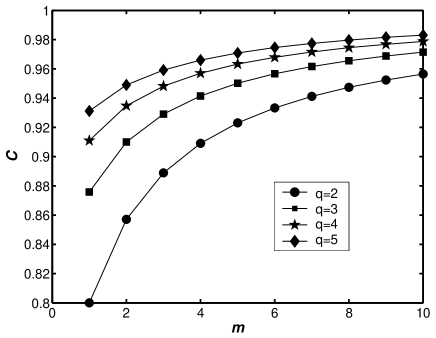
Figure 2: The dependence relation of $C$ on $q$ and $m$.

III.3 Diameter

The diameter of a network characterizes the maximum communication delay in the network and is defined as the maximum of shortest path between all pairs of vertices. In what follows, the notations $\lceil x\rceil$ and $\lfloor x\rfloor$ express the integers obtained by rounding $x$ to the nearest integers towards infinity and minus infinity, respectively. Now we compute the diameter of $R(q,t)$, denoted $Diam(R(q,t))$ for $q\geq 3$ ($q=2$ is a particular case that is treated separately):

Step 0. The diameter is $1$.

Steps 1 to $\lceil\frac{q+1}{2}\rceil-1$. In this case, the diameter is 2, since any new vertex is by construction connected to a $q$-clique forming a $(q+1)$-clique, and since any $(q+1)$-clique during those steps contains at least $\lceil\frac{q+1}{2}\rceil$ ($q$ even) or $\lceil\frac{q+1}{2}\rceil$+1 ($q$ odd) vertices from the initial $(q+1)$-clique $R(q,0)$ obtained after step 0. Hence, any two newly added vertices $u$ and $v$ will be connected respectively to sets $S_{u}$ and $S_{v}$, with $S_{u}\subseteq V(R(q,0))$ and $S_{v}\subseteq V(R(q,0))$, where $V(R(q,0))$ is the vertex set of $R(q,0)$; however, since $|S_{u}|\geq\lceil\frac{q+1}{2}\rceil$ ($q$ even) and $|S_{v}|\geq\lceil\frac{q+1}{2}\rceil$+1 ($q$ odd), where $|S|$ denotes the number of elements in set $S$, we conclude that $S_{u}\cap S_{v}\neq{\O}$, and thus the diameter is 2.

Steps $\lceil\frac{q+1}{2}\rceil$ to $q$. In any of those steps, some newly added vertices might not share a neighbor in the original $(q+1)$-clique $R(q,0)$; however, any newly added vertex is connected to at least one vertex of the initial $(q+1)$-clique $R(q,0)$. Thus, the diameter is equal to 3.

Further steps. In order to simplify the analysis, we first note that it is unnecessary to look at all the vertices in the graph in order to find the diameter. In other words, some vertices added at a given step can be ignored, because they do not increase the diameter from the previous step. These vertices are those that connect to vertices that already formed a $(q+1)$-clique in one or several of the previous steps: indeed, for these vertices we know that a similar construction has been done in previous steps, so we can ignore them for the computation of the diameter. Let us call “outer” vertices the vertices which are connected to a $q$-clique that did not exist previously. Clearly, at each step, the diameter depends on the distances between outer vertices.

Now, at any step $t\geq q+1$, we note that an outer vertex cannot be connected with two or more vertices that were created during the same step $0<t^{\prime}\leq t-1$. Moreover, by construction no two vertices that were created during a given step are neighbors, thus they cannot be part of the same $q$-clique. Therefore, for any step $t\geq q+1$, some outer vertices are connected with vertices that appeared at pairwise different steps. Thus, if $v_{t}$ denotes an outer vertex that was created at step $t$, then $v_{t}$ is connected to vertices $v_{i}$s, $1\leq i\leq t-1$, where all the $i$s are pairwise distinct. We conclude that $v_{t}$ is necessarily connected to a vertex that was created at a step $t_{0}\leq t-q$. If we repeat this argument, then we obtain an upper bound on the distance from $v_{t}$ to the initial $(q+1)$-clique $R(q,0)$. Let $t=\alpha q+p$, where $1\leq p\leq q$. Then, we see that $v_{t}$ is at distance at most $\alpha+1$ from a vertex in $R(q,t)$. Hence any two vertices $v_{t}$ and $w_{t}$ in $R(q,0)$ lie at distance at most $2(\alpha+1)+1$ ; however, depending on $p$, this distance can be reduced by 1, since when $p\leq\lceil\frac{q+1}{2}\rceil-1$, we know that two vertices created at step $p$ share at least a neighbor in $R(q,0)$. Thus, when $1\leq p\leq\lceil\frac{q+1}{2}\rceil-1$, $Diam(R(q,t))\leq 2(\alpha+1)$, while when $\lceil\frac{q+1}{2}\rceil\leq p\leq q$, $Diam(R(q,t))\leq 2(\alpha+1)+1$. One can see that these bounds can be reached by pairs of outer vertices created at step $t$. More precisely, those two vertices $v_{t}$ and $w_{t}$ share the property that they are connected to $q$ vertices that appeared respectively at steps $t-1,t-2,\ldots t-q$.

Based on the above arguments, one can easily see that for $t>q$, the diameter increases by 2 every $q$ steps. More precisely, we have the following result, for any $q\geq 3$ and $t\geq 1$ (when $t=0$, the diameter is clearly equal to 1):

$$Diam(K(q,t))=2(\lfloor\frac{t-1}{q}\rfloor+1)+f(q,t),$$

where $f(q,t)=0$ if $t-\lfloor\frac{t-1}{q}\rfloor q\leq\lceil\frac{q+1}{2}\rceil-1$, and 1 otherwise. When $t$ gets large, $Diam(R(q,t))\sim\frac{2t}{q}$, while $N_{t}\sim(mq+1)^{t}$, thus the diameter grows logarithmically with the number of vertices.

For $q=2$, the argument is similar: when $t=0$ (resp. $t=1$), the diameter is equal to 1 (resp. 2). Now consider two outer vertices created at step $t\geq 2$, say $v_{t}$ and $w_{t}$. Then $v_{t}$ is connected to two vertices, and one of them must have been created before or during step $t-2$. We repeat this argument, and we end up with 2 cases: (1) $t=2m$ is even. Then, if we make $m$ “jumps”, from $v_{t}$ we arrive in $R(2,0)$, in which we can reach any $w_{t}$ by using an edge of $R(2,0)$ and making $m$ jumps to $w_{t}$ in a similar way. Thus $Diam(R(2,2m))\leq 2m+1$. (2) $t=2m+1$ is odd. In this case we can stop after $m$ jumps at $R(2,1)$, for which we now that the diameter is 2, and make $m$ jumps in a similar way to reach $w_{t}$. Thus $Diam(R(2,2m+1))\leq 2m+2$. As previously, it easily seen that the bound can be reached for some pairs of vertices.

Hence, formally, $Diam(R(2,t))=t+1$ for any $t\geq 0$. In this particular case, the network order $N_{t}\sim(2m+1)^{t}$, thus $Diam(R(2,t))$ also increases logarithmically with network order.

IV Conclusion and discussion

In summary, we have proposed and studied a network model constructed in a recursive fashion. At each time step, each already existing $q$-clique generates $m$ new vertices. The process results in a serial of networks with two published papers  DoGoMe02 ; CoFeRa04 as special cases of them. We have obtained the analytical results for degree exponent, clustering coefficient and diameter. The degree exponent and the clustering coefficient may be adjusted to various values by tuning the parameter $m$. Therefore, they may perform well in mimicking a variety of scale-free networks in real world. Moreover, in a similar way, one can easily consider other variations, for example, at each step not all cliques of a network but only some of them generate vertices, which also allow a rich structure and flexibility in the control of degree exponent, clustering coefficient and other properties. Details of the analytical solution for these variants will be addressed elsewhere.

This research was supported by the National Natural Science Foundation of China under Grant No. 70431001.

References

- (1) D. J. Watts and H. Strogatz, Nature (London) 393, 440 (1998).
- (2) A.-L. Barabási and R. Albert, Science 286, 509 (1999).
- (3) S. H. Strogatz, Nature 410, 268 (2001).
- (4) R. Albert and A.-L. Barabási, Rev. Mod. Phys. 74, 47 (2002).
- (5) S. N. Dorogvtsev and J.F.F. Mendes, Adv. Phys. 51, 1079 (2002).
- (6) M. E. J. Newman, SIAM Review 45, 167 (2003).
- (7) R. Pastor-Satorras and A. Vespignani, Evolution and Structure of the Internet: A Statistical Physics Approach (Cambridge University Press, Cambridge, England, 2004).
- (8) A.-L. Barabási, E. Ravasz, and T. Vicsek, Physica A 299, 559 (2001).
- (9) K. Iguchi and H. Yamada, Phys. Rev. E 71, 036144 (2005).
- (10) S. N. Dorogovtsev, A. V. Goltsev, and J. F. F. Mendes, Phys. Rev. E 65, 066122 (2002).
- (11) F. Comellas, G. Fertin and A. Raspaud, Phys. Rev. E 69, 037104 (2004).
- (12) S. Jung, S. Kim, and B. Kahng, Phys. Rev. E 65, 056101 (2002).
- (13) E. Ravasz, A.L. Somera, D.A. Mongru, Z.N. Oltvai, and A.-L. Barabási, Science 297, 1551 (2002).
- (14) E. Ravasz and A.-L. Barabási, Phys. Rev. E 67, 026112 (2003).
- (15) J. D. Noh, Phys. Rev. E 67, 045103 (2003).
- (16) J. C. Nacher, N. Ueda, M. Kanehisa and T. Akutsu, Phys. Rev. E 71, 036132 (2005).
- (17) J. S. Andrade Jr., H. J. Herrmann, R. F. S. Andrade and L. R. da Silva, Phys. Rev. Lett. 94, 018702 (2005).
- (18) J. P. K. Doye and C. P. Massen. Phys. Rev. E 71, 016128 (2005).
- (19) Z. Z. Zhang, F. Comellas, G. Fertin and L. L. Rong, e-print cond-mat/0503316.
- (20) T. Zhou, G. Yan, and B. H. Wang, Phys. Rev. E 71, 046141 (2005).
- (21) Z. Z. Zhang, L. L. Rong and F. Comellas, e-print cond-mat/0502591.
- (22) Z. Z. Zhang and L. L. Rong, e-print cond-mat/0511609.
- (23) F. Comellas, J. Ozón, and J. G. Peters, Inf. Process. Lett., 76, 83 (2000)
- (24) F. Comellas and M. Sampels, Physica A 309, 231 (2002).
- (25) Z. Z. Zhang, L. L. Rong and C. H. Guo, e-print cond-mat/0502335.
- (26) T. Zhou, B. H. Wang, P. M. Hui and K. P. Chan, e-print cond-mat/0405258.
- (27) D.B. West, Introduction to Graph Theory (Prentice-Hall, Upper Saddle River, NJ, 2001).