Orbital magnetization in crystalline solids:
Multi-band insulators, Chern insulators, and metals

Abstract

We derive a multi-band formulation of the orbital magnetization in a normal periodic insulator (i.e., one in which the Chern invariant, or in 2d the Chern number, vanishes). Following the approach used recently to develop the single-band formalism [T. Thonhauser, D. Ceresoli, D. Vanderbilt, and R. Resta, Phys. Rev. Lett. 95, 137205 (2005)], we work in the Wannier representation and find that the magnetization is comprised of two contributions, an obvious one associated with the internal circulation of bulk-like Wannier functions in the interior and an unexpected one arising from net currents carried by Wannier functions near the surface. Unlike the single-band case, where each of these contributions is separately gauge-invariant, in the multi-band formulation only the sum of both terms is gauge-invariant. Our final expression for the orbital magnetization can be rewritten as a bulk property in terms of Bloch functions, making it simple to implement in modern code packages. The reciprocal-space expression is evaluated for 2d model systems and the results are verified by comparing to the magnetization computed for finite samples cut from the bulk. Finally, while our formal proof is limited to normal insulators, we also present a heuristic extension to Chern insulators (having nonzero Chern invariant) and to metals. The validity of this extension is again tested by comparing to the magnetization of finite samples cut from the bulk for 2d model systems. We find excellent agreement, thus providing strong empirical evidence in favor of the validity of the heuristic formula.

I Introduction

During the last decade, charge and spin transport phenomena in magnetic materials and nanostructures have attracted much interest due to their important role for spintronic devices.fabian04 An adequate description of magnetism in these materials, however, should not only include the spin contribution, but also should account for effects originating in the orbital magnetization. In light of this, it is surprising that the theory of orbital magnetization has long remained underdeveloped. Earlier attempts to develop such a theory used linear-response methods, which allow calculations of magnetization changes,linear ; Sebastiani01 ; Mauri ; Sebastiani02 but not of the magnetization itself.

Just recently, a new approach using Wannier functions (WFs) has been proposed,ChemPhysChem ; Thonhauser05 which nicely parallels the analogous case of the electric polarization. The primary difficulty in both cases is that the position operator ${\bf r}$ is not well-defined in the Bloch representation. Since WFs are exponentially localized in an insulator, this difficulty disappears if the problem is reformulated in the Wannier representation. For the polarization, this approach lead to the development of the modern theory of polarization in the early 1990s.KSV ; rap-a12 Similarly, in the case of the orbital magnetization, where the circulation operator ${{\bf r}}\times{{\bf v}}$ is ill-defined in the Bloch representation, the Wannier representation was used to derive a theory for the orbital magnetization of periodic insulators.Thonhauser05

While the formalism developed in Ref. Thonhauser05, lays a firm foundation for the orbital magnetization, its application is limited to certain systems, such as single-band models and insulators. In this paper we expand the applicability to a much wider class of systems by developing a corresponding multi-band formalism, essential for most “real” materials. This extension is nontrivial and the corresponding proof of gauge invariance is much more complex than for the single-band case. We proceed in two steps. First, we carry out a derivation for the case of an insulator with zero Chern invariant. Second, we give heuristic arguments for an extension of our formalism to metals and Chern insulators, i.e. systems with a non-zero Chern invariant, arriving at a formula identical to that proposed by Xiao, Shi and NiuXiao05 on the basis of semiclassical arguments. Chern insulators have been introduced into the theoretical literature by means of model Hamiltonians in 2d which break time-reversal (TR) symmetry without breaking translational symmetry, Haldane88 i.e., maintaining a vanishing macroscopic magnetic field. Despite the absence of a macroscopic field, Chern insulators share several properties with quantum-Hall systems, most notably the quantization of the transverse conductivity in 2d.Haldane88 To the best of our knowledge, there is no known experimental realization of a Chern insulator (in zero field) in either 2d or 3d, and the search for such a system remains a fascinating challenge.

Our extensions to metals and Chern insulators are heuristic and not based on an analytical proof. The fact that our final formula is identical to the one derived from the semiclassical wavepacket treatmentXiao05 is reassuring, but neither of these approaches can yet be said to constitute a “derivation” of the formula in the fully quantum context. Nevertheless, we provide strong numerical evidence of their validity, thus posing a theoretical challenge: how to provide an analytic proof of the heuristic formula, beyond the range of the semiclassical approximation, for both the metallic and Chern-insulating cases.

Before proceeding, we emphasize that the present work only addresses the question of how to compute the orbital magnetization for a given independent-particle Hamiltonian. Many interesting questions remain concerning which flavor of density-functional theory (DFT) or which exchange-correlation (XC) functional might give the most accurate orbital magnetization. While exact Kohn-Sham (KS) density (or spin-density) functional theory is guaranteed to yield the correct charge (or spin) density,DFT there is no reason to expect it to yield the correct orbital currents. The orbital magnetization, being defined in terms of surface currents, is not guaranteed to be correct either. A prescription that seems more suited to the present situation is that of Vignale and Rasolt,Vignale88 in which the spin-labeled density and current $\{n_{\sigma}({\bf r}),\;{\bf j}_{\sigma}({\bf r})\}$ are connected to corresponding scalar and vector potentials $\{V_{\sigma}({\bf r}),\;{\bf A}_{\sigma}({\bf r})\}$. However, it is an open question whether an approximate Vignale-Rasolt XC functional exists that can give improved values of magnetization in practice. While time-dependent density functional theory (TDDFT) is more developed,TDDFT this theory only establishes a connection between $n({\bf r},t)$ and $V({\bf r},t)$, and a knowledge of $n({\bf r},t)$ is only sufficient to determine the longitudinal part of ${\bf j}({\bf r},t)$, not the transverse part upon which the orbital magnetization depends. An alternative approach worthy of exploration is time-dependent current-density functional theory (TD-CDFT),TD-CDFT in which $\{n({\bf r},t),\;{\bf j}({\bf r},t)\}$ is connected to $\{V({\bf r},t),\;{\bf A}({\bf r},t)\}$. However, the present problem is essentially a static problem, and it is therefore unclear whether TD-CDFT would provide any practical advantage over the Vignale-Rasolt theory. Finally, it is worth remembering that even in standard DFT, the mapping from interacting density to non-interacting potential is sometimes pathological (e.g., a KS metal can represent an interacting insulator). In the present work, we bypass all these interesting issues, and only consider how to compute the magnetization for a given Kohn-Sham Hamiltonian arising from some unspecified version of DFT in the context of broken TR symmetry.

We have organized this paper as follows. In Sec. II we derive the multi-band theory of orbital magnetization in crystalline solids. After some definitions and generalities, we start by considering the orbital magnetization of a finite sample. The resulting expression is then transformed to reciprocal space and its gauge invariance is demonstrated. We then give a heuristic extension of our formalism to metals and Chern insulators. In Sec. III, numerical results for the orbital magnetization are presented for several different systems. We conclude in Sec. IV. Some details concerning the finite-difference evaluation of the magnetization and certain properties of the nonAbelian Berry curvature are deferred to two appendices.

II Theory

II.1 Generalities

Our basic starting point is a single-particle KS Hamiltonian DFT having the translational symmetry of the crystal, but having no TR symmetry: as said above, translational symmetry of the Hamiltonian implies vanishing of the macroscopic magnetic field. There may, however, be a microscopic magnetic field ${\bf B}$ that averages to zero over the unit cell, and we assume that a particular magnetic gauge has been chosen once and for all to represent this magnetic field. Wavevector ${\bf k}$ is a good quantum number under these conditions. This could be realized, for example, in systems in which the TR breaking comes about through the spontaneous development of ferromagnetic order or via spin-orbit coupling to a background of ordered local moments.Haldane88 ; Ohgushi00 ; Jungwirth02 ; Murakami03 ; Yao04 Notice that we carefully avoid referring to an externally applied field; such concept is legitimate only for a finite sample, free-standing in vacuo. Indeed, for a finite sample, the relationship between the externally applied field and the “internal” (or screened) one depends on the sample shape. For an extended sample in the thermodynamic limit, the only legitimate and measurable field is the screened ${\bf B}$ field which is present inside the material. In the present work, the cell-average of this field is assumed to vanish.

As usual, we let $\epsilon_{n{\bf k}}$ and $|\psi_{n{\bf k}}\rangle$ be the Bloch eigenvalues and eigenvectors of $H$, respectively, and $u_{n{\bf k}}({\bf r})={\rm e}^{-i{\bf k}\cdot{\bf r}}\psi_{n{\bf k}}({\bf r})$ be the corresponding eigenfunctions of the effective Hamiltonian $H_{\bf k}={\rm e}^{-i{\bf k}\cdot{\bf r}}H{\rm e}^{i{\bf k}\cdot{\bf r}}$. We choose to normalize them to one over the crystal cell of volume $\Omega$.

The notation is intended to be flexible as regards the spin character of the electrons. If we deal with spinless electrons, then $n$ is a simple index labeling the occupied Bloch states; factors of two may trivially be inserted if one has in mind degenerate, independent spin channels. In the context of the local spin-density approximation (LSDA), in which spin-up and spin-down electronic states are separate eigenstates of spin-up and spin-down Hamiltonians, one may let $n$ range over both sets of bands, but with the understanding that inner products or matrix elements between spin-up and spin-down bands always vanish. Of more realistic interest here is the case of a fully non-collinear treatment of the magnetism, as for the case of a Hamiltonian containing the spin-orbit operator. In this case, $n$ labels bands that are neither purely spin-up nor spin-down, $|u_{n{\bf k}}\rangle$ must be understood to be a spinor wavefunction, and the contraction over spin degrees of freedom is understood to be included in the definition of inner products like $\langle u_{n{\bf k}}|u_{n^{\prime}{\bf k}}\rangle$ and matrix elements like $\langle u_{n{\bf k}}|H_{\bf k}|u_{n^{\prime}{\bf k}}\rangle$.

A key issue in the present work is the additional “gauge freedom” in which the occupied Bloch orbitals at fixed $\bf k$ are allowed to be transformed among themselves by an arbitrary unitary transformation. In fact, any KS ground-state electronic property should be uniquely determined by the subspace of occupied orbitals as represented by the one-particle density matrix; the occupied orbitals just provide a convenient orthonormal representation for this subspace. Moreover, when it comes to the formulation of Wannier functions (WFs) for composite energy bands, the $n$-th WF is generally not simply the Fourier transform of the $n$-th band of Hamiltonian eigenvectors, but instead, of a manifold of states $|u_{n{\bf k}}\rangle$ which are related to the eigenstates by a ${\bf k}$-dependent unitary transformation.Marzari97 Thus, in what follows, we allow $|u_{n{\bf k}}\rangle$ to refer to this generalized interpretation of the $n{\bf k}$ labels unless otherwise specified. In addition, we introduce a generalized “energy matrix”

$$E_{nn^{\prime}{\bf k}}=\langle u_{n{\bf k}}|H_{\bf k}|u_{n^{\prime}{\bf k}}\rangle.$$ (1)

which reduces to $E_{nn^{\prime}{\bf k}}=\epsilon_{n{\bf k}}\delta_{nn^{\prime}}$ in the special case of the “Hamiltonian gauge” in which the $|u_{n{\bf k}}\rangle$ are eigenstates of $H_{\bf k}$.

A key quantity characterizing a three-dimensional KS insulator in absence of TR symmetry is the (vector) Chern invariantThouless

$${\bf C}=\frac{i}{2\pi}\int_{\rm BZ}\!\!\!\!d{\bf k}\;\sum_{n}\langle\partial_{\bf k}u_{n{\bf k}}|\times|\partial_{\bf k}u_{n{\bf k}}\rangle,$$ (2)

with the usual meaning of the cross product between three-component bra and ket states. Here and in the following the sum is over the occupied $n$’s only, the integral is over the Brillouin zone (BZ), and $\partial_{\bf k}=\partial/\partial{\bf k}$. The Chern invariant is gauge-invariant in the above generalized sense (as will be shown in Sec. II.4) and—for a three-dimensional crystalline system—is quantized in units of reciprocal-lattice vectors ${\bf G}$. In Secs. II.2-II.4 we assume that we are working with insulators with zero Chern invariant; the more general case will be discussed only later in Secs. II.5-II.6.

Owing to the zero-Chern-invariant condition, the Bloch orbitals can be chosen so as to obey $|\psi_{n{\bf k}\!+\!{\bf G}}\rangle=|\psi_{n{\bf k}}\rangle$ (the so-called periodic gauge), which in turn warrants the existence of Wannier functions (WFs) enjoying the usual properties. (For a Chern insulator, it is not clear whether a Wannier representation exists.) We shall denote as $|n{\bf R}\rangle$ the $n$’th WF in cell ${\bf R}$. These WFs are related via

$$|u_{n{\bf k}}\rangle = \sum_{\bf R}{\rm e}^{i{\bf k}\cdot({\bf R}-{\bf r})}|n{\bf R}\rangle,$$

$$|n{\bf R}\rangle = \frac{\Omega}{(2\pi)^{3}}\int_{\rm BZ}\!\!\!\!d{\bf k}\;{\rm e}^{i{\bf k}\cdot({\bf r}-{\bf R})}|u_{n{\bf k}}\rangle,$$ (3)

to the Bloch-like orbitals $|u_{n{\bf k}}\rangle$ defined in the generalized sense discussed just above Eq. (1).

II.2 The magnetization of a finite sample

We start by considering a macroscopic sample of $N_{c}$ cells (with $N_{c}$ very large but finite) cut from a bulk insulator, having $N_{b}$ occupied bands, with “open” boundary conditions. The finite system then has $N\simeq N_{c}N_{b}$ occupied KS orbitals. Suppose we perform a unitary transformation upon them, by adopting some localization criterion. By invariance of the trace the orbital magnetization of the finite system is written in terms of the localized orbitals $|w_{i}\rangle$ as

$${\bf M}=-\frac{1}{2c\Omega N_{c}}\sum_{i=1}^{N}\langle w_{i}|{\bf r}\times{\bf v}|w_{i}\rangle,$$ (4)

where the velocity is defined as

$${\bf v}=i[H,{\bf r}].$$ (5)

In the case of density-functional implementations, it should be noted that ${\bf v}$ may differ from ${\bf p}/m$ because of the presence of microscopic magnetic fields (which introduce ${\bf p}\cdot{\bf A}$ terms in the Hamiltonian), spin-orbit interactions, or semilocal or nonlocal pseudopotentials. In the case of tight-binding implementations, the matrix representations of $H$ and ${\bf r}$ are assumed to be known (${\bf r}$ is normally taken to be diagonal) in the tight-binding basis, and ${\bf v}$ is then defined through Eq. (5).

We divide the sample into an “interior” and a “surface” region, in such a way that the latter occupies a non-extensive fraction of the total sample volume in the thermodynamic limit. The orbitals $|w_{i}\rangle$ which are localized in the interior region converge exponentially to the WFs $|n{\bf R}\rangle$ of the periodic infinite system; for instance, if the BoysBoys60 localization criterion is adopted, they become by construction the Marzari-VanderbiltMarzari97 maximally localized WFs. Therefore the interior is composed of an integer number $N_{i}$ of replicas of a unit cell containing $N_{b}$ WFs each. Note that this choice is not unique; there is freedom both to shift all of the ${\bf R}$’s by some constant vector (effectively changing the origin of the unit cell), or to shift any one of the WFs by a lattice vector, or to carry out a unitary remixing of the bands. We insist only that some consistent choice is made once and for all.

The remaining $N_{s}$ localized orbitals residing in the surface region need not resemble bulk WFs; we denote them as $|w_{s}\rangle$ and continue to refer to them as “WFs” in a generalized sense. We thus partition the entire set of $N$ WFs of the finite sample into $N_{i}N_{b}$ ones belonging to the interior and $N_{s}$ ones in the surface region. Correspondingly, the contribution to the orbital magnetization ${\bf M}$ coming from the interior orbitals will be denoted as ${\bf M}_{\rm LC}$ (for “local circulation”), while that arising from the surface orbitals will be referred to as ${\bf M}_{\rm IC}$ (for “itinerant circulation”). We will take the thermodynamic limit in such a way that $N_{s}$ grows more slowly with sample size than does $N_{i}$, so that $N_{s}/N_{i}\rightarrow 0$. Because of the ambiguities discussed in the previous paragraph, we do not expect ${\bf M}_{\rm LC}$ and ${\bf M}_{\rm IC}$ to be separately gauge-invariant. However, their sum, Eq. (4), must be gauge-invariant.

Since the interior orbitals are bulk-like, we have, following Eq. (4),

$${\bf M}_{\rm LC}=-\frac{1}{2c\Omega N_{c}}\sum_{n{\bf R}}\langle n{\bf R}|({\bf r}-{\bf R})\times{\bf v}|n{\bf R}\rangle,$$ (6)

where the number of ${\bf R}$ vectors in the sum is smaller than $N_{c}$ only by a nonextensive fraction, and we have used that $\sum_{n}\langle n{\bf R}|{\bf v}|n{\bf R}\rangle=0$. Because of the zero-Chern-invariant condition the WFs enjoy the usual translational symmetry, and we finally find that

$${\bf M}_{\rm LC}=-\frac{1}{2c\Omega}\sum_{n}\langle n{\bf 0}|{\bf r}\times{\bf v}|n{\bf 0}\rangle$$ (7)

in the thermodynamic limit.

We now consider the contribution from the $N_{s}$ surface orbitals, whose centers we denote as ${\bf r}_{s}=\langle w_{s}|{\bf r}|w_{s}\rangle$ :

$${\bf M}_{\rm IC}=-\frac{1}{2c\Omega N_{c}}\sum_{s=1}^{N_{s}}(\langle w_{s}|({\bf r}-{\bf r}_{s})\times{\bf v}|w_{s}\rangle+{\bf r}_{s}\times\langle w_{s}|{\bf v}|w_{s}\rangle).$$ (8)

The first term in parenthesis clearly vanishes in the thermodynamic limit, while the second term—owing to the presence of the “absolute” coordinate ${\bf r}_{s}$—does not. At first sight, this second term in ${\bf M}_{\rm IC}$ appears to depend on surface details; instead, we are going to prove that even this term can be recast in terms of bulk Wannier functions. Remarkably, both ${\bf M}_{\rm LC}$ and ${\bf M}_{\rm IC}$ are genuine bulk properties in the thermodynamic limit, and can eventually be evaluated as BZ integrals.

We consider a surface facing in the $+\hat{x}$ direction, and identify a surface region given by $x>x_{0}$ as in Fig. 1. There is then a contribution to the macroscopic surface current ${\bf K}$ flowing at the surface that is given by

$${\bf K}=-\frac{1}{A}{\sum_{s^{\prime}}}^{\prime}\langle w_{s^{\prime}}|{\bf v}|w_{s^{\prime}}\rangle,$$ (9)

where the primed sum is taken over the surface WFs whose $yz$ coordinates are within one surface unit cell of area $A$. Because $\langle w_{s^{\prime}}|{\bf v}|w_{s^{\prime}}\rangle$ decays exponentially to zero with distance from the surface, it is straightforward to capture the entire surface current by letting the width of the surface region diverge slowly (say, as the 1/4 power of linear dimension) in the thermodynamic limit, so that $x_{0}$ is moved arbitrarily deep into the bulk.

Figure 1: Horizontal slice from a sample that extends indefinitely in the vertical direction. Vertical dashed lines delimit bulk and surface regions in which WFs are labeled by $s$ and $s^{\prime}$, respectively.

It is now expedient to use the identity

$$\langle w_{i}|{\bf v}|w_{i}\rangle=\sum_{j}{\bf v}_{\langle j,i\rangle},$$ (10)

where

$${\bf v}_{\langle j,i\rangle}=2\,{\rm Im}\,\langle w_{i}|{\bf r}|w_{j}\rangle\langle w_{j}|H|w_{i}\rangle$$ (11)

has the interpretation of a current “donated from WF $|w_{j}\rangle$ to WF $|w_{i}\rangle$”, and exploit the fact that the total current carried by any subset of WFs can be computed as the sum of all ${\bf v}_{\langle j,i\rangle}$ for which $i$ is inside and $j$ is outside the subset. Applying this to the piece of surface region considered above, we get

$${\bf K}=-\frac{1}{A}{\sum_{s^{\prime}}}^{\prime}\sum_{s\neq s^{\prime}}{\bf v}_{\langle s,s^{\prime}\rangle}.$$ (12)

Setting the boundary deep enough below the surface to be in a bulk-like region and invoking the exponential localization of the WFs and of related matrix elements, we can identify $|w_{s}\rangle$ and $|w_{s^{\prime}}\rangle$ with the bulk WFs $|m{\bf R}\rangle$ and $|n{\bf R}^{\prime}\rangle$, respectively. Exploiting translational symmetry, ${\bf v}_{\langle m{\bf R},n{\bf R}^{\prime}\rangle}={\bf v}_{\langle m0,n({\bf R}^{\prime}-{\bf R})\rangle}$, Eq. (12) becomes

$${\bf K}=-\frac{1}{A}\,{\sum_{R_{x}<x_{0}}}\;{\sum_{R^{\prime}_{x}>x_{0}}}^{\!\!\!\prime}\sum_{mn}{\bf v}_{\langle m0,n({\bf R}^{\prime}-{\bf R}\rangle)}\;,$$ (13)

where the lattice sum is still restricted to the ${\bf R}^{\prime}$ vectors whose $yz$ coordinates are within the surface unit cell. The number of terms in the lattice sum of Eq. (13) having a given value of ${\bf R}^{\prime}-{\bf R}$ is just $(R^{\prime}_{x}-R_{x})A/\Omega$ if $(R^{\prime}_{x}-R_{x})>0$ and zero otherwise. With a change of summation index, Eq. (13) becomes

$${\bf K}=-\frac{1}{2\Omega}\sum_{{\bf R}}R_{x}\sum_{mn}{\bf v}_{\langle m0,n{\bf R}\rangle}\;,$$ (14)

where the factor of 2 enters because the sum has been extended to all ${\bf R}$. Notice that the surface-cell size has eventually disappeared.

Evidently the corresponding surface current on a surface with unit normal $\hat{n}$ is then

$$K_{\alpha}(\hat{n})=\sum_{\beta}G_{\alpha\beta}n_{\beta}$$ (15)

where

$$G_{\alpha\beta}=-\frac{1}{2\Omega}\sum_{{\bf R}}\sum_{mn}{\bf v}_{\langle m0,n{\bf R}\rangle,\alpha}R_{\beta}.$$ (16)

Now for a sample of size $L_{x}\times L_{y}\times L_{z}$, the left and right faces carry currents of $\pm L_{y}L_{z}G_{yx}$ separated by a distance $L_{x}$, and thus contribute to the magnetic moment per unit volume as $G_{yx}/2c$; similarly, the front and back faces contribute as $-G_{xy}/2c$. Together they contribute to $M_{z}$ as $-G^{\rm A}_{xy}/c$ where

$$G^{\rm A}_{\alpha\beta}=\frac{1}{2}\,\left(\,G_{\alpha\beta}-G_{\beta\alpha}\,\right),$$ (17)

is the antisymmetric part of the $G$ tensor. Deriving corresponding expressions for $M_{x}$ and $M_{y}$ by permutation of indices, the contribution of the surface current in Eq. (14) to the magnetization can thus be cast in a coordinate-independent form and evaluated for the whole sample surface in the thermodynamic limit as

$${\bf M}_{\rm IC}=-\frac{1}{4c\Omega}\sum_{mn{\bf R}}{\bf R}\times{\bf v}_{\langle m0,n{\bf R}\rangle}\;.$$ (18)

Note that Eq. (18) describes the current circulating in the surface WFs, while the expression on its right-hand side involves only bulk WFs.

This is quite remarkable, and indeed it is one of the central results of this paper, as well as of Ref. Thonhauser05, . It implies that even ${\bf M}_{\rm IC}$ is a bulk property, as anticipated above. This may appear counterintuitive, but indeed closely parallels a well-known (and equally counterintuitive) feature of the quantum-Hall effect, where the Hall current is accomodated by chiral edge states.Halperin82 ; Yosh Nevertheless, these edge currents are completely determined by bulk properties of the system, and can be evaluated by adopting toroidal boundary conditions in which the sample has no edges. Such a finding, in fact, is one of the most remarkable results of the quantum-Hall theoretical literature. Thouless ; Thouless82 ; Kohmoto85 ; Niu85 We also notice that the bulk nature of ${\bf M}_{\rm IC}$ guarantees that our general expressions, valid in the thermodynamic limit, apply regardless of whether surface states are present in bounded samples, and if they are present, regardless of their character.

It might be thought that the surface currents ${\bf K}$ must flow parallel to the surface, and thus that the diagonal elements $G_{xx}$ and $G_{yy}$ must vanish, or more generally, that the symmetric component

$$G^{\rm S}_{\alpha\beta}=\frac{1}{2}\,\left(\,G_{\alpha\beta}+G_{\beta\alpha}\,\right)$$ (19)

of the $G$ tensor should vanish. This turns out not to be true. In some of our tight-binding model calculations, we have explicitly computed the right-hand side of Eq. (9) and confirmed the existence of a surface-normal component of ${\bf K}$.

The explanation is that ${\bf K}$, as defined by Eq. (9), is only one contribution to the physical macroscopic surface current. There is an additional contribution arising from the fact that, when TR symmetry is broken, the second-moment spreadsMarzari97 of the WFs are not generally stationary with respect to time. For example, if the WFs are in the process of expanding, then electron charge is in the process of spilling out of the surface. To formalize this notion, we introduce a symmetric Cartesian tensor

$$W_{\alpha\beta}=-\frac{1}{2\Omega N_{c}}\sum_{i}\langle w_{i}|r_{\alpha}v_{\beta}+v_{\alpha}r_{\beta}|w_{i}\rangle$$ (20)

that is a kind of symmetric analog of the antisymmetric expression for $\bf M$ given in Eq. (4). If $W_{\alpha\beta}$ is non-zero, then we would expect surface currents of the form $K_{\alpha}(\hat{n})=\sum_{\beta}W_{\alpha\beta}n_{\beta}$. If present, these would violate continuity. However, they are not present, because we can write

$$W_{\alpha\beta}=-\frac{1}{2\Omega N_{c}}\,\frac{d}{dt}\sum_{i}\langle w_{i}|r_{\alpha}r_{\beta}|w_{i}\rangle\;.$$ (21)

Noting that the trace of any operator (here $r_{\alpha}r_{\beta}$) must be independent of time in any stationary state (here the ground state of the finite sample), it follows that $W_{\alpha\beta}=0$. Nevertheless, if we were to follow a route parallel to that used for the treatment of $\bf M$ earlier in this section, we could decompose $W$ into a “local spread” part $W_{\rm LS}$ and an “itinerant spread” part $W_{\rm IS}$. The former is

$$W_{{\rm LS},\alpha\beta} = -\frac{1}{2\Omega}\sum_{n}\langle n{\bf 0}|r_{\alpha}v_{\beta}+v_{\alpha}r_{\beta}|n{\bf 0}\rangle$$ (22)

$$= -\frac{1}{2\Omega}\,\frac{d}{dt}\sum_{n}\langle n{\bf 0}|r_{\alpha}r_{\beta}|n{\bf 0}\rangle\;,$$

which is just related to the rate of spread of the bulk WFs in one bulk unit cell, while the latter is just $W_{{\rm IS},\alpha\beta}=G^{\rm S}_{\alpha\beta}$ of Eq. (19). Because the total $W_{\alpha\beta}$ must vanish, we conclude that the non-physical current that we were concerned about, arising from $G^{\rm S}_{\alpha\beta}$ in Eq. (19), is exacly cancelled by another non-physical one arising from the spreading of the bulk WFs. Thus, in the end, the physical edge current has pure circulating character and is related only to antisymmetric Cartesian tensors.

II.3 Reciprocal-space expressions

The above two final expressions, Eqs. (7) and (18), are given in terms of bulk WFs. Therefore the total orbital magnetization ${\bf M}={\bf M}_{\rm LC}+{\bf M}_{\rm IC}$ of the finite sample converges in the thermodynamic limit to a bulk, boundary-insensitive, material property. Next, using the WF definition, Eq. (3), we are going to transform ${\bf M}_{\rm LC}$ and ${\bf M}_{\rm IC}$ into equivalent expressions involving BZ integrals of Bloch orbitals. Specifically, we are going to prove the two identities

$${\bf M}_{\rm LC}=\frac{1}{2c(2\pi)^{3}}\,{\rm Im}\,\sum_{n}\int_{\rm BZ}\!\!\!\!d{\bf k}\;\langle\partial_{\bf k}u_{n{\bf k}}|\times H_{\bf k}\,|\partial_{\bf k}u_{n{\bf k}}\rangle\;,$$ (23)

$${\bf M}_{\rm IC}=\frac{1}{2c(2\pi)^{3}}\,{\rm Im}\,\sum_{nn^{\prime}}\int_{\rm BZ}\!\!\!\!d{\bf k}\;E_{n^{\prime}n{\bf k}}\;\langle\partial_{\bf k}u_{n{\bf k}}|\times|\partial_{\bf k}u_{n^{\prime}{\bf k}}\rangle\;.$$ (24)

These two expressions generalize to the multi-band case our previous finding for the case of a single occupied band.Thonhauser05 There is an important difference, however; while in the single-band case Eqs. (23) and (24) are separately gauge-invariant, only their sum is gauge-invariant in the multi-band case, as we shall see in Sec. II.4.

We carry the derivation in reverse, starting from Eqs. (23) and (24) and showing that they reduce to Eqs. (7) and (18). First, using Eq. (3), we get

$$|\partial_{\bf k}u_{n{\bf k}}\rangle = -i\sum_{\bf R}{\rm e}^{i{\bf k}\cdot({\bf R}-{\bf r})}({\bf r}-{\bf R})\,|n{\bf R}\rangle\;,$$

$$H_{\bf k}|\partial_{\bf k}u_{n{\bf k}}\rangle = -i\sum_{\bf R}{\rm e}^{i{\bf k}\cdot({\bf R}-{\bf r})}H({\bf r}-{\bf R})\,|n{\bf R}\rangle\;.$$ (25)

Since the velocity operator is ${\bf v}=i[H,{\bf r}]=i[H,({\bf r}-{\bf R})]$, and exploiting $({\bf r}-{\bf R})\times({\bf r}-{\bf R})=0$, we may express Eq. (23) as

$${\bf M}_{\rm LC}=-\frac{1}{2c\Omega N_{c}}\sum_{n{\bf R}}\langle n{\bf R}|({\bf r}-{\bf R})\times{\bf v}|n{\bf R}\rangle,$$ (26)

where the number of cell $N_{c}$ here is formally infinite, and appears because the $|u_{n{\bf k}}\rangle$ are normalized differently from the WFs. Since we limit ourselves to the case of an insulator with zero Chern invariant, the WFs enjoy the usual translational symmetry, and Eq. (26) is indeed identical to Eq. (7).

Next, we address Eq. (24), whose second factor in the integral is

$$\langle\partial_{\bf k}u_{n{\bf k}}|\times|\partial_{\bf k}u_{n^{\prime}{\bf k}}\rangle=$$ (27)

$$= \frac{1}{N_{c}}\sum_{{\bf R}{\bf R}^{\prime}}{\rm e}^{i{\bf k}\cdot({\bf R}^{\prime}-{\bf R})}\langle n{\bf R}|\,({\bf r}-{\bf R})\times({\bf r}-{\bf R}^{\prime})\,|n^{\prime}{\bf R}^{\prime}\rangle$$

$$= \frac{1}{N_{c}}\sum_{{\bf R}{\bf R}^{\prime}}{\rm e}^{i{\bf k}\cdot({\bf R}^{\prime}-{\bf R})}\,({\bf R}^{\prime}-{\bf R})\times\langle n{\bf R}|\,{\bf r}\,|n^{\prime}{\bf R}^{\prime}\rangle,$$

where the last line follows because only the cross terms survive from the product $({\bf r}-{\bf R})\times({\bf r}-{\bf R}^{\prime})$. We then exploit

$$\langle n^{\prime}{\bf R}^{\prime}|H|n{\bf R}\rangle=\frac{\Omega}{(2\pi)^{3}}\int_{\rm BZ}\!\!\!\!d{\bf k}\;{\rm e}^{i{\bf k}\cdot({\bf R}^{\prime}-{\bf R})}E_{n^{\prime}n{\bf k}}$$ (28)

in order to rewrite Eq. (24) as

$${\bf M}_{\rm IC}=\frac{\rm Im}{2c\Omega N_{c}}\sum_{\begin{subarray}{c}\,{\bf R}{\bf R}^{\prime}\\ mn\end{subarray}}({\bf R}^{\prime}-{\bf R})\times\langle m{\bf R}|{\bf r}|n{\bf R}^{\prime}\rangle\langle n{\bf R}^{\prime}|H|m{\bf R}\rangle.$$ (29)

Since the matrix elements only depend on the relative WF coordinate ${\bf R}^{\prime}-{\bf R}$, Eq. (29) is transformed into

$${\bf M}_{\rm IC}=\frac{1}{2c\Omega}\,{\rm Im}\,\sum_{mn{\bf R}}{\bf R}\times\langle m{\bf 0}|{\bf r}|n{\bf R}\rangle\langle n{\bf R}|H|m{\bf 0}\rangle.$$ (30)

Using Eq. (11), it is then easy to check that Eq. (30) is indeed identical to Eq. (18).

This completes our proof. Our final expression for the macroscopic orbital magnetization of a crystalline insulator is

$${\bf M} = \frac{1}{2c(2\pi)^{3}}\,{\rm Im}\,\sum_{nn^{\prime}}\int_{\rm BZ}\!\!\!\!d{\bf k}\;\langle\partial_{\bf k}u_{n^{\prime}{\bf k}}|$$ (31)

$$\qquad\times(\,H_{\bf k}\,\delta_{nn^{\prime}}\,+E_{n^{\prime}n{\bf k}}\,)\,|\partial_{\bf k}u_{n{\bf k}}\rangle\;.$$

Owing to the occurrence of $H_{\bf k}$ and $E_{nn^{\prime}{\bf k}}$ with the same sign (in contrast to the magnetization of an individual wavepacket discussed in Ref. Sundaram99, ), Eq. (31) does not appear at first sight to be invariant with respect to translation of the energy zero. However, the zero-Chern-invariant condition—compare Eq. (31) to Eq. (2)—enforces such invariance. As for the gauge invariance of Eq. (31), this will be demonstrated in the next subsection.

II.4 Proof of gauge invariance

Here we prove the gauge invariance in the multi-band sense of the Chern invariant, Eq. (2), and of our main expression for the macroscopic magnetization, Eq. (31). While these expressions are BZ integrals, we will actually prove that even their integrands are gauge-invariant. To this end, we will show that both integrands can be expressed as traces of gauge-invariant one-body operators acting on the Hilbert space of lattice-periodical functions.

Our key ingredients are the effective Hamiltonian $H_{\bf k}$, the ground-state projector

$$P_{\bf k}=\sum_{n}|u_{n{\bf k}}\rangle\langle u_{n{\bf k}}|,$$ (32)

and its orthogonal complement $Q_{\bf k}=1-P_{\bf k}$. These three operators are obviously unaffected by any unitary mixing of the $|u_{n{\bf k}}\rangle$ among themselves at a given ${\bf k}$, and therefore any expression built only from these ingredients will be a manifestly multi-band gauge-invariant quantity. In particular, we define the three quantities

$$f_{{\bf k},\alpha\beta}=\mbox{tr}\big{\{}(\partial_{\alpha}P_{\bf k})\,Q_{\bf k}\,(\partial_{\beta}P_{\bf k})\big{\}}\;,$$ (33)

$$g_{{\bf k},\alpha\beta}=\mbox{tr}\big{\{}(\partial_{\alpha}P_{\bf k})\,Q_{\bf k}\,H_{\bf k}\,Q_{\bf k}\,(\partial_{\beta}P_{\bf k})\big{\}}\;,$$ (34)

$$h_{{\bf k},\alpha\beta}=\mbox{tr}\big{\{}H_{\bf k}\,(\partial_{\alpha}P_{\bf k})\,Q_{\bf k}\,(\partial_{\beta}P_{\bf k})\big{\}}\;,$$ (35)

where $\partial_{\alpha}=\partial/\partial k_{\alpha}$ and the trace is over electronic states. We are going to show that the Chern invariant and the magnetization can be expressed as integrals of $f_{\bf k}$ and of $g_{\bf k}+h_{\bf k}$, respectively.

From Eq. (32) it follows that

$$\partial_{\alpha}P_{\bf k}=\sum_{n}\big{(}\,|\partial_{\alpha}u_{n{\bf k}}\rangle\langle u_{n{\bf k}}|+|u_{n{\bf k}}\rangle\langle\partial_{\alpha}u_{n{\bf k}}|\,\big{)}$$ (36)

so that

$$(\partial_{\alpha}P_{\bf k})\,Q_{\bf k}\,(\partial_{\beta}P_{\bf k})=\sum_{nn^{\prime}}|u_{n{\bf k}}\rangle\langle\partial_{\alpha}u_{n{\bf k}}|Q_{\bf k}|\partial_{\beta}u_{n^{\prime}{\bf k}}\rangle\langle u_{n^{\prime}{\bf k}}|.$$ (37)

We now specialize to the “Hamiltonian gauge” in which the Bloch functions $|u_{n{\bf k}}\rangle$ are eigenstates of $H_{\bf k}$ with eigenvalues $\epsilon_{n{\bf k}}$. Inserting Eq. (37) into Eqs. (33) and (35) and using a similar approach for Eq. (34), the three quantities can be written as

$$f_{{\bf k},\alpha\beta} = \sum_{n}\langle\partial_{\alpha}u_{n{\bf k}}|\partial_{\beta}u_{n{\bf k}}\rangle$$ (38)

$$- \sum_{nn^{\prime}}\langle\partial_{\alpha}u_{n{\bf k}}|u_{n^{\prime}{\bf k}}\rangle\langle u_{n^{\prime}{\bf k}}|\partial_{\beta}u_{n{\bf k}}\rangle,$$

$$g_{{\bf k},\alpha\beta} = \sum_{n}\langle\partial_{\alpha}u_{n{\bf k}}|H_{\bf k}|\partial_{\beta}u_{n{\bf k}}\rangle$$ (39)

$$- \sum_{nn^{\prime}}\epsilon_{n^{\prime}{\bf k}}\langle\partial_{\alpha}u_{n{\bf k}}|u_{n^{\prime}{\bf k}}\rangle\langle u_{n^{\prime}{\bf k}}|\partial_{\beta}u_{n{\bf k}}\rangle,$$

and

$$h_{{\bf k},\alpha\beta} = \sum_{n}\epsilon_{n{\bf k}}\langle\partial_{\alpha}u_{n{\bf k}}|\partial_{\beta}u_{n{\bf k}}\rangle$$ (40)

$$- \sum_{nn^{\prime}}\epsilon_{n{\bf k}}\langle\partial_{\alpha}u_{n{\bf k}}|u_{n^{\prime}{\bf k}}\rangle\langle u_{n^{\prime}{\bf k}}|\partial_{\beta}u_{n{\bf k}}\rangle.$$

Regarded as 3$\times$3 Cartesian matrices, Eqs. (33-35) are clearly Hermitian, so that the antisymmetric parts of Eqs. (38-40) are all pure imaginary. Thus, the information content of the antisymmetric part of $f_{{\bf k},\alpha\beta}$ is contained in the gauge-invariant real vector quantity

$$\tilde{f}_{{\bf k},\alpha}=-{\rm Im}\,\varepsilon_{\alpha\beta\gamma}\,f_{{\bf k},\beta\gamma},$$ (41)

where $\varepsilon_{\alpha\beta\gamma}$ is the antisymmetric tensor. We define $\tilde{g}_{{\bf k},\alpha}$ and $\tilde{h}_{{\bf k},\alpha}$ in the corresponding way in terms of $g_{{\bf k},\beta\gamma}$ and $h_{{\bf k},\beta\gamma}$ respectively. Looking at the second term in Eq. (38) and using $\partial_{\alpha}\langle u_{n{\bf k}}|u_{n^{\prime}{\bf k}}\rangle=\partial_{\alpha}\delta_{nn^{\prime}}=0$, we find that its antisymmetric part vanishes, and in fact $\tilde{\bf f}_{\bf k}$ is nothing other than the Berry curvature. We thus recover the Chern invariant of Eq. (2) in the form

$${\bf C}=\frac{1}{2\pi}\int_{\rm BZ}\!\!\!\!d{\bf k}\;\tilde{\bf f}_{\bf k}.$$ (42)

Next, inspecting the second terms of Eqs. (39) and (40), we find that neither of these terms vanishes by itself under antisymmetrization. However, the sum of these two terms does vanish under antisymmetrization. Using the sum only, and comparing with Eq. (31), we find that the magnetization may be written in the manifestly gauge-invariant form

$${\bf M}=\frac{-1}{2c(2\pi)^{3}}\,\int_{\rm BZ}\!\!\!\!d{\bf k}\;(\tilde{\bf g}_{\bf k}+\tilde{\bf h}_{\bf k}).$$ (43)

(The sign reflects the fact that the electron has negative charge.) This completes the proof that the integrand in Eq. (31) is multi-band gauge-invariant.

Notice that if we take the first term only in Eq. (39) and antisymmetrize, we get the integrand in ${\bf M}_{\rm LC}$ (times a multiplicative constant); the same holds for Eq. (40) and ${\bf M}_{\rm IC}$. However, the second terms in Eqs. (39) and (40) have nonzero antisymmetric parts which are essential to their gauge-invariance. Therefore, ${\bf M}_{\rm LC}$ and ${\bf M}_{\rm IC}$ as defined above are not separately gauge-invariant, except in the single-band case.Thonhauser05

On the other hand, it is possible to regroup terms and write ${\bf M}=\widetilde{{\bf M}}_{\rm LC}+\widetilde{{\bf M}}_{\rm IC}$, where

$$\widetilde{\bf M}_{\rm LC}=\frac{-1}{2c(2\pi)^{3}}\,\int_{\rm BZ}\!\!\!\!d{\bf k}\;\tilde{\bf g}_{\bf k}$$ (44)

and

$$\widetilde{\bf M}_{\rm IC}=\frac{-1}{2c(2\pi)^{3}}\,\int_{\rm BZ}\!\!\!\!d{\bf k}\;\tilde{\bf h}_{\bf k}$$ (45)

are individually gauge-invariant, even in the multi-band case. This raises the fascinating question as to whether these two contributions to the orbital magnetization are, in principle, independently measurable. On the one hand, Berry has emphasized in his milestone paperBerry84 that any gauge-invariant property should be potentially observable. On the other hand, any measurement of orbital magnetization—or, equivalently, of dissipationless macroscopic surface currents—will only be sensitive to their sum. At the present time we have no insight into how to propose an experiment that could distinguish them, and we therefore leave this as an open question.

In Appendix A, we show how to compute $\tilde{\bf f}_{\bf k}$, $\tilde{\bf g}_{\bf k}$, and $\tilde{\bf h}_{\bf k}$ on a 3D k-mesh using finite-difference methods to approximate the derivatives in Eqs. (33-35).

II.5 Heuristic extension to metals and Chern insulators

All of the above results are derived under the hypothesis that the crystalline system is a KS insulator in which the Chern invariant, Eq. (2), is zero. These conditions, in fact, are essential for expressing any ground-state property in terms of WFs. Nonetheless the integrand in our final reciprocal-space expression, Eq. (31), is gauge-invariant. This suggests a possible generalization to Chern insulators (defined as insulators with nonzero Chern invariant) and even to KS metals.

We notice that Eq. (31) is somehow reminiscent of the Berry-phase formula appearing in the modern theory of electrical polarization.KSV ; rap-a12 There is an important difference, however. In the electrical case, the integrand is not gauge-invariant, and the formula corresponding to our Eq. (31) only makes sense when integrated over the whole BZ, i.e., for a KS insulator. Indeed, macroscopic polarization is a well-defined bulk property only for insulating materials.rap107 Instead, orbital magnetization is a phenomenologically well-defined bulk property for both insulating and metallic materials. Therefore, it is worthwhile to investigate heuristically the validity of an extension of Eq. (31) to the metallic case, even though we cannot yet provide any formal proof. Additionally, we also heuristically investigate Chern insulators. Metals and Chern insulators share the property that their magnetization has a nontrivial dependence on the chemical potential $\mu$.

We already observed that Eq. (31) is invariant by translation of the energy zero, but this owes to the facts that the integration therein is performed over the whole BZ, and that the Chern invariant is zero. If we abandon either of these conditions, the formula has to be modified in order to restore the invariance. To this end, we first need to restrict our formulation to the “Hamiltonian gauge”, where the energy matrix is diagonal: $E_{nn^{\prime}{\bf k}}=\epsilon_{n{\bf k}}\delta_{nn^{\prime}}$. The $|u_{n{\bf k}}\rangle$ are therefore eigenstates of $H_{\bf k}$, and the only gauge freedom allowed is now the arbitrary choice of their phase.

In the general case, including metals and Chern insulators, we propose to generalize Eq. (31) to

$${\bf M} = \frac{1}{2c(2\pi)^{3}}\,\,{\rm Im}\,\sum_{n}\int_{\epsilon_{n{\bf k}}\leq\mu}\!\!\!\!d{\bf k}\;\langle\partial_{\bf k}u_{n{\bf k}}|$$ (46)

$$\qquad\qquad\times(\,H_{\bf k}+\epsilon_{n{\bf k}}-2\mu\,)\,|\partial_{\bf k}u_{n{\bf k}}\rangle\;,$$

where $\mu$ is the chemical potential (Fermi energy). Eq. (46) has the desirable invariance property addressed above. Furthermore, in the metallic case, Eq. (46) provides a magnetization dependent on $\mu$, as it should. In the insulating case, when $\mu$ is varied in the gap, ${\bf M}$ changes linearly only if the Chern invariant is nonzero, and remains constant otherwise. In fact, Eqs. (2) and (46) imply that

$$\frac{d{\bf M}}{d\mu}=-\frac{1}{c(2\pi)^{2}}{\bf C}$$ (47)

for any insulator and $\mu$ in the gap.

The modification from Eq. (31) to Eq. (46) is the minimal one enjoying the desired properties. Furthermore, in the single-band case it is essentially identical to a formula recently proposed by Niu and coworkers,Xiao05 whose derivation rests upon semiclassical wavepacket dynamics. We provide strong numerical evidence that this formula retains its validity well beyond the semiclassical regime, and is in fact the exact quantum-mechanical expression for the orbital magnetization (in a vanishing macroscopic ${\bf B}$ field).

An expression related—though not identical—to Eq. (46) occurs in the theory of the Hall effect. Upon replacement of the quantity in parenthesis with the identity, one obtains something proportional to the integral of the Berry curvature over occupied portions of the BZ. This quantity corresponds to the entire Hall conductivity in quantum-Hall systems Thouless82 ; Kohmoto85 (which are in fact two-dimensional Chern insulatorsrap127 ) and the so-called “anomalous” Hall term in metals with broken TR symmetry. The theory of the anomalous Hall effect has attracted much attention in the recent literature.Jungwirth02 ; Yao04 ; Haldane04

II.6 The two-dimensional case

In two dimensions, the magnetization is a pseudoscalar $M$, and the Chern invariant is the Chern number $C$ (a dimensionless integer)Thouless . Our heuristic formula, Eq. (46), then becomes

$$M = \frac{1}{2c(2\pi)^{2}}\,\,{\rm Im}\,\sum_{n}\int_{\epsilon_{n{\bf k}}\leq\mu}\!\!\!\!d{\bf k}\;\langle\partial_{\bf k}u_{n{\bf k}}|$$ (48)

$$\qquad\qquad\times(\,H_{\bf k}\,+\epsilon_{n{\bf k}}-2\mu\,)\,|\partial_{\bf k}u_{n{\bf k}}\rangle\;.$$

The two-dimensional analogue of Eq. (47) is

$$\frac{dM}{d\mu}=-\frac{C}{2\pi c},$$ (49)

The physical interpretation of this equation is best understood in terms of the chiral edge states of a finite sample cut from a Chern insulator. Owing to the main equation ${\bf\nabla}\times{\bf M}={\bf j}/c$, a macroscopic current of intensity $I=cM$ circulates at the edge of any two-dimensional uniformly magnetized sample, hence Eq. (49) yields

$$\frac{dI}{d\mu}=-\frac{C}{2\pi}.$$ (50)

This is just what is to be expected: raising the chemical potential by $d\mu$ fills $dk/2\pi$ states per unit length, i.e., $dI=-v\,dk/2\pi$; but the group velocity is just $v=d\mu/dk$. Thus, Eq. (50) follows with the interpretation that $C$ is the excess number of chiral edge channels of positive circulation over those with negative circulation. Remarkably, the above equations state that the contribution of edge states is indeed a bulk quantity, and can be evaluted in the thermodynamic limit by adopting periodic boundary conditions where the system has no edges. As already observed, this feature may look counterintutitive, but a similar behavior has been known for more than 20 years in the theory of the quantum-Hall effect.Halperin82 ; Thouless82 ; Kohmoto85 ; Yosh

In contrast to our case, a magnetic field is usually present in the standard theory of the quantum-Hall effect, although it is not strictly needed.Haldane88 The role of chiral edge states is elucidated, for example,Halperin82 ; Yosh by considering a vertical strip of width $\ell$, where the currents at the right and left boundaries are $\pm I$. The net current vanishes insofar as $\mu$ is constant throughout the sample. When an electric field $\mathcal{E}$ is applied across the sample, the right and left chemical potentials differ by $\Delta\mu=\mathcal{E}\ell$ and the two edge currents no longer cancel. Our Eq. (50) is consistent with the known quantum-Hall results. In fact, according to Eq. (50), the net current is $\Delta I\simeq-C\Delta\mu/2\pi$, while the transverse conductivity is defined by $\Delta I=\sigma_{\rm T}\mathcal{E}\ell$. We thus arrive at $\sigma_{\rm T}=-C/2\pi$ (or, in ordinary units, $\sigma_{\rm T}=-Ce^{2}/h$), which is indeed a celebrated result.Thouless ; Thouless82 ; Kohmoto85 ; Niu85 We stress that the Chern number $C$ is a bulk property of the system, and can be evaluated by adopting toroidal boundary conditions, where the edges appear to play no role.

III Numerical tests

In a previous paperThonhauser05 we tested Eq. (48) for the insulating $C=0$ single-band case on the Haldane model Hamiltonian,Haldane88 described below (Sec. III.3). In this special case, Eq. (48) is not heuristic, since we provided an analytical proof. We addressed finite-size realizations of the Haldane model, cut from the bulk; our analysis confirmed that $M_{\rm LC}$ arises entirely from the magnetization of bulk WFs in the thermodynamic limit, whereas $M_{\rm IC}$ arises from current-carrying surface WFs. Both terms have also been evaluated in terms of bulk Bloch orbitals, by means of Eq. (48), confirming that the orbital magnetization is indeed a genuine bulk quantity.

Here we extend this program of checking the correctness of our analytic formulas by carrying out numerical tests on our new multi-band formula, Eq. (31), derived for the $C=0$ insulating case. This is done using a four-band model Hamiltonian on a square lattice as described below (Sec. III.1). Furthermore, we perform computer experiments to assess whether our hypothetical Eq. (48), proposed to cover also the metallic and the $C\neq 0$ insulating cases, is consistent with calculations on finite samples. We do this for metals in Sec. III.2 using the same square lattice as in Sec. III.1, but at fractional band filling. We then do this in Sec. III.3 for Chern insulators using the Haldane modelHaldane88 in a range of parameters for which $C\neq 0$.

Numerical implementation of Eqs. (31), (46), and (48) is quite straightforward once one has in hand an efficient method for evaluating the ${\bf k}$-derivatives of the Bloch orbitals. There are several possible approaches to doing this. One possibility is to evaluate $|\partial_{\alpha}u_{n{\bf k}}\rangle$ by summation over states as

$$|\partial_{\alpha}u_{n{\bf k}}\rangle=\sum_{m\neq n}|u_{m{\bf k}}\rangle\frac{\langle u_{m{\bf k}}|{\bf v}_{\alpha}|u_{n{\bf k}}\rangle}{\epsilon_{m{\bf k}}-\epsilon_{n{\bf k}}}.$$ (51)

This is very practical in the context of tight-binding calculations, where the sum over conduction bands runs only over a small number of terms, and we adopted this for the test-case calculations reported below. However, in first-principles calculations the sums over conduction states can be quite tedious, and one has to be careful to use the correct form for the velocity operator in the matrix elements (see discussion following Eq. (5)). Alternatively, the needed derivatives of $|u_{n{\bf k}}\rangle$ can be obtained from finite difference methods by making use of the discretized covariant derivativeSai02 ; Souza04 as discussed in Appendix A. It may also be possible to use standard linear-response methodsBaroni01 to compute $|\partial_{\alpha}u_{n{\bf k}}\rangle$, as this is an operation which is already implemented as part of computing the electric-field response in several modern code packages.

III.1 Normal insulating case

We present in this section numerical tests using a nearest-neighbor tight-binding Hamiltonian on a 2$\times$2 square lattice in which the primitive cell comprises four plaquettes, as shown in Fig. 2. This results in a four-band model. The modulus $t$ of the (complex) nearest-neighbor hopping amplitude is set to 1, thus fixing the energy scale. TR breaking is achieved by endowing some of the hopping amplitudes with a complex phase factor $e^{i\phi}$. This amounts to threading a pattern of magnetic fluxes through the interiors of the four plaquettes, as shown in Fig. 2, in such a way that the threading flux $\Phi_{i}$ is just the sum of the phase factors associated with the four bonds delineating plaquette $i$, counted with positive signs for counterclockwise-pointing bonds and minus signs for clockwise ones. The constraint of vanishing macroscopic magnetic field corresponds to $\Phi_{1}+\Phi_{2}+\Phi_{3}+\Phi_{4}=2\pi\;\times$ integer. We found that not all flux patterns break TR symmetry. For instance, for the flux patterns $\left(\Phi_{1},\Phi_{2},\Phi_{3},\Phi_{4}\right)=\left(+\phi,+\phi,-\phi,-\phi\right)$ and $\left(+\phi,-\phi,+\phi,-\phi\right)$, TR symmetry is restored by some spatial symmetry (an additional translational symmetry and a mirror symmetry, respectively); the orbital magnetization then vanishes for any value of the parameter $\phi$. On the other hand, the flux pattern $\left(2\phi,-\phi,0,-\phi\right)$ violates inversion and mirror symmetry, and therefore realizes TR symmetry breaking.

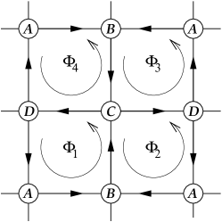
Figure 2: 2$\times$2 four-site square lattice used in the numerical tests. The absolute value of the hopping parameter $t$ is set to 1. $\Phi_{1\cdots 4}$ are the threading fluxes through the four plaquettes.

The on-site energies $\left(E_{A},E_{B},E_{C},E_{D}\right)$ have been set to the values $(-3,0,-3,0)$. This choice results in an insulator with two groups of two entangled bands as shown in Fig. 3. Switching on the fluxes splits the bands along the X–L line, which are otherwise two-fold degenerate. The ${\bf k}$-derivative of Bloch orbitals was computed by the sum-over-states formula Eq. (51). We treated the two lowest bands as filled and we verified that the multi-band Chern number is zero.

Figure 3: Band structure of the square lattice for $\phi=\pi/10$. The flux pattern is $\left(\Phi_{1},\Phi_{2},\Phi_{3},\Phi_{4}\right)=\left(2\phi,-\phi,0,-\phi\right)$, and the on-site energies are $\left(E_{A},E_{B},E_{C},E_{D}\right)=(-3,0,-3,0)$ (see also Fig. 2). The two lower bands are treated as occupied.

We built square finite samples, cut from the bulk, made of $L\times L$ four-site unit cells and having $2L+1$ sites on each edge. Their orbital magnetization (dipole per unit area) $M(L)$ is straightforwardly computed as in Eq. (4). We expect the $L\rightarrow\infty$ asymptotic behavior

$$M(L)=M+a/L+b/L^{2},$$ (52)

where $M$ is the bulk magnetization according to Eq. (48). The terms $a/L$ and $b/L^{2}$ account for edge and corner corrections, respectively.

We performed calculations up to $L=14$ (841 lattice sites). The resulting orbital magnetization as a function of the parameter $\phi$ is shown in Fig. 4. We independently computed the bulk orbital magnetization $M$ from a discretization of the reciprocal-space formula Eq. (48). We get well converged results (to within 0.1%) for a 50$\times$50 ${\bf k}$-point mesh in the full BZ.

Figure 4: Orbital magnetization of the square-lattice model as a function of the parameter $\phi$. The two lower bands are treated as occupied. Open circles: extrapolation from finite-size samples. Solid line: discretized ${\bf k}$-space formula, Eq. (31).

So far, we have studied a model multi-band insulator, having zero Chern number. For this specific case we provided above a solid analytic proof of our reciprocal-space formula, which holds in the thermodynamic limit. Indeed, the numerical results confirm the correctness of the ${\bf k}$-space formula, while also providing some information about actual finite-size effects and numerical convergence.

III.2 Metallic case

In the previous section we addressed the case of a TR-broken multi-band insulator, by treating the two lowest bands as occupied. Here we are going to extend our analysis to the metallic case. We are using the same model Hamiltonian as in the previous section, but we allow the Fermi level to span the energy range roughly from $-$5.45 to 2.45 energy units, namely from the bottom of the lowest band to the top of the highest one. In order to smooth Fermi-surface singularities, and to obtain well converged results, we adopt the simple Fermi-Dirac smearing technique, widely used in first-principle electronic-structure calculations. This amounts to replace, the (integer) Fermi occupation factor $\Theta(\mu-\epsilon_{n{\bf k}})$ with a suitable smooth function $f_{\mu}(\epsilon_{n{\bf k}})$. We therefore replace in Eq. (48):

$$\sum_{n,\epsilon_{n{\bf k}}<\mu}\rightarrow\sum_{n}f_{\mu}(\epsilon_{n{\bf k}}).$$ (53)

Reasoning in terms of a fictitious temperature, one may choose a Fermi-Dirac distribution

$$f_{\mu}(\epsilon)=\frac{1}{1+\exp[(\epsilon-\mu)/\sigma]}.$$ (54)

In all subsequent calculations, we set $\sigma=0.05$ a.u., which provides good convergence.

We compute the orbital magnetization as a function of the chemical potential $\mu$ with $\phi$ fixed at $\pi/3$. Using the same procedure as in the previous section, we compute the orbital magnetization by the means of the heuristic ${\bf k}$-space formula, Eq. (48), and we compare it to the extrapolated value from finite samples, from $L$=8 (289 sites) to $L$=16 (1089 sites). We verified that a ${\bf k}$-point mesh of 100$\times$100 gives well converged results for the bulk formula, Eq. (48).

The orbital magnetization as a function of the chemical potential for $\phi=\pi/3$ is shown in Fig. 5. The resulting values agree to a good level, and provide solid numerical evidence in favor of Eq. (48), whose analytical proof is still lacking. The orbital magnetization initially increases as the filling of the lowest band increases, and rises to a maximum at a $\mu$ value of about $-$4.1. Then, as the filling increases, the first (lowest) band crosses the second band and the orbital magnetization decreases, meaning that the two bands carry opposite-circulating currents giving rise to opposite contributions to the orbital magnetization. The orbital magnetization remains constant when $\mu$ is scanned through the insulating gap. Upon further increase of the chemical potential, the orbital magnetization shows a symmetrical behavior as a function of $\mu$, the two upper bands having equal but opposite dispersion with respect to the two lowest bands (see Fig. 3).

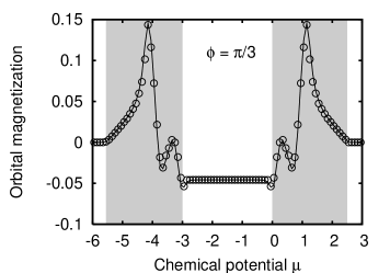
Figure 5: Orbital magnetization of the square-lattice model as a function of the chemical potential $\mu$ for $\phi=\pi/3$. The shaded areas correspond to the two groups of bands. Open circles: extrapolation from finite-size samples. Solid line: discretized ${\bf k}$-space formula, Eq. (48).

III.3 Chern insulating case

In order to check the validity of our heuristic Eq. (48) for a Chern insulator, we switch to the Haldane model HamiltonianHaldane88 that we used in a previous paperThonhauser05 to address the $C=0$ insulating case. In fact, depending on the parameter choice, the Chern number $C$ within the model can be either zero or nonzero (actually, $\pm 1$).

The Haldane model is comprised of a honeycomb lattice with two tight-binding sites per cell with site energies $\pm\Delta$, real first-neighbor hoppings $t_{1}$, and complex second-neighbor hoppings $t_{2}e^{\pm i\varphi}$, as shown in Fig. 6. The resulting Hamiltonian breaks TR symmetry and was proposed (for $C=\pm 1$) as a realization of the quantum Hall effect in the absence of a macroscopic magnetic field. Within this two-band model, one deals with insulators by taking the lowest band as occupied.

In our previous paper Thonhauser05 we restricted ourselves to $C=0$ to demonstrate the validity of Eq. (48), which was also analytically proved. In the present work we address the $C\neq 0$ insulating case, where instead we have no proof of Eq. (48) yet. We are thus performing computer experiments in order to explore uncharted territory.

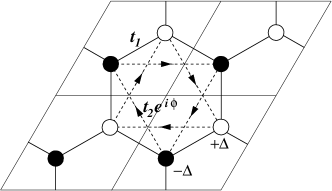
Figure 6: Four unit cells of the Haldane model. Filled (open) circles denote sites with $E_{0}=-\Delta$ ($+\Delta$). Solid lines connecting nearest neighbors indicate a real hopping amplitude $t_{1}$; dashed arrows pointing to a second-neighbor site indicates a complex hopping amplitude $t_{2}e^{i\phi}$. Arrows indicate sign of the phase $\phi$ for second-neighbor hopping.

Following the notation of Ref. Haldane88, , we choose the parameters $\Delta=1$, $t_{1}=1$ and $|t_{2}|=1/3$. As a function of the flux parameter $\phi$, this system undergoes a transition from zero Chern number to $|C|=1$ when $|\sin\phi|>1/\sqrt{3}$.

First we checked the validity of Eq. (48) in the Chern insulating case by treating the lowest band as occupied. We computed the orbital magnetization as a function of $\phi$ by Eq. (48) at a fixed $\mu$ value, and we compared it to the magnetization of finite samples cut from the bulk. For the periodic system, we fix $\mu$ in the middle of the gap; for consistency, the finite-size calculations are performed at the same $\mu$ value, using the Fermi-Dirac distribution of Eq. (54). The finite systems have therefore fractional orbital occupancy and a noninteger number of electrons. The biggest sample size was made up of 20$\times$20 unit cells (800 sites). The comparison between the finite-size extrapolations and the discretized ${\bf k}$-space formula is displayed in Fig. 7. This heuristically demonstrates the validity of our main results, Eqs. (46) and (48), in the Chern-insulating case.

Figure 7: Orbital magnetization of the Haldane model as a function of the parameter $\phi$. The lowest band is treated as occupied. Open circles: extrapolation from finite size samples. Solid line: Eq. (48). The system has non-zero Chern number in the region in between the two vertical lines.

Next, we checked the validity of Eq. (48) for the most general case, following the transition from the metallic phase to the Chern insulating phase as a function of the chemical potential $\mu$. To this aim we keep the model Hamiltonian fixed, choosing $\phi=0.7\pi$; for $\mu$ in the gap this yields a Chern insulator. The behavior of the magnetization while $\mu$ varies from the lowest-band region, to the gap region, and then to the highest-band region is displayed in Fig. 8, as obtained from both the finite-size extrapolations and the discretized ${\bf k}$-space formula. This shows once more the validity of our heuristic formula. Also notice that in the gap region the magnetization is perfectly linear in $\mu$, the slope being determined by the lowest-band Chern number according to Eq. (49).

IV Conclusions

We present here a formalism for the calculation of the orbital magnetization in extended systems with broken TR symmetry, in the case of vanishing (or commensurate) macroscopic $B$ field. This extends our previous work of Ref. Thonhauser05, to the multi-band case, essential for realistic calculations.

First, we consider the case of zero Chern invariant, where we provide an an analytic proof, based upon the Wannier representation. Our main result, Eq. (31), takes the form of a BZ integral of a gauge-invariant quantity, which can easily be computed using reciprocal-space discretization. We provide numerical tests for a two-dimensional model, where our discretized formula is checked against calculations performed for finite samples cut from the bulk, with “open” boundary conditions. Our numerical tests appear to confirm that indeed Eq. (31) is the correct expression for the orbital magnetization in a periodic system.

Second, we propose a heuristic extension of Eq. (31) to the case of non-zero Chern invariant, based on the observation that the integrand in Eq. (31) is gauge invariant, contrary to the analogous electrical case, where only the BZ integral is gauge-invariant, not the integrand.KSV ; rap-a12 On the basis of general considerations (namely, invariance by translation of the energy zero), the minimal modification extending Eq. (31) to the nonzero-Chern-number case yields Eq. (46). Remarkably, Eq. (46) is essentially identical to a recent expression derived by Xiao et al. Xiao05 in the context of a semiclassical approximation. We check the full quantum-mechanical validity of Eq. (46) on a two-dimensional model by means of numerical tests, comparing to finite size calculations as above. The agreement is excellent, thus providing strong support for our formula, well beyond the semiclassical regime, even though we cannot yet provide an analytic proof of it.

Third, since our heuristic Eq. (46) is well-defined for a KS metal, we also check the validity of Eq. (46) using the same two-dimensional model as for the metallic case, this time allowing the chemical potential $\mu$ to be varied through the bands. Once more the agreement is excellent, providing a numerical demonstration of the validity of Eq. (46).

The electrical analogue of the present theory is the modern theory of polarization,KSV ; rap-a12 developed in the 1990s, and valid for insulators only. When comparing that theory with the present one, in the insulating case, there is an important difference which is worth stressing. In the electrical case, the whole electronic contribution to the macroscopic polarization can be expressed in terms of the electric dipoles of the bulk WFs. This has a precise counterpart here, where the local-circulation contribution can in fact be expressed in terms of the magnetic dipoles of the bulk WFs. However, we have shown that in the magnetic case there is an additional “itinerant-circulation” contribution which has no electrical analogue. When analyzing finite samples, the latter contribution appears to be due to chiral currents circulating at the sample boundaries. Nonetheless, one of our major findings is that even this contribution can be expressed as a bulk, boundary-insensitive term.

Both our original expression, Eq. (31), and its heuristic extension, Eq. (46), for the orbital magnetization of a crystalline solid can easily be implemented in existing first-principle electronic structure codes, making available the computation of the orbital magnetization in crystals, at surfaces and in reduced dimensionality solids such as nanowires.

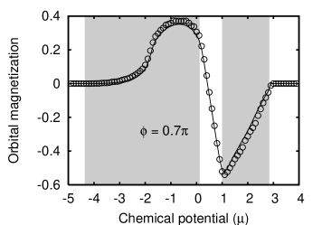
Figure 8: Orbital magnetization of the Haldane model as a function of the chemical potential $\mu$ for $\phi=0.7\pi$. The shaded areas correspond the position of the two bands. Open circles: extrapolation from finite-size samples. Solid line: discretized ${\bf k}$-space formula, Eq. (48).

Appendix A: Finite difference evaluation of the Chern invariant and magnetization

Using the definition of the covariant derivativeSai02 ; Souza04

$$|\widetilde{\partial}_{\alpha}u_{n{\bf k}}\rangle=Q_{\bf k}\,|\partial_{\alpha}u_{n{\bf k}}\rangle,$$ (55)

Eqs. (33-35) can be rewritten as

$$f_{{\bf k},\alpha\beta}=\sum_{n}\langle\widetilde{\partial}_{\alpha}u_{n{\bf k}}|\widetilde{\partial}_{\beta}u_{n{\bf k}}\rangle,$$ (56)

$$g_{{\bf k},\alpha\beta}=\sum_{n}\langle\widetilde{\partial}_{\alpha}u_{n{\bf k}}|H_{\bf k}|\widetilde{\partial}_{\beta}u_{n{\bf k}}\rangle,$$ (57)

$$h_{{\bf k},\alpha\beta}=\sum_{nn^{\prime}}E_{nn^{\prime}{\bf k}}\,\langle\widetilde{\partial}_{\alpha}u_{n^{\prime}{\bf k}}|\widetilde{\partial}_{\beta}u_{n{\bf k}}\rangle.$$ (58)

We assume that the occupied wavefunctions $|u_{n{\bf k}}\rangle$ have been computed on a regular mesh of k-points, and we let ${\bf b}_{1}$, ${\bf b}_{2}$, and ${\bf b}_{3}$ be the primitive reciprocal vectors that define the k-mesh. Then the covariant derivative in mesh direction $i$ can be defined as

$$|\widetilde{\partial}_{i}u_{n{\bf k}}\rangle={\bf b}_{i\alpha}\,|\widetilde{\partial}_{\alpha}u_{n{\bf k}}\rangle$$ (59)

(sum over $\alpha$ implied). Inserting this into Eqs. (56-58) and taking the antisymmetric imaginary part as in Eq. (41), we obtain

$$\tilde{\bf f}_{\bf k}=\frac{1}{v}\,\epsilon_{ijl}\,{\bf b}_{i}\sum_{n}{\rm Im}\langle\widetilde{\partial}_{j}u_{n{\bf k}}|\widetilde{\partial}_{l}u_{n{\bf k}}\rangle,$$ (60)

$$\tilde{\bf g}_{\bf k}=\frac{1}{v}\,\epsilon_{ijl}\,{\bf b}_{i}\sum_{n}{\rm Im}\langle\widetilde{\partial}_{j}u_{n{\bf k}}|H_{\bf k}|\widetilde{\partial}_{l}u_{n{\bf k}}\rangle,$$ (61)

$$\tilde{\bf h}_{\bf k}=\frac{1}{v}\,\epsilon_{ijl}\,{\bf b}_{i}\sum_{nn^{\prime}}E_{nn^{\prime}{\bf k}}\,{\rm Im}\langle\widetilde{\partial}_{j}u_{n^{\prime}{\bf k}}|\widetilde{\partial}_{l}u_{n{\bf k}}\rangle,$$ (62)

where a sum over $ijk$ is implied and $v$ is the volume of the unit cell of the k-space mesh. On this mesh, the BZ integral in Eq. (42) becomes a summation

$${\bf C}=\frac{1}{2\pi}\sum_{\bf k}\epsilon_{ijl}\,{\bf b}_{i}\sum_{n}{\rm Im}\langle\widetilde{\partial}_{j}u_{n{\bf k}}|\widetilde{\partial}_{l}u_{n{\bf k}}\rangle$$ (63)

and similarly for the magnetization in Eq. (43).

The appropriate finite-difference discretization of the covariant derivative in mesh direction $i$ isSai02 ; Souza04

$$|\widetilde{\partial}_{i}u_{n{\bf k}}\rangle=\frac{1}{2}\,\Big{(}\,|\widetilde{u}_{n,{\bf k}+{\bf b}_{i}}\rangle-|\widetilde{u}_{n,{\bf k}-{\bf b}_{i}}\rangle\Big{)}$$ (64)

where $|\widetilde{u}_{n,{\bf k}+{\bf q}}\rangle$ is the “dual” state, constructed as a linear combination of the occupied $|u_{n,{\bf k}+{\bf q}}\rangle$ at neighboring mesh point ${\bf q}$, having the property that $\langle u_{n^{\prime}{\bf k}}|\widetilde{u}_{n,{\bf k}+{\bf q}}\rangle=\delta_{n^{\prime}n}$. This ensures that $\langle u_{n^{\prime}{\bf k}}|\widetilde{\partial}_{i}u_{n{\bf k}}\rangle=0$ consistent with Eq. (55), and is solved by the constructionSai02 ; Souza04

$$|\widetilde{u}_{n,{\bf k}+{\bf q}}\rangle=\sum_{n^{\prime}}\,(S^{-1}_{{\bf k},{\bf k}+{\bf q}})_{n^{\prime}n}\,|u_{n^{\prime},{\bf k}+{\bf q}}\rangle$$ (65)

where

$$(S_{{\bf k},{\bf k}+{\bf q}})_{nn^{\prime}}=\langle u_{n{\bf k}}|u_{n^{\prime},{\bf k}+{\bf q}}\rangle.$$ (66)

Eqs. (60-66) provide the formulas needed to calculate the three gauge-invariant quantities $\tilde{\bf f}_{\bf k}$, $\tilde{\bf g}_{\bf k}$, and $\tilde{\bf h}_{\bf k}$ on each point of the k-mesh. By summing these as in Eq. (63) it is straightforward to obtain $\bf C$, $\widetilde{{\bf M}}_{\rm LC}$, and $\widetilde{{\bf M}}_{\rm IC}$, respectively. Since we have derived this finite-difference representation using gauge-invariant quantities at each step, it is not surprising that we obtain the gauge-invariant contributions $\widetilde{{\bf M}}_{\rm LC}$ and $\widetilde{{\bf M}}_{\rm IC}$, as opposed to the gauge-dependent ${\bf M}_{\rm LC}$ and ${\bf M}_{\rm IC}$, from this approach.

Appendix B: The nonAbelian Berry curvature

It has been noticed in Sec. II.4 that the vector quantity $\tilde{\bf f}_{\bf k}$ is the Berry curvature. From Eqs. (38) and (41), this can be regarded as the trace of the $N_{b}\times N_{b}$ matrix ${\bf F}_{{\bf k}}$ having vector elements

$${\bf F}_{{\bf k},nn^{\prime}} = i\,\langle\partial_{\bf k}u_{n{\bf k}}|\times|\partial_{\bf k}u_{n^{\prime}{\bf k}}\rangle$$ (67)

$$- i\sum_{m}\langle\partial_{\bf k}u_{n{\bf k}}|u_{m{\bf k}}\rangle\times\langle u_{m{\bf k}}|\partial_{\bf k}u_{n^{\prime}{\bf k}}\rangle.$$

This quantity is known within the theory of the geometric phase as the nonAbelian Berry curvature, nonAb and characterizes the evolution of an $N_{b}$-dimensional manifold (here, the states $|u_{n{\bf k}}\rangle$) in a parameter space (here, ${\bf k}$-space). The nonAbelian curvature is gauge-covariant, meaning that if the states are unitarily transformed as

$$|u_{n{\bf k}}\rangle\;\rightarrow\;\sum_{n^{\prime}}U_{nn^{\prime}}({\bf k})|u_{n^{\prime}{\bf k}}\rangle,$$ (68)

then the matrix ${\bf F}_{{\bf k}}$ transforms as

$${\bf F}_{{\bf k},nn^{\prime}}\;\rightarrow\;\sum_{mm^{\prime}}U_{nm}^{\dagger}({\bf k}){\bf F}_{{\bf k},mm^{\prime}}U_{m^{\prime}n^{\prime}}({\bf k}).$$ (69)

This implies that the invariants of the matrix ${\bf F}_{{\bf k}}$, such as its trace $\tilde{\bf f}_{\bf k}$, are gauge-invariant. In fact, as discussed in Sec. II.4, $\tilde{\bf f}_{\bf k}$ behaves like a standard (i.e., Abelian) curvature.

We also notice that the energy matrix $E_{\bf k}$, Eq. (1), is also gauge-covariant in the sense of Eq. (69). It is then easy to verify that the trace (over the band indices) of the matrix product $E_{\bf k}\,{\bf F}_{\bf k}$ is a gauge-invariant quantity. In fact, this trace is identical to $\tilde{\bf h}_{\bf k}$ as defined in Sec. II.4, whose gauge-invariance we proved in a different way. The special $N_{b}=1$ case was previously dealt with in Ref. Thonhauser05, , where the analogue of $\tilde{\bf h}_{\bf k}$ takes the form of the product of energy times curvature, both gauge-invariant quantities. The present finding shows that, in the multi-band case, this must be generalized as the trace of the (matrix) product $E_{\bf k}$ times ${\bf F}_{\bf k}$, both gauge-covariant quantities.

References

- (1) I. Zutic, J. Fabian, and S. Das Sarma, Rev. Mod. Phys. 76, 323 (2004).
- (2) F. Mauri and S. G. Louie, Phys. Rev. Lett. 76, 4246 (1996).
- (3) D. Sebastiani and M. Parrinello, J. Phys. Chem. A 105, 1951 (2001).
- (4) F. Mauri, B. G. Pfrommer, and S. G. Louie, Phys. Rev. Lett. 77, 5300 (1996); C. J. Pickard and F. Mauri, Phys. Rev. Lett. 88, 086403 (2002).
- (5) D. Sebastiani, G. Goward, I. Schnell, and M. Parrinello, Computer Phys. Commun. 147, 707 (2002).
- (6) R. Resta, D. Ceresoli, T. Thonhauser, and D. Vanderbilt, ChemPhysChem 6, 1815 (2005).
- (7) T. Thonhauser, D. Ceresoli, D. Vanderbilt, and R. Resta, Phys. Rev. Lett. 95, 137205 (2005).
- (8) R. D. King-Smith and D. Vanderbilt, Phys. Rev. B 47, 1651 (1993); D. Vanderbilt and R. D. King-Smith, Phys. Rev. B 48, 4442 (1993).
- (9) R. Resta, Rev. Mod. Phys. 66, 899 (1994).
- (10) D. Xiao, J. Shi, and Q. Niu, Phys. Rev. Lett. 95, 137204 (2005).
- (11) F. D. M. Haldane, Phys. Rev. Lett. 61, 2015 (1988).
- (12) Theory of the Inhomogeneous Electron Gas, edited by S. Lundqvist and N. H. March (Plenum, New York, 1983).
- (13) G. Vignale and M. Rasolt, Phys. Rev. B 37, 10685 (1988).
- (14) E. Runge and E. K. U. Gross, Phys. Rev. Lett. 52, 997 (1984).
- (15) S. K. Gosh and A. K. Dhara, Phys. Rev. A 38, 1149 (1988); G. Vignale, Phys. Rev. B 70, 201102(R) (2004).
- (16) K. Ohgushi, S. Murakami, and N. Nagaosa, Phys. Rev. B 62, R6065 (2000).
- (17) T. Jungwirth, Q. Niu, and A. H MacDonald, Phys. Rev. Lett. 88, 207208 (2002).
- (18) S. Murakami, N. Nagaosa, and S.-C. Zhang, Science 301, 1348 (2003).
- (19) Y. Yao, L. Kleinman, A. H. MacDonald, J. Sinova, T. Jungwirth, D.-S. Wang, E. Wang, and Q. Niu, Phys. Rev. Lett. 92, 037204 (2004).
- (20) N. Marzari and D. Vanderbilt, Phys. Rev. B 56, 12847 (1997).
- (21) D. J. Thouless, Topological Quantum Numbers in Nonrelativistic Physics (World Scientific, Singapore, 1998).
- (22) S.F. Boys, Rev. Mod. Phys. 32, 296 (1960); J.M. Foster and S.F. Boys, ibid. 300.
- (23) B. I. Halperin, Phys. Rev. B 25, 2185 (1982).
- (24) D. Yoshioka, The Quantum Hall Effect (Springer, Berlin, 2002), Sec. 3.2.
- (25) D. J. Thouless, M. Kohmoto, M. P. Nightingale, and M. den Nijs, Phys. Rev. Lett. 49, 405 (1982).
- (26) M. Kohmoto, Ann. Phys. 160, 343 (1985).
- (27) Q. Niu, D. J. Thouless, and Y. S. Wu, Phys. Rev. B 31, 3372 (1985).
- (28) G. Sundaram and Q. Niu, Phys. Rev. B 59, 14915 (1999).
- (29) M. V. Berry, Proc. Roy. Soc. Lond. A 392, 45 (1984).
- (30) R. Resta and S. Sorella, Phys. Rev. Lett. 82, 370 (1999).
- (31) R. Resta, Phys. Rev. Lett. 95, 196805 (2005).
- (32) F. D. M. Haldane, Phys. Rev. Lett. 93, 206602 (2004).
- (33) N. Sai, K. M. Rabe, and D. Vanderbilt, Phys. Rev. B 66, 104108 (2002).
- (34) I. Souza, J. Íñiguez and D. Vanderbilt, Phys. Rev. B 69, 085106 (2004).
- (35) S. Baroni, S. de Gironcoli, A. Dal Corso, and P. Giannozzi, Rev. Mod. Phys. 73, 515 (2001).
- (36) A. Bohm, A. Mostafazadeh, H. Koizumi, Q. Niu, and J. Zwanzinger, The Geometric Phase in Quantum Systems (Springer, Berlin, 2003), Ch. 7.