Field Theory Renormalization Group: The Tomonaga-Luttinger Model Revisited

Abstract

We apply field theoretical renormalization group (RG) methods to describe the Tomonaga-Luttinger model as an important test ground to deal with spin-charge separation effects in higher spatial dimensions. We calculate the RG equations for the renormalized forward couplings $g_{2R}$ and $g_{4R}$ up to two-loop order and demonstrate that they don’t flow in the vicinities of the Fermi points (FPs). We solve the Callan-Symanzik equation for $G_{\left(a\right)R}$ in the vicinities of the FPs. We calculate the related spectral function and the momentum distribution function at $p=k_{F},p_{0}=\omega$. We compute the renormalized one-particle irreducible function $\Gamma_{\left(+\right)R}^{\left(2\right)}\left(p,p_{0}=0;\Lambda\right)$ and show it carries important spin-charge separation effects in agreement with well known results. Finally we discuss the implementation of the RG scheme taking into account the important simplifications produced by the Ward identities.

1 Introduction

The discovery of high-temperature superconductors and other related oxide based materials have attracted a lot of attention regarding the unique properties of low dimensional solids. The simplest and more notorious representation of a one-dimensional (1d) conductor is the the so-called Tomonaga-Luttinger (TL) model[1]. That model essentially describes 1d electrons in the vicinity of their right and left Fermi points interacting with each other by means of forward scattering processes. Due to the special equivalence relations between bosons and fermions and left and right charge conservation laws the TL model can be solved exactly by either bosonization[2] or, making full use of the Ward identities, by quantum field theory methods[3].

The one-particle Green’s function for the TL model can also be calculated exactly by those methods. However such a direct solution is provided only in coordinate space. To obtain the associated spectral function which determines the photoemission and the inverse photoemission spectra one needs to evaluate an intricate double Fourier transform and perform numerical approximations[4].

Bosonization methods are hard to implement in higher dimensions[5]. In addition, those Ward identities simplifications are inherent to 1d and to the exact number conservation of right (+) and left (-) particles. As a result to deal with strongly correlated fermions in two or more spatial dimensions one generally resorts to other schemes. One of those alternative approaches is the renormalization group (RG) method. RG methods were used with success to predict the various instabilities of the 1d electron gas as a function of the existing coupling parameters[6]. The RG flows of the renormalized couplings are also in agreement with the bosonization solutions in several related problems. Despite that the RG method is not frequently used to perform a direct calculation of the single-particle Green’s function and its associated spectral function[7, 8]. Since in the TL model there are only low-energy bosonic spin and charge collective modes it is not clear that the right physics will emerge out of approximate fermionic RG schemes. Besides, it is also fair to say that RG methods have not yet been proved capable of dealing, in full force, with spin-charge separation effects. Within the g-ology framework the role of the forward coupling $g_{4}$ has not been fully explored in the RG context so far. One should therefore try to establish how to deal with spin-charge effects in well known grounds, such as the TL model, before implementing RG methods in more difficult problems such as spin-charge separated states in higher spatial dimensions.

In this work we apply the field theoretical RG method[9] to describe the TL model in detail. This work is not intended to review exhaustively all the different RG applications for the TLM. We refer the reader to several authoritative review articles for that purpose[10]. Rather we concentrate here uniquely on the field theoretical RG description of the TLM. Using this scheme we derive the flow equations for the forward couplings $g_{2R}$ and $g_{4R}$ up to two-loop order. In calculating the respective renormalized one-particle irreducible functions $\Gamma_{2R}^{(4)}$ and $\Gamma_{4R}^{(4)}$ we show that non-parquet vertex contributions are the only source of logarithmic divergences in our perturbative calculations. Taking into account the self-energy corrections calculated earlier we demonstrate that, in two-loop order, the non-flow condition for $g_{2R}$ and $g_{4R}$ is assured by the exact cancelation produced by the contributions originated by the anomalous dimension and by the counterterms added to our renormalized TL Lagrangian. Based on our perturbative RG results we construct and solve the Callan-Symanzik equation for the renormalized one-particle Green’s function $G_{R}$ at the Fermi points. We show that it correctly possesses a branch cut structure due to its non trivial anomalous dimension. Using $G_{R}$ we derive the spectral function and the momentum distribution function at the Fermi points. Our results are in agreement with earlier bosonization work[4] as well as more recent RG estimates[9]. Using a momentum RG scale parameter we use perturbation theory to derive $\Gamma_{R}^{(2)}=G_{R}^{-1}$ at the Fermi energy $p_{0}=0$ and in the vicinity of $p=\pm k_{F}$. One important feature emerges naturally from our result. There are now two emergent characteristic velocities which we relate immediately to the spin-charge separation effects. Moreover, the general form of the resulting $\Gamma_{R}^{(2)}$ is in qualitative agreement with the Dzyaloshinskii and Larkin’s Ward identity solution(DL)[3]. Our estimates are entirely perturbative since at that stage we only consider contributions up to two-loop order. To go beyond perturbation theory we relate the effective two-particle propagators $D_{+-}$ and $D_{++}$, introduced earlier by DL, to $\Gamma_{2R}^{(4)}$ and $\Gamma_{4R}^{(4)}$ and show how to implement the regularization, up to infinite order, of all the divergences which are originated in the perturbation series for these two one-particle irreducible functions.

Recently new versions of the functional RG containing both fermionic and auxiliary bosonic fields have been developed with success[14, 15]. In one of those[14], the Ward identities are also used to truncate the vertex functions hierarchical equations and as a result they are able to reproduce the correct TL spectral function at the Fermi points for the case in which $g{}_{4}=0$.

2 The TL Lagrangian Model

Following the so-called g-ology convention the renormalized TL fermionic lagrangian is given by

$$L_{TL}=\sum_{p,a=\pm,\sigma}(1+\Delta Z)\psi_{R(a)\sigma}^{\dagger}(p,t)(i\partial_{t}-v_{F}(\left|p\right|-k_{F}))\psi_{R(a)\sigma}(p,t)$$

$$-\sum_{p_{1}p_{2}p_{3}\atop\sigma_{1},\sigma_{2}}(g_{2R}+\Delta g_{2R})\psi_{R(+)\sigma_{1}}^{\dagger}(p_{3},t)\psi_{R(-)\sigma_{2}}^{\dagger}(p_{1}+p_{2}-p_{3},t)\psi_{R(-)\sigma_{2}}(p_{2},t)\psi_{R(+)\sigma_{1}}(p_{1},t)$$

$$-\frac{1}{2}\sum_{p_{1}p_{2}p_{3}\atop\sigma_{1},\sigma_{2},a}(g_{4R}+\Delta g_{4R})\psi_{R(a)\sigma_{1}}^{\dagger}(p_{3},t)\psi_{R(a)\sigma_{2}}^{\dagger}(p_{1}+p_{2}-p_{3},t)\psi_{R(a)\sigma_{2}}(p_{2},t)\psi_{R(a)\sigma_{1}}(p_{1},t),$$ (1)

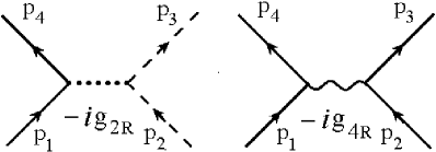
Figure 1: The direct renormalized couplings.

where the momentum $p$ is restricted to the interval $-\lambda\leq\left|p\right|-k_{F}\leq\lambda$ in the vicinities of the right and left Fermi points and $\Delta Z=Z-1$. In Figure 1 we display the direct couplings $g_{2R}$ and $g_{4R}$. For practical purposes we can also take the limit $\lambda\rightarrow\infty$. We assume beforehand that neither the Fermi velocity nor the Fermi momentum are renormalized by interactions. The quasiparticle weight Z is nullified by interactions at the Fermi points since there are no stable quasiparticles in the TL regime but we assume tactically that we don’t know this a priori. In general Z is the multiplicative factor which relate the bare and the renormalized fermion fields to each other. The counterterms associated with the contributions from $\Delta g_{2R}$ and $\Delta g_{4R}$ are included to regularize the logarithmic divergences which arise in perturbation theory.

The corresponding right and left non-interacting Green’s functions of this model are simply

$$iG_{\left(+\right)}^{\left(0\right)}\left(p,p_{0}\right)=i\left[\frac{\theta\left(p-k_{F}\right)}{p_{0}-v_{F}\left(p-k_{F}\right)+i\delta}+\frac{\theta\left(k_{F}-p\right)}{p_{0}-v_{F}\left(p-k_{F}\right)-i\delta}\right]$$ (2)

and

$$iG_{\left(-\right)}^{\left(0\right)}\left(p,p_{0}\right)=i\left[\frac{\theta\left(-\left(p+k_{F}\right)\right)}{p_{0}+v_{F}\left(p+k_{F}\right)+i\delta}+\frac{\theta\left(\left(p+k_{F}\right)\right)}{p_{0}+v_{F}\left(p+k_{F}\right)-i\delta}\right]$$ (3)

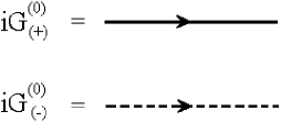
Figure 2: The non-interacting Green’s functions.

Using the appropriate Feynman rules for $L_{TL}$ we can now proceed with the perturbative calculations of the one-particle irreducible functions $\Gamma_{2R}^{\left(4\right)}$, $\Gamma_{4R}^{\left(4\right)}$ and $\Gamma_{2R}^{\left(2\right)}$. In general, following the renormalization theory, we can relate those functions at the Fermi points to observable physical quantities.

Due to the fact that only forward scattering processes are accounted for in $L_{TL}$ the right $\left(+\right)$ and left $\left(-\right)$ lines never mix in a single loop. As a result in this way no divergence arises from non-interacting particle-hole loop diagrams. Taking into account the spin summation factors we find instead

$$\Pi_{\left(+\right)}^{\left(0\right)}\left(q,q_{0}\right)=\frac{iq}{\pi}\left[\frac{\theta\left(q\right)}{q_{0}-v_{F}q+i\delta}+\frac{\theta\left(-q\right)}{q_{0}-v_{F}q-i\delta}\right]$$ (4)

and

$$\Pi_{\left(-\right)}^{\left(0\right)}\left(q,q_{0}\right)=-\frac{iq}{\pi}\left[\frac{\theta\left(-q\right)}{q_{0}+v_{F}q+i\delta}+\frac{\theta\left(q\right)}{q_{0}+v_{F}q-i\delta}\right]$$ (5)

These $\Pi^{\left(0\right)}$’s reduce simply to $-i/\pi v_{F}$ at the Fermi points if we take the limits $q_{0}\rightarrow 0$ and $q\rightarrow 0$.

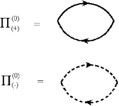
Figure 3: The non-interacting particle-hole bubbles.

Another important feature due to the neglect of backscattering processes is that the symmetrized sums of all diagrams containing closed loops with more than two fermion lines vanish exactly[3]. Thanks to this important simplification there are only divergent diagrams in the perturbative series expansions for both $\Gamma_{2R}^{\left(4\right)}$ and $\Gamma_{4R}^{\left(4\right)}$ in two-loop order. Those divergences, which are precisely the object of attention of renormalization theory, are cancelled out exactly by the counterterms added to the Lagrangian model. However at this order of perturbation theory we are also obliged to take into account self-energy corrections. Therefore before discussing the RG flow of the renormalized couplings we apply the RG method for the calculation of the self-energy $\Sigma_{R\left(+\right)}$.

3 One-Particle Irreducible Function $\Gamma_{2R}^{\left(2\right)}$ up to Two-Loop Order

Computing diagrammatically the self-energy $\Sigma_{R\left(+\right)}\left(p,p_{0}\right)$ for the TL model up to two-loop order, we find:

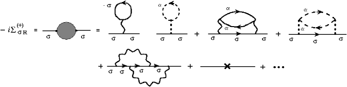
Figure 4: The self-energy $\Sigma_{R(+)\sigma}$.

Evaluating these diagrams we obtain

$$\Sigma_{R\left(+\right)}\left(p,p_{0}\right)=\Sigma_{R\left(+\right)}^{\left(a\right)}\left(p,p_{0}\right)+\Sigma_{R\left(+\right)}^{\left(b\right)}\left(p,p_{0}\right)+\Sigma_{R\left(+\right)}^{\left(c\right)}\left(p,p_{0}\right),$$ (6)

where

$$\Sigma_{R\left(+\right)}^{\left(a\right)}\left(p,p_{0}\right)=\frac{\overline{g}_{2R}\Omega}{2\pi}+\frac{\overline{g}_{4R}\Omega}{4\pi}+\left(\frac{\overline{g}_{4R}}{2\pi\sqrt{2}}\right)^{2}\left(v_{F}\left(p-k_{F}\right)\right)^{2}G_{\left(+\right)}^{\left(0\right)}\left(p,p_{0}\right),$$ (7)

$$\Sigma_{R\left(+\right)}^{\left(b\right)}\left(p,p_{0}\right) = -\Delta Z\left(p_{0}-v_{F}\left(p-k_{F}\right)\right)$$ (8)

and

$$\Sigma_{R\left(+\right)}^{\left(c\right)}\left(p,p_{0}\right)=-\left(\frac{\overline{g}_{2R}}{2\pi\sqrt{2}}\right)^{2}\left(p_{0}-v_{F}\left(p-k_{F}\right)\right)\left\{\ln\left(\frac{\Omega-v_{F}\left|\Delta p\right|+p_{0}-i\delta}{v_{F}\left|\Delta p\right|+p_{0}-i\delta}\right)\right.$$

$$\left.+\ln\left(\frac{\Omega-v_{F}\left|\Delta p\right|+p_{0}-i\delta}{v_{F}\left|\Delta p\right|+p_{0}-i\delta}\right)\right\}$$ (9)

where $\Delta p=p-k_{F}$, $\overline{g}_{iR}=\overline{g}_{iR}/v_{F}$ and $\Omega=2v_{F}\lambda$.

Having established what $\Sigma_{R\left(+\right)}$ is we move on to calculate the related one-particle Green’s function $G_{\left(+\right)R}=\left(\Gamma_{R\left(+\right)}^{\left(2\right)}\right)^{-1}$ where

$$\Gamma_{R\left(+\right)}^{\left(2\right)}\left(p,p_{0}\right)=p_{0}-v_{F}\left(p-k_{F}\right)-\Sigma_{R\left(+\right)}\left(p,p_{0}\right)$$ (10)

To determine $\Delta Z\left(\omega\right)$ we define $\Gamma_{R\left(+\right)}^{\left(2\right)}$ such that, at the RG scale $p_{0}=\omega$, and at the Fermi point $\Delta p=0$, $\Gamma_{R\left(+\right)}^{\left(2\right)}\left(p=k_{F},p_{0}=\omega;\omega\right)=\omega$. Using our two-loop results we get

$$Z\left(\omega\right)=1-\left(\frac{\overline{g}_{2R}}{2\pi}\right)^{2}\ln\left(\frac{\Omega}{\omega}\right)$$ (11)

Notice that the quasiparticle weight $Z\left(\omega\right)$ satisfies the RG equation

$$\omega\frac{d\ln Z\left(\omega\right)}{d\omega}=\gamma,$$ (12)

where $\gamma$ is the anomalous dimension given by

$$\gamma=\left(\frac{\overline{g}_{2R}}{2\pi}\right)^{2}$$ (13)

In view of this $Z\left(\omega\right)$ scales simply with the RG parameter as

$$Z\left(\omega\right)=\left(\frac{\omega}{\Omega}\right)^{\gamma},$$ (14)

and since $\gamma\geq 0$ for non-zero forward coupling $Z\left(\omega\right)$ is nullified at the FP when $\omega\rightarrow 0$ in agreement with the fact that there are no well defined quasiparticles in the TL state. This result was obtained earlier in Refs. [10, 11].

4 Flow Equations for the Renormalized Couplings

Following the renormalization theory we can relate the physical couplings $g_{2R}$ and $g_{4R}$ to the-particle irreducible functions $\Gamma_{2R}^{\left(4\right)}$ and $\Gamma_{4R}^{\left(4\right)}$ at the Fermi points. In this way for the external momenta $p_{1}=p_{3}=k_{F}$, $p_{2}=-k_{F}$ and $p_{10}=p_{20}=p_{30}=\omega/2\approx 0$ we define

$$\Gamma_{2R}^{\left(4\right)}\left(p_{1}=k_{F},p_{2}=-k_{F};p_{1}+p_{2}-p_{3}=-k_{F},p_{3}=k_{F};p_{10}=p_{20}=p_{30}=\omega/2;\omega\right)=-ig_{2R}\left(\omega\right)$$ (15)

and similarly, for $p_{1}=p_{3}=p_{2}=k_{F}$ and $p_{10}=p_{20}=p_{30}=\omega/2$,

$$\Gamma_{4R}^{\left(4\right)}\left(p_{1}=k_{F},p_{2}=k_{F};p_{1}+p_{2}-p_{3}=k_{F},p_{3}=k_{F};p_{10}=p_{20}=p_{30}=\omega/2;\omega\right)=-ig_{4R}\left(\omega\right)$$ (16)

Using standard diagrammatic analysis as shown in the Figure 5 we have at the vicinity of the Fermi point

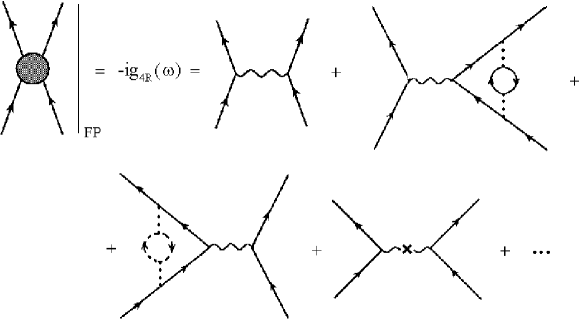
Figure 5: The $g_{4R}$ channel.

$$\Gamma_{4R}^{\left(4\right)}=-ig_{4R}\left(\omega\right)-i\frac{g_{4R}\left(\omega\right)\overline{g}_{2R}^{2}\left(\omega\right)}{2\pi^{2}}\ln\left(\frac{\Omega}{\omega}\right)-i\Delta g_{4R}\left(\omega\right)+...$$ (17)

To be consistent with the definition given above in eqn.16 we then set

$$\Delta g_{4R}\left(\omega\right)=-\frac{g_{4R}\left(\omega\right)\overline{g}_{2R}^{2}\left(\omega\right)}{2\pi^{2}}\ln\left(\frac{\Omega}{\omega}\right)$$ (18)

We display the diagrams for $\Gamma_{2R}^{(4)}|_{FP}$ in Figure 6. Following the same strategy as before we indicate in Figure 7 how to proceed with the calculation of the counterterm $-i\Delta g_{2R}(\omega)$.

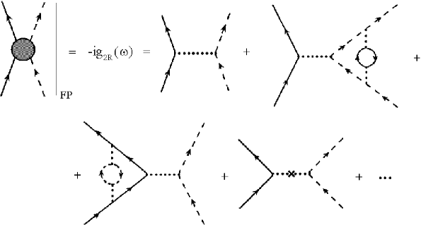
Figure 6: The $g_{2R}$ channel.

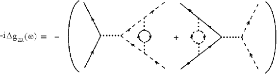
Figure 7: The counterterm $-i\Delta g_{2R}(\omega)$.

From RG theory we know that the bare and renormalized couplings are related to each other by

$$g_{iB}=Z^{-2}\left(\omega\right)\left(g_{iR}+\Delta g_{iR}\right)$$ (19)

Since the bare couplings are independent of the RG scale $\omega$ they satisfy automatically the RG conditions

$$\omega\frac{dg_{2B}}{d\omega}=\omega\frac{dg_{2B}}{d\omega}=0$$ (20)

The flow equations for the corresponding renormalized couplings follow from these conditions. We find immediately that

$$\beta_{i}(\omega)=\omega\frac{dg_{iR}}{d\omega}=2\gamma g_{iR}-\omega\frac{d\Delta g_{iR}}{d\omega}$$ (21)

Using our perturbative results for $\gamma$, $\Delta g_{2R}$ and $\Delta g_{4R}$ we then get that these flow equations are exactly nullified for the TL liquid:

$$\beta_{2}(\omega)=\omega\frac{dg_{2R}}{d\omega}=\beta_{4}(\omega)=\omega\frac{dg_{4R}}{d\omega}=0$$ (22)

A rigorous mathematical proof of the vanishing of the beta functions in all orders of perturbation theory in the TLM is given in Ref. [13].

5 RG Calculation of the One-Particle Green’s Function at the Fermi Points

As we saw in the previous section the TL liquid is characterized by the non-flow of the renormalized forward couplings. This simplifies the RG approach to this problem. In this scheme we relate, quite generically, the renormalized Green’s function $G_{R}$ to its bare analogue $G_{B}$ by

$$G_{\left(a\right)R}\left(p,p_{0};g_{2R};g_{4R};\omega\right)=Z^{-1}\left(\omega\right)G_{\left(a\right)B}\left(p,p_{0};g_{2B};g_{4B}\right)$$ (23)

Since $G_{B}$ is independent of the RG scale $\omega$ we derive the Callan-Symanzik equation (CZE)[16] differentiating $G_{\left(a\right)B}$ with respect to $\omega$. Taking into account that the $g_{iR}$’s don’t flow , in the vicinity of the Fermi points, for $p=\pm k_{F}$, the CZE reduces to

$$\left(\omega\frac{\partial}{\partial\omega}+\gamma\right)G_{\left(a\right)R}\left(p=\pm k_{F},p_{0};\omega\right)=0$$ (24)

Since $G_{\left(a\right)R}$ has ordinary dimension of $\left(energy\right)^{-1}$, on dimensional grounds we have that

$$\left(\omega\frac{\partial}{\partial\omega}+p_{0}\frac{\partial}{\partial p_{0}}\right)G_{\left(a\right)R}\left(p=\pm k_{F},p_{0};\omega\right)=-G_{\left(a\right)R}\left(p=\pm k_{F},p_{0};\omega\right)$$ (25)

We can use this to rewrite the CZE in the form

$$\left(p_{0}\frac{\partial}{\partial p_{0}}+1-\gamma\right)G_{\left(a\right)R}\left(p=\pm k_{F},p_{0};\omega\right)=0$$ (26)

Considering that the anomalous dimension $\gamma$ is constant, this equation can be easily integrated to give

$$G_{\left(a\right)R}\left(p=\pm k_{F},p_{0};\omega\right)=\frac{1}{\omega}\left(\frac{\omega}{p_{0}+i\delta}\right)^{1-\gamma}$$ (27)

which has indeed a branch cut structure as opposed to the simple pole nature, typical of the Fermi liquid one-particle Green’s function. Consequently, for $p_{0}\leq 0$, at the Fermi points,

$$G_{\left(a\right)R}\left(p=\pm k_{F},p_{0};\omega\right)=-\frac{1}{\omega}\left(\frac{\omega}{\left|p_{0}\right|}\right)^{1-\gamma}\left(\cos\pi\gamma+i\sin\pi\gamma\right)$$ (28)

It follows from this that the spectral function $A_{\left(a\right)R}\left(p=\pm k_{F},p_{0};\omega\right)$ reduces to

$$A_{\left(a\right)R}\left(p=\pm k_{F},p_{0};\omega\right)=\theta\left(-p_{0}\right)\left(\frac{\left|p_{0}\right|}{\omega}\right)^{\gamma}\frac{\sin\pi\gamma}{\left|p_{0}\right|}$$ (29)

This result is in agreement with earlier RG estimates of Kopietz and coworkers[8]. To calculate next the momentum distribution function $n\left(p=\pm k_{F}\right)$ at the FPs, it suffices to integrate $A_{\left(a\right)R}$ over an energy interval of width $2\omega$ around $p_{0}=0$. We find

$$n\left(p=\pm k_{F}\right)=\frac{\sin\pi\gamma}{2\pi\gamma}$$ (30)

which reduces to $n\left(\pm k_{F}\right)=1/2$ in the limit $\gamma\rightarrow 0$.

Let us now consider the alternative limit $p_{0}=0$ and $\Delta p=\Lambda\approx 0$ where the parameter $\Lambda$ is now our RG momentum scale which will be used to take the physical system towards the FPs. If we repeat our RG analysis for $\Gamma_{iR}^{\left(4\right)}$ making use of such RG scale we find at the FPs

$$\Delta g_{iR}\left(\omega\right)=-\frac{g_{iR}\left(\omega\right)\overline{g}_{2R}^{2}\left(\omega\right)}{2\pi^{2}}\ln\left(\frac{2\lambda}{\Lambda}\right)$$ (31)

Since the forward couplings don’t flow in the TL we can determine the corresponding $Z\left(\Lambda\right)$ taking into account that we must have as before

$$2\gamma_{\Lambda}g_{iR}=\Lambda\frac{d\Delta g_{iR}}{d\Lambda}=\frac{g_{iR}\left(\omega\right)\overline{g}_{2R}^{2}\left(\omega\right)}{2\pi^{2}}$$ (32)

Consequently,

$$\Lambda\frac{d\ln Z\left(\Lambda\right)}{d\Lambda}=\gamma_{\Lambda}=\gamma$$ (33)

and again we have that

$$Z\left(\Lambda\right)=Z\left(2\lambda\right)\left(\frac{\Lambda}{2\lambda}\right)^{\gamma}\rightarrow 0$$ (34)

as $\Lambda\rightarrow 0$ for $\gamma>0$, which is consistent with the fact that there are no quasiparticles at the FPs.

Invoking once again the RG condition between the bare and renormalized $\Gamma_{\left(+\right)}^{\left(2\right)}$ ’s we write

$$\Gamma_{\left(+\right)R}^{\left(2\right)}\left(p,p_{0}=0;\Lambda\right)=Z\left(\Lambda\right)\Gamma_{\left(+\right)B}^{\left(2\right)}\left(p,p_{0}=0\right)$$ (35)

In the weak coupling limit in a regime consistent with our perturbative two-loop results $Z\left(\Lambda\right)$ reduces to

$$Z\left(\Lambda\right)=1+\gamma\ln\left(\frac{\Lambda}{2\lambda}\right)+...$$ (36)

Combining this with our earlier results produces

$$\Gamma_{\left(+\right)B}^{\left(2\right)}\left(p,p_{0}=0\right)=-v_{F}\Delta p\left[1+\left(\frac{\overline{g}_{2R}}{2\pi}\right)^{2}\ln\left(\frac{2\lambda}{\Delta p}\right)-\left(\frac{\overline{g}_{4R}}{2\pi\sqrt{2}}\right)^{2}\right]$$ (37)

Consequently in the vicinities of the FPs

$$\Gamma_{\left(+\right)R}^{\left(2\right)}\left(p,p_{0}=0;\Lambda\right)=-\frac{u_{c}u_{s}\Delta p}{v_{F}}\left[1+\left(\frac{g_{2R}}{2\pi\sqrt{u_{c}u_{s}}}\right)^{2}\ln\left(\frac{\Lambda}{\Delta p}\right)\right],$$ (38)

with

$$u_{c}=v_{F}\left(1+\frac{|\overline{g}_{4R}|}{2\pi\sqrt{2}}\right)$$ (39)

and

$$u_{s}=v_{F}\left(1-\frac{|\overline{g}_{4R}|}{2\pi\sqrt{2}}\right)$$ (40)

The presence of two different velocities violates the single-pole character of the one-particle Green’s function and it is directly related to the spin-charge separation which takes place in the TLM[17]. This spin-charge separation is a feature which emerges naturally from our perturbative RG analysis. Notice that up to order $O(\overline{g}_{2R}^{2})$, in the weak coupling limit, $v_{F}\approx\sqrt{u_{c}u_{s}}$ and $\Gamma_{\left(+\right)R}^{\left(2\right)}$ reduces to

$$\Gamma_{\left(+\right)R}^{\left(2\right)}\left(p,p_{0}=0;\Lambda\right)\approx-\left(u_{c}\Delta p\right)^{\frac{1}{2}}\left(u_{s}\Delta p\right)^{\frac{1}{2}}\left(\frac{\Lambda}{\Delta p}\right)^{\gamma}$$ (41)

which is in qualitative agreement with well-known results[18]. However, our estimates for $u_{c}$ and $u_{s}$ are only valid up to two-loop order. For this reason they cannot be identical to the velocities obtained from the solutions of Schwinger-Dyson equations which include contributions up to infinite order[3].

6 Ward Identities

As demonstrated by Dzyaloshinskii and Larkin[3] the use of Ward identities greatly simplifies the analysis of the TL model. Making use of these identities and taking into account the simplifications produced by the cancelation of the symmetrized sum of all diagrams containing closed loops with more than two fermion lines we are naturally led, following DL, to introduce two interactions propagators $D_{++}$ and $D_{+-}$. These two propagators can be used to describe the effective two-particle interactions in the TLM. $D_{++}$ and $D_{+-}$ are finite at the FPs and do not need to undergo any regularization procedure. In contrast with that, as we discussed in section 4, the one-particle irreducible functions $\Gamma_{2R}^{\left(4\right)}$ and $\Gamma_{4R}^{\left(4\right)}$ produce non-parquet vertex contributions which need to be regularized order by order in perturbation series. Therefore to relate the DL interaction propagators back to the corresponding one-particle irreducible functions we must include appropriate vertex functions. Considering these feature we can readily extend our perturbative results writing the exact one-particle irreducible functions $\Gamma_{2R}^{\left(4\right)}$ and $\Gamma_{4R}^{\left(4\right)}$ in the form

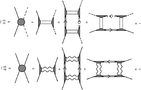
Figure 8: The exact one-particle irreducible functions $\Gamma_{2R}^{(4)}$ and $\Gamma_{4R}^{(4)}$.

$$\Gamma_{2R}^{(4)}\left(p_{1},p_{2},p_{1}+p_{2}-p_{3},p_{3}\right)= \Gamma_{+}^{R}(p_{3},p_{1},p_{3}-p_{1})iD_{+-}\left(p_{1}-p_{3}\right)$$ (42)

$$.\Gamma_{-}^{R}\left(p_{1}+p_{2}-p_{3},p_{3},p_{1}-p_{3}\right)$$

and

$$\Gamma_{4R}^{(4)}\left(p_{1},p_{2},p_{1}+p_{2}-p_{3},p_{3}\right)= \Gamma_{+}^{R}(p_{1},p_{3},p_{3}-p_{1})iD_{++}\left(p_{1}-p_{3}\right)$$ (43)

$$.\Gamma_{+}^{R}\left(p_{1}+p_{2}-p_{3},p_{2},p_{1}-p_{3}\right)$$

These $\Gamma_{iR}^{(4)}$’s are represented diagrammatically in Figure 8. Thanks to the already mentioned simplification inherent to the TLM, the propagators $D_{+-}$ and $D_{++}$ are determined exactly by solving the Schwinger-Dyson equations indicated in Figures 9 and 10. Solving these SDE’s for $D_{++}$ and $D_{+-}$, diagrammatically, we arrive immediately at the DL results for the charge and spin velocities, namely, $u_{c}=v_{F}\sqrt{(1+\overline{g}_{4R}/\pi)^{2}-(\overline{g}_{2R}/\pi)^{2}}$ and $u_{s}=v_{F}$.

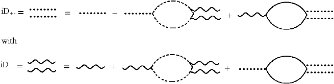
Figure 9: The exact interaction propagators $iD_{+-}$ and $iD_{--}$.

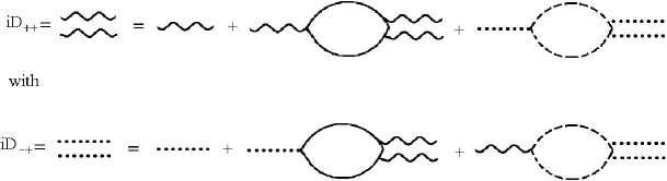
Figure 10: The propagators $iD_{++}$ and $iD_{-+}$.

Since the interaction propagators are independent of renormalization parameters they are RG invariants. In contrast the vertex functions $\Gamma$’s produce logarithmic singularities which need to be cancelled out by appropriate counterterms. As we showed before, in the RG framework, we solve this problem either by relating the bare and renormalized vertices to each other through relations of the type

$$\Gamma_{a}^{R}=Z_{2}\Gamma_{a}^{B}=\left(1+\Delta Z_{2}\right)\Gamma_{a}^{B}$$ (44)

with $a=+,-$, or by constructing the necessary counterterm directly, order by order in perturbation theory. Following this latter route, up to two-loop order the renormalized vertex function $\Gamma_{a}^{R}$ is determined by the diagrams shown in Figure (11).

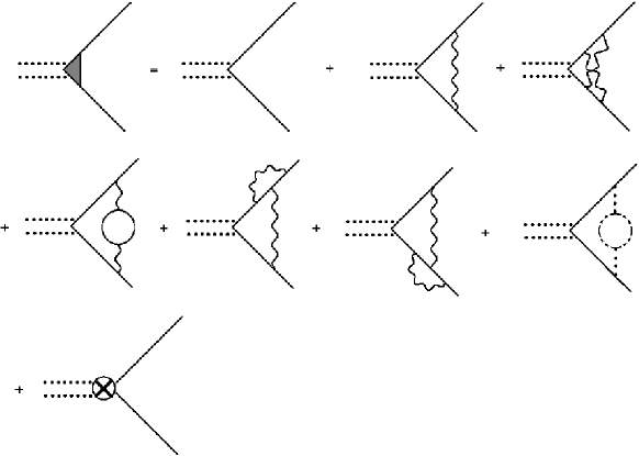
Figure 11: The Renormalized vertex function $\Gamma_{+}^{R}$.

If we define $\Gamma_{a}^{R}$ such that $\left.\Gamma_{a}^{R}\right|_{FP}=1$ it then follows that the vertex counterterm diagram which appears in Figure (12) is determined exactly by this condition.

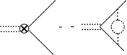
Figure 12: The vertex function counterterm $\Delta\Gamma_{+}^{R}$.

This gives

$$\left.\Delta\Gamma_{+}^{R}\right|_{FP}=-\left(\frac{\overline{g}_{2R}}{2\pi}\right)^{2}\ln\left(\frac{\Omega}{\omega}\right)=\Delta Z$$ (45)

It follows from this that the vertex renormalization constant $Z_{2}$ must be identical to the quasiparticle weight:

$$Z_{2}=Z$$ (46)

Such an equivalence between the vertex renormalization constant $Z_{2}$ and the quasiparticle amplitude $Z$ was also pointed out in Ref. [12]. In fact, since the Ward identity(WI) is preserved by the renormalization process, this result emerges naturally from the WI itself. As a consequence of this simplification, at the FPs, the renormalized one-particle irreducible functions $\Gamma_{2R}^{\left(4\right)}$ and $\Gamma_{4R}^{\left(4\right)}$ reduce simply to the interaction propagators $iD_{+-}$ and $iD_{++}$ respectively, which by being RG invariants, produce vanishing beta functions to all orders in perturbation theory in agreement with the rigorous analysis of Ref. [13].

7 Conclusion

We implement the field theoretical RG method in the presence of spin-charge separation effects in one spatial dimension. We take the Tomonaga-Luttinger model as our reference test ground in dealing with future higher dimensional problems. As is well known trhe TLM was solved by bosonization and by quantum field theoretical methods which take into explicit account the simplifications produced by the Ward identities. Unfortunately those simplifications are inherent to one dimension and contrary to the RG scheme both methods are difficult to implement in more general situations.

Using our RG method we calculate the self-energy up to two-loop order. From it we find a non-zero anomalous dimension and a quasiparticle weight which is nullified at the Fermi points. We compute the RG equations for the renormalized coupling constants $g{}_{2R}$ and $g{}_{4R}$, up to two-loop order, and demonstrate that they don’t flow in the vicinities of the FPs. We derive the Callan-Symanzik equation for the one-particle Green’s function at $p=k_{F},p_{0}=\omega$. The CSE is easily integrated producing an expected branch cut structure in $G_{\left(a\right)R}$. Using this we derive the spectral function and the momentum distribution function at $p=k_{F}$. We calculate the one-particle irreducible function $\Gamma_{\left(+\right)R}^{\left(2\right)}\left(p,p_{0}=0;\Lambda\right)$ taking into explicit account spin-charge separation effects in the weak coupling regime. Our results are in qualitative agreement with the other approaches. Finally we discuss the inclusion of the Ward identities in the RG scheme. We show that their present forms are preserved upon the renormalization and thanks to them the one-particle irreducible functions in the vicinities of the FPs reduce to interaction propagators which can be solved exactly by appropriate Schwinger-Dyson equations. To conclude we add that some of the material discussed in this paper have appeared before in the literature in one form or another. We tried to relate, whenever possible, our results to some of those works. By presenting them here in a field theoretical self-contained form we hope to bring new insights concerning the RG applications with both spin-charge separation effects and Ward identities in more general problems.

Acknowledgements- I wish to acknowledge the discussions and help I had from Eberth Correa and Hermann Freire in the preparation of this paper. This work was financially supported by FINEP and the Min. of Science and Tecnology from Brazil .

References

- [1] Tomonaga S, Prog. Theor. Phys. 5, 544 (1950)
- [2] Mattis D C and Lieb E H, J.Math. Phys. 6, 304 (1965)
- [3] Dzyaloshinskii I E and Larkin A I, Sov.Phys.-JETP 38, 202 (1974)
- [4] Meden V and Schönhammer K, Phys.Rev.B 46, 15753 (1992); Voit J, Phys.Rev.B 47, 6740 (1993)
- [5] Haldane F D, in Proceedings of the International School of Physics “Enrico Fermi”, eds Broglia R A and Schrieffer J R, 5 (1993)
- [6] Sólyom J, Adv. in Phys.28, 201 (1979)
- [7] Ferraz A, Phys. Rev.B 68, 075115 (2003)
- [8] Busche T, Bartosch L and Kopietz P, J. Phys. Cond. Matt. 15, 8513 (2002)
- [9] Ferraz A, Europhys. Lett. 61, 228 (2003); Freire H, Correa E and Ferraz A, Phys. Rev. B 71, 165113 (2005)
- [10] Metzner W, Castellani C and Di Castro C, Adv. Phys. 47, 317 (1988); Caprara S, Citro R, Di Castro C and Stefanucci R in “Physics of Correlated Electron Systems” ed. by Mancini F, Springer (2002); Bourbonnais C, Gray R and Wortis R in “Theoretical Methods for Strongly Correlated Systems” ed. by Senechal D et al (New York: Springer)
- [11] Kimura M, Prog. Theor. Phys. 53, 955 (1975)
- [12] Metzner W and Di Castro C, Phys. Rev. B 47, 16107 (1993)
- [13] Benfatto G and Mastropietro V, Comm. Math Phys. 258, 609 (2005)
- [14] Schütz F, Bartosch L and Kopietz P, Phys. Rev.B 72, 035107 (2005)
- [15] Baier T, Bick E, Wetterich C, Phys. Rev.B 70, 125111 (2004)
- [16] See e.g. Perskin M E and Schroeder D V, “An Introduction to Quantum Field Theory”, (Reading, Massachusetts: Perseus Books)
- [17] Voit J, Rep. Prog. Phys. 58, 977 (1995)
- [18] See e.g. Dzyaloshinskii I E, Phys. Rev. B 68, 085113 (2003)