Quantum fluctuations in Larkin-Ovchinnikov-Fulde-Ferrell superconductors

Abstract

We study the superconducting order parameter fluctuations near the phase transition into the Larkin-Ovchinnikov-Fulde-Ferrell state in the clean limit at zero temperature. In contrast to the usual normal metal-to-uniform superconductor phase transition, the fluctuation corrections are dominated by the modes with the wave vectors away from the origin. We find that the superconducting fluctuations lead to a divergent spin susceptibility and a breakdown of the Fermi-liquid behavior at the quantum critical point.

I Introduction

Magnetic field suppresses superconductivity, regardless of the pairing symmetry, via the coupling to the orbital motion of electrons in the Cooper pairs.Tink96 In spin-singlet superconductors, the pairs are also broken by the Zeeman interaction of electron spins with an applied field $\bm{H}$, or by the exchange interaction with localized spins in a magnetic crystal, which is known as the paramagnetic, or Pauli, mechanism. If the orbital effects are neglected, then as shown by Larkin and OvchinnikovLO64 and Fulde and FerrellFF64 (LOFF), the competition between the paramagnetic pair breaking and the condensation energy results in the formation at low temperatures of a peculiar non-uniform superconducting state with a periodic modulation of the order parameter, whose critical field $H_{c}$ exceeds the Clogston-Chandrasekhar paramagnetic limit for a uniform state.Clog62 ; Chan62 The superconducting order parameter in the simplest realizations of the LOFF state is either a single plane wave: $\eta(\bm{r})=\eta_{0}e^{i\bm{q}_{c}\bm{r}}$, or a superposition of two plane waves: $\eta(\bm{r})=\eta_{0}\cos\bm{q}_{c}\bm{r}$, where $\bm{q}_{c}$ is the wave vector of the LOFF instability. In general, the order parameter structure can be more complicated and is determined by minimizing the nonlinear Ginzburg-Landau free energy.

For a long time the LOFF state had been considered a theoretical curiosity, because its experimental detection required the fulfillment of some rather stringent conditions. First, the orbital effects are detrimental to the LOFF state and therefore should be weak enough. The relative importance of the orbital and spin pair-breaking mechanisms is measured by the Maki parameter $\alpha_{M}=\sqrt{2}H^{(0)}_{c2}/H_{CC}$,Maki64 where $H^{(0)}_{c2}$ is the upper critical field in the absence of spin interactions, and $H_{CC}$ is the Clogston-Chandrasekhar critical field. In the pure paramagnetic limit, the orbital pair-breaking is absent altogether and $\alpha_{M}=\infty$. The orbital effects were included in the LOFF model with a spherical Fermi surface by Gruenberg and Gunther,GG66 who found that at $T=0$ and $\alpha_{M}\gtrsim 1.8$ the order parameter below the upper critical field is modulated along the direction of the applied field. The coordinate dependence of the pair wave function in the transverse directions is described by the lowest Landau level, i.e. is the same as in the pure orbital case.Abr57 ; HW64 There is another phase transition at a lower field, either into the usual mixed state or into the uniform superconducting state at $\alpha_{M}=\infty$, resulting in the appearance of a characteristic wedge-like region in the $H-T$ phase diagram at low temperatures and high fields. In most “classical” superconductors, however, $\alpha_{M}\lesssim 1$, so the orbital pair-breaking dominates and the LOFF state is never realized.

One possible way to reduce the orbital effects was proposed by Bulaevskii,Bul74 who pointed out that in a layered superconductor with the electron orbital motion confined to the layers, the Maki parameter depends on the angle $\theta$ between the direction of $\bm{H}$ and the layers, making the paramagnetic effects dominant in a narrow angle interval near $\theta=0$. As $\theta$ approaches zero, the system undergoes a series of phase transitions between the LOFF states corresponding to successive higher Landau levels. The full $H-T$ phase diagram was worked out in Ref. SR97, . At the parallel field orientation there is no orbital effects, all pair breaking is entirely paramagnetic, and the region of existence of the non-uniform state turns out to be larger than in the isotropic 3D case, see also Ref. ADF74, . The same ideas also apply to thin superconducting films,Fulde73 or to surface superconductorsBG02 , in parallel fields.

Another obstacle to the experimental realization of the non-uniform state is its sensitivity to the presence of disorder. It was found by AslamazovAslam68 in the isotropic case that the LOFF critical field decreases rapidly with increasing non-magnetic impurity scattering and eventually becomes smaller than $H_{CC}$, resulting in the restoration of a first-order phase transition into the uniform superconducting state. Later the analysis was extended to the layered case in Ref. BG76, , with essentially the same conclusions.

Thus the LOFF state can potentially be observed only if the superconductor is both paramagnetically limited and sufficiently clean. These requirements can be simultaneously met in heavy-fermion compounds, in which $H^{(0)}_{c2}$ is inherently high due to a short coherence length. Earlier candidates for hosting the LOFF state included UPd₂Al₃,Gloos93 ; Modler96 UBe₁₃,Thomas95 and CeRu₂.Modler96 The odds of finding the LOFF state are even greater in quasi-low-dimensional superconductors, in which the orbital pair breaking is reduced.BR94 ; Dupuis95 ; Shima97 ; HBBM02 Several experiments on organicSingle00 ; MK00 ; Tanatar02 and cuprateOBrien00 superconductors have revealed the features in the the $H-T$ phase diagram, such as an upturn of the upper critical field and the presence of an additional phase transition below $H_{c2}$ at low temperatures, that could be interpreted as signatures of the LOFF state. Similar features have been recently reported in another heavy-fermion compound, CeCoIn₅.Rado03 ; Bianchi03 In all the cases mentioned above, the spin splitting of the electron energies in the Cooper pairs was due to the Zeeman interaction with an applied magnetic field. It was argued in Ref. Pickett99, that the LOFF state can be created by the intrinsic exchange band splitting in the ferromagnetic superconductor RuSr₂GdCu₂O₈.

Another intriguing possibility of the experimental realization of the LOFF state has been discussed very recently in the context of ultracold atomic Fermi gases, such as ⁴⁰K and ⁶Li. By making the populations of atoms in two different hyperfine states unequal, one controls the mismatch between their Fermi surfaces.Zwier05 ; Part05 When the pairing interaction between the two fermion species is turned on, the system becomes formally equivalent to a neutral superconductor in a Zeeman field. Due to the absence of both the orbital effects and impurities, this seems to be the most promising setup to study the paramagnetic pair breaking, including the non-uniform states.Comb01 ; MMI05 ; SR05 ; SMPM05 ; DOR05

Despite the lack of unambiguous experimental evidence, the LOFF state has remained a subject of intensive theoretical investigations in the past decades. In addition to the studies cited above, we would like to mention Refs. BK97, ; AY01, , in which the Ginzburg-Landau theory was developed in the pure paramagnetic case in the vicinity of the tricritical point in the $H-T$ phase diagram, see Fig. 2 below, where the sign change of the second-order gradient term in the free energy signals the onset of the non-uniform instability. The vortex structure in the mixed LOFF state was studied in Refs. KRS00, ; HB01, ; AI03, ; YMcD04, . The LOFF model has also been extended to unconventional, in particular $d$-wave, pairing symmetries.Shima97 ; Sam97 ; YS98 ; VSG05 An analysis of the spatial structure of the LOFF state immediately below the upper critical field in the isotropic 3D case was done by Larkin and Ovchinnikov,LO64 who showed that it is the “striped” phase with $\eta(\bm{r})=\eta_{0}\cos\bm{q}_{c}\bm{r}$ that is energetically favored at $T=0$. The zero-temperature phase transition from the normal state was found to be second order, but becomes first order as temperature increases.MR71 ; MHNN98 ; CT04 On the other hand, it was argued in Refs. BR02, ; MC04, that the phase transition is always first order below the tricritical point, and that the order parameter at $T=0$ is represented by a sum of three cosines.

Another open question concerns the nature of the lower phase transition separating the LOFF state from the conventional uniform superconducting state. The only cases studied so far assumed a one-dimensional periodicity of the order parameter in a purely paramagnetic and isotropic 2DBR94 ; VSG05 or 3DMHNN98 system. As the field decreases, the non-linear effects add higher harmonics to the LOFF state, which starts to resemble a periodic array of Bloch domain walls separating the regions where the order parameter is almost uniform. When one approaches the lower critical field, the period of the domain structure diverges, indicating a second order phase transition.

While an extensive literature exists about the mean-field properties of the LOFF state, the superconducting fluctuation effects have received comparatively little attention. The phase fluctuations of the non-uniform order parameter were considered by Shimahara,Shima98 who found that they are able to destroy even the quasi-long-range order for the striped LOFF states in the isotropic 2D case at $T>0$. He also conjectured that in the isotropic 3D case the long-range order is replaced at finite temperatures by a quasi-long-range order. This is consistent with the findings of Ref. Ohashi02, , where it was shown that the thermal fluctuations suppress the second order phase transition into the LOFF state in spatially isotropic systems. These effects are analogous to the fluctuation-driven destruction of crystalline order with one-dimensional density modulation.LL-vol5 In general, one can expect that, since the wave vectors of important fluctuating modes in the isotropic LOFF state are close to a sphere (or a circle in 2D) of radius $|\bm{q}_{c}|\neq 0$, the fluctuation effects on observable quantities will be considerably enhanced compared to the uniform case due to the increased phase volume of the fluctuations.Braz75 The fluctuation effects might still be significant even when the degeneracy manifold of the LOFF states is reduced to a set of isolated points in the momentum space: It was recently argued in Ref. DY04, that the thermal fluctuations in quasi-2D $d$-wave superconductors are strong enough for the LOFF phase transition to become of first order.

In all the works mentioned above only finite temperatures were considered, in which case the order parameter fluctuations are predominantly classical. Formally, the classical limit corresponds to setting the frequency in the fluctuation propagator to zero, see Sec. II below. The focus of the present work is on the fluctuation effects at $T=0$ above the quantum phase transition from the normal state to the LOFF state driven by an external magnetic field. In this case, the dynamic nature of the superconducting fluctuations cannot be neglected. We assume that the system can be described by the Bardeen-Cooper-Schrieffer (BCS) model and also that the quantum LOFF transition is of second order. We do not include impurities and the orbital effects, expecting our results to be applicable either to paramagnetically limited superconductors, or to the Fermi gases of ultracold atoms. We would like to note that while thermal fluctuations in superconductors have been actively studied for a long time, see Ref. LV-book, , the quantum fluctuations at low temperatures have only recently become a subject of theoretical investigation.RC97 ; MS01 ; GL01 ; GDS03 ; LSV05

The paper is organized as follows: In Sec. II, we derive the general expression for the fluctuation propagator in the normal state above the LOFF phase transition. We consider both the isotropic case, in which the LOFF states are infinitely degenerate in the momentum space, and the generic case, in which the degeneracy is lifted due to the band structure and/or the gap anisotropy. In Sec. III, we calculate the quantum fluctuation corrections to the spin susceptibility and to the decay rate of fermionic quasiparticles.

II LOFF Fluctuation propagator

We consider a clean spin-singlet BCS superconductor in an external magnetic field $\bm{H}$. The coupling of the electron charges to the vector potential is neglected, so that the superconductivity is affected by the field only through the Zeeman splitting of the single-particle bands. The Hamiltonian is given by

$$\displaystyle H=\sum_{\bm{k}}(\xi_{\bm{k}}\delta_{\alpha\beta}-h\sigma_{3,\alpha\beta})c^{\dagger}_{\bm{k}\alpha}c_{\bm{k}\beta}$$

$$\displaystyle+\sum_{\bm{q},\bm{k}_{1,2}}V_{\bm{k}_{1}\bm{k}_{2}}(\bm{q})c^{\dagger}_{\bm{k}_{1}+\frac{\bm{q}}{2},\uparrow}c^{\dagger}_{-\bm{k}_{1}+\frac{\bm{q}}{2},\downarrow}c_{-\bm{k}_{2}+\frac{\bm{q}}{2},\downarrow}c_{\bm{k}_{2}+\frac{\bm{q}}{2},\uparrow}.$$ (1)

The first term here is the free-fermion part, where $\xi_{\bm{k}}=\epsilon_{\bm{k}}-\mu$, $\epsilon_{\bm{k}}$ is the band dispersion, $\mu$ is the chemical potential, $\alpha,\beta=\uparrow,\downarrow$ is the spin projection on the quantization axis along $\bm{H}$, $h=\mu_{B}H$ is the Zeeman field, $\mu_{B}$ is the Bohr magneton, and $\sigma_{3}$ is the Pauli matrix (we use the units in which $\hbar=k_{B}=1$, and assume that the Landé factor $g=2$). The Hamiltonian (II) can also be applied to a ferromagnetic superconductor in zero applied field, in which case the electron bands are split due to the exchange interaction with the magnetically ordered localized spins.

The second term in Eq. (II) is the pairing interaction, which is effective only in the vicinity of the Fermi surface defined by the equation $\xi_{\bm{k}}=0$, i.e. at $|\xi_{\pm\bm{k}_{1,2}+\bm{q}/2}|\leq\omega_{\max}$, where $\omega_{\max}$ is the BCS energy cutoff. We make a simplifying assumption that the interaction matrix can be factorized:

$$V_{\bm{k}_{1}\bm{k}_{2}}(\bm{q})=-\lambda(\bm{q})\phi_{\bm{k}_{1}}\phi_{\bm{k}_{2}},$$ (2)

where $\phi_{\bm{k}}=\phi_{-\bm{k}}$ is the symmetry factor, which is nonzero only inside the BCS shell, i.e. at $|\xi_{\bm{k}}|\leq\omega_{\max}$. The symmetry factor is assumed to be real and normalized: $\langle\phi_{\bm{k}}^{2}\rangle=1$, where the angular brackets stand for the Fermi-surface average. In the group-theoretical language, $\phi_{\bm{k}}$ is the basis function of an even one-dimensional irreducible representation $\Gamma$ of the point group ${\cal G}$ of the crystal, which can have zeros, symmetry-imposed or accidental, somewhere on the Fermi surface. The pairing is said to be conventional if $\Gamma$ is the unity representation, and unconventional otherwise.Book To make sure that the energies of all four fermions participating in the BCS interaction are less than $\omega_{\max}$, one has to further assume that the function $\lambda(\bm{q})$ is nonzero only if $|\bm{q}|\leq q_{\max}\sim\omega_{\max}/v_{F}$, where $v_{F}$ is the Fermi velocity. In the calculations below we replace $\lambda(\bm{q})$ by a coupling constant $\lambda>0$, introducing an explicit momentum cutoff in $\bm{q}$-integrals if needed.

The order parameter dynamics in the normal state is described by the fluctuation propagatorLV-book

$${\cal L}(\bm{q},\nu_{m})=\frac{1}{\lambda^{-1}-{\cal C}(\bm{q},\nu_{m})},$$ (3)

where $\nu_{m}=2\pi mT$ is the bosonic Matsubara frequency, and ${\cal C}(\bm{q},\nu_{m})$ is the particle-particle propagator (the Cooperon), see Fig. 1. Calculating the diagrams, we obtain:

$$\frac{1}{N_{F}}{\cal L}^{-1}(\bm{q},\nu_{m})=\ln\frac{T}{T_{c0}}-\Psi\left(\frac{1}{2}\right)$$

$$\qquad+\left\langle\phi_{\bm{k}}^{2}\,\mathrm{Re}\,\Psi\left(\frac{1}{2}+\frac{iW_{\bm{k}}+|\nu_{m}|}{4\pi T}\right)\right\rangle,$$ (4)

where $N_{F}$ is the density of states per one spin projection at the Fermi level, $\Psi(x)$ is the digamma function, $\Psi(1/2)=-\ln(4e^{\mathbb{C}})$, $\mathbb{C}\simeq 0.577$ is Euler’s constant, $T_{c0}=(2e^{\mathbb{C}}/\pi)\omega_{\max}e^{-1/N_{F}\lambda}$ is the zero-field critical temperature of the uniform superconducting state,

$$W_{\bm{k}}=\xi_{\bm{k}+\frac{\bm{q}}{2}}-\xi_{\bm{k}-\frac{\bm{q}}{2}}-2h=\bm{v}_{\bm{k}}\bm{q}-2h+O(\bm{q}^{3}),$$ (5)

and $\bm{v}_{\bm{k}}=\nabla_{\bm{k}}\xi_{\bm{k}}$ is the quasiparticle velocity at the Fermi surface. The cutoff $\omega_{\max}$ has been eliminated by adding and subtracting the Cooperon at $h=\nu_{m}=\bm{q}=0$.

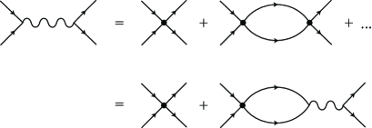
Figure 1: The diagrammatic representation of the fluctuation propagator. The solid lines are the Green’s functions of fermions in the normal state, the bold dots denote the BCS pairing potential.

The expression (II) is valid at all temperatures, for any pairing symmetry and band structure [we will keep only the linear in $\bm{q}$ term in the expansion (5), assuming that the band structure is such that the higher-order terms are negligible]. The solution $T(\bm{q},h)$ of the equation ${\cal L}^{-1}(\bm{q},0)=0$ determines the temperature at which the superconducting instability with the wave vector $\bm{q}$ develops in a given field $h$. Setting $\nu_{m}=\bm{q}=T=0$, one finds that the second-order quantum phase transition into a uniform superconducting state occurs at $h_{0}=(\pi/2e^{\mathbb{C}})T_{c0}=\Delta_{0}/2\simeq 0.88T_{c0}$, where $\Delta_{0}$ is the BCS gap at $T=0$. In general, the critical temperature vs field $T_{c}(h)$, or inversely the critical field vs temperature $h_{c}(T)$, can be found by maximizing $T(\bm{q},h)$ with respect to $\bm{q}$. According to Refs. LO64, ; FF64, , in a clean isotropic superconductor at $T<T^{*}\simeq 0.56T_{c0}$ the maximum of the critical field is achieved at $\bm{q}_{c}\neq 0$. The generic phase diagram of a LOFF superconductor is sketched in Fig. 2.

In the vicinity of the critical field $h_{c}(T)$, the most divergent contributions to physical quantities come from the low-frequency fluctuations, so the inverse fluctuation propagator (II) can be expanded in powers of $\nu_{m}$:

$$\frac{1}{N_{F}}{\cal L}^{-1}(\bm{q},\nu_{m})=A(\bm{q},h)+\tilde{A}(\bm{q},h)\frac{|\nu_{m}|}{2h}+O(\nu_{m}^{2}),$$ (6)

where

$$A(\bm{q},h) = \left\langle\phi_{\bm{k}}^{2}\,\mathrm{Re}\,\Psi\left(\frac{1}{2}+\frac{iW_{\bm{k}}}{4\pi T}\right)\right\rangle$$ (7)

$$-\Psi\left(\frac{1}{2}\right)+\ln\frac{T}{T_{c0}},$$

$$\tilde{A}(\bm{q},h) = \frac{h}{2\pi T}\left\langle\phi_{\bm{k}}^{2}\,\mathrm{Re}\,\Psi^{\prime}\left(\frac{1}{2}+\frac{iW_{\bm{k}}}{4\pi T}\right)\right\rangle.$$ (8)

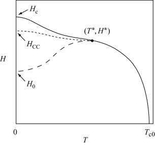
Figure 2: The generic phase diagram of the LOFF superconductor. The LOFF state appears at $H=H_{c}$ (solid line) at temperatures below the tricritical point $(T^{*},H^{*})$. The dashed lines correspond to the normal metal-to-uniform superconductor phase transitions: the first-order Clogston-Chandrasekhar transition at $H_{CC}$ (dashed line), and the second-order transition at $H_{0}$ (long-dashed line). The critical field of the LOFF state-to-uniform superconductor transition is not shown.

We focus on the fluctuation effects at $T=0$, when the explicit temperature dependence of the expressions (7) and (8) can be eliminated by using the asymptotic form of the digamma function: $\Psi(x)=\ln x+O(x^{-1})$ at $x\to\infty$ (Ref. AS65, ):

$$A(\bm{q},h) = \ln\frac{h}{h_{0}}+F(\bm{Q}),$$ (9)

$$\tilde{A}(\bm{q},h) = \tilde{F}(\bm{Q}),$$ (10)

where $\bm{Q}=\bm{q}/2h$, and

$$F(\bm{Q}) = \left\langle\phi_{\bm{k}}^{2}\ln|\bm{v}_{\bm{k}}\bm{Q}-1|\right\rangle,$$ (11)

$$\tilde{F}(\bm{Q}) = \pi\left\langle\phi_{\bm{k}}^{2}\delta(\bm{v}_{\bm{k}}\bm{Q}-1)\right\rangle$$ (12)

If the function $F(\bm{Q})$ has a minimum at $\bm{Q}=\bm{Q}_{c}$, then the upper critical field is given by $h_{c}=h_{0}e^{-F(\bm{Q}_{c})}$, and the equilibrium wave vector of the LOFF structure is $\bm{q}_{c}=2h_{c}\bm{Q}_{c}$.

In the standard theory of superconducting fluctuations, see Ref. LV-book, , it is assumed that the maximum of the critical temperature, or of the critical field, is achieved for the uniform superconducting state, which makes it possible to expand ${\cal L}^{-1}(\bm{q},\nu_{m})$ in the vicinity of the origin in the momentum space. In contrast, the most important critical fluctuations in the LOFF state have the wave vectors near $\bm{q}_{c}\neq 0$. Assuming that $F(\bm{Q})$ can be expanded in the Taylor series near the minimum, we obtain the following expression for the fluctuation propagator:

$${\cal L}(\bm{q},\nu_{m})$$

$$\quad=\frac{1}{N_{F}}\frac{1}{\epsilon+\gamma|\nu_{m}|+K_{ij}(q_{i}-q_{c,i})(q_{j}-q_{c,j})},\quad$$ (13)

where

$$\epsilon=\frac{h-h_{c}}{h_{c}}$$ (14)

measures the distance to the quantum critical point,

$$\gamma=\frac{\tilde{F}(\bm{Q}_{c})}{2h_{c}},$$ (15)

and $K_{ij}=(1/8h_{c}^{2})\nabla_{i}\nabla_{j}F(\bm{Q}_{c})$, $i,j=x,y,z$. In should be noted that in some cases the frequency expansion (6) of the inverse fluctuation propagator does not exist, see Sec. II.3 below.

II.1 Isotropic 3D case

Explicit expressions for $\gamma$ and $K_{ij}$ can only be obtained in few cases, including a 3D parabolic band, $\xi_{\bm{k}}=\bm{k}^{2}/2m-\mu$, with isotropic pairing. In this case a straightforward integration in Eqs. (11,12) gives

$$F(\bm{Q}) = \frac{1}{2}\ln|x^{2}-1|+\frac{1}{2x}\ln\left|\frac{x+1}{x-1}\right|-1,$$ (16)

$$\tilde{F}(\bm{Q}) = \frac{\pi}{2x}\theta(x-1)$$ (17)

where $x=v_{F}Q=v_{F}q/2h$. The function (16) has a minimum at $x=x_{c}\simeq 1.20$, with $F(\bm{Q}_{c})\simeq-0.41$, see Fig. 3. Thus the quantum phase transition occurs at $h_{c}\simeq 1.51h_{0}\simeq 0.75\Delta_{0}$, and at $h<h_{c}$ the superconducting order parameter is spatially modulated, with the wave vector $q_{c}=2x_{c}h_{c}/v_{F}\simeq 0.51\xi_{0}^{-1}$, where $\xi_{0}=v_{F}/2\pi T_{c0}$ is the BCS coherence length. The LOFF critical field $h_{c}$ exceeds not only $h_{0}$, but also the Clogston-Chandrasekhar field $h_{CC}=\Delta_{0}/\sqrt{2}$, which corresponds to a first-order phase transition between the normal and the uniform superconducting states,Clog62 ; Chan62 see Fig. 2.

Figure 3: The momentum dependence of ${\cal L}^{-1}(\bm{q},0)$ in the isotropic 3D case, Eq. (16) (solid line), and the isotropic 2D case, Eq. (22) (dashed line); $x=v_{F}|\bm{q}|/2h$.

In the isotropic case the critical field of the LOFF state does not depend on the direction of $\bm{q}$, and the quantum-critical fluctuation propagator (II) takes the following form:

$${\cal L}(\bm{q},\nu_{m})=\frac{1}{N_{F}}\frac{1}{\epsilon+\gamma|\nu_{m}|+K(|\bm{q}|-q_{c})^{2}},$$ (18)

where $\gamma\simeq 0.65/h_{c}$ and $K\simeq 0.28v_{F}^{2}/h_{c}^{2}$. The static limit of Eq. (18) has the same form as the propagator of classical fluctuations of the order parameter associated with the crystallization transition in an isotropic liquid.Braz75 Note also that the minimum of ${\cal L}^{-1}(\bm{q},0)$ remains infinitely degenerate even for an ellipsoidal Fermi surface, $\xi_{\bm{k}}=\sum_{i}k_{i}^{2}/2m_{i}-k_{F}^{2}/2m$, where $m_{i}=m/\mu_{i}^{2}$ are the effective masses, $i=x,y,z$. In this case, a change of variables reduces the fluctuation propagator to the form (18), in which $|\bm{q}|\to\sqrt{\mu_{x}^{2}q_{x}^{2}+\mu_{y}^{2}q_{y}^{2}+\mu_{z}^{2}q_{z}^{2}}$. Therefore, the critical field has the same value as in the isotropic case, the only difference being that the degeneracy manifold in the momentum space is now ellipsoidal rather than spherical.

II.2 Generic band structure

The infinite degeneracy of the LOFF states is an artifact of the parabolic band approximation. It will be lifted in the case of a general band structure or an anisotropic gap symmetry. Since $A(g^{-1}\bm{q},h)=A(\bm{q},h)$, where $g$ is an arbitrary element of the point group ${\cal G}$, the minima of the inverse fluctuation propagator in the momentum space form a “star”, i.e. a set of $N_{q}$ isolated points, $\{\bm{q}_{c}^{(a)}\}$, which is invariant under all operations from ${\cal G}$. Assuming that inversion is present in the point group, $N_{q}$ can be as low as two and as high as the total number of the group elements in ${\cal G}$. The equilibrium order parameter just below the critical field can be represented as a linear combination of the plane waves:

$$\eta(\bm{r})=\sum_{a=1}^{N_{q}}\eta_{a}e^{i\bm{q}_{c}^{(a)}\bm{r}}.$$ (19)

The complex coefficients $\eta_{a}$, which determine the spatial structure of the LOFF phase, are found by minimizing the Ginzburg-Landau free energy. If the minima of $A(\bm{q},h)$ are well-separated then the fluctuation modes near different $\bm{q}_{c}^{(a)}$ can be treated independently.

Let us consider for concreteness a tetragonal crystal with ${\cal G}=\mathbf{D}_{4h}$, in which case there can be as many as sixteen degenerate minima of $A(\bm{q},h)$. This number is severely reduced if one assumes that $\bm{q}_{c}^{(a)}$ are along the highest symmetry directions. For a 3D band this means that $N_{q}=2$, with $\bm{q}_{c}^{(1,2)}=\pm q_{c}\hat{z}$. Near the minima, one can write $A_{1,2}(\bm{q},h)=\epsilon+K_{\parallel}(q_{z}\mp q_{c})^{2}+K_{\perp}(q_{x}^{2}+q_{y}^{2})$. On the other hand, if there are 2D bands in the system, then the lowest possible number of the minima is four, located for instance at $\bm{q}_{c}^{(1,3)}=\pm q_{c}\hat{x}$, $\bm{q}_{c}^{(2,4)}=\pm q_{c}\hat{y}$. Then, $A_{1}(\bm{q},h)=\epsilon+K_{\parallel}(q_{x}-q_{c})^{2}+K_{\perp}q_{y}^{2}$, etc. Without any loss of generality, we can assume that $K_{\parallel}=K_{\perp}=K$, so that the fluctuation propagator near the $a$th minimum can be written in the following form:

$${\cal L}_{a}(\bm{q},\nu_{m})=\frac{1}{N_{F}}\frac{1}{\epsilon+\gamma|\nu_{m}|+K\left(\bm{q}-\bm{q}_{c}^{(a)}\right)^{2}}.$$ (20)

This expression, in which $\gamma$ and $K$ should be treated as phenomenological constants, is applicable in the generic case of a 3D or 2D crystalline superconductor with arbitrary band structure and pairing symmetry.

We would like to note the formal similarity between our superconducting fluctuation propagators (18) and (20) and the propagators of magnetic fluctuations in itinerant helical ferromagnetsST04 and high-$T_{c}$ superconductors,MMP90 respectively.

II.3 Isotropic 2D case

The fluctuation propagator does not have the simple form (II) if $\gamma$ is either zero or infinity. According to Eq. (12), the former possibility occurs if the surface $\bm{v}_{\bm{k}}\bm{Q}_{c}=1$ does not intersect the Fermi surface, or if it does then $\phi_{\bm{k}}$ accidentally vanishes on the intersection line. In either case one would have to go to higher orders of the frequency expansion. We have not been able to find an explicit example of the band structure for which this happens.

If $\gamma=\infty$ then the Taylor expansion in powers of $|\nu_{m}|$ fails, and one to take the low-temperature limit directly in Eq. (II). Assuming as before that the temperature is the smallest energy scale in the system, one obtains:

$$\frac{1}{N_{F}}{\cal L}^{-1}(\bm{q},\nu_{m})=\ln\frac{h}{h_{0}}$$

$$\quad+\,\mathrm{Re}\,\left\langle\phi_{\bm{k}}^{2}\ln\left(\frac{\bm{v}_{\bm{k}}\bm{q}}{2h}-1-i\frac{|\nu_{m}|}{2h}\right)\right\rangle.$$ (21)

In order to recover the expressions (9,10) from this, one has to replace $|\nu_{m}|\to|\nu_{m}|+0^{+}$.

One can check that the frequency expansion fails in the case of the isotropic 2D band with $\xi_{\bm{k}}=(k_{x}^{2}+k_{y}^{2})/2m-\mu$ and $\phi_{\bm{k}}=1$. For the order parameter modulated in the $xy$ plane we have

$$F(\bm{Q})=\,\mathrm{Re}\,\ln\frac{1+\sqrt{1-x^{2}}}{2},$$ (22)

$$\tilde{F}(\bm{Q})=\frac{1}{\sqrt{x^{2}-1}}\theta(x-1)$$ (23)

where $x=v_{F}Q=v_{F}q/2h$. The function $F(\bm{Q})$ has a non-analytical minimum at $x=1$, with $F(\bm{Q}_{c})=-\ln 2$, see Fig. 3. Therefore the zero-temperature critical field is $h_{c}=2h_{0}$, and the LOFF wave vector is $q_{c}=4h_{0}/v_{F}$. Since $\tilde{F}$ diverges at the critical point, one has to use Eq. (II.3), with the following result:

$$\frac{1}{N_{F}}{\cal L}^{-1}(\bm{q},\nu_{m})=\ln\frac{h}{h_{0}}+{\cal F}\left(\frac{v_{F}|\bm{q}|}{2h},\frac{|\nu_{m}|}{2h}\right),$$ (24)

where

$${\cal F}(x,y)=\,\mathrm{Re}\,\ln\frac{1+iy+\sqrt{(1+iy)^{2}-x^{2}}}{2}.$$

We see that the retarded fluctuation propagator ${\cal L}^{R}(\bm{q},\nu)$ obtained from Eq. (24) has a branch cut instead of a simple pole.

The non-analyticity of the inverse fluctuation propagator persists even if the Fermi surface is a corrugated cylinder. For the quasi-2D band described by $\xi_{\bm{k}}=(k_{x}^{2}+k_{y}^{2})/2m-t\cos k_{z}d-\mu$ ($t\ll\mu$), with isotropic pairing, one can show that the deepest minimum of $A(\bm{q},h)$ is achieved for $\bm{q}\parallel\hat{z}$.ADF74 Then, $F(\bm{Q})$ and $\tilde{F}(\bm{Q})$ are given by the same expressions (22) and (23) as in the 2D case, but with $x=td|q_{z}|/2h$. The divergence of $\tilde{F}$ at $x=1$ again signals the failure of the expansion of ${\cal L}^{-1}(\bm{q},\nu_{m})$ in powers of frequency.

Below we neglect these complications and assume that the fluctuation propagator has either the form (18) or (20). This does not seem to be very restrictive, especially since a well-defined frequency expansion and analytical momentum dependence will be restored in realistic layered superconductors by the Fermi-surface or gap anisotropy, or by disorder.

III Fluctuation corrections

III.1 Free energy and spin susceptibility

If the quantum LOFF transition in the isotropic 3D case is first order,BR02 ; MC04 then our theory is not applicable. However, even in that case it is still instructive to do the calculations using the fluctuation propagator (18) in order to highlight the differences with the generic case. The fluctuation correction to the free energy in the normal state at $T=0$ is given by

$$\delta F=2\sum_{\bm{q}}\int_{0}^{\nu_{\max}}\frac{d\nu}{2\pi}\ln{\cal L}^{-1}(\bm{q},\nu).$$ (25)

The momentum integration is restricted to $|\bm{q}|\leq q_{\max}$, see Sec. II. In addition, the ultraviolet cutoff $\nu_{\max}\simeq\omega_{\max}$ is introduced to guarantee the convergence of the frequency integral. This cutoff can be extended to infinity when calculating the correction to the magnetic susceptibility:

$$\delta\chi=-\frac{\partial^{2}}{\partial H^{2}}\delta F=-N_{F}^{2}\frac{1}{H_{c}^{2}}\frac{\partial^{2}}{\partial\epsilon^{2}}\delta F.$$

In the isotropic 3D case, using the fluctuation propagator (18), we have at $\epsilon\to 0$:

$$\delta\chi = \frac{N_{F}}{\pi\gamma H_{c}^{2}}\int\frac{d^{3}\bm{q}}{(2\pi)^{3}}\frac{1}{\epsilon+K(|\bm{q}|-q_{c})^{2}}$$ (26)

$$\simeq \frac{N_{F}q_{c}^{2}}{2\pi^{2}\gamma H_{c}^{2}\sqrt{K}}\frac{1}{\sqrt{\epsilon}}$$

(the main contribution to the integral comes from the vicinity of $q_{c}\ll q_{\max}$). To estimate the magnitude of the correction, we compare it to the Pauli spin susceptibility in the normal state, $\chi_{P}=2\mu_{B}^{2}N_{F}$:

$$\frac{\delta\chi}{\chi_{P}}\simeq 1.21\left(\frac{\Delta_{0}}{\epsilon_{F}}\right)^{2}\left(\frac{H_{c}}{H-H_{c}}\right)^{1/2},$$ (27)

where $\epsilon_{F}=k_{F}^{2}/2m$ is the Fermi energy. Although this expression is divergent at the quantum critical point, the size of the fluctuation correction at any nonzero $\epsilon$ is small because of the factor $\left(\Delta_{0}/\epsilon_{F}\right)^{2}$. The width of the fluctuation region in this case can be estimated as $(H-H_{c})/H_{c}\sim\left(\Delta_{0}/\epsilon_{F}\right)^{4}$. Note also that the field-dependent fluctuation contribution to the magnetization,

$$\delta M=-\frac{\partial}{\partial H}\delta F=-N_{F}\frac{1}{H_{c}}\frac{\partial}{\partial\epsilon}\delta F,$$

is of the type $\delta M\propto\sqrt{\epsilon}$, and is not singular at $\epsilon\rightarrow 0$.

In the generic 3D case, using Eq. (20) we obtain:

$$\delta\chi=\frac{N_{F}}{\pi\gamma H_{c}^{2}}\sum_{a}\int\frac{d^{3}\bm{q}}{(2\pi)^{3}}\frac{1}{\epsilon+K\left(\bm{q}-\bm{q}_{c}^{(a)}\right)^{2}}.$$ (28)

Then, for each minimum $\bm{q}_{c}^{(a)}$, the integral can be calculated by shifting the integration variable, $\bm{q}-\bm{q}_{c}^{(a)}=\bm{p}$:

$$\delta\chi = \frac{N_{F}}{\pi\gamma H_{c}^{2}}\sum_{a}\int\frac{d^{3}\bm{p}}{(2\pi)^{3}}\frac{1}{\epsilon+K\bm{p}^{2}}$$ (29)

$$= N_{q}\frac{N_{F}q_{\max}}{2\pi^{3}H_{c}^{2}\gamma K}\left(1-\frac{\pi}{2q_{\max}}\sqrt{\frac{\epsilon}{K}}\right),$$

which is not singular at $\epsilon\to 0$, so is the correction to the magnetization.

In contrast, in the generic 2D case with isolated minima the reduced dimensionality of the momentum integral leads to a logarithmic singularity in $\delta\chi$:

$$\delta\chi = \frac{N_{F}}{\pi\gamma H_{c}^{2}}\sum_{a}\int\frac{d^{2}\bm{p}}{(2\pi)^{2}}\frac{1}{\epsilon+K\bm{p}^{2}}$$ (30)

$$= N_{q}\frac{N_{F}}{4\pi^{2}H_{c}^{2}\gamma K}\ln\frac{Kq_{\max}^{2}}{\epsilon}.$$

Using $\gamma\sim 1/h_{c}$ and $K\sim v_{F}^{2}/h_{c}^{2}$, we have the following estimate for the quantum fluctuation correction to the susceptibility:

$$\frac{\delta\chi}{\chi_{P}}\sim\frac{\Delta_{0}}{\epsilon_{F}}\ln\frac{H_{c}}{H-H_{c}}.$$ (31)

Our analysis can be easily extended to the case of the normal metal-to-uniform superconductor transition (one should remember though that in a paramagnetically-limited clean superconductor this transition does not exist, since the LOFF instability always preempts the uniform instability at $T=0$). Formally setting $\bm{q}_{c}=0$ in the fluctuation propagator, we see that the infinitely degenerate case (26) is never realized and the correction to $\chi$ in three dimensions is non-singular, see Eq. (29). In the 2D case, one would have the logarithmically divergent correction (30).

III.2 Quasiparticle decay rate

The lowest-order contribution to the self-energy of spin-up fermions due to the superconducting fluctuations in the normal state is given by

$$\Sigma_{\uparrow}(\bm{k},\omega_{n}) = -T\sum_{m}\sum_{\bm{q}}{\cal L}(\bm{q},\nu_{m})$$ (32)

$$\times G_{\downarrow}\left(-\bm{k}+\bm{q},-\omega_{n}+\nu_{m}\right),$$

see Fig. 4, where $G_{\downarrow}(\bm{k},\omega_{n})=(i\omega_{n}-\xi_{\bm{k}}-h)^{-1}$ is the Green’s function of spin-down fermions (the pairing is assumed to be isotropic). At $T=0$ we obtain for the quasiparticle decay rate at the spin-up Fermi surface, i.e. for $\bm{k}$ satisfying $\xi_{\bm{k}}=h$:

$$\Gamma(\hat{\bm{k}},\omega)\equiv-\,\mathrm{Im}\,\Sigma^{R}_{\uparrow}(\hat{\bm{k}},\omega)=\sum_{\bm{q}}\,\mathrm{Im}\,{\cal L}^{R}(\bm{q},\omega-W_{\bm{k}}),$$ (33)

where $\hat{\bm{k}}$ is the direction of the Fermi momentum, ${\cal L}^{R}(\bm{q},\nu)$ is the retarded fluctuation propagator, and the integration is restricted to the region in the $\bm{q}$-space defined by the condition $0\leq W_{\bm{k}}\leq\omega$. Below we calculate the decay rate in the limit $\omega\to 0$ at the quantum critical point, i.e. at $\epsilon=0$.

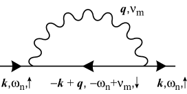
Figure 4: The contribution of superconducting fluctuations to the fermion self-energy, Eq. (32). The solid lines are the single-particle Green’s functions. The wavy line is the fluctuation propagator ${\cal L}(\bm{q},\nu_{m})$.

In the isotropic 3D case the fluctuation propagator is given by Eq. (18). It is convenient to choose the polar axis in the $\bm{q}$-space along $\bm{v}_{\bm{k}}=v_{F}\hat{\bm{k}}$ (we neglect the difference between the quasiparticle velocity at the spin-up Fermi surface and the Fermi velocity $v_{F}$, which is of the order of $h_{c}/\epsilon_{F}$). It is easy to see that the decay rate in this case does not depend on $\hat{\bm{k}}$:

$$\Gamma(\omega) = \frac{\gamma}{4\pi^{2}N_{F}}\int_{-1}^{1}ds$$

$$\times\int_{0}^{\infty}q^{2}dq\frac{\omega-W_{\bm{k}}}{K^{2}(q-q_{c})^{4}+\gamma^{2}(\omega-W_{\bm{k}})^{2}}$$

($s=\cos\theta$). Since the main contribution to the integral comes from from $q\simeq q_{c}$, one can replace $W_{\bm{k}}\to v_{F}q_{c}s-2h_{c}$. Introducing $u=\omega-W_{\bm{k}}$, we have

$$\Gamma(\omega) = \frac{\sqrt{2}}{8\pi}\frac{q_{c}}{N_{F}v_{F}\sqrt{\gamma K}}\int_{u_{\min}}^{u_{\max}}du\,u^{-1/2}$$ (34)

$$= \frac{\sqrt{2}}{4\pi}\frac{q_{c}}{N_{F}v_{F}\sqrt{\gamma K}}\omega^{1/2},$$

where $u_{\min}=\max\{0,\omega-v_{F}q_{c}+2h_{c}\}=0$, $u_{\max}=\min\{\omega,\omega+v_{F}q_{c}+2h_{c}\}=\omega$ (we assume $\omega\ll h_{c}$). This expression takes a more transparent form if compared to the energy scale associated with the superconducting phase transition:

$$\frac{\Gamma(\omega)}{\Delta_{0}}\simeq 1.57\left(\frac{\Delta_{0}}{\epsilon_{F}}\right)^{2}\left(\frac{\omega}{\Delta_{0}}\right)^{1/2}.$$ (35)

We see that at the quantum phase transition into the LOFF state the Fermi-liquid behavior is destroyed by the superconducting fluctuations, and the magnitude of the fluctuation contribution to the decay rate is determined by the factor $\left(\Delta_{0}/\epsilon_{F}\right)^{2}$.

In the generic case, when the inverse fluctuation propagator has minima at isolated points $\bm{q}_{c}^{(a)}$ in the momentum space, see Eq. (20), the quasiparticle decay rate can be written as the sum of the independent contributions from each minimum:

$$\Gamma(\hat{\bm{k}},\omega)=\sum_{a}\Gamma_{a}(\hat{\bm{k}},\omega),$$ (36)

where

$$\Gamma_{a}=\frac{\gamma}{N_{F}}\int\frac{d^{D}\bm{q}}{(2\pi)^{D}}\frac{\omega-W_{\bm{k}}}{K^{2}\left(\bm{q}-\bm{q}_{c}^{(a)}\right)^{4}+\gamma^{2}(\omega-W_{\bm{k}})^{2}}.$$

Here the integration is restricted by the condition $0\leq W_{\bm{k}}\leq\omega$, and $D=3$ or $2$ is the dimensionality of the system.

In three dimensions, after changing the variables $\bm{q}-\bm{q}_{c}^{(a)}=\bm{p}$, choosing the $z$ axis in the momentum space along $\bm{v}_{\bm{k}}$, and introducing $u=\omega-w_{a}-|\bm{v}_{\bm{k}}|p_{z}$, where $w_{a}=\bm{v}_{\bm{k}}\bm{q}_{c}^{(a)}-2h_{c}$, one obtains:

$$\Gamma_{a} = \frac{\gamma}{4\pi^{2}N_{F}|\bm{v}_{\bm{k}}|}\int_{0}^{\infty}dp_{\perp}p_{\perp}$$

$$\times\int_{0}^{\omega}\frac{du\;u}{K^{2}[p_{\perp}^{2}+(u-\omega+w_{a})^{2}/\bm{v}_{\bm{k}}^{2}]^{2}+\gamma^{2}u^{2}}.$$

In the limit $\omega\to 0$, one can neglect $u-\omega$ in the first term in the denominator and calculate the integral over $u$:

$$\Gamma_{a} = \frac{1}{8\pi^{2}N_{F}\gamma|\bm{v}_{\bm{k}}|}\int_{0}^{\infty}dp_{\perp}p_{\perp}$$ (37)

$$\times\ln\left[1+\frac{\gamma^{2}\omega^{2}}{K^{2}(p_{\perp}^{2}+w_{a}^{2}/\bm{v}_{\bm{k}}^{2})^{2}}\right].\quad$$

The result of the integration here essentially depends on whether $w_{a}$ is zero or not.

If $\hat{\bm{k}}$ is such that $w_{a}\neq 0$, then one can expand the logarithm in Eq. (37) at $\omega\to 0$ and calculate the momentum integral. Substituting the result in Eq. (36) we obtain

$$\Gamma(\hat{\bm{k}},\omega)=\frac{1}{16\pi^{2}}\frac{\gamma|\bm{v}_{\bm{k}}|}{N_{F}K^{2}\tilde{w}^{2}}\omega^{2},$$ (38)

where $\tilde{w}^{-2}=\sum_{a}w_{a}^{-2}$. The fluctuation contribution to the quasiparticle decay rate has the energy dependence characteristic of the Fermi liquid, and its magnitude can be estimated as follows:

$$\frac{\Gamma(\hat{\bm{k}},\omega)}{\Delta_{0}}\sim\left(\frac{\Delta_{0}}{\epsilon_{F}}\right)^{2}\left(\frac{\omega}{\Delta_{0}}\right)^{2}.$$ (39)

On the other hand, if, for some $\hat{\bm{k}}$, one of $w_{a}$’s is zero, then $\tilde{w}^{-2}$ diverges, making the expression (38) inapplicable. Setting $w_{a}=0$ in Eq. (37), one obtains that the decay rate at $\omega\to 0$ is dominated by the contribution from the $a$th minimum:

$$\Gamma(\hat{\bm{k}},\omega)=\frac{1}{16\pi}\frac{1}{N_{F}|\bm{v}_{\bm{k}}|K}\omega,$$ (40)

so that

$$\frac{\Gamma(\hat{\bm{k}},\omega)}{\Delta_{0}}\sim\left(\frac{\Delta_{0}}{\epsilon_{F}}\right)^{2}\frac{\omega}{\Delta_{0}}.$$ (41)

Thus, the following picture emerges: In the generic case, the energy dependence of the quasiparticle decay rate due to the interaction with superconducting fluctuations turns out to be strongly anisotropic on the Fermi surface. While $\Gamma\propto\omega^{2}$ is almost everywhere, one has a non-Fermi-liquid behavior, $\Gamma\propto\omega$, on the lines defined by the intersection of the surfaces $\bm{v}_{\bm{k}}\bm{q}_{c}^{(a)}=2h_{c}$ with the Fermi surface. For the consistency of our calculation we have to assume that these intersection lines do exist, otherwise the coefficient $\gamma$ would be zero, see the discussion at the beginning of Sec. II.3.

Similar conclusions can be obtained in the generic 2D case, in which the decay rate has the same form (36), where, instead of Eq. (37), we now have

$$\Gamma_{a} = \frac{1}{8\pi^{2}N_{F}\gamma|\bm{v}_{\bm{k}}|}\int_{-\infty}^{\infty}dp_{\perp}$$ (42)

$$\times\ln\left[1+\frac{\gamma^{2}\omega^{2}}{K^{2}(p_{\perp}^{2}+w_{a}^{2}/\bm{v}_{\bm{k}}^{2})^{2}}\right].\quad$$

If $w_{a}\neq 0$, then

$$\Gamma(\hat{\bm{k}},\omega)=\frac{1}{16\pi}\frac{\gamma\bm{v}_{\bm{k}}^{2}}{N_{F}K^{2}\tilde{w}^{3}}\omega^{2},$$ (43)

where $\tilde{w}^{-3}=\sum_{a}|w_{a}|^{-3}$. Using $\gamma\sim 1/h_{c}$ and $K\sim v_{F}^{2}/h_{c}^{2}$, we obtain

$$\frac{\Gamma(\hat{\bm{k}},\omega)}{\Delta_{0}}\sim\frac{\Delta_{0}}{\epsilon_{F}}\left(\frac{\omega}{\Delta_{0}}\right)^{2}.$$ (44)

At the points on the Fermi surface where $w_{a}=0$, we have the expression

$$\Gamma(\hat{\bm{k}},\omega)=\frac{\sqrt{2}}{4\pi}\frac{1}{N_{F}|\bm{v}_{\bm{k}}|\sqrt{\gamma K}}\omega^{1/2},$$ (45)

whose magnitude can be estimated as

$$\frac{\Gamma(\hat{\bm{k}},\omega)}{\Delta_{0}}\sim\frac{\Delta_{0}}{\epsilon_{F}}\left(\frac{\omega}{\Delta_{0}}\right)^{1/2}.$$ (46)

Similar to the generic 3D case, the fluctuation contribution to the decay rate strongly depends on the direction of the Fermi momentum, showing non-Fermi-liquid behavior along some directions. Although the overall magnitude of the correction is larger than in the generic 3D case, it is still proportional to the small parameter $\Delta_{0}/\epsilon_{F}$. It is interesting to note that the same frequency dependence of the decay rate can be obtained in the model of a nearly antiferromagnetic Fermi liquid in 2D, where the quasiparticle interaction with spin fluctuations becomes anomalously strong near some points, the “hot spots”, on the Fermi line.HR95

Let us now compare our results with the decay rate at the second-order phase transition into the uniform superconducting state. Setting $\bm{q}_{c}=0$ and assuming an isotropic band dispersion, we have

$$\Gamma(\omega)=\frac{\gamma}{N_{F}}\int\frac{d^{D}\bm{q}}{(2\pi)^{D}}\frac{\omega-W_{\bm{k}}}{K^{2}\bm{q}^{4}+\gamma^{2}(\omega-W_{\bm{k}})^{2}},$$ (47)

instead of Eq. (36). In the 3D case, repeating the calculation steps leading to Eq. (38), one obtains:

$$\Gamma(\omega)=\frac{1}{64\pi^{2}}\frac{\gamma v_{F}}{N_{F}K^{2}\tilde{h}_{c}^{2}}\omega^{2}.$$ (48)

Similarly, in the 2D case,

$$\Gamma(\omega)=\frac{1}{128\pi}\frac{\gamma v_{F}^{2}}{N_{F}K^{2}h_{c}^{3}}\omega^{2}.$$ (49)

Thus, the Fermi-liquid character of quasiparticle excitations is not destroyed by the quantum fluctuations at the normal metal-to-uniform superconductor transition.

IV Conclusions and outlook

We have studied the order parameter fluctuations near the quantum phase transition at $H=H_{c}$ from the normal state to the LOFF superconducting state. We derived the general form of the fluctuation propagator ${\cal L}(\bm{q},\nu_{m})$ at finite $\bm{q}$ and $\nu_{m}$. In the systems suggested as good candidates for the experimental realization of the LOFF state, disorder is small or absent altogether. In the absence of impurity effects, we analyzed the momentum and frequency dependence of the fluctuation propagator in both isotropic 3D and 2D cases, as well as in the case of generic spectrum.

The fluctuation effects are more pronounced in the isotropic 3D case compared to the generic situation. This is because in the isotropic case the LOFF states are infinitely degenerate leading to the large phase volume of fluctuations. The fluctuation contribution to the spin susceptibility diverges at $H\to H_{c}$, $\delta\chi\propto(H-H_{c})^{-1/2}$, and the quasiparticle decay rate shows a non-Fermi-liquid behavior, $\Gamma(\omega)\propto\omega^{1/2}$, at the quantum critical point. The magnitude of the fluctuation corrections is determined by the parameter $(\Delta_{0}/\epsilon_{F})^{2}$. Although this ratio is very small in conventional bulk superconductors, it can vary in a wide range in the atomic Fermi gases. It should be noted that our results rely on the assumption that the LOFF transition at $T=0$ is of second order. As mentioned in the Introduction, this might not be the case in clean isotropic systems in the weak-coupling limit. However, as the ratio $\Delta_{0}/\epsilon_{F}$ grows so do the strong-coupling corrections to the mean-field free energy, which could stabilize the second-order LOFF transition. More theoretical work is needed to check if this possibility can indeed be realized.

In the generic case, which is expected to be applicable to crystalline paramagnetically-limited superconductors, or to the atomic Fermi gases in optical lattices, the equilibrium wave vectors of the LOFF state form a set of isolated points in the momentum space. The phase volume of fluctuations is reduced, resulting in a non-singular spin susceptibility in the 3D case, and a weak, logarithmic, divergence of $\delta\chi$ in the 2D case. Interestingly, the fluctuations in the generic case are still strong enough to cause the breakdown of the Fermi liquid at the quantum critical point, which manifests itself in a highly anisotropic energy dependence of the quasiparticle decay rate on the Fermi surface: $\Gamma(\omega)\propto\omega$ on some lines in 3D, and $\Gamma(\omega)\propto\omega^{1/2}$ at some points in 2D. We expect that the Fermi-liquid behavior, $\Gamma(\omega)\propto\omega^{2}$, will be restored throughout the Fermi surface away from the quantum critical point or in the presence of disorder, leaving the details for a future publication.

There is a number of open questions concerning the assumptions we made and the effects we neglected in the present study, the order of the quantum phase transition into the LOFF state being particularly important. Even if the mean-field transition is of second order, this might no longer be the case if one takes into account the fluctuation renormalization of the free energy. Additional complications arise in realistic crystalline superconductors, in which the orbital effects and disorder should be included. Finally, it would be interesting to extend our calculation of the fluctuation corrections to nonzero temperatures in the critical region around the LOFF transition.

References

- (1) M. Tinkham, Introduction to Superconductivity (McGraw-Hill, New York, 1996).
- (2) A. I. Larkin and Yu. N. Ovchinnikov, Zh. Eksp. Teor. Fiz. 47, 1136 (1964) [Sov. Phys. – JETP 20, 762 (1965)].
- (3) P. Fulde and R. A. Ferrell, Phys. Rev. 135, A550 (1964).
- (4) A. M. Clogston, Phys. Rev. Lett. 9, 266 (1962).
- (5) B. S. Chandrasekhar, Appl. Phys. Lett. 1, 7 (1962).
- (6) K. Maki, Physics 1, 127 (1964).
- (7) L. W. Gruenberg and L. Gunther, Phys. Rev. Lett. 16, 996 (1966).
- (8) A. A. Abrikosov, Zh. Eksp. Teor. Fiz. 32, 1442 (1957) [Sov. Phys. – JETP 5, 1174 (1957)].
- (9) E. Helfand and N. R. Werthamer, Phys. Rev. Lett. 13, 686 (1964).
- (10) L. N. Bulaevskii, Zh. Eksp. Teor. Fiz. 65, 1278 (1973) [Sov. Phys. – JETP 38, 634 (1974)].
- (11) H. Shimahara and D. Rainer, J. Phys. Soc. Jpn. 66, 3591 (1997).
- (12) K. Aoi, W. Dieterich, and P. Fulde, Z. Phys. 267, 223 (1974).
- (13) P. Fulde, Adv. Phys. 22, 667 (1973).
- (14) V. Barzykin and L. P. Gor’kov, Phys. Rev. Lett. 89, 227002 (2002).
- (15) L. G. Aslamazov, Zh. Eksp. Teor. Fiz. 55, 1477 (1968) [Sov. Phys. – JETP 28, 773 (1969)].
- (16) L. N. Bulaevskii and A. A. Guseinov, Fiz. Niz. Temp. 2, 283 (1976) [Sov. J. Low Temp. Phys. 2, 140 (1976)].
- (17) K. Gloos, R. Modler, H. Schimanski, C. D. Bredl, C. Geibel, F. Steglich, A. I. Buzdin, N. Sato, and T. Komatsubara, Phys. Rev. Lett. 70, 501 (1993).
- (18) R. Modler, P. Gegenwart, M. Lang, M. Deppe, M. Weiden, T. Lühmann, C. Geibel, F. Steglich, C. Paulsen, J. L. Tholence, N. Sato, T. Komatsubara, Y. Onuki, M. Tachiki, and S. Takahashi, Phys. Rev. Lett. 76, 1292 (1996).
- (19) F. Thomas, B. Wand, T. Lühmann, P. Gegenwart, G. R. Stewat, F. Steglich, J. P. Brison, A. Buzdin, L. Glemot, and J. Floquet, J. Low Temp. Phys. 102, 117 (1995).
- (20) H. Burkhardt and D. Rainer, Ann. Phys. 3, 181 (1994).
- (21) N. Dupuis, Phys. Rev. B 51, 9074 (1995).
- (22) H. Shimahara, J. Phys. Soc. Jpn. 66, 541 (1997).
- (23) M. Houzet, A. Buzdin, L. Bulaevskii, and M. Maley, Phys. Rev. Lett. 88, 227001 (2002).
- (24) J. Singleton, J. A. Symington, M.-S. Nam, A. Ardavan, M. Kurmoo, and P. Day, J. Phys.: Condens. Matter 12, L641 (2000).
- (25) S. Manalo and U. Klein, J. Phys.: Condens. Matter 12, L471 (2000).
- (26) M. A. Tanatar, T. Ishiguro, H. Tanaka, and H. Kobayashi, Phys. Rev. B 66, 134503 (2002).
- (27) J. L. O’Brien, H. Nakagawa, A. S. Dzurak, R. G. Clark, B. E. Kane, N. E. Lumpkin, R. P. Starrett, N. Muira, E. E. Mitchell, J. D. Goettee, D. G. Rickel, and J. S. Brooks, Phys. Rev. B 61, 1584 (2000).
- (28) H. A. Radovan, N. A. Fortune, T. P. Murphy, S. T. Hannahs, E. C. Palm, S. W. Tozer, D. Hall, Nature 425, 51 (2003).
- (29) A. Bianchi, R. Movshovich, C. Capan, P. G. Pagliuso, and J. L. Sarrao, Phys. Rev. Lett. 91, 187004 (2003).
- (30) W. E. Pickett, R. Weht, and A. B. Shick, Phys. Rev. Lett. 83, 3713 (1999).
- (31) M. W. Zwierlein, A. Schirotzek, C. H. Schunck, and W. Ketterle, preprint cond-mat/0511197.
- (32) G. B. Partridge, W. Li, R. I. Kamar, Y. Liao, and R. G. Hulet, preprint cond-mat/0511752.
- (33) R. Combescot, Europhys. Lett. 55, 150 (2001).
- (34) T. Mizushima, K. Machida, and M. Ichioka, Phys. Rev. Lett. 94, 060404 (2005).
- (35) A. Sedrakian, J. Mur-Petit, A. Polls, and H. Müther, Phys. Rev. A 72, 013613 (2005).
- (36) D. E. Sheehy and L. Radzihovsky, preprint cond-mat/0508430.
- (37) J. Dukelsky, G. Ortiz, and S. M. A. Rombouts, preprint cond-mat/0510635.
- (38) A. I. Buzdin and H. Kachkachi, Phys. Letters A 225, 341 (1997).
- (39) D. F. Agterberg and K. Yang, J. Phys.: Condens. Matter 13, 9259 (2001).
- (40) U. Klein, D. Rainer, and H. Shimahara, J. Low. Temp. Phys. 118, 91 (2000).
- (41) M. Houzet and A. Buzdin, Phys. Rev. B 63, 184521 (2001).
- (42) H. Adachi and R. Ikeda, Phys. Rev. B 68, 184510 (2003).
- (43) K. Yang and A. H. MacDonald, Phys. Rev. B 70, 094512 (2004).
- (44) K. V. Samokhin, Physica C274, 156 (1997).
- (45) K. Yang and S. L. Sondhi, Phys. Rev. B 57, 8566 (1998).
- (46) A. B. Vorontsov, J. A. Sauls, and M. J. Graf, preprint cond-mat/0506257.
- (47) A. Malaspinas and T. M. Rice, Phys. Kondens. Materie 13, 193 (1971).
- (48) S. Matsuo, S. Higashitani, Y. Nagato, and K. Nagai, J. Phys. Soc. Jpn. 67, 280 (1998).
- (49) R. Casalbuoni and G. Tonini, Phys. Rev. B 69, 104505 (2004).
- (50) J. A. Bowers and K. Rajagopal, Phys. Rev. D 66, 065002 (2002).
- (51) C. Mora and R. Combescot, Phys. Rev. B 71, 214504 (2005).
- (52) H. Shimahara, J. Phys. Soc. Jpn. 67, 1872 (1998).
- (53) Y. Ohashi, J. Phys. Soc. Jpn. 71, 2625 (2002).
- (54) L. D. Landau and E. M. Lifshitz, Statistical Physics, Part 1, 3rd ed. (Butterworth-Heinemann, 1980).
- (55) S. A. Brazovskii, Zh. Eksp. Teor. Fiz. 68, 175 (1975) [Sov. Phys. – JETP 41, 85 (1975)].
- (56) D. Dalidovich and K. Yang, Phys. Rev. Lett. 93, 247002 (2004).
- (57) A. I. Larkin and A. A. Varlamov, Theory of Fluctuations in Superconductors (Oxford University Press, 2005).
- (58) R. Ramazashvili and P. Coleman, Phys. Rev. Lett. 79, 3752 (1997).
- (59) V. P. Mineev and M. Sigrist, Phys. Rev. B 63, 172504 (2001).
- (60) V. M. Galitski and A. I. Larkin, Phys. Rev. B 63, 174506 (2001).
- (61) V. M. Galitski and S. Das Sarma, Phys. Rev. B 67, 144501 (2003).
- (62) A. V. Lopatin, N. Shah, and V. M. Vinokur, Phys. Rev. Lett. 94, 037003 (2005).
- (63) V. P. Mineev and K. V. Samokhin, Introduction to Unconventional Superconductivity (Gordon and Breach, London, 1999).
- (64) M. Abramowitz and I. A. Stegun, Handbook of Mathematical Functions (Dover Publications, 1965).
- (65) J. Schmalian and M. Turlakov, Phys. Rev. Lett. 93, 036405 (2004).
- (66) A. J. Millis, H. Monien, and D. Pines, Phys. Rev. B 42, 167 (1990).
- (67) R. Hlubina and T. M. Rice, Phys. Rev. B 51, 9253 (1995).