A semiclassical theory of the Ehrenfest-time dependence of quantum transport in ballistic quantum dots

Abstract

We present a trajectory-based semiclassical calculation of the Ehrenfest-time dependence of the weak localization correction and the universal conductance fluctuations of a ballistic quantum dot with ideal point contacts. While the weak localization correction is proportional to $\exp(-\tau_{\rm E}/\tau_{\rm D})$, where $\tau_{\rm E}$ and $\tau_{\rm D}$ are the dot’s Ehrenfest time and dwell time, respectively, the variance of the conductance is found to be independent of $\tau_{\rm E}$. The latter is in agreement with numerical simulations of the quantum kicked rotator [Tworzydlo et al., Phys. Rev. B 69, 165318 (2004) and Jacquod and Sukhorukov, Phys. Rev. Lett. 92, 116801 (2004)].

I Introduction

Weak localization and universal conductance fluctuations are manifestations of quantum interference on quantum transport.Beenakker and van Houten (1991) How these effects appear in a ballistic quantum dot, coupled to source and drain reservoirs via ideal point contacts, is believed to depend on the ratio of the Ehrenfest time and the mean dwell time $\tau_{\rm D}$.Aleiner and Larkin (1996) The Ehrenfest time $\tau_{\rm E}$ is the time it takes for two classical trajectories, initially a Fermi wavelength apart, to diverge and be separated by a distance comparable to the system size.Larkin and Ovchinnikov (1968); Zaslavsky (1981) Trajectories need to remain inside the dot during at least a time $\tau_{\rm E}$ in order to contribute to weak localization or universal conductance fluctuations.

For the weak localization correction $\delta G$, semiclassical theory predicts that $\delta G\propto\exp(-\tau_{\rm E}/\tau_{\rm D})$,Aleiner and Larkin (1996); Adagideli (2003); Rahav and Brouwer (2005a); Brouwer and Rahav (2005); Jacquod and Whitney (2005) which has been verified using accurate numerical simulations of the quantum kicked rotatorRahav and Brouwer (2005a); Jacquod and Whitney (2005) — a “quantum dot” with “stroboscopic” dynamics.Tworzydlo et al. (2004a) For universal conductance fluctuations, numerical simulations found no Ehrenfest-time dependence of $\mbox{var}\,G$.Tworzydlo et al. (2004b); Jacquod and Sukhorukov (2004) This remarkable result remained unexplained because of the absence of a semiclassical theory of universal conductance fluctuations in ballistic quantum dots. It is the goal of this article to report such a theory and offer a microscopic explanation for the absence of Ehrenfest-time dependence of conductance fluctuations seen in the numerical simulations.

Two theoretical approaches have been taken to address quantum transport in ballistic quantum dots. One is the theory of Aleiner and Larkin,Aleiner and Larkin (1996) which considers quantum corrections to the ballistic analogue of the “diffuson” and “cooperon” propagators that play a central role in the diagrammatic perturbation theory for disordered conductors. The other approach is based on an expression relating the dot’s scattering matrix to a sum over classical trajectories connecting the two point contacts.Baranger et al. (1993a) In all cases where both approaches have been used to calculate the same observable, the results have been the same. In this article, we we use the trajectory-based approach.

In the trajectory-based semiclassical approach, the dot’s conductance $G$ is calculated from the Landauer formula,

$$G=\frac{2e^{2}}{h}T,$$ (1)

where $T$ is the total transmission of the dot. The transmission $T$ is expressed as a double sum over classical trajectories $\alpha$, $\beta$ that connect the two point contacts,Jalabert et al. (1990)

$$T=\frac{1}{(N_{1}+N_{2})\tau_{\rm D}}\sum_{\alpha,\beta}A_{\alpha}A_{\beta}e^{i(S_{\alpha}-S_{\beta})/\hbar}.$$ (2)

Here $A_{\alpha}$ and $A_{\beta}$ are stability amplitudes and $S_{\alpha}$ and $S_{\beta}$ are the classical actions of the two trajectories $\alpha$ and $\beta$. The classical trajectories $\alpha$ and $\beta$ start with initial transverse momentum compatible with the same mode $n$ in the left contact and end with transverse momentum compatible with the same mode $m$ in the right contact. The modes in each contact have quantized transverse momentum

$$p_{\perp}(m)=\pm\pi\hbar m/W_{j},\ \ m=1,\ldots,N_{j},$$ (3)

where $W_{j}$ is the width of the contact, $N_{j}$ the number of modes in the contact, and the subscript $j=1,2$ refers to the left and right contacts, respectively.

Weak localization is the small negative correction $\delta G$ to the ensemble average of the dot’s conductance $G$ arising from quantum interference. (The ensemble average is taken with respect to small variations of the shape of the quantum dot or the Fermi energy.) Two different trajectories $\alpha$ and $\beta$ contribute to weak localization if their action difference $S_{\alpha}-S_{\beta}$ is of order $\hbar$. Pairs of trajectories $\alpha$ and $\beta$ that contribute to weak localization are shown schematically in the top panel of Fig. 1. The two trajectories are almost equal, except for a stretch where $\beta$ has a small-angle self-intersection and $\alpha$ has a small-angle avoided self-intersection. Such pairs of trajectories were originally pointed out by Aleiner and Larkin;Aleiner and Larkin (1996) they were first investigated in the trajectory-based formalism by Sieber and Richter.Sieber and Richter (2001) The action difference between the two trajectories is of order $\hbar$ if the duration of the self-encounter is of order of the Ehrenfest time. The probability that the trajectories do not escape through the point contacts during the duration of the encounter is $\exp(-\tau_{\rm E}/\tau_{\rm D})$, hence the suppression $\delta G\propto\exp(-\tau_{\rm E}/\tau_{\rm D})$ of the weak localization correction for large Ehrenfest times mentioned previously.Aleiner and Larkin (1996); Adagideli (2003); Rahav and Brouwer (2005a); Jacquod and Whitney (2005); Brouwer and Rahav (2005)

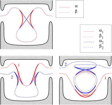
Figure 1: Top: schematic picture of a pair of interfering trajectories $\alpha$ and $\beta$ that give rise to the weak localization correction to the conductance. Bottom left and bottom right: schematic picture of quadruples of interfering trajectories $\alpha_{1}$, $\beta_{1}$, $\alpha_{2}$, and $\beta_{2}$ that contribute to conductance fluctuations. The true trajectories inside the dot are piecewise straight, with specular reflections off the dot’s boundary. The small-angle (self) encounters are shown thick. In the bottom right panel, the trajectories $\beta_{1}$ and $\alpha_{2}$ have one more revolution around a periodic trajectory (shown dotted) than their partners $\alpha_{1}$ and $\beta_{2}$.

Since the transmission $T$ is a double sum over classical trajectories $\alpha$ and $\beta$, the variance of the conductance is expressed as a quadruple sum over classical trajectories $\alpha_{1}$, $\beta_{1}$, $\alpha_{2}$, and $\beta_{2}$. Quadruples of trajectories for which the individual action differences $S_{\alpha_{1}}-S_{\beta_{1}}$ and $S_{\alpha_{2}}-S_{\beta_{2}}$ are large (so that they do not contribute to the average conductance), but the total action difference $S_{\alpha_{1}}+S_{\alpha_{2}}-S_{\beta_{1}}-S_{\beta_{2}}$ is small (of order $\hbar$) contribute to the conductance fluctuations. The two distinct classes of quadruples of trajectories that contribute to $\mbox{var}\,G$ are shown in the bottom panels of Fig. 1. Both classes have their counterpart in the theory of conductance fluctuations in diffusive conductors.Lee and Stone (1985); Altshuler and Shklovskii (1986)

The trajectories in the bottom left panel of Fig. 1 are the ones commonly associated with conductance fluctuations in ballistic quantum dotsJalabert et al. (1990); Baranger et al. (1993b); Takane and Nakamura (1998); Nakamura and Harayama (2004) (see, however, Ref. Argaman, 1996 for an exception). They undergo two small-angle encounters. The trajectories $\alpha_{1}$ and $\beta_{1}$, and $\alpha_{2}$ and $\beta_{2}$ are pairwise equal before the first encounter and after the last encounter. Between the encounters $\alpha_{1}$ and $\beta_{2}$, and $\alpha_{2}$ and $\beta_{1}$ are pairwise equal. The total action difference $S_{\alpha_{1}}+S_{\alpha_{2}}-S_{\beta_{1}}-S_{\beta_{2}}$ is of order $\hbar$ if the duration of each encounter $\gtrsim\tau_{\rm E}$. Since the survival probability during each encounter is $\exp(-\tau_{\rm E}/\tau_{\rm D})$, the contribution of these trajectories to $\mbox{var}\,G$ decreases $\propto\exp(-2\tau_{\rm E}/\tau_{\rm D})$ for large $\tau_{\rm E}$.

There is no exponential suppression at large Ehrenfest times for the trajectories shown in the bottom right panel of Fig. 1. Here, the trajectories $\beta_{1}$ and $\alpha_{2}$ differ from $\alpha_{1}$ and $\beta_{2}$, respectively, by one extra revolution around the same periodic trajectory (dotted). The additional revolution around a periodic trajectory ensures that the individual action differences $S_{\alpha_{1}}-S_{\beta_{2}}$ and $S_{\alpha_{2}}-S_{\beta_{2}}$ are large, whereas the total action difference $S_{\alpha_{1}}+S_{\alpha_{2}}-S_{\beta_{1}}-S_{\beta_{2}}$ is small if the trajectories $\alpha_{1}$ and $\beta_{2}$ spend at least a time $\tau_{\rm E}$ near the periodic trajectory. For a dot with mean dwell time $\tau_{\rm D}$, the typical period of a periodic trajectory (weighed with the square of the stability amplitudes) is of order $\tau_{\rm D}$. This means that the trajectories $\alpha_{1}$, $\beta_{1}$, $\alpha_{2}$, and $\beta_{2}$ need to wind many times around the periodic trajectory if they are to contribute to conductance fluctuations if $\tau_{\rm E}\gg\tau_{\rm D}$. However, since the survival probability of the trajectories $\sim\exp(-\tau_{\rm p}/\tau_{\rm D})$ depends on the period $\tau_{\rm p}$ of the periodic trajectory only, and not on the actual time $\sim\tau_{\rm E}$ spent inside the quantum dot, the contribution to the conductance fluctuations is not suppressed exponentially if $\tau_{\rm E}\gg\tau_{\rm D}$.

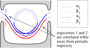
Figure 2: If the phase space distance between the trajectories $1$ and $2$ is of order $\hbar$ at the point when they arrive at or depart from the periodic trajectory, their motion is correlated for a time $\sim\tau_{\rm E}$ while away from the periodic trajectory. The contribution of such trajectories to the conductance fluctuations is suppressed if $\tau_{\rm E}\gg\tau_{\rm D}$. After the removal of trajectories with correlated motion away from the periodic trajectory the net contribution of the trajectories shown in the bottom right panel of Fig. 1 to the conductance fluctuations zero is finite.

This is not the full story, however. Periodic trajectories are related to density of states fluctuations via Gutzwiller’s trace formula,Gutzwiller (1990) so that trajectories of the type shown in the bottom right panel of Fig. 1 represent the impact of density-of-states fluctuations on the conductance. However, for chaotic quantum dots with ideal point contacts, the density of states and the conductance are known to be statistically independent,Brouwer et al. (1997) at least in the regime $\tau_{\rm E}\ll\tau_{\rm D}$ in which random matrix theory is valid. In other words, there is no Einstein relation for the conductance of a chaotic quantum dot with ideal point contacts if $\tau_{\rm E}\ll\tau_{\rm D}$. The same conclusion can be drawn based on the trajectory-based approach: Indeed, if one sums the contribution of trajectories of the type shown in the bottom right panel of Fig. 1 over all initial and final positions where the trajectories merge with or depart from the periodic trajectory, the net contribution to $\mbox{var}\,G$ vanishes.

The key observation that explains the existence of Ehrenfest-time independent conductance fluctuations in ballistic quantum dots is that the cancellation that is responsible for the vanishing of the density-of-states contribution to the conductance fluctuations is lifted if the dot’s Ehrenfest time $\tau_{\rm E}$ is large in comparison to the mean dwell time $\tau_{\rm D}$. This is because correlations between the trajectories shown in the bottom right panel of Fig. 1 persist away from the periodic trajectory if they approach the periodic trajectory and/or leave it at very close phase space points, as shown in Fig. 2. These additional correlations, which last up to a time $\tau_{\rm E}$, suppress the contribution of these trajectories to the conductance fluctuations if $\tau_{\rm E}\gg\tau_{\rm D}$, even if the two trajectories enter or exit through the same contact. After removing the trajectories with these additional correlations from the summation over all trajectories of the type shown in the bottom right panel of Fig. 1, the summation over the remaining trajectories no longer vanishes. The persistence of conductance fluctuations if $\tau_{\rm E}\gg\tau_{\rm D}$ thus can be attributed to all trajectories of the type shown in the bottom right panel of Fig. 1 that do not arrive at or depart from the periodic trajectory at close phase space points.

These qualitative arguments will be supported by the semiclassical calculations presented in the next three sections. We use the trajectory-based semiclassical formalism in the formulation developed in a series of works by Haake and collaborators.Müller et al. (2004, 2005); Heusler et al. (2006); Braun et al. (2005) In Ref. Heusler et al., 2006, Heusler et al. show how this formalism is applied to the calculation of the weak localization correction, correcting two canceling mistakes in the earlier theories of Refs. Richter and Sieber, 2002; Adagideli, 2003 (see also Refs. Brouwer and Rahav, 2005; Jacquod and Whitney, 2005). Although developed for the limit $\tau_{\rm E}\ll\tau_{\rm D}$, the calculation of Ref. Heusler et al., 2006 is readily extended to include Ehrenfest-time dependences. The beginning of our calculation follows that of Heusler et al., but we take a different classical limit at the end of the calculation. Heusler et al. take the classical limit $\hbar\to 0$ while keeping the number of channels $N_{1}$ and $N_{2}$ in the two point contacts fixed. If the classical limit is taken this way, the ratio $\tau_{\rm E}/\tau_{\rm D}\to 0$, so that the Ehrenfest-time dependence of the weak localization correction $\delta G$ and the conductance variance $\mbox{var}\,G$ are lost. In order to preserve the Ehrenfest-time dependences of $\delta G$ and $\mbox{var}\,G$, we take the limit $\hbar\to 0$ while keeping the ratio $\tau_{\rm E}/\tau_{\rm D}$ fixed. For this classical limit, both the channel numbers $N_{1}$ and $N_{2}$ and the dwell time $\tau_{\rm D}$ diverge, although the divergence of the dwell time is only logarithmic in $\hbar$. The divergence of the channel numbers is of no concern for a calculation of the weak localization correction or conductance fluctuations, since, if $N_{1}$ and $N_{2}$ are large, both quantities depend on the ratio $N_{1}/N_{2}$ only. The divergence of the dwell time suppresses non-universal contributions to the quantum interference corrections. Finally, in this limit, interference of trajectories with more than one small-angle self encounter (for weak localization) or with more than two small-angle encounters (for conductance fluctuations) can be neglected since the contribution of such trajectories to the average conductance is of order $1/(N_{1}+N_{2})$ or smaller.Heusler et al. (2006)

Before we discuss our calculation of the Ehrenfest-time dependence of universal conductance fluctuations, we review the trajectory-based calculation of the weak localization correction to the conductance $G$. This allows us to introduce the necessary formalism in a calculation that is less complex than the calculation of conductance fluctuations.

II Weak localization

Without quantum interference, the ensemble average $\langle G\rangle=(2e^{2}/h)N_{1}N_{2}/(N_{1}+N_{2})$, where $N_{1}$ and $N_{2}$ are the numbers of propagating channels in the dot’s left and right point contacts, respectively. We are interested in the small deviation $\delta G$ of $\langle G\rangle$ from its classical average.

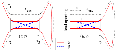
Figure 3: Detail of the small-angle self-encounter and the definitions of the various times used in the calculations. The beginning and end of the encounter region are marked by solid thin lines, the location of the Poincaré surface of section is marked by a dashed line. Each trajectory passes the Poincaré surface of section twice. Left: Small-angle self encounter fully inside the dot. Right: Small-angle self-encounter that touches the lead opening. One end of the encounter region is marked by a solid thin line, the other end is the lead opening.

Starting point of the calculation is the Landauer formula (1) together with the semiclassical expression (2) for the dot’s transmission. The pairs of classical trajectories $\alpha$ and $\beta$ that contribute to weak localization are repeated schematically in the left panel of Fig. 3, together with the definitions of the various times used in the calculation below. Following Ref. Heusler et al., 2006 (and referring there for details) we find that the weak localization correction to the transmission is equal to

$$\delta T = \frac{N_{1}N_{2}}{(N_{1}+N_{2})^{2}}\left(\prod_{j=1}^{2}\int_{0}^{\infty}\frac{d\tau_{j}}{\tau_{\rm D}}e^{-\tau_{i}/\tau_{\rm D}}\right)$$ (4)

$$\mbox{}\times\int_{0}^{\infty}d\tau_{3}e^{-\tau_{3}/\tau_{\rm D}}\int_{-c}^{c}dsdu\frac{e^{isu/\hbar-t_{{\rm enc}}/\tau_{\rm D}}}{2\pi\hbar t_{{\rm enc}}}.~{}~{}$$

Here $\tau_{1}$ and $\tau_{2}$ are the durations of the parts of the trajectories between the encounter and the lead openings and $\tau_{3}$ is the duration of the loop, see Fig. 3. The prefactor $N_{1}N_{2}/(N_{1}+N_{2})^{2}$ consists of a factor $N_{1}$ from the free sum over the incoming channel in the left contact, a factor $N_{2}/(N_{1}+N_{2})$ from the probability to escape through the right contact, and a factor $1/(N_{1}+N_{2})$ from the small-angle phase space encounter.Heusler et al. (2006) The phase space coordinates $u$ and $s$ parameterize the distance between the two parts of one of the interfering trajectories at a reference Poincaré surface of section during the self-encounter, along unstable and stable directions in phase space, respectively, see Fig. 3. The product $su$ in the exponent of Eq. (4) is the difference of the actions of the trajectories $\alpha$ and $\beta$.Spehner (2003); Turek and Richter (2003) The integration domain is the set of phase space coordinates $s$ and $u$ for which the distance between the two trajectories is smaller than a cut-off $c$, i.e., $|s|$, $|u|<c$. The cut-off $c$ is a classical scale chosen small enough that the classical dynamics can be linearized on phase space distances below $c$. The precise value of the cut-off is not relevant in the limit $\hbar\to 0$. The time $t_{{\rm enc}}$ is the duration of the encounter, i.e., the time that the two segments of the trajectories $\alpha$ and $\beta$ are within a phase-space distance $c$,

$$t_{{\rm enc}}=\frac{1}{\lambda}\ln\frac{c}{|s|}+\frac{1}{\lambda}\ln\frac{c}{|u|},$$ (5)

where $\lambda$ is the Lyapunov exponent of the classical motion inside the quantum dot. It appears in the denominator in Eq. (4) in order to cancel a spurious contribution to the integral from the freedom to choose the reference point inside the encounter region.Müller et al. (2004, 2005) The factors $\exp(-t_{{\rm enc}}/\tau_{\rm D})$ and $\exp(-\tau_{3}/\tau_{\rm D})$ are the probabilities not to escape during the encounter and during the loop segment, respectively. Although the trajectory traverses the encounter twice, the escape probability involves only one encounter duration.Rahav and Brouwer (2005a); Heusler et al. (2006)

The calculation of $\delta T$ closely follows the general principle outlined in appendix D3 of Ref. Müller et al., 2005. Limiting the integration domain to positive $u$, we first rewrite Eq. (4) as

$$\delta T=\frac{2N_{1}N_{2}\tau_{\rm D}}{(N_{1}+N_{2})^{2}}\int_{0}^{c}du\int_{-c}^{c}ds\frac{e^{-t_{{\rm enc}}/\tau_{\rm D}}\cos(su/\hbar)}{2\pi\hbar t_{{\rm enc}}}.$$ (6)

We then perform the variable change

$$u=c/\sigma,\ \ s=cx\sigma.$$ (7)

With the new integration variables, the integration domain is $-1<x<1$ and $1<\sigma<1/|x|$. Further, $t_{{\rm enc}}=\lambda^{-1}\ln(1/|x|)$. Hence, with $r=c^{2}/\hbar$, the integral (4) becomes

$$\delta T = \frac{N_{1}N_{2}r\tau_{\rm D}}{(N_{1}+N_{2})^{2}}\int_{-1}^{1}dx\frac{\cos(xr)e^{-t_{{\rm enc}}/\tau_{\rm D}}}{\pi t_{{\rm enc}}}\int_{1}^{1/|x|}\frac{d\sigma}{\sigma}$$ (8)

$$= \frac{2r\lambda\tau_{\rm D}N_{1}N_{2}}{(N_{1}+N_{2})^{2}\pi}\int_{0}^{1}dxx^{1/\lambda\tau_{\rm D}}\cos(xr)$$

$$= \frac{2N_{1}N_{2}}{(N_{1}+N_{2})^{2}\pi}\left[\lambda\tau_{\rm D}\sin r\vphantom{\int}\right.$$

$$\left.\mbox{}-r^{-1/\lambda\tau_{\rm D}}\int_{0}^{r}dxx^{1/\lambda\tau_{\rm D}}\frac{\sin x}{x}\right].$$

The term proportional to $\sin r$ is a rapidly oscillating function of Planck’s constant and is discarded in the classical limit. Writing the remaining term in terms of the Ehrenfest time,

$$\tau_{\rm E}=\frac{1}{\lambda}\ln r=\frac{1}{\lambda}\ln\frac{c^{2}}{\hbar}.$$ (9)

we find

$$\delta T=-\frac{N_{1}N_{2}}{(N_{1}+N_{2})^{2}}\frac{2}{\pi}e^{-\tau_{\rm E}/\tau_{\rm D}}\int_{0}^{r}dxx^{1/\lambda\tau_{\rm D}}\frac{\sin x}{x}.$$ (10)

The limit $\hbar\to 0$ at a fixed ratio of Ehrenfest time and dwell time consists of sending both $r=c^{2}/\hbar\to\infty$ and $\lambda\tau_{\rm D}\to\infty$. These limits can be taken independently in Eq. (10). We then find

$$\delta T=-\frac{N_{1}N_{2}}{(N_{1}+N_{2})^{2}}e^{-\tau_{\rm E}/\tau_{\rm D}}.$$ (11)

The exponential dependence of Eq. (11) is in agreement with previous calculations of the Ehrenfest-time dependence of weak localization.Adagideli (2003); Rahav and Brouwer (2005a); Brouwer and Rahav (2005); Jacquod and Whitney (2005) Note that the appearance of the classical phase-space cut-off $c$ in the definition of the Ehrenfest time does not affect the final result: In the limit $\hbar\to 0$ at fixed $\tau_{\rm E}/\tau_{\rm D}$, the dwell time $\tau_{\rm D}\to\infty$, which removes any $c$-dependence from the final expressions.

Instead of calculating the weak localization correction to the transmission, one may also calculate the quantum interference correction to the ensemble averaged reflection. Unitarity relates the total reflection $R_{i}$ off contact $i$ to the total transmission $T$,

$$R_{i}=N_{i}-T,\ \ i=1,2.$$ (12)

Although this implies $\delta R_{1}=\delta R_{2}=-\delta T$, it remains instructive to verify this result explicitly from the semiclassical formalism.

The semiclassical formula for the total reflection $R_{i}$ is the same as Eq. (2) for the total transmission $T$, but with a double sum over trajectories that connect contact $i$ to itself. The quantum correction to $R_{i}$ consists of two parts: the counterpart $\delta R_{i}^{(1)}$ of the weak localization correction to the transmission $T$, which involves encounters in the interior of the quantum dot, and an extra quantum correction $\delta R_{i}^{(2)}$ from encounters that touch the lead opening. The calculation of the first correction to $R_{i}$ only differs from the calculation of $\delta T$ in the replacement of $N_{1}N_{2}$ by $N_{i}^{2}$, $i=1,2$, so that

$$\delta R_{i}^{(1)} = -\frac{N_{i}^{2}}{(N_{1}+N_{2})^{2}}e^{-\tau_{\rm E}/\tau_{\rm D}}.$$ (13)

The calculation of the reflection correction $\delta R_{i}^{(2)}$ from encounters that touch the lead opening is a little different.Rahav and Brouwer (2006, 2005b); Jacquod and Whitney (2005) This correction is usually referred to as the ‘coherent backscattering’ correction to reflection. In the limit $\tau_{\rm E}\ll\tau_{\rm D}$, coherent backscattering can be calculated using the ‘diagonal approximation’ for the double sum over trajectories in Eq. (2).Doron et al. (1991); Lewenkopf and Weidenmüller (1991); Baranger et al. (1993a) In the diagonal approximation, only trajectories $\alpha$ and $\beta$ that are identical up to time reversal are kept. If $\tau_{\rm E}\gtrsim\tau_{\rm D}$, the diagonal approximation fails, however, and a full summation over families of trajectories very similar to the trajectory sums for weak localization is called for.Rahav and Brouwer (2005b); Jacquod and Whitney (2005)

Since the trajectories $\alpha$ and $\beta$ have the same perpendicular component of the momentum at the lead opening upon entrance as well as upon exit, the optimal choice of phase space coordinates for an encounter that touches the lead opening is a phase space coordinate $v$ that represents the perpendicular momentum at the contact, together with the unstable phase space direction $u$ (taken with respect to motion away from the contact). Note that $v$ is a meaningful coordinate for a Poincaré surface of section in an encounter that touches the lead opening, because all trajectories piercing the Poincaré surface of section exit the quantum dot together. The stable phase space coordinate $s$, which was used for small-angle self-encounters that contribute to weak localization, is not a good choice here, because in general the trajectories $\alpha$ and $\beta$ have different $s$ if the self encounter touches the lead opening. Following Refs. Spehner, 2003; Turek and Richter, 2003, we normalize $v$ such that the cross section volume element in phase space is $dudv$. With this normalization, the phase space coordinates $(u,v)$ are uniformly distributed for ergodic motion. As in the case of the calculation of the weak localization correction $\delta T$, we use the first passage of the trajectory $\alpha$ through the encounter region as a reference, consider a Poincaré surface of section at an arbitrary point during the encounter, and denote the phase space coordinates at which $\alpha$ cuts through the Poincaré surface of section a second time by $(u,v)$. The action difference $\Delta S$ is the phase space area enclosed by the four segments of the trajectories $\alpha$ and $\beta$ involved in the interference correction.Spehner (2003); Turek and Richter (2003) Recalling that $\alpha$ and its partner trajectory $\beta$ have perpendicular momenta compatible with the same modes in the lead opening, the phase space coordinates of the first and second passages of $\beta$ are $(u,0)$ and $(0,v)$, respectively, hence $\Delta S=uv$. Note that the enclosed phase space areas are conserved along the motion of the trajectories. In particular, this means that the action difference $\Delta S$ is independent of where the Poincaré surface of section is chosen and that the coordinate $v$ scales $\propto\exp(-\lambda t)$ upon moving away from the contacts.

With this, we find that the coherent backscattering correction reflection becomes

$$\delta R_{i}^{(2)} = \frac{N_{i}}{(N_{1}+N_{2})}\int d\tau_{3}e^{-\tau_{3}/\tau_{\rm D}}\int_{-c}^{c}dvdu$$ (14)

$$\mbox{}\times\int_{0}^{\lambda^{-1}\ln(c/|v|)}\frac{d\tau}{\tau_{\rm D}}\frac{e^{ivu/\hbar-t_{\rm enc}/\tau_{\rm D}}}{2\pi\hbar t_{\rm enc}},$$

where $\tau$ is the time needed to go between the Poincaré surface of section and the lead opening, see Fig. 3. The prefactor $N_{i}$ arises from the summation over the incoming transverse channel. Note that there is no additional factor $N_{i}/(N_{1}+N_{2})$ [as in the case of an encounter that resides in the interior of the quantum dot, cf. Eq. (4)], because the probability of escape through contact $i$ is unity for encounters that touch the lead opening, $i=1,2$. In Eq. (14) the encounter time is a function of $\tau$ and $u$,

$$t_{\rm enc}(\tau,u)=\tau+\lambda^{-1}\ln(c/|u|).$$ (15)

The condition $\tau<\lambda^{-1}\ln(c/|v|)$ in Eq. (14) ensures that the encounter touches the lead opening. (The precise value of the cut-off $c$ is unimportant in the limit $\hbar\to 0$, as before.) In order to perform the integrations in Eq. (14), we take $u$ to be positive and perform the variable change

$$\tau^{\prime}=\tau+\lambda^{-1}\ln(c/|u|),\ \ u=c/\sigma,\ \ v=cx\sigma.$$ (16)

With the new integration variables, the integration domain is $-1<x<1$, $1<\sigma<e^{\lambda\tau^{\prime}}$, and $0<\tau^{\prime}<\lambda^{-1}\ln(1/|x|)$. Further, $t_{{\rm enc}}=\tau^{\prime}$. Hence, with $r=c^{2}/\hbar$, the integral (14) becomes

$$\delta R_{i}^{(2)} = \frac{N_{i}\tau_{\rm D}r}{\pi(N_{1}+N_{2})}\int_{-1}^{1}dx\int_{0}^{\lambda^{-1}\ln(1/|x|)}\frac{d\tau^{\prime}}{\tau_{\rm D}}e^{-\tau^{\prime}/\tau_{\rm D}}$$

$$\mbox{}\times\int_{1}^{e^{\lambda\tau^{\prime}}}\frac{d\sigma}{\sigma\tau^{\prime}}\cos(rx)$$

$$= \frac{2N_{i}\lambda\tau_{\rm D}r}{\pi(N_{1}+N_{2})}\int_{0}^{1}dx(1-x^{1/\lambda\tau_{\rm D}})\cos(rx).$$

Neglecting terms proportional to $\sin r$, the remaining integrals are the same as for the calculation of $\delta T$, and one finds the resultRahav and Brouwer (2006, 2005b); Jacquod and Whitney (2005)

$$\delta R_{i}^{(2)}=\frac{N_{i}}{N_{1}+N_{2}}e^{-\tau_{\rm E}/\tau_{\rm D}}.$$ (18)

Adding Eqs. (13) and (18), one finds $\delta R=-\delta T$, as is required by unitarity.

III Conductance Fluctuations

The same theoretical framework can be used to calculate universal conductance fluctuations. Technically, it is most convenient to calculate the covariance of reflection coefficients $R_{1}$ and $R_{2}$ for reflection from the left and right point contacts, because it avoids the necessity of dealing with encounters that touch the two point contacts. (The case of encounters that touch the lead openings will be discussed at the end of this section.) The covariance of the reflection coefficients is directly related to the conductance variance,

$$\mbox{var}\,G=\left(\frac{2e^{2}}{h}\right)^{2}\mbox{var}\,T=\left(\frac{2e^{2}}{h}\right)^{2}\mbox{cov}\,(R_{1},R_{2}).$$ (19)

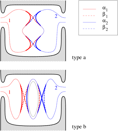
Figure 4: Two configurations of interfering trajectories that contribute to the covariance $\mbox{cov}\,(R_{1},R_{2})$ of reflection coefficients for the left and right contacts. The encounter regions, segments of the trajectories for which the phase space distance between the trajectories $1$ and $2$ is less than a classical cut-off $c$, are shown thick. In the top configuration, the trajectories $1$ and $2$ have two consecutive well-separated encounters. In the bottom panel, the trajectories $\alpha_{2}$ and $\beta_{1}$ have one more revolution around a periodic trajectory (shown dotted) than their counterparts $\alpha_{1}$ and $\beta_{2}$.

The reflections $R_{1}$ and $R_{2}$ are expressed in terms of a double sum over classical trajectories $\alpha_{i}$ and $\beta_{i}$, $i=1,2$, connecting each contact to itself, similar to the trajectory sum of Eq. (2) for the dot’s transmission. The covariance $\mbox{cov}\,(R_{1},R_{2})$ then becomes a quadruple sum over classical trajectories $\alpha_{1}$, $\beta_{1}$, $\alpha_{2}$, and $\beta_{2}$. There are two distinct configurations of four interfering trajectories that contribute to $\mbox{cov}\,(R_{1},R_{2})$, see Fig. 4. These are the counterparts for reflection of the trajectories shown in the two bottom panels of Fig. 1. We refer to them as “type a” and “type b” interfering trajectories. Other possible configurations of interfering trajectories will give contributions to $\mbox{var}\,G$ smaller by a power of $N_{1}+N_{2}$ and need not be considered in the limit $\hbar\to 0$ at fixed $\tau_{\rm E}/\tau_{\rm D}$ we consider here.Heusler et al. (2006) The configuration of Fig. 4b is not left-right symmetric and acquires an extra factor two. Denoting the contributions from interfering trajectories of types a and b as $A$ and $B$, respectively, we then have

$$\mbox{var}\,G=2\left(\frac{2e^{2}}{h}\right)^{2}(A+2B).$$ (20)

The prefactor $2$ in Eq. (20) only appears in the presence of time-reversal symmetry. It accounts for the configurations of interfering trajectories obtained by time-reversing the trajectories originating from the left contact but not the trajectories originating from the right contact.

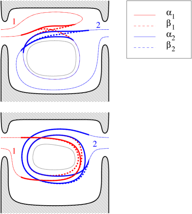
Figure 5: Two examples of interfering trajectories with overlapping encounters. The encounter regions are shown thick. In both panels, the trajectories $\beta_{1}$ and $\alpha_{2}$ have one more revolution around a closed periodic trajectory (shown dotted) than their partners $\alpha_{1}$ and $\beta_{2}$. The top panel shows two encounters that overlap at one end. This is the “three encounter” of Ref. Heusler et al., 2006. The bottom panel shows two encounters overlapping at both ends, so that the encounter region forms a closed loop. Although encounters that themselves form a closed loop do not contribute to the conductance variance if $\tau_{\rm E}\ll\tau_{\rm D}$, their contribution is essential if $\tau_{\rm E}\gg\tau_{\rm D}$.

The primary distinction between the types a and b is that the trajectories of the former type do not have segments that are close to a periodic trajectory, whereas in the latter case they do. (The periodic trajectory is the dotted loop in the right panel of Fig. 4; Here “close” means that a segment of the trajectories $\alpha$ or $\beta$ can be deformed into a periodic trajectory within the region of phase space in which the chaotic dynamics in the quantum dot can be linearized.) This means that $B$ contains all conductance fluctuations that are tied to density of states fluctuations, whereas $A$ represents the density-of-states independent fluctuations of the conductance. In the limit $\tau_{\rm E}\ll\tau_{\rm D}$ the conductance and the density of states are statistically independent,Brouwer et al. (1997) so that we expect that $B=0$ in that limit.

Although the encounters as drawn in Fig. 4 do not overlap, they can overlap in principle. In fact, such overlaps are essential for a theory of universal conductance fluctuations if the Ehrenfest time is larger than the dwell time and, hence, comparable to the total path length. Two examples of overlapping encounters are shown in Fig. 5. The top panel of Fig. 5 shows the “three-encounter” of Ref. Heusler et al., 2006. The bottom panel shows a more complicated configuration in which the two encounters overlap both at their beginning and at their end, so that the encounter region forms a closed loop. In principle, overlapping encounters can arise from bringing the two encounters of Fig. 4a close together along one of the two solid trajectories. However, as soon as the encounters of Fig. 4a overlap, one of the trajectories involved has a segment close to a periodic trajectory. Therefore, according to our definitions of the covariance contributions $A$ and $B$, the two encounters in the configuration of type a do not overlap.

Calculation of the contribution $A$ of interfering trajectories of type a is straightforward since the quantum interference correction from non-overlapping encounters factorizes,Heusler et al. (2006)

$$A=\frac{(N_{1}N_{2})^{2}}{(N_{1}+N_{2})^{4}}e^{-2\tau_{\rm E}/\tau_{\rm D}}.$$ (21)

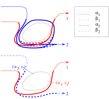
Figure 6: Top: Interfering trajectories of type b (dashed and solid curves) and the periodic trajectory (dotted). Bottom: Short versions of the interfering trajectories together with the Poincaré surfaces of section. At each Poincaré surface of section the stable and unstable phase space coordinates $s$ and $u$ parameterize the distance to the periodic trajectory.

The calculation of the contribution of interfering trajectories of type b significantly more involved. Because of the existence of configurations as shown in the bottom panel of Fig. 5, in which the encounter region winds one or several times around a periodic trajectory, one cannot calculate the contribution from trajectories of type b by considering two-encounters and three-encounters only, as was done in a previous version of this article.Brouwer and Rahav (2005) (Note, however, that since encounters that fully wind around a periodic trajectory with period $\tau_{\rm p}$ exist for periods $\tau_{\rm p}\lesssim\tau_{\rm E}$ only, considering two-encounters and three-encounters only is sufficient if $\tau_{\rm E}\ll\tau_{\rm D}$.Heusler et al. (2006) See Ref. Müller et al., 2005 for a precise calculation that verifies this for closed quantum dots.)

In order to parameterize the combinations of interfering trajectories of type b, we use coordinates that measure the phase space distance to the periodic trajectory. The periodic trajectory, as well as the four interfering trajectories of type b are shown again in the top panel of Fig. 6. The interfering trajectories consist of two “short” trajectories (trajectories $\alpha_{1}$ and $\beta_{2}$ in Fig. 4 or Fig. 6) and two “long” trajectories (trajectories $\alpha_{2}$ and $\beta_{1}$ in Fig. 4 or Fig. 6), where the long trajectories have one more revolution around the periodic trajectory than the short one. We use the two short trajectories as our reference. At a point where the phase space distance to the periodic trajectory is less than the classical cut-off $c$, for each short trajectory $i=1,2$ we draw a Poincaré surface of section and use phase space coordinates $(u_{i},s_{i})$, $i=1,2$, referring to the unstable and stable directions in phase space to describe the distance to the periodic trajectory, see Fig. 6b. Notice that we need to draw two separate Poincaré surfaces of section because the two short trajectories do not need to be within a phase space distance $c$ from the periodic trajectory at the same time. The long versions of the trajectories pass through these Poincaré surfaces of section twice and have phase space coordinates $(u_{i},s_{i}e^{-\lambda\tau_{\rm p}})$ or $(u_{i}e^{-\lambda\tau_{\rm p}},s_{i})$, $i=1,2$, where $\tau_{\rm p}$ is the period of the periodic trajectory.

In order to calculate the action difference $\Delta S=S_{\alpha_{1}}+S_{\alpha_{2}}-S_{\beta_{1}}-S_{\beta_{2}}$ we perform two successive deformations, as shown in Fig. 7. The action difference for the first deformation can be calculated using the Poincaré surface of section drawn in the top left panel of Fig. 7. The phase space coordinates of the two trajectories are $(u_{2},s_{2})$ and $(u_{1}e^{-\lambda(\tau_{\rm p}-\tau^{\prime})},s_{1}e^{-\lambda\tau^{\prime}})$, where $\tau^{\prime}$ is the time difference between the two Poincaré sections in the bottom panel of Fig. 6, measured along the periodic trajectory. Then the corresponding action difference is $(u_{2}-u_{1}e^{-\lambda(\tau_{\rm p}-\tau^{\prime})})(s_{2}-s_{1}e^{-\lambda\tau^{\prime}})$, see Refs. Spehner, 2003; Turek and Richter, 2003. The action difference for the second deformation is calculated using the Poincaré surface of section drawn in the right panel of Fig. 7. The phase space coordinates of the two trajectories involved here are $(u_{1},s_{2}e^{-\lambda(\tau_{\rm p}-\tau^{\prime})})$ and $(u_{2}e^{-\lambda\tau^{\prime}},s_{1})$, corresponding to the action difference $(u_{1}-u_{2}e^{-\lambda\tau^{\prime}})(s_{2}e^{-\lambda(\tau_{\rm p}-\tau^{\prime})}-s_{1})$. Adding the two action differences, one finds

$$\Delta S=(u_{2}s_{2}-u_{1}s_{1})(1-e^{-\lambda\tau_{\rm p}}).$$ (22)

The sign of the action difference is not relevant, as both $\Delta S$ and $-\Delta S$ appear in the final summation. Our expression for the action difference $\Delta S$ differs by a factor $1-e^{-\lambda\tau_{\rm p}}$ from the action difference used in Ref. Heusler et al., 2006. This difference is unimportant, since relevant periods $\tau_{\rm p}$ are of the order of the mean dwell time $\tau_{\rm D}$ and $\exp(-\lambda\tau_{\rm D})\ll 1$.

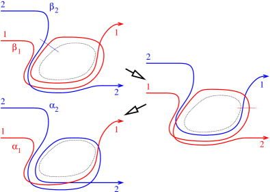
Figure 7: Two successive deformations used to calculate the action difference between the pair of trajectories in the top left diagram and the pair of trajectories in the bottom left diagram.

We count periodic trajectories that consist of several revolutions of one shorter trajectory as separate trajectories. This correctly takes into account the contribution from interfering trajectories where the difference between interfering trajectories is more than one revolution around a periodic trajectory.

Now we are ready to calculate the contribution $B$ of trajectories of type b to the reflection covariance. Repeating the steps used for the calculation of the weak localization correction $\delta T$, we find

$$B = \frac{N_{1}^{2}N_{2}^{2}}{(N_{1}+N_{2})^{4}}\left(\prod_{j=1}^{4}\int_{0}^{\infty}\frac{d\tau_{j}}{\tau_{\rm D}}e^{-\tau_{j}/\tau_{\rm D}}\right)\int d\tau_{\rm p}e^{-\tau_{\rm p}/\tau_{\rm D}}$$

$$\mbox{}\times\int_{-\tau_{\rm p}/2}^{\tau_{\rm p}/2}dt_{2}\int_{-c}^{c}ds_{1}du_{1}ds_{2}du_{2}\frac{e^{i\Delta S/\hbar-(\tau_{s}+\tau_{u})/\tau_{\rm D}}}{(2\pi\hbar)^{2}t_{\rm enc,1}t_{\rm enc,2}}.$$

Here $t_{2}$ parameterizes the point at which the Poincaré surface of section for the reflection trajectory of contact $2$ is taken, measured as the time needed to travel between the Poincaré surfaces of sections for the trajectories $1$ and $2$, see Fig. 8. The time $t_{{\rm enc},i}$ is the time during which trajectory $i$ remains within a phase space distance $c$ from the periodic trajectory, $i=1,2$. The division by $t_{{\rm enc},i}$ cancels a spurious contribution arising from the freedom to choose the Poincaré surface of section along the trajectory. The times $\tau_{s}$ and $\tau_{u}$ indicate the length of time over which the trajectories $1$ and $2$ are correlated before and after getting within a phase space distance $c$ of the closed loop, respectively, see Fig. 8. The times $\tau_{j}$, $j=1,2,3,4$, indicate the duration of the four segments of uncorrelated propagation of the two pathes when they are outside the encounter region. The classical action difference $\Delta S$ is given in Eq. (22) above.

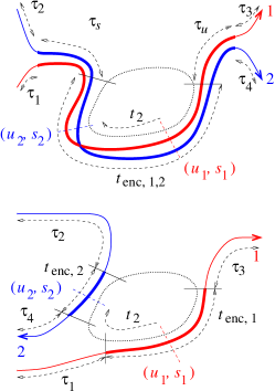
Figure 8: Definitions of the times appearing in Eq. (LABEL:eq:B). The top panel shows an example where the two short trajectories $\alpha_{1}$ and $\beta_{2}$ (solid curves) have strong correlations before and after arriving within the vicinity of the periodic trajectory (dotted curve). The time during which these strong classical correlations exist is $\tau_{s}$ or $\tau_{u}$. The bottom panel shows an example where there are no classical correlations except for the time the trajectories are in the vicinity of the periodic trajectory. In this case, $\tau_{s}=\tau_{u}=0$. In the bottom panel, the two trajectories have different encounter times $t_{{\rm enc},1}$ and $t_{{\rm enc},2}$. In the example shown in the top panel, the two encounter times $t_{{\rm enc},1}$ and $t_{{\rm enc},2}$ are (almost) equal. The thin solid lines indicate the beginning and the end of the encounter with the periodic trajectory; the total encounter regions are marked by thick trajectories. The dashed lines indicate the positions where the Poincaré surfaces of section for the two trajectories are taken.

We define the new integration variable

$$t_{2}^{\prime}=t_{2}-\lambda^{-1}\ln(c/|s_{1}|)+\lambda^{-1}\ln(c/|s_{2}|),$$ (24)

which is the time between the points where the trajectories $1$ and $2$ first come within a phase space distance $c$ from the periodic trajectory. Without loss of generality, we may assume that the phase space coordinate $s_{1}$ is positive. However, we must keep the sign of the phase space coordinate $s_{2}$ because it enters into the action difference $\Delta S$ and into the correlation time $\tau_{s}$. Making a variable change similar to that of Eq. (7),

$$s_{i}=c/\sigma_{i},\ \ u_{i}=cx_{i}\sigma_{i},\ \ i=1,2,$$ (25)

we replace the double integration $ds_{i}du_{i}$, $i=1,2$, by a single integration $dx_{i}$, $i=1,2$. This variable change cancels the denominator $t_{{\rm enc},1}t_{{\rm enc},2}$ and adds a Jacobian $(\lambda c^{2})^{2}$, where $\lambda$ is the Lyapunov exponent, see Eq. (8). We then find

$$B = \frac{N_{1}^{2}N_{2}^{2}c^{4}}{(2\pi\hbar)^{2}N^{4}}\int d\tau_{\rm p}e^{-\tau_{\rm p}/\tau_{\rm D}}I(\tau_{\rm p}),$$ (26)

with

$$I(\tau_{\rm p}) = 2\lambda^{2}\int_{-\tau_{\rm p}/2}^{\tau_{\rm p}/2}dt_{2}^{\prime}\int_{-1}^{1}dx_{1}dx_{2}\sum_{\pm}e^{-(\tau_{s}+\tau_{u})/\tau_{\rm D}}$$ (27)

$$\mbox{}\times\cos\left[r(x_{1}\mp x_{2})\right],$$

where the sign $\pm$ is the sign of $s_{2}$ and

$$r=\frac{c^{2}(1-e^{-\lambda\tau_{\rm p}})}{\hbar}.$$ (28)

The prefactor $2$ in Eq. (27) arises from fixing $s_{1}$ to be positive. Finally, we change variables $u_{1}=x_{1}$, $u_{2}=\pm x_{2}$, and $w=\pm e^{\lambda t_{2}^{\prime}}$. The integration over $t_{2}^{\prime}$ and summation over the sign $\pm$ of $s_{2}$ is then represented as the integral $\int dw/\lambda|w|$, with $e^{-\lambda\tau_{\rm p}/2}<|w|<e^{\lambda\tau_{\rm p}/2}$,

$$I(\tau_{\rm p}) = 2\lambda\int\frac{dw}{|w|}\int_{-1}^{1}du_{1}du_{2}$$ (29)

$$\mbox{}\times\cos[r(u_{1}-u_{2})]e^{-(\tau_{s}+\tau_{u})/\tau_{\rm D}}.$$

The classical limit taken here corresponds to sending $r\to\infty$, $\tau_{\rm D}\to\infty$, while keeping $\tau_{\rm E}/\tau_{\rm D}=(1/\lambda\tau_{\rm D})\ln r$ fixed. Since $I$ gets multiplied by $r^{2}\tau_{\rm D}$, see Eq. (26) above, we look for a leading contribution to $I$ of order $1/r^{2}\tau_{\rm D}$.

It is instructive to first consider the integral $I(\tau_{\rm p})$ without the factor $\exp(-\tau_{u}/\tau_{\rm D})$. Since $\tau_{s}$ does not depend on the integration variables $u_{1}$ and $u_{2}$, the integrals over $u_{1}$ and $u_{2}$ are straightforward, and one finds

$$I(\tau_{\rm p})=\frac{8\lambda}{r^{2}}\sin^{2}r\int\frac{dw}{|w|}e^{-\tau_{s}/\tau_{\rm D}}.$$ (30)

This result, however, is deceptive. The fact that $\sin^{2}r\to 1/2$ for large $r$ is an artifact of our choice of the same phase-space cut-off $c$ for the trajectories $1$ and $2$. The same artifact appears when calculating $F_{1}^{2}$ for the contribution of type a: when calculating $F_{1}$ we discarded a rapidly oscillating function $\propto\sin r$. However, the square of this rapidly oscillating function has a nonzero average which should not be retained in the final expression. We can avoid this problem by taking slightly different phase-space cut-offs for the trajectories $1$ and $2$, which amounts to replacing $\cos(ru_{1}-ru_{2}))$ by $\cos(r_{1}u_{1}-r_{2}u_{2})$. We then find

$$I=8\lambda\int\frac{dw}{|w|}\frac{\sin r_{1}\sin r_{2}}{r_{1}r_{2}}e^{-\tau_{s}/\tau_{\rm D}}.$$ (31)

In the classical limit $r_{1}$, $r_{2}\to\infty$ this is a fast oscillating function and can be discarded. By symmetry, replacing the factor $\exp(-\tau_{s}/\tau_{\rm D})$ by unity also gives a fast oscillating function which will be discarded from the final answer. Because of this, we may replace each factor $\exp(-\tau_{s,u}/\tau_{\rm D})$ by $\exp(-\tau_{s,u}/\tau_{\rm D})-1$ in the integrand of Eq. (29). After this replacement, we can restore $r_{1}=r_{2}=r$.

The fact that $I(\tau_{\rm p})=0$ without the factors $\exp(-\tau_{s}/\tau_{\rm D})$ or $\exp(-\tau_{u}/\tau_{\rm D})$ signals the statistical independence of the conductance and the density of states for a chaotic quantum dot with $\tau_{\rm E}\ll\tau_{\rm D}$.Brouwer et al. (1997) It is also crucial to ensure unitarity. Without the factors $\exp(-\tau_{s}/\tau_{\rm D})$ or $\exp(-\tau_{u}/\tau_{\rm D})$ the expression for $I(\tau_{\rm p})$ contains no reference to the phase space distance between the trajectories $1$ and $2$ at the point that they approach or leave the periodic trajectory, respectively. Without such reference, unitarity cannot be preserved, because there will be no difference between the case that the trajectories $1$ and $2$ originate/terminate at the same contact or not. With the factors $\exp(-\tau_{s}/\tau_{\rm D})$ and $\exp(-\tau_{u}/\tau_{\rm D})$ unitarity is preserved, see the discussion at the end of this section.

At this point we should specify the times $\tau_{s}$ and $\tau_{u}$. The escape of trajectories $1$ and $2$ is correlated before arriving at the closed loop only if the stable phase space coordinates $s_{1}$ and $s_{2}$ have the same sign, i.e., if $w>0$. In that case, the phase space distance between the two trajectories at the point of entrance of trajectory $1$ is $d=c|1-\exp(-\lambda t_{2}^{\prime})|=c|1-1/w|$ and the phase space distance between the two trajectories at the point of entrance of trajectory $2$ is $d=c|\exp(\lambda t_{2}^{\prime})-1|=c|w-1|$. Note that for $w$ close to $1$ (which is when escape correlations are relevant) the two phase space distances are equal. For definiteness, and in order to have an assignment that is symmetric under the exchange $1\leftrightarrow 2$, we use the largest of these two phase space distances in the following considerations. Hence, if $w>1$, we have $d=c(w-1)$, whereas $d=c(1/w-1)$ if $0<w<1$. The correlation time (if positive), then, follows from setting $de^{\lambda\tau_{s}}=c(b-1)$, where $e^{\lambda\tau_{\rm p}/2}>b>1$ is a suitably chosen number of order unity,

$$\tau_{s}=\left\{\begin{array}[]{ll}\lambda^{-1}\ln[(b-1)/(w-1)]&\mbox{if $1<w<b$},\\ \lambda^{-1}\ln[(b-1)/(1/w-1)]&\mbox{if $1/b<w<1$},\\ 0&\mbox{otherwise}.\end{array}\right.$$ (32)

The final results will be independent of the choice of the cut-off $b$.

The definition of the correlation time $\tau_{u}$ is similar. Proceeding as before, one finds that $\tau_{u}$ depends on the product $z=wu_{1}/u_{2}$: this encodes both the time difference between the exit points of trajectories $1$ and $2$ and the sign of the unstable phase space coordinates at those points. There is one subtlety when regarding escape for the exiting trajectories: if $|z|<e^{-\lambda\tau_{\rm p}/2}$ or $|z|>e^{\lambda\tau_{\rm p}/2}$, $|z|$ has to be brought back to the range $e^{-\lambda\tau_{\rm p}/2}<|z|<e^{\lambda\tau_{\rm p}/2}$ by multiplication with the appropriate number of factors of $e^{\pm\lambda\tau_{\rm p}}$. This procedure takes into account that the trajectories $1$ and $2$ can make different numbers of revolutions around the closed loop before exiting. (There was no such complication when considering $\tau_{s}$, because the integration domain for $w$ is $e^{-\lambda\tau_{\rm p}/2}<|w|<e^{\lambda\tau_{\rm p}/2}$.)

Since $\tau_{s}$ and $\tau_{u}$ appear in the combination $\exp(-\tau_{s,u}/\tau_{\rm D})$ only, we write $\exp(-\tau_{s}/\tau_{\rm D})=f(w)$, $\exp(-\tau_{u}/\tau_{\rm D})=f(z)$. We then have $f(x)=1$ if $x<0$,

$$f(x)=\left(\frac{x-1}{b-1}\right)^{1/\lambda\tau_{\rm D}}\ \ \mbox{if $1<x<b$},$$ (33)

and $f(x)=1$ if $b<x<e^{\lambda\tau_{\rm p}/2}$. Further,

$$f(x)=f(1/x)\ \ \mbox{and}\ \ f(x)=f(xe^{\lambda\tau_{\rm p}}).$$ (34)

Note that the function $f$ is continuous and piecewise differentiable. Also notice that $f=1$ except in the case of strong classical correlations between the trajectories $1$ and $2$.

With this choice of the function $f(z)$, we find that the integral $I(\tau_{\rm p})$ reads

$$I = \frac{4\lambda}{r}\int\frac{dw}{w}[f(w)-1]\int_{0}^{1}du\left\{\int_{-|w|}^{|w|}dz[f(z)-1]\frac{\partial}{\partial z}\sin[ur(z/w-1)]+\int_{-1/|w|}^{1/|w|}dz[f(z)-1]\frac{\partial}{\partial z}\sin[ur(zw-1)]\right\}.$$

Since $f(w)=1$ if $w<1/b$ or $w>b$, we can restrict the integration range for $w$ to $1/b<w<b$. Performing a partial integration to $z$, we have

$$I = -\frac{4\lambda}{r}\int_{1/b}^{b}\frac{dw}{w}[f(w)-1]\int_{0}^{1}du\left\{\int_{-w}^{w}dz\frac{\partial f(z)}{\partial z}\sin[ur(z/w-1)]+\int_{-1/w}^{1/w}dz\frac{\partial f(z)}{\partial z}\sin[ur(zw-1)]\right\}.$$ (36)

For the $z$ integration in the second line, there will be contributions from the regions $1/b<z<w$ and $e^{-n\lambda\tau_{\rm p}}/b<z<e^{-n\lambda\tau_{\rm p}}b$, $n=1,2,\ldots$. For the $z$ integration in the third line, there will be contributions from the regions $1/b<z<1/w$, $e^{-n\lambda\tau_{\rm p}}/b<z<e^{-n\lambda\tau_{\rm p}}b$, $n=1,2,\ldots$. In the region $1/b<z<b$ one has

$$\frac{\partial f(z)}{\partial z} = \frac{1}{(z-1)\lambda\tau_{\rm D}}f(z)\ \ \mbox{if $z>1$},$$

$$\frac{\partial f(z)}{\partial z} = \frac{1}{z(z-1)\lambda\tau_{\rm D}}f(z)\ \ \mbox{if $z<1$}.$$ (37)

Focusing on the integration range $1/b<z<b$, we then find

$$I = \frac{8}{r\tau_{\rm D}}\int_{1}^{b}\frac{dw}{w}\int_{1}^{w}\frac{dz}{z-1}[f(w)-1]f(z)\int_{0}^{1}du\left\{\sin[ru(1/zw-1)]-\sin[ru(z/w-1)]\right\}$$ (38)

$$\mbox{}+\frac{8}{r\tau_{\rm D}}\int_{1}^{b}\frac{dw}{w-1}\int_{1}^{w}\frac{dz}{z}[f(z)-1]f(w)\int_{0}^{1}du\left\{\sin[ru(1/zw-1)]+\sin[ru(z/w-1)]\right\}.$$

Although these integrals can be evaluated for general $b$, the evaluation is simplest if $b-1\ll 1$ (but still $b-1$ of order unity). Writing $z=1+(b-1)\zeta/u$ and $w=1+(b-1)\xi/u$ and expanding in $b-1$, one finds

$$I = -\frac{16(b-1)}{r\tau_{\rm D}}\int_{0}^{1}d\xi\int_{0}^{1}\frac{d\zeta}{\zeta}\int_{\max(\xi,\zeta)}^{1}\frac{du}{u}[(\xi/u)^{1/\lambda\tau_{\rm D}}-1](\zeta/u)^{1/\lambda\tau_{\rm D}}\cos[r(b-1)\xi]\sin[r(b-1)\zeta].$$ (39)

Performing the integral over $u$ followed by a partial integration over $\xi$, the limit $r\to\infty$ at fixed ratio $\tau_{\rm E}/\tau_{\rm D}=(1/\lambda\tau_{\rm D})\ln r$ can be taken. One then finds

$$I=2\pi^{2}(1-r^{-2/\lambda\tau_{\rm D}})/r^{2}\tau_{\rm D}.$$ (40)

There is an alternative (and more intuitive) derivation of Eq. (39) if we restrict our attention to interfering trajectories that arrive at and depart from the periodic trajectory at (classically) close phase space points from the very start of the calculation. This is the situation drawn in the top panel of Fig. 8. Instead of choosing the Poincaré surfaces of section at an arbitrary point during the encounter with the periodic trajectory, we may choose them at the beginning and end of the encounter with the periodic trajectory (indicated by the thin solid lines in the top panel of Fig. 8). At the first (entrance) Poincaré surface of section, we use the unstable phase space coordinate $u$ measured with respect to the periodic trajectory, and the difference $s^{\prime}$ of the stable phase space coordinates of the trajectories $\alpha_{1}$ and $\beta_{2}$. (Since these trajectories depart from the periodic trajectory together, their unstable phase space coordinate can be considered equal at this Poincaré surface of section.) Similarly, at the second (exit) Poincaré surface of section, we use the common stable phase space coordinate $s$ of both trajectories, measured with respect to the periodic trajectory, together with the difference $u^{\prime}$ of the unstable phase space coordinates. The total time the trajectory $\alpha_{1}$ spends near the periodic trajectory is $\lambda^{-1}\ln(c/|u|)=\lambda^{-1}\ln(c/|s|)$, hence $|s|=|u|$. In terms of these coordinates, $\exp(-\tau_{s}/\tau_{\rm D})=|s^{\prime}/c(b-1)|^{1/\lambda\tau_{\rm D}}$ and $\exp(-\tau_{u}/\tau_{\rm D})=|u^{\prime}/c(b-1)|^{1/\lambda\tau_{\rm D}}$. Fixing the positions of the Poincaré surfaces of section gives a Jacobian $\lambda c|u|$ and eliminates the factor $t_{{\rm enc},1}t_{{\rm enc},2}$ from the denominator in Eq. (LABEL:eq:B).Müller et al. (2005) Upon dividing all coordinates by the phase space cut-off $c$, we then find

$$I = 4\lambda\int_{1-b}^{b-1}ds^{\prime}du^{\prime}\int_{0}^{1}duu(|s^{\prime}/(b-1)|^{1/\lambda\tau_{\rm D}}-1)$$ (41)

$$\mbox{}\times(|u^{\prime}/(b-1)|^{1/\lambda\tau_{\rm D}}-1)\cos[ur(s^{\prime}-u^{\prime})],$$

where we added factors $2$ for the signs of $u$ and $s$. Rewriting the integrals such that the integrations over $s^{\prime}$ and $u^{\prime}$ are all between $0$ and $b-1$ and performing a partial integration to $s^{\prime}$ we find

$$I = -\frac{16}{\tau_{\rm D}r}\int_{0}^{b-1}\frac{ds^{\prime}}{s^{\prime}}du^{\prime}\int_{0}^{1}du(|u^{\prime}/(b-1)|^{1/\lambda\tau_{\rm D}}-1)$$ (42)

$$\mbox{}\times|s^{\prime}/(b-1)|^{1/\lambda\tau_{\rm D}}\sin(urs^{\prime})\cos(uru^{\prime}).$$

Upon shifting variables $s^{\prime}=\zeta(b-1)/u$ and $u^{\prime}=\xi(b-1)/u$ one then arrives at Eq. (39) above.

The $z$ integrations with $1/b<ze^{n\tau\lambda}<b$ with $n=1$, $2$, … do not give a contribution to $I(\tau_{\rm p})$ in the limit $r\to\infty$. This can be seen by noting that all oscillating integrals all contain fast oscillating phases proportional to $r(1-e^{-n\lambda\tau_{\rm p}})$.

Putting everything together, we find

$$B=\frac{N_{1}^{2}N_{2}^{2}}{2(N_{1}+N_{2})^{4}\tau_{\rm D}}\int d\tau_{\rm p}\frac{e^{-\tau_{\rm p}/\tau_{\rm D}}}{(1-e^{-\lambda\tau_{\rm p}})^{2}}(1-e^{-2\tau_{\rm E}/\tau_{\rm D}}).$$ (43)

Setting a lower cut-off for the $\tau_{\rm p}$-integration at $\tau_{\rm p}\gtrsim 1/\lambda$ and taking the limit $\tau_{\rm D}\lambda\gg 1$, we finally arrive at the simple result

$$B=\frac{N_{1}^{2}N_{2}^{2}}{2(N_{1}+N_{2})^{4}}(1-e^{-2\tau_{\rm E}/\tau_{\rm D}}).$$ (44)

Substitution into Eq. (20) then gives

$$\mbox{var}\,G=2\left(\frac{2e^{2}}{h}\right)^{2}\frac{N_{1}^{2}N_{2}^{2}}{(N_{1}+N_{2})^{4}}.$$ (45)

Equation (45) is the main result of this article. The variance of the conductance is independent of the Ehrenfest time. Equation (45) was derived for a quantum dot without an applied magnetic field. With a magnetic field strong enough to fully break time-reversal symmetry $\mbox{var}\,G$ is reduced by a factor two.

The most remarkable feature of Eq. (45) is that the conductance fluctuations survive in the limit $\tau_{\rm E}\gg\tau_{\rm D}$. The particular classical trajectories that give rise to conductance fluctuations in this limit can be identified by inspection of the calculation above. The constant term in Eq. (45) can be traced back to the lower limit on the $u$ integration in Eq. (39) which, in turn, results from trajectories that wind many times around the periodic trajectory. Although such trajectories must spend a time $\gtrsim\tau_{\rm E}$ inside the quantum dot in order to contribute to the conductance fluctuations, their survival probability depends on the period $\tau_{\rm p}$ of the periodic trajectory only, not on the actual time they spend inside the quantum dot.

Instead of calculating the conductance variance through the covariance of the reflection off the two contacts, one can also directly calculate the variance of the conductance or the variance of the reflection. As in the case of the calculation of the quantum correction to the average conductance, there are two types of contributions to the fluctuations: interfering trajectories for which all encounters lie within the interior of the quantum dot and interfering trajectories for which at least one encounter touches the lead opening. The calculation of the first type, all encounters inside the quantum dot, proceeds in essentially the same was as the calculation of the reflection covariance outlined above. Below, we discuss how the above calculations should be modified to include the second type, for which one or more encounters touch the lead opening. We find that, once encounters that touch the lead opening are taken into account, unitarity is obeyed for contributions of type a and b separately.

For trajectories of type a, there are two encounters that each can be close to a lead opening. For each encounter, however, the configuration of trajectories is identical to that of coherent backscattering calculation. Repeating the steps of the last part of the previous section, verification of unitarity is immediate.

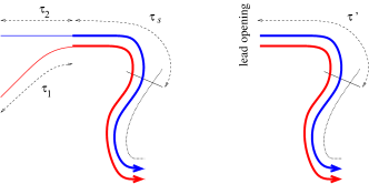
Figure 9: Comparison of a part of a type b encounter that fully resides inside the quantum dot (left) and an encounter that touches to lead opening (right). The relevant segments of the (short) trajectories $\alpha_{1}$ and $\beta_{2}$ are shown solid, the periodic trajectory is shown dotted.

For trajectories of type b, a schematic drawing showing the difference between an encounter that fully resides inside the quantum dot and an encounter that touches the lead opening is shown in Fig. 9. For an encounter that touches the lead opening, one replaces the phase space coordinate differences $s^{\prime}$ or $u^{\prime}$ in Eq. (41) by $v$, where $v$ represents the perpendicular component of the momentum in the lead opening. As in Sec. II, we normalize $v$ such that the volume element in phase space is $dudv$. With this choice of phase space coordinates, the action difference for two pairs of trajectories involved in an encounter that resides inside the quantum dot is the same as the action difference for two pairs of trajectories for which one of the encounter extends to the lead opening, up to the substitution $s^{\prime}\to v$ or $u^{\prime}\to v$. One then obtains the contribution of encounters that touch the lead opening by making the replacement

$$\frac{N_{i}}{N_{1}+N_{2}}\left(\prod_{j=1}^{2}\int_{0}^{\infty}\frac{d\tau_{j}}{\tau_{\rm D}}e^{-\tau_{j}/\tau_{\rm D}}\right)e^{-\tau_{s,u}/\tau_{\rm D}}$$ (46)

$$\to \int_{0}^{\tau_{v}}\frac{d\tau^{\prime}}{\tau_{\rm D}}e^{-\tau^{\prime}/\tau_{\rm D}}~{}~{}~{}~{}~{}~{}~{}~{}~{}~{}~{}~{}~{}~{}~{}~{}~{}~{}~{}~{}~{}~{}~{}$$

in the expression for the correlator with encounters that reside inside the quantum dot only. Here $\tau^{\prime}$ is the travel time between the lead opening and the point where the two trajectories get close to the periodic trajectory and $\exp(-\tau_{v}/\tau_{\rm D})=|v/c(b-1)|^{1/\lambda\tau_{\rm D}}$. The $\tau^{\prime}$ integration gives a factor $1-e^{-\tau_{v}/\tau_{\rm D}}$, so that the remaining integrals are the same as for the case that all encounters are inside the quantum dot and one verifies that unitarity is obeyed for type b encounters as well.

IV Time dependence

Although the calculation of the previous section answers the question which trajectories are responsible for the conductance fluctuations in the limit of large Ehrenfest times — trajectories that wind many times around a certain periodic trajectory —, it does not tell us how long these trajectories spend inside the quantum dot. That question can be answered by adding an imaginary term to the energy. Such an imaginary term gives rise to an additional exponential decay $\exp(-t_{\alpha}/2\tau_{\rm abs})$ for each trajectory $\alpha$, where $t_{\alpha}$ is the total duration of trajectory $\alpha$ and $\tau_{\rm abs}$ is the corresponding absorption time. A minimal time needed for quantum interference shows up through an exponential dependence on $1/\tau_{\rm abs}$. In the calculations below, we keep the ratios $\tau_{\rm E}/\tau_{\rm D}$ and $\tau_{\rm E}/\tau_{\rm abs}$ fixed while taking the classical limit $\hbar\to 0$.

The addition of absorption has been used in the numerical simulations of Refs. Tworzydlo et al., 2004c; Rahav and Brouwer, 2005a, 2006 as a diagnostic tool to investigate the microscopic mechanism of quantum interference corrections. Reference Rahav and Brouwer, 2006 found that the difference between weak localization and conductance fluctuations not only concerned the dependence of their magnitude on the Ehrenfest time — exponential decay versus independence of the Ehrenfest time —, but also the minimal dwell time of trajectories that contribute to quantum interference. According to the numerical simulations, the minimal dwell time for weak localization is $2\tau_{\rm E}$, whereas the minimal dwell time of trajectories contributing to conductance fluctuations was found to be $\tau_{\rm E}$. Below we show that this observation is fully consistent with the semiclassical theory.

We first consider weak localization. With the imaginary term added to the energy, one finds that the quantum correction to the transmission is given by

$$\delta T = \frac{N_{1}N_{2}}{(N_{1}+N_{2})^{2}}\left(\prod_{j=1}^{2}\int_{0}^{\infty}\frac{d\tau_{j}}{\tau_{\rm D}}e^{-\tau_{j}/\tau_{\rm D}-\tau_{j}/\tau_{\rm abs}}\right)$$ (47)

$$\mbox{}\times\int d\tau_{3}e^{-\tau_{3}/\tau_{\rm D}-\tau_{3}/\tau_{\rm abs}}$$

$$\mbox{}\times\int_{-c}^{c}dsdu\frac{e^{isu/\hbar-t_{\rm enc}/\tau_{\rm D}-2t_{\rm enc}/\tau_{\rm abs}}}{2\pi\hbar t_{\rm enc}}.$$

Note the factor two in front of $t_{\rm enc}/\tau_{\rm abs}$ in the survival probability during the encounter. This factor two arises because trajectories that contribute to weak localization travel the encounter region twice. Performing the integrations as in Sec. II, one finds

$$\delta T=-\frac{N_{1}N_{2}}{(N_{1}+N_{2})^{2}}\frac{\left(1+2\tau_{\rm D}/\tau_{\rm abs}\right)}{\left(1+\tau_{\rm D}/\tau_{\rm abs}\right)^{3}}e^{-\tau_{\rm E}/\tau_{\rm D}-2\tau_{\rm E}/\tau_{\rm abs}}.$$ (48)

Similarly, for reflection one finds

$$\delta R_{i} = \frac{N_{1}N_{2}}{(N_{1}+N_{2})^{2}}\frac{\left(1+2\tau_{\rm D}/\tau_{\rm abs}\right)}{\left(1+\tau_{\rm D}/\tau_{\rm abs}\right)^{3}}e^{-\tau_{\rm E}/\tau_{\rm D}-2\tau_{\rm E}/\tau_{\rm abs}}$$

$$\mbox{}+\frac{N_{i}}{N_{1}+N_{2}}\frac{(\tau_{\rm D}/\tau_{\rm abs})^{2}}{\left(1+\tau_{\rm D}/\tau_{\rm abs}\right)^{3}}e^{-\tau_{\rm E}/\tau_{\rm D}-2\tau_{\rm E}/\tau_{\rm abs}}.$$

In the limit $\tau_{\rm E}\ll\tau_{\rm D}$, $\tau_{\rm abs}$ these results agree with those obtained from random matrix theory.Brouwer and Beenakker (1997) Note that $\delta R_{i}$ no longer equals $-\delta T$, $i=1,2$, in the presence of absorption.

The exponential dependence $\propto\exp(-2\tau_{\rm E}/\tau_{\rm abs})$ indicates that the minimal duration of a trajectory that contributes to weak localization is $2\tau_{\rm E}$: a self-encounter lasts one Ehrenfest time and each trajectory to weak localization passes through the encounter region twice. The fact that the dwell time dependence $\propto\exp(-\tau_{\rm E}/\tau_{\rm D})$ does not have this factor two is a result of classical correlations between the two segments of the trajectory that pass through the encounter region.Rahav and Brouwer (2005a); Heusler et al. (2006) Both effects — the minimal time $2\tau_{\rm E}$ needed for weak localization and the exponential suppression $\propto\exp(-\tau_{\rm E}/\tau_{\rm D})$ are consistent with the numerical simulations of Refs. Rahav and Brouwer, 2005a, 2006.

For the conductance fluctuations we treat the contributions of trajectories of types a and b separately. We limit our discussion to the covariance $\operatorname{cov}(R_{1},R_{2})$ of the reflections off the two point contacts. Including absorption into the covariance contribution $A$ of trajectories of type a, one finds

$$A=\frac{(N_{1}N_{2})^{2}}{(N_{1}+N_{2})^{4}}\frac{\left(1+2\tau_{\rm D}/\tau_{\rm abs}\right)^{2}}{(1+\tau_{\rm D}/\tau_{\rm abs})^{6}}e^{-2\tau_{\rm E}/\tau_{\rm D}-4\tau_{\rm E}/\tau_{\rm abs}}.$$ (50)

In order to calculate the contribution of trajectories of type b, we need to calculate the integral $I(\tau_{\rm p})$ in the presence of absorption,

$$I(\tau_{\rm p}) = 2\lambda e^{-\tau_{\rm p}/\tau_{\rm abs}}\int\frac{dw}{|w|}\int_{-1}^{1}du_{1}du_{2}|u_{1}u_{2}|^{1/\lambda\tau_{\rm abs}}$$

$$\mbox{}\times\cos(r_{1}u_{1}-r_{2}u_{2})e^{-(\tau_{s}+\tau_{u})(1/\tau_{\rm D}+2/\tau_{\rm abs})}.$$

Here we used that the time the short trajectories spend near the periodic trajectory is $\lambda^{-1}\ln(1/|u_{i}|)$, $i=1,2$, and that the time spent by the long trajectory is $\tau_{\rm p}+\lambda^{-1}\ln(1/|u_{i}|)$. As before, we first calculate $I$ without the exponential factors involving $\tau_{s}$ or $\tau_{u}$. We then find

$$I(\tau_{\rm p})=\frac{4\pi^{2}\tau_{\rm p}}{r^{2}\tau_{\rm abs}^{2}}e^{-\tau_{\rm p}/\tau_{\rm abs}-2\tau_{\rm E}/\tau_{\rm abs}}.$$ (52)

Replacing one exponential factor $\exp[-\tau_{s,u}(1/\tau_{\rm D}+2/\tau_{\rm abs})]$ by $\exp[-\tau_{s,u}(1/\tau_{\rm D}+2/\tau_{\rm abs})]-1$ while still setting $\tau_{u,s}=0$ in the other exponential factor, one finds no significant contribution to $I$. Hence, the remaining contribution to $I$ can be calculated by replacing both factors $\exp[-\tau_{s,u}(1/\tau_{\rm D}+2/\tau_{\rm abs})]$ by $\exp[-\tau_{s,u}(1/\tau_{\rm D}+2/\tau_{\rm abs})]-1$. The result then follows from Eq. (39) after addition of a factor $u^{2/\lambda\tau_{\rm abs}}$ and replacement of $1/\tau_{\rm D}$ by $1/\tau_{\rm D}+2/\tau_{\rm abs}$. Performing the integrals as described in Sec. III, we find

$$I(\tau_{\rm p}) = \frac{4\pi^{2}\tau_{\rm p}}{r^{2}\tau_{\rm abs}^{2}}e^{-\tau_{\rm p}/\tau_{\rm abs}-2\tau_{\rm E}/\tau_{\rm abs}}$$ (53)

$$\mbox{}+\frac{2\pi^{2}(1/\tau_{\rm D}+2/\tau_{\rm abs})^{2}}{r^{2}(1/\tau_{\rm D}+1/\tau_{\rm abs})}e^{-\tau_{\rm p}/\tau_{\rm abs}}$$

$$\mbox{}\times\left[e^{-2\tau_{\rm E}/\tau_{\rm abs}}-e^{-2\tau_{\rm E}/\tau_{\rm D}-4\tau_{\rm E}/\tau_{\rm abs}}\right].$$

Adding the contributions of trajectories of types a and b, the final result becomes

$$\operatorname{cov}(R_{1},R_{2}) = \frac{(N_{1}N_{2})^{2}}{(N_{1}+N_{2})^{4}}e^{-2\tau_{\rm E}/\tau_{\rm abs}}$$

$$\mbox{}\times\frac{(1+2\tau_{\rm D}/\tau_{\rm abs})^{2}+2(\tau_{\rm D}/\tau_{\rm abs})^{2}}{(1+\tau_{\rm D}/\tau_{\rm abs})^{6}}.$$

The limit $\tau_{\rm E}/\tau_{\rm D}\to 0$ agrees with the result obtained from random matrix theory.Brouwer and Beenakker (1997) The exponential decay $\propto\exp(-2\tau_{\rm E}/\tau_{\rm D})$ corresponds to a minimal dwell time $\tau_{\rm E}$ for trajectories that contribute to conductance fluctuations. This is consistent with the numerical simulations of Refs. Tworzydlo et al., 2004c and Rahav and Brouwer, 2006. The same conclusion remains true for other correlators of transmissions and reflections (which need not be equal to $\mbox{cov}\,(R_{1},R_{2})$ in the presence of absorption).

V Conclusion

In the previous sections, we have calculated the Ehrenfest-time dependence of the weak localization correction and the conductance fluctuations of a ballistic quantum dot with ideal point contacts, using a trajectory-based semiclassical theory. We find that the Ehrenfest-time dependences of weak localization and conductance fluctuations are remarkably different: whereas weak localization is suppressed exponentially if the Ehrenfest time $\tau_{\rm E}$ is much larger than the mean dwell time $\tau_{\rm D}$, the conductance fluctuations are independent of the ratio $\tau_{\rm E}/\tau_{\rm D}$. Our calculation explains the numerical simulations of the conductance fluctuations in Refs. Tworzydlo et al., 2004b; Jacquod and Sukhorukov, 2004.

The numerical observation of Ehrenfest-time independent conductance fluctuations was remarkable, because trajectories need to remain inside the quantum dot during at least a time $\tau_{\rm E}$ if they are to contribute to quantum interference corrections, so that one expects that interference corrections to the conductance should disappear if $\tau_{\rm E}\gg\tau_{\rm D}$. Our calculation shows that the latter expectation is not always born out. The Ehrenfest-time independent contribution to the conductance fluctuations we find here arises from pairs of trajectories that wind many times around a periodic trajectory. On the one hand, such configurations of interfering trajectories have sufficient duration to allow for small action differences and thus provide a significant quantum interference correction. On the other hand, they are not as much affected by classical escape into the leads: The survival probability depends on the period of the periodic trajectory involved, not on the Ehrenfest time.

In Refs. Tworzydlo et al., 2004b and Jacquod and Sukhorukov, 2004 the ‘effective random matrix theory’ of Silvestrov et al.Silvestrov et al. (2003) was used to explain the numerical observation of Ehrenfest-time independent conductance fluctuations. According to the effective random matrix theory, phase space is separated into a ‘classical part’, corresponding to all trajectories with dwell time less than the Ehrenfest time, and a ‘quantum part’, which has all trajectories with dwell time larger than $\tau_{\rm E}$. The wave nature of the electrons plays no role in the classical part of phase space, whereas the quantum part of phase space is described using random matrix theory. The effective random matrix theory was able to correctly describe the Ehrenfest-time dependence of shot noiseTworzydlo et al. (2003) and the density of states of an Andreev quantum dot,Silvestrov et al. (2003); Beenakker (2005); Goorden et al. (2005) but it missed the Ehrenfest-time dependence of weak localization.Rahav and Brouwer (2005a) According to our semiclassical theory, the effective random matrix theory not only gave the correct magnitude of the universal conductance fluctuations, but it also gives the right dependence on an imaginary potential.Tworzydlo et al. (2004c) While it is understood that the effective random matrix theory is not a comprehensive theory of the Ehrenfest time dependence of quantum transport, it remains an interesting question to classify which transport phenomena are described by this phenomenological theory and which are not.