Transport through a double barrier for interacting quasi one-dimensional electrons in a Quantum Wire in the presence of a transverse magnetic field

Abstract

We discuss the Luttinger Liquid behaviour of a semiconducting Quantum Wire. We show that the measured value of the bulk critical exponent, $\alpha_{bulk}$, for the tunneling density of states can be easily calculated.

Then, the problem of the transport through a Quantum Dot formed by two Quantum Point Contacts along the Quantum Wire, weakly coupled to spinless Tomonaga-Luttinger liquids is studied, including the action of a strong transverse magnetic field $B$. The known magnetic dependent peaks of the conductance, $G(B)$, in the ballistic regime at a very low temperature, $T$, have to be reflected also in the transport at higher $T$ and in different regimes. The temperature dependence of the maximum $G_{max}$ of the conductance peak, according to the Correlated Sequential Tunneling theory, yields the power law $G_{max}\propto T^{2\alpha_{end}-1}$, with the critical exponent, $\alpha_{end}$, strongly reduced by $B$.

This behaviour suggests the use of a similar device as a magnetic field modulated transistor.

I Introduction

Progress in semiconductor device fabrication and carbon technology allowed for the construction of several low-dimensional structures at the nanometric scale, and many novel transport phenomena have been revealed.

The electron-electron (e-e) correlation effects, usually negligible in three-dimensional devices, attract considerable interest, because of the dominant role which they play in one dimension, by determining the physical properties of a one dimensional (1D) metal.

The main consequence of the e-e Coulomb repulsive interaction in 1D systems of interacting electrons is the formation of a Tomonaga-Luttinger liquid (TLl) with properties that are dramatically different from the ones of usual metals with a Fermi liquid of electronsegg ; TL ; TLreviwew .

Because of the e-e interaction, in the TLl Landau quasiparticles are unstable and the low-energy excitation is achieved by exciting an infinite number of plasmons (collective electron-hole pair modes), making the transport intrinsically different from that of a Fermi liquid. Hence, it follows a power-law dependence of physical quantities, such as the tunneling density of states (TDOS), as a function of the energy or the temperature.

Transport in 1D - Thus, the transport through 1D devices attracts considerable interest, because it displays a power-law zero-bias anomaly (ZBA) for the conduction. The tunneling conductance, $G$, reflects the power law dependence of the DOS in a small bias experimentkf

$$G=dI/dV\propto T^{\alpha_{bulk}},$$ (1)

for $eV_{b}\ll k_{B}T$, where $V_{b}$ is the bias voltage, $T$ is the temperature and $k_{B}$ is Boltzmann’s constant. Many theoretical works and experiments, during the last decade, concentrated on the power-law behavior of the electron tunneling by analyzing quantum Hall edge systems kf ; wen ; fn , carbon nanotubes (CNs)cnts ; tubes , and semiconductor Quantum Wires (QWs)tarucha ; yacoby .

The bulk critical exponent can be obtained in several different waysTLreviwew and has the form

$$\alpha_{bulk}=\frac{1}{4}\left(K+\frac{1}{K}-2\right).$$ (2)

If we follow the RG approach noi ; noia1 ; noia2 for the unscreened e-e interaction we obtain

$$\sqrt{1+\frac{U_{0}(q_{c},B)}{(2\pi{v}_{F})}}=\frac{1}{K},$$ (3)

where $v_{F}$ is the Fermi velocity and $U_{0}(p,B)$ corresponds to the Fourier transform of the 1D e-e interaction potential, also depending on the magnetic field $B$. Thus $K$ is a function of the interaction strength ($K<1$ corresponding to repulsive interaction) while $q_{c}=2\pi/L$ is the natural infrared cut-off depending on the longitudinal length of the quasi 1D device.

The power-law behaviour characterizes also the thermal dependence of $G$ when an impurity is present along the 1D devices. The theoretical approach to the presence of obstacles mixes two theories corresponding to the single particle scattering and the TLl theory of interacting electrons. In fact the presence of a barrier is usually modeled by a potential barrier $V_{B}({\bf r})$ and the single particle scattering gives the transmission, probability, $|t|^{2}$, depending in general on the single particle energy $\varepsilon$. Following ref.sh , we can proceed to the RG analysis which, in the limit of Strong Barrier, gives the conductance, $G$, as a function of the temperature and $|t|$ i.e.

$$G\propto|t(\varepsilon,T)|^{2}\equiv|t(\varepsilon)|^{2}T^{2\alpha_{end}.}$$ (4)

Here we introduced a second critical exponent,

$$\alpha_{end}=(1/K-1),$$ (5)

also depending on $K$.

ExperimentsPostma01 ; Bozovic01 show transport through an intrinsic quantum dot (QD) formed by a double barrier within a 1D electron system, allowing for the study of the resonant or sequential tunneling. The linear conductance typically displays a sequence of peaks, when the gate voltage, $V_{g}$, increases. Since the initial theoretical work on this topic,kf ; kf2 ; Furusaki the double-barrier problem in the absence of a magnetic field in a TLl has attracted a significant amount of attention among theorists.Sassetti95 ; Furusaki98 ; Braggio00 ; Thorwart02 ; Nazarov03 ; Polyakov03 ; Komnik03 ; Hugle04 The 1D nature of the correlated electrons is responsible for the differences with respect to the quantum Coulomb blockade theory for conventional, e.g., semiconducting QDs [13] . In the (Uncorrelated) Sequential Tunneling (UST) approximation the temperature dependence of the maxima of those peaks follows the power law Furusaki98

$$G_{max}\propto T^{\alpha_{end}-1},$$ (6)

with $\alpha_{end}$ being the DOS exponent for tunneling into the end of a TLl. However, recent experiments Postma01 suggest a different power law

$$G_{max}\propto T^{\alpha_{end-end}-1},$$ (7)

with $\alpha_{end-end}=2\alpha_{end}$. This result follows from the Correlated Sequential Tunneling (CST) theory typical for tunneling between the ends of two TLls.

Quasi 1D devices - Semiconductor QWs are quasi 1D devices (having a width smaller than $1000\AA$thor and a length of some microns), where the electron waves are in some ways analogous to electromagnetic waves in waveguides. In these devices the electrons are confined to a narrow 1D channel, with the motion perpendicular to the channel quantum mechanically frozen out. Such wires can be fabricated using modern semiconductor technologies, such as electron beam lithography and cleaved edge overgrowth.

QWs are usually made at the interface of different thin semiconducting layers (typically $GaAs:AlGaAs$) heterojunction, where a quasi two dimensional electron gas (2DEG) can be formed by etching the heterojunction thor .

In a recent experimentqw1 on long nanowires of degenerate semiconductor $InSb$ (with a diameter around $50\AA$ and a length of $0.1-1$ mm) a zero-field electrical conduction was observed, over a temperature range $1.5-350K$, as a power function of the temperature with the typical exponent $\alpha_{Bulk}\approx 4$. This value is about $10$ times larger than the one measured in CNs, and the explanation of the ratio $\alpha_{QW}/\alpha_{CN}\approx 10$ is the first result of this paper .

Magnetic field effects - Recently we already discussed the effects of a strong transverse magnetic field in both QWsnoiqw , by focusing on the case of a very short range e-e interaction, and large radius CNsnoimf for an unscreened Coulomb interaction, by obtaining results in agreement with the experimental datakanda . We explained this behaviournoiqw ; noimf by discussing how the presence of a magnetic field produces the rescaling of all repulsive terms of the interaction between electrons, with a strong reduction of the backward scattering due to the edge localization of the electrons.

Impurities, QPCs and Intrinsic QD - The magnetic induced localization of the electrons should have some interesting effects also on the backward scattering, due to the presence of one or more obstacles along the QW, and hence on the corresponding conductance, $G$noiqw . Thus the main focus of our paper is to analyze two barriers along a quasi 1D device (e.g. two Quantum Point Contacts (QPCs)thor at a fixed distance $d$ in a semiconductor QWs) forming an intrinsic QD, under the action of a transverse magnetic field. QPCs are constrictions defined in the plane of a 2DEG, with a width of the order of the electron Fermi wavelength and a length much smaller than the elastic mean free path. QPCs proved to be very well suited for the study of quantum transport phenomena. They have been realized in split-gate devices, for example, which offer the possibility to tune the effective width of the constriction, and thus the number of occupied 1D levels, via the applied bias voltage. The presence of a magnetic field in a QW interrupted by a QD can have quite interesting effects. In fact, in the ballistic regime, regular oscillations of $G(B)$ were measuredvw as a function of the increasing magnetic field, and the presence of these peaks was discussed, as providing evidence of an Aharonov-Bohm effect.

Summary - In this paper we want to discuss the issues mentioned above.

In section II we introduce a theoretical model which can describe the QW under the effect of a transverse magnetic field, and we discuss the properties of the interaction starting from the unscreened long range Coulomb interaction in two dimensions.

In section III we evaluate the $bulk$ and $end$ critical exponents. Then we discuss the effects on them due to an increasing transverse magnetic field. We remark that $\alpha_{bulk}$ characterizes the discussed power-law behavior of the TDOS, while ($\alpha_{end}$) characterizes the temperature dependence of $G_{max}$, in both the UST and the CST regime. Finally, we discuss the presence of an intrinsic QD formed by two QPCs, also by analyzing the correspondence with the quantized magnetic flux linked together with the current flowing in the cavity.

II Model and Interaction

Single particle - A QW is usually defined by a parabolic confining potential along one of the directions in the planeme : $V_{W}(x)=\frac{m_{e}}{2}\omega_{d}^{2}x^{2}$. We also consider a uniform magnetic field $B$ along the $\hat{z}$ direction and choose the gauge ${\bf A}=(0,Bx,0)$. In order to diagonalize the Hamiltonian for QWs, we introduce the cyclotron frequency $\omega_{c}=\frac{eB}{m_{e}c}$ and the total frequency $\omega_{T}=\sqrt{\omega_{d}^{2}+\omega_{c}^{2}}$, and we point out that $p_{y}=v_{y}+eBx/(m_{e}c)$ commutes with the Hamiltonian

$$H=\frac{\omega_{d}^{2}}{\omega_{T}^{2}}\frac{p_{y}^{2}}{2m_{e}}+\frac{p_{x}^{2}}{2m_{e}}+\frac{m\omega_{T}^{2}}{2}(x-x_{0})^{2},$$ (8)

where $x_{0}=\frac{\omega_{c}p_{y}}{\omega_{T}^{2}m_{e}}$. The diagonalization of the Hamiltonian in eq.(8) yields two terms: a quantized harmonic oscillator and a quadratic free particle-like dispersion. This kind of factorization does not reflect itself in the separation of the motion along each axis, because the shift in the center of oscillations along $x$ depends on the momentum $k_{y}$. Therefore, each electron in the system has a definite single particle wave function

$$\varphi_{n,k_{y}}(x,y)\propto e^{-\frac{\left(x-\gamma_{\omega}k\right)^{2}}{2\sigma_{\omega}^{2}}}h_{n}\left(x-\gamma_{\omega}k\right)\frac{e^{ik_{y}y}}{\sqrt{2\pi L_{y}}},$$ (9)

where $h_{n}\left(x\right)$ is the $n$-th Hermite polynomial, $\gamma_{\omega}=\frac{\omega_{c}\hbar}{\omega_{T}^{2}m_{e}}$ and $\sigma_{\omega}=\sqrt{\frac{\hbar}{m_{e}\omega_{T}}}$. Now we are ready to give a simple expression for the free electron energy, depending on both the $y$ momentum $k$ and the chosen subband $n$

$$\varepsilon_{n,k}=\frac{\omega_{d}^{2}}{2m_{e}\omega_{T}^{2}}\hbar^{2}k^{2}+\hbar\omega_{T}(n+\frac{1}{2}),$$

from which the magnetic dependence of the Fermi wavevector follows

$$k_{F}(\varepsilon_{F},\omega_{c})=\sqrt{\frac{2m_{e}\omega_{T}^{2}}{\hbar^{2}\omega_{d}^{2}}\left(\varepsilon_{F}-\hbar\omega_{T}(n+\frac{1}{2})\right)}.$$

Below we limit ourselves to electrons in a single channel ($n=0$) and calculate a field-dependent free Fermi velocity

$$v_{F}(\omega_{c})=\frac{\omega_{d}^{2}}{m_{e}\omega_{T}^{2}}\hbar k_{F}\approx\frac{\omega_{d}^{2}}{m_{e}\omega_{c}^{2}}\hbar k_{F},$$ (10)

where the approximation is valid for very strong fields.

Electron-electron interaction - In order to analyze in detail the role of the e-e interaction, we have to point out that quasi 1D devices have low-energy branches, at the Fermi level, that introduce a number of different scattering channels, depending on the location of the electron modes near the Fermi points. It has been often discussed that processes which change the chirality of the modes, as well as processes with large momentum-transfer (known as backscattering and Umklapp processes), are largely subdominant, with respect to those between currents of like chirality (known as forward scattering processes)8n ; 9n ; egepj .

Now, following Egger and Gogolinegepj , we introduce the unscreened Coulomb interaction in two dimensions

$$V({\bf r}-{\bf r^{\prime}})=\frac{c_{0}}{\sqrt{(x-x^{\prime})^{2}+(y-y^{\prime})^{2}}}.$$ (11)

Then, we can calculate $U_{0}(k,\omega_{c})$ starting from the eigenfunctions $u_{0,k_{F}}(x,y)$ and the potential in eq.(11).

Figure 1: Scaling of the interaction with the magnetic field. The forward scattering ($g_{2}$) term (solid line) is reduced by the presence of the magnetic field ($\omega_{c}$), but this effect is more consistent for the backscattering (dashed line) which vanishes quickly with the increasing of $\omega_{c}$. Each value of $g(\omega)$ is renormalized with respect to the corresponding value at zero magnetic field ($\omega_{c}=0$).

The fundamental interaction parameter is due to forward scattering between opposite branches, corresponding to the interaction between electrons with opposite momenta, $\pm k_{F}$, with a small momentum transfer ($\sim q_{c}$). The strength of this term $U_{0}(q_{c},\omega_{c})\equiv g_{2}$ is

$$U_{0}(q_{c},\omega_{c}) \approx 2U_{0}$$

$$\times \left(|\ln(\frac{q_{c}\sigma_{\omega}}{4})|-\frac{\gamma_{e}}{2}-\frac{{{\gamma_{\omega}^{2}k_{F}}}^{2}}{{\sigma_{\omega}}^{2}}f(\frac{{{\gamma_{\omega}^{2}k_{F}}}^{2}}{{\sigma_{\omega}}^{2}})\right),$$

where $U_{0}$ is a constant parameter, $\gamma_{e}$ is the Euler Gamma constant, $f$ is expressed in terms of generalized hypergeometric functions .

As we discussed above, the backscattering process, which changes the chirality (with transferred momentum $2k_{F}$), can be neglected. This approximation becomes more suitable, when the magnetic field increases, as we show in Fig.(1).

III Results

The bulk and the end critical exponents - The $\alpha_{Bulk}$ in a QW has to be $10$ times larger than in a CN (i.e. $\alpha_{QW}\approx 4$) and this is due to a difference in the Fermi velocity. Let us recall that a typical Single Wall CN, with a longitudinal length $L_{CN}\approx 3-10\mu m$ and a radius $R_{CN}=1.38nm$, has critical exponent $\alpha\approx 0.3-0.4$ corresponding to $g_{2}^{CN}\approx 1-1.5\times 10^{2}v_{CN}$, where $v_{CN}=8\times 10^{5}m/s$ is the Fermi velocity in a CN, as it can be obtained by applying eq.(2) ($K\approx 0.18$ for a Single Wall CN of length $3\mu m$9n ). For a comparison of our model for a QW with the related measurements, we have to calculate the frequency $\omega_{d}$ starting from the width, $R$, of the QW as $\omega_{d}\approx\frac{\hbar(2\pi)^{2}}{m_{0}R^{2}}$, where we have to consider the effective mass ($m_{0}=0.067m_{e}$ for $AsGaAs$).

A semiconducting QW made in $AsGaAs$ 2DEG has typically a length $L\sim 10-100\mu m$ and a width $20-30nm$. Thus we obtain $\hbar\omega_{d}\approx 20-40meV$. The Fermi velocity can be obtained, after introducing the Fermi wavevector $k_{F}$ corresponding to a half filled subband, as $v_{F}\approx 10^{3}-10^{4}m/s$.

Now we consider the QW in ref.qw1 with a longitudinal length $L=0.1mm$ and transverse size $R=5nm$. Because the strength of the e-e interaction, $g_{2}$, depends on the logarithm of the ratio between the transverse and the longitudinal dimensions, we can conclude that it is rather the same for this QW and a typical Multi Wall CN ($g_{2}^{QW}\approx g_{2}^{CN}$). However, the large difference between the corresponding Fermi velocities (a factor $\sim 10^{3}$) yields strong effects on the ratio $g_{2}/v_{F}$. From the introduction of the experimental parameters for the QW in ref.qw1 it follows $\alpha_{bulk}\approx 3-4$, in good agreement with experimental results and more then $10$ times larger than the one measured in CNs.

However, by introducing the expression from eq.(II) into eq.(2), it follows that the bulk critical exponent is reduced by the presence of a magnetic field, as we show in Fig.(2).

Figure 2: Critical exponents versus magnetic field for a QW: $\alpha_{Bulk}$ is calculated following eq.(2); $\alpha_{end}$ is calculated following eq.(5). The magnetic field yields a strong reduction of both critical exponents. We can consider $\omega_{c}/\omega_{d}=0.5$ corresponding to $B\approx 0.5$ T for the QW in the experiment of ref.qw1

We can conclude that the magnetic field alters the bulk exponent: on the one hand, the localization of the edge states is responsible for the reduction of $\alpha_{bulk}$, because of the attenuation of the forward scattering between opposite branches; on the other hand, also the Fermi velocity is renormalized, as shown in eq.(10). This prediction can be extended to $\alpha_{end}$, calculated following eq.(5), as we show in Fig.(2).

The intrinsic Quantum Dot - When there are some obstacles to the free path of the electrons along a 1D device (e.g. QPCs, which shrink the width of a QW), a scattering potential has to be introduced in the theoretical model. Details about calculations concerning the presence of obstacles in a 1D electron systems were discussed in refs.(kf2 ; fn ), where the problem is mapped onto an effective field theory using bosonization and then approached using a RG analysis. The presence of two barriers along a QW at a distance $d$ can be represented by a potential

$$V_{B}(y)=U_{B}\left(f(y+\frac{d}{2})+f(y-\frac{d}{2})\right),$$

where $f(y)$ is a square barrier function, a Dirac Delta function or any other function localized near $y=0$. In general we can analyze the single particle transmission in the presence of a magnetic field, $t(\varepsilon_{F},B)$, by identifying the off-resonance condition ($|t|=0$), where electrons are strongly backscattered by the barriers, and the on-resonance condition ($|t|=1$), where the scattering at low temperatures is negligible.

Now we can discuss some details of the results obtained for a double square barrier: the magnetic dependence of the peaks in the transmission is shown in Fig.(3.top), where we report the transmission $T=|t|^{2}$ versus $\omega_{c}$, which exhibits a magnetically tuned transport through the QW. In particular, assuming that there are two identical, weakly scattering barrier at a distance $d$, the transmission is non-zero for particular values of $k_{F}$, so that $\cos(k_{F}d)\approx 0$.

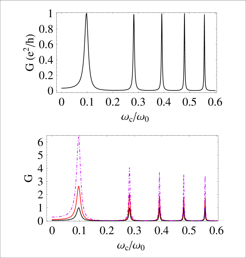
Figure 3: (Top) Ballistic conductance as a function of the magnetic field: the use of a double square barrier model, for the cavity formed by two QPCs, allows for the exploration of the backward scattering oscillations due to the magnetic field. We observe the appearing of resonance peaks, as a function of the magnetic field. (Bottom) Magnetic field dependent conductance obtained for $3$ different values of the temperature, following the CST theory (the solid line corresponds to the top panel with the lowest temperature $T_{0}$ while the dashed line corresponds to a higher value of $T\approx 1.2T_{0}$). The observed reduction of the peaks height corresponds to the predicted reduction of $\alpha_{end}$ with $B$.

It is quite interesting to analyze the correspondence between the resonance peaks in the conductance and the geometry of the current vector field (see Fig.(4)) for strong magnetic fields, starting from the usual resonance condition: the $n-th$ peak corresponds to $k_{F}d\approx n\pi$.

Some papers about the ballistic transport in the presence of a magnetic fieldvw discuss the presence of the conductance peaks, interpreting it as the evidence of an Aharonov-Bohm effect. We can explain that, by considering the localization of the edge states in the wire ($\langle x\rangle=\pm\gamma_{\omega}k_{F}$), so that the path of the electrons encloses a surface $S=2\gamma_{\omega}k_{F}d$. In the limit of strong $B$ ($\gamma_{\omega}\approx(\hbar)/(m_{e}\omega_{c})$), we obtain a value for the flux of $B$ in the presence of a transmission peak

$$\Phi_{S}(B)\approx B(2\gamma_{\omega}k_{F}d)\approx\frac{2c\hbar}{e}k_{F}d\approx n\frac{2ch}{e}=n\Phi_{0}.$$

Figure 4: The current vector field between the barriers, in the resonance and the off resonance conditions, for two square barriers, in the presence of a magnetic field.

This can also be seen by analyzing the presence of an integer number of ”circles of current”, between the two barriers, in correspondence to the peaks (see Fig.(4.left)). In Fig.(4.right) we show the off resonance behaviour corresponding to $|t|=0$. In both Figs. (4) each circle of current represents one electron which brings a quantum of magnetic flux $\Phi_{0}$.

Following the theoretical approach to the TLl in the presence of two barrierskf ; kf2 ; Furusaki ; Furusaki98 , we can calculate the resonant scattering condition, which can give rise to perfect transmission even for $K<1$. It corresponds to an average particle number between the two barriers of the form $\nu+1/2$, with integer $\nu$, i.e. the QD is in a degenerate state. If interactions between the electrons in the QD are included, one can recover the physics of the Coulomb blockadekf ; kf2 ; Furusaki ; Furusaki98 . The main difference is due to the temperature dependence of the conductance $G_{max}$. For the calculation of this dependence we can follow the CST mechanism recently proposedPostma01 , in order to explain the unconventional power-law dependencies in the measured transport properties of a CN. In this theory the electrons tunnel coherently, from the end of one CN lead to the end of the other CN lead, through a quantum state in the island. In this picture, the island should be regarded as a single impurity. The power law dependence of the conductance due to this tunneling mechanism is reported in eq.(7) and is shown in Fig.(3.bottom).

IV Conclusions

In this paper we showed how the presence of a magnetic field modifies the role played by both the e-e interaction and the presence of obstacles in a QW.

The first prediction that comes from our study is that the bulk critical exponent $\alpha_{bulk}$ of a semiconductor QW should be 10 times larger than the one measured in a typical CN according to the experimental results. We also predict a significant reduction of both critical exponents as the magnetic field is increased. The magnetic dependent value of $\alpha_{end}$ determines the temperature dependent $G$ in the sequential tunneling regime.

Our second prediction concerns the presence of some peaks in the small bias conductance versus magnetic field when two QPCs in are put series along a QW, forming an intrinsic QD (see Fig.(3)). The presence of magnetic field dependent peaks in the transmission can be used, in order to construct a ”magnetic field transistor” also in the temperature regime corresponding to the Luttinger liquid (a room temperature transistor, if we look at the device proposed in ref(Postma01 )). Thus we take into account a semiconducting QW made in $AsGaAs$ 2DEG, which typically have a length $L\sim 10-100\mu m$ and a width $20-30nm$, i.e. $\hbar\omega_{d}\approx 50-100meV$. The corresponding magnetic energy $\hbar\omega_{c}/B\approx 15meV/T$ is comparable with the confining one $\hbar\omega_{d}$, while the strong renormalization of the effective electron mass reduces by a factor $100$ the Zeeman spin splitting. If we fix two QPCs at a distance $d\approx 200-250nm$, we predict that some peaks (about $5-10$) have to be observed in the conductance, for values of the magnetic field between $0$ and $4$ T. The effects of very strong magnetic fields (much larger than those considered here) can dramatically change the behaviour of the system, as we showed in our previous papernoiqw , where we discussed also the spin polarization in QWs.

Our third result concerns the two different explanation for the peaks in the conductance. The discussed on-resonance condition in the TLl approach corresponds to the presence of an average particle number, $\nu$, in the cavity formed by the QPCs. On the contrary, the presence of a quantized circulating current, corresponding to the conductance peaks, was read as providing evidence of an Aharonov-Bohm effect in the ballistic regime. Thus we suggest that each electron in the QD has to bring a magnetic flux quantum.

References

- (1) A. De Martino and R. Egger, Europhys. Lett. 56, 570 (2001).
- (2) S. Tomonaga, Prog. Theor. Phys. 5, 544 (1950); J. M. Luttinger, J. Math. Phys. 4, 1154 (1963); D. C. Mattis and E. H. Lieb, J. Math. Phys. 6, 304 (1965).
- (3) For a review see J. Sólyom, Adv. Phys. 28, 201 (1979) and J. Voit, Rep. Prog. Phys. 57, 977 (1994).
- (4) C. L. Kane and M. P. A. Fisher, Phys. Rev. B 46, 15233 (1992)
- (5) A. H. MacDonald, Phys. Rev. Lett. 64, 220 (1990); X.-G. Wen, Phys. Rev. Lett. 64, 2206 (1990); Phys. Rev. B 41, 12838 (1990); Phys. Rev. B 43, 11025 (1991); Int. J. Mod. Phys. B 6, 1711 (1992); U. Zülicke and A. H. MacDonald, Phys. Rev. B 54, 16813 (1996).
- (6) A. Furusaki and N. Nagaosa, Phys. Rev. B 47, 4631 (1993).
- (7) S. J. Tans, M. H. Devoret, H. Dai, A. Thess, R. E. Smalley, L. J. Geerligs and C. Dekker, Nature 386, 474 (1997); M. Bockrath, D. H. Cobden, J. Lu, A. G. Rinzler, G. Andrew, R. E. Smalley, L. Balents and P. L. McEuen, Nature 397, 598 (1999); Z. Yao, H. W. J. Postma, L. Balents, and C. Dekker, Nature 402, 273 (1999).
- (8) R. Egger and A. O. Gogolin, Phys. Rev. Lett. 79, 5082 (1997); C. Kane, L. Balents and M. P. A. Fisher, ibid. 79, 5086 (1997).
- (9) S. Tarucha, T. Honda and T. Saku, Solid State Comm. 94, 413 (1995).
- (10) A. Yacoby, H. L. Stormer, N. S. Wingreen, L. N. Pfeiffer, K. W. Baldwin and K. W. West, Phys. Rev. Lett. 77, 4612 (1996); O. M. Auslaender, A. Yacoby, R. de Picciotto, K. W. Baldwin, L. N. Pfeiffer and K. W. West, Phys. Rev. Lett. 84, 1764 (2000); M. Rother, W. Wegscheider, R. A. Deutschmann, M. Bichler and G. Abstreiter, Physica E 6, 551 (2000).
- (11) S. Bellucci and J. González, Eur. Phys. J. B 18, 3 (2000); S. Bellucci, Path Integrals from peV to TeV, eds. R. Casalbuoni, et al. (World Scientific, Singapore, 1999) p.363, hep-th/9810181; S. Bellucci and J. González, Phys. Rev. B 64, 201106(R) (2001).
- (12) S. Bellucci, J. González and P. Onorato, Nucl. Phys. B 663 [FS], 605 (2003).
- (13) S. Bellucci, J. González and P. Onorato, Phys. Rev. B 69, 085404 (2004); S. Bellucci and P. Onorato, Phys. Rev. B 71 075418 (2005); S. Bellucci, J. González, P. Onorato, cond-mat/0501201.
- (14) H. J. Schulz, cond-mat/9503150.
- (15) H.W.Ch. Postma, T. Teepen, Z. Yao, M. Grifoni, and C. Dekker, Science 293, 76 (2001).
- (16) D. Bozovic, M. Bockrath, J.H. Hafner, C. M. Lieber, H. Park, and M. Tinkham, Appl. Phys. Lett. 78, 3693 (2001).
- (17) C. L. Kane and M. P. A. Fisher, Phys. Rev. Lett. 68, 1220 (1992); C. L. Kane and M. P. A. Fisher, Phys. Rev. B 46, 7268 (1992)
- (18) A. Furusaki and N. Nagaosa, Phys. Rev. B 47, 3827 (1993).
- (19) M. Sassetti, F. Napoli, and U. Weiss, Phys. Rev. B 52, 11213 (1995).
- (20) A. Furusaki, Phys. Rev. B 57, 7141 (1998).
- (21) A. Braggio, M. Grifoni, M. Sassetti, and F. Napoli, Europhys. Lett. 50, 236 (2000).
- (22) M. Thorwart, M. Grifoni, G. Cuniberti, H.W.Ch. Postma, and C. Dekker, Phys. Rev. Lett. 89, 196402 (2002).
- (23) Yu.V. Nazarov and L.I. Glazman, Phys. Rev. Lett. 91, 126804 (2003).
- (24) D.G. Polyakov and I.V. Gornyi, Phys. Rev. B 68, 035421 (2003).
- (25) A. Komnik and A.O. Gogolin, Phys. Rev. Lett. 90, 246403 (2003).
- (26) S. Hügle and R. Egger, Europhys. Lett. 66, 565 (2004).
- (27) C.W. J. Beenakker, Phys. Rev. B 44, 1646 (1991).
- (28) T. J. Thornton, Rep. Prog. Phys. 58, 311 (1995).
- (29) S. V. Zaitsev-Zotov ,Yu A. Kumzerov, Yu A. Firsov and P. Monceau J. Phys.: Condens. Matter 12, L303-L309 (2000).
- (30) S. Bellucci and P. Onorato, Eur. Phys. J. B - Condensed Matter 45, 87-96 (2005).
- (31) S. Bellucci and P. Onorato, submitted to Phys. Rev. B (2005).
- (32) A. Kanda, K. Tsukagoshi, Y. Aoyagi and Y. Ootuka, Phys. Rev. Lett. 92, 36801 (2004).
- (33) B. J. van Wees, L. P. Kouwenhoven, C. J. P. M. Harmans, J. G. Williamson, C. E. Timmering, M. E. I. Broekaart, C. T. Foxon and J. J. Harris, Phys. Rev. Lett. 62, 2523 (1989).
- (34) S. Bellucci and P. Onorato, Phys. Rev. B 68, 245322 (2003).
- (35) L. Balents, M.P.A. Fisher, Phys. Rev. B 55, R11973 (1997).
- (36) R. Egger, A.O. Gogolin, Phys. Rev. Lett. 79, 5082 (1997).
- (37) R. Egger and A.O. Gogolin, Eur. Phys. J. B 3, 281 (1998).