Analysis of a long-range random field quantum antiferromagnetic Ising model

Abstract

We introduce a solvable quantum antiferromagnetic model. The model, with Ising spins in a transverse field, has infinite range antiferromagnetic interactions and random fields on each site following an arbitrary distribution. As is well-known, frustration in the random field Ising model gives rise to a many valley structure in the spin-configuration space. In addition, the antiferromagnetism also induces a regular frustration even for the ground state. In this paper, we investigate analytically the critical phenomena in the model, having both randomness and frustration and we report some analytical results for it.

I Introduction

With the realization in the mid last century that the Néel state cannot be the ground state (not even an eigenstate) of a quantum Heisenberg antiferromagnet, considerable effort has gone in search of, and in understanding the nature of, the ground state of such and similar quantum antiferromagnet Frad . Since early 1960s, quantum spin systems described by Ising model in a transverse tunneling field was investigated extensively; particularly because of easy mapping of the quantum system to its equivalent classical system and some cases of exact solubility Bikas . However there have, so far, been very few soluble models with antiferromagnetic interactions. It is well-known that the Ising model with long range interactions is solved exactly, even if the system has some special kind of quenched disorder, like in Sherrington-Kirkpatrick model of spin glasses. The number of degenerate states there can be estimated to be ${\cal O}(2^{N/2})$, which is larger than that of the above mentioned model (${\cal O}(2^{0.28743N})$). However, it is not so easy to consider the antiferromagnetic version of the model due to a lack of sub-lattice to capture the Néel ordering at low temperatures. In this paper, we introduce and study a solvable quantum antiferromagnetic model. In our model system each spin is influenced by the infinite range antiferromagnetic interactions in a transverse field. We also consider the case under the Gaussian or the binary random fields. By introducing two sub-groups of the spin system, we describe the system by means of the effective single spin Hamiltonian which is derived by the Trotter decomposition Suzuki and Hubberd-Stratonovich transformation Chaikin , and we solve the model analytically. A preliminary study, for the case without random fields, was reported earlier Cond .

This paper is organized as follows. In the next section, we introduce our model system and write down the general formula of the averaged free energy density. In section 3, to check the validity of our analysis, we compare our result with the previous well-known result which was obtained by mean-field approximations Kittel . In section 4, we consider the system under the Gaussian and the binary random fields on site and derive the equations of states and evaluate them. We then obtain the phase diagrams. Section 5 gives a summary.

II The model system and its analysis

In order to capture the N$\acute{\rm e}$el ordering below the critical temperature $T_{N}$ or the amplitude of transverse field $\Gamma_{N}$, we divide spins $S$ into the sub group $A$ : $\mbox{\boldmath$S$}^{(A)}=(S_{1}^{x,z,(A)},S_{2}^{x,z,(A)},\cdots,S_{N}^{x,z,(A)})$ and the sub group $B$ : $\mbox{\boldmath$S$}^{(B)}=(S_{1}^{x,z,(B)},S_{2}^{x,z,(B)},\cdots,S_{N}^{x,z,(B)})$, which are corresponding to virtual sub-lattice $A$ and B. Then the system is described by the following effective Hamiltonian

$$H(\mbox{\boldmath$\tau$})=\frac{J}{N}\sum_{ij}S_{i}^{z,(A)}S_{j}^{z,(B)}-\sum_{l=A,B}\Gamma_{l}\sum_{i}S_{i}^{x,(l)}-h\sum_{l=A,B}\sum_{i}h_{i}S_{i}^{z,(l)},$$ (1)

where $S_{i}^{z,(A,B)},S_{i}^{x,(A,B)}$ are $x$ and $z$ components of the Pauli matrix :

$$S_{i}^{x,(A,B)}=\left(\begin{array}[]{cc}0&1\\ 1&0\end{array}\right),\,\,\,S_{i}^{z,(A,B)}=\left(\begin{array}[]{cc}1&0\\ 0&-1\end{array}\right),$$ (6)

and $\mbox{\boldmath$h$}=(h_{1},h_{2},\cdots,h_{N})$ is a vector of the random fields on site and $h$ means the strength of the random field. $\Gamma_{A}$ and $\Gamma_{B}$ are amplitudes of the transverse fields in the sub groups $A$ and B. The main advantage of this Hamiltonian is that it can be recast exactly to that of a single spin in an effective field.

Using the Suzuki-Trotter formalism Suzuki one can express the quenched-variable $h$-dependent partition function as

$$Z(\mbox{\boldmath$h$}) = \lim_{M\to\infty}{\rm tr}_{\mbox{\boldmath$S$}_{A},\mbox{\boldmath$S$}_{B}}{\rm e}^{-\beta H(\mbox{\boldmath$h$})},$$ (7)

with

$$\beta H(\mbox{\boldmath$h$}) = \frac{\beta J}{2NM}\sum_{k}\left\{\sum_{i}S_{ik}^{(A)}+\sum_{i}S_{ik}^{(B)}\right\}^{2}-\frac{\beta J}{2NM}\sum_{k}\left\{\sum_{i}S_{ik}^{(A)}-\sum_{i}S_{ik}^{(B)}\right\}^{2}$$ (8)

$$- \frac{\beta h}{M}\sum_{i,k}h_{i}S_{ik}^{(A)}-\frac{\beta h}{M}\sum_{i,k}h_{i}S_{ik}^{(B)}-\gamma_{A}\sum_{i,k}S_{ik}^{(A)}S_{ik+1}^{(A)}-\gamma_{B}\sum_{i,k}S_{ik}^{(B)}S_{ik+1}^{(B)},$$

where $\gamma_{A,B}=\frac{1}{2}\log\coth\left(\frac{\beta\Gamma_{A,B}}{M}\right).$ By using the Hubberd-Stratonovich transformation Chaikin , the field $h$-dependent partition function is written by means of the saddle point technique, in the limit $N\to\infty$, as

$$Z(\mbox{\boldmath$h$}) = {\rm tr}_{\mbox{\boldmath$S$}_{A},\mbox{\boldmath$S$}_{B}}\int_{-\infty}^{\infty}\int_{-i\infty}^{+i\infty}\prod_{k=1}^{M}\frac{idm_{+}^{k}dm_{-}^{k}}{(2\pi/N\beta J)}\,{\rm e}^{\frac{N\beta J}{2M}\sum_{k}(m_{+}^{k})^{2}-\frac{N\beta J}{2M}\sum_{k}(m_{-}^{k})^{2}}$$ (9)

$$\times {\exp}{\Biggr{[}}\frac{\beta J}{M}\sum_{i,k}m_{+}^{k}(S_{ik}^{(A)}+S_{ik}^{(B)})+\frac{\beta J}{M}\sum_{i,k}m_{-}(S_{ik}^{(A)}-S_{ik}^{(B)})$$

$$+ \frac{\beta h}{M}\sum_{i,k}\tau_{i}S_{ik}^{(A)}+\frac{\beta h}{M}\sum_{i,k}h_{i}S_{i,k}^{(B)}+\gamma_{A}\sum_{i,k}S_{ik}^{(A)}S_{ik+1}^{(A)}+\gamma_{B}\sum_{i,k}S_{ik}^{(B)}S_{ik+1}^{(B)}{\Biggr{]}}$$

$$\simeq {\rm e}^{\frac{N\beta J}{2M}\sum_{k}(m_{+}^{k})^{2}-\frac{N\beta J}{2M}(m_{-}^{k})^{2}}$$

$$\times {\rm tr}_{\mbox{\boldmath$S$}_{A},\mbox{\boldmath$S$}_{B}}{\exp}{\Biggr{[}}\frac{\beta J}{M}\sum_{i,k}m_{+}^{k}(S_{ik}^{(A)}+S_{ik}^{(B)})+\frac{\beta J}{M}\sum_{i,k}m_{-}^{k}(S_{ik}^{(A)}-S_{ik}^{(B)})$$

$$+ \frac{\beta h}{M}\sum_{i,k}h_{i}S_{ik}^{(A)}+\frac{\beta h}{M}\sum_{i,k}h_{i}S_{ik}^{(B)}+\gamma_{A}\sum_{i}S_{ik}^{(A)}S_{ik+1}^{(A)}+\gamma_{B}\sum_{i,k}S_{ik}^{(B)}S_{ik+1}^{(B)}{\Biggr{]}}$$

$$= {\rm e}^{\frac{N\beta J}{2M}\sum_{k}(m_{+}^{k})^{2}-\frac{N\beta J}{2M}(m_{-}^{k})^{2}}{\rm tr}_{\mbox{\boldmath$S$}_{A},\mbox{\boldmath$S$}_{B}}\prod_{i=1}^{N}{\exp}\left[-\beta H_{i}(h_{i})\right],$$

where $H_{i}(h_{i})$ is the effective single spin Hamiltonian and is given by

$$H_{i}(h_{i}) = -\frac{J}{M}\sum_{k}m_{+}^{k}(S_{ik}^{(A)}+S_{ik}^{(B)})-\frac{J}{M}\sum_{k}m_{-}^{k}(S_{ik}^{(A)}-S_{ik}^{(B)})$$ (10)

$$- \frac{hh_{i}}{M}\sum_{l=A,B}\sum_{k}S_{ik}^{(l)}-\beta^{-1}\sum_{l=A,B}\gamma_{l}S_{ik}^{(l)}S_{ik+1}^{(l)}.$$

Here we should keep in mind that the integrals with respect to $m_{+}^{k}$ and $m_{-}^{k}$ are evaluated at the saddle points in the limit of $N\to\infty$, namely

$$m_{+}^{k} = -\frac{1}{N}\sum_{i}S_{ik}^{(A)}+\frac{1}{N}\sum_{i}S_{ik}^{(B)}=-(M_{A}^{k,z}+M_{B}^{k,z})$$ (11)

$$m_{-}^{k} = \frac{1}{N}\sum_{i}S_{ik}^{(A)}-\frac{1}{N}\sum_{i}S_{ik}^{(B)}=(M_{A}^{k,z}-M_{B}^{k,z}),$$ (12)

where $m_{+}^{k}$ and $m_{-}^{k}$ are related to the magnetizations of $z$-component for group $A$ and $B$, namely $M_{A}^{k,z}$ and $M_{B}^{k,z}$. Thus the free energy $F(\mbox{\boldmath$h$})=-\beta^{-1}\log Z(\mbox{\boldmath$h$})$ of the system is now written by

$$F(\mbox{\boldmath$h$})=-\frac{NJ}{2M}\sum_{k}(m_{+}^{k})^{2}+\frac{NJ}{2M}\sum_{k}(m_{-}^{k})^{2}-\beta^{-1}\log\prod_{i=1}^{N}{\rm tr}_{S_{ik}^{(A)},S_{ik}^{(B)}}{\exp}\left[-\beta H_{i}(h_{i})\right].$$ (13)

Taking into account the symmetry of the system, $m_{+}^{k}=m_{+},m_{-}^{k}=m_{-}$ for all $k$, i.e., the so-called static approximation holds good naturally; the fluctuations due to, say, two-spin correlations (including entanglements) vanishes in thermodynamic limit. Thus the $h$-dependent free energy leads to

$$F(\mbox{\boldmath$h$})=-\frac{NJ}{2}(M_{A}^{z}+M_{B}^{z})^{2}+\frac{NJ}{2}(M_{A}^{z}-M_{B}^{z})^{2}-\beta^{-1}\log\prod_{i=1}^{N}{\cal Z}_{i}^{(A)}{\cal Z}_{i}^{(B)}$$ (14)

with

$${\cal Z}_{i}^{(A,B)}={\rm tr}_{S_{i}^{x,z,(A,B)}}{\rm e}^{\beta(-2JM_{B,A}^{z}+hh_{i})S_{i}^{z,(A,B)}+\beta\Gamma_{A,B}S_{i}^{x,(A,B)}},$$ (15)

where we used the relations (11) and (12): $m_{+}+m_{-}=-2M_{B}^{z},m_{+}-m_{-}=-2M_{A}^{z}$. It should be noted that the above free energy still depends on the fields $h$. To obtain the $h$-independent averaged free energy $F$, we should evaluate the following quantity

$$F = \int_{-\infty}^{\infty}P(\mbox{\boldmath$h$})F(\mbox{\boldmath$h$})d\mbox{\boldmath$h$},$$ (16)

where $P(\mbox{\boldmath$h$})=P(h_{1},\cdots,h_{N})$ is a joint distribution of the random fields and we defined $d\mbox{\boldmath$h$}=dh_{1}\cdots dh_{N}$. If we assume that the random field $h_{i}$ for each site $i$ is uncorrelated (not influenced by other $h_{j}{\rm{{}^{\prime}s}};~{}j\neq i$) then

$$P(\mbox{\boldmath$h$}) = P(h_{1},\cdots,h_{N})=P(h_{1})\cdots P(h_{N})=\prod_{i}P(h_{i}),$$ (17)

there in the average in (16), giving the free energy (per spin)

$$f=\sum_{l=A,B}f_{l},\,\,f_{l}=-JM_{l}^{z}M_{l+1}^{z}-\beta^{-1}\int_{-\infty}^{\infty}d\hat{h}P(\hat{h})\log 2\cosh\beta\sqrt{(2JM_{l}^{z}-h\hat{h})^{2}+\Gamma_{l+1}^{2}}.$$ (18)

Here we used the fact that the $2\times 2$ matrix $H$ (with the elements $(\mbox{\boldmath$H$})_{11}=-(\mbox{\boldmath$H$})_{22}=a,(\mbox{\boldmath$H$})_{12}=(\mbox{\boldmath$H$})_{21}=b$ appearing in the of exponent of equation (15)) has eigen values $\pm\sqrt{a^{2}+b^{2}}$. We also should keep in mind that in the sum with respect to $l$, $A+1=B,B+1=A$; hence $|A-B|=1$ is satisfied. Hereafter, we use this relation for the sum with respect to the label $l$. The magnetizations for two sub-lattices $M_{A}^{z}$ and $M_{B}^{z}$ now obey the following saddle point equations

$$M_{l}=\int_{-\infty}^{\infty}d\hat{h}P(\hat{h})\frac{-(2JM_{l+1}^{z}-h\hat{h})}{\sqrt{(2JM_{l+1}^{z}-h\hat{h})^{2}+\Gamma_{l}^{2}}}\tanh\beta\sqrt{(2JM_{l+1}^{z}-h\hat{h})^{2}+\Gamma_{l}^{2}},\,(l=A,B)$$ (19)

where it should be noted that $A-B=1$ and the appropriate expression for magnetization of each sub-lattice can be derived by equating $\partial f/\partial M_{B}^{z}$ and $\partial f/\partial M_{A}^{z}$ to zero respectively.

III Analysis under uniform field

We first consider the case of uniform field Cond , i.e., in (18) or (19), $\hat{h}\to 1$. In this limit, by using the fact $\int_{-\infty}^{\infty}d\hat{h}P(\hat{h})=1$, the free energy density $f$ reads

$$f=\sum_{l=A,B}f_{l}^{U};\,\,\,f_{l}^{U}=-JM_{l}^{z}M_{l+1}^{z}-\beta^{-1}\log 2\cosh\beta\sqrt{(2JM_{l}^{z}-h)^{2}+\Gamma_{l+1}^{2}}$$ (20)

and the saddle point equations with respect to $M_{A}^{z}$ and $M_{B}^{z}$ are obtained as follows.

$$M_{l}^{z}=\frac{(-2JM_{l+1}^{z}+h)}{\sqrt{(-2JM_{l+1}^{z}+h)^{2}+\Gamma_{l}^{2}}}\tanh\beta{\sqrt{(-2JM_{l+1}^{z}+h)^{2}+\Gamma_{l}^{2}}},\,\,\,(l=A,B).$$ (21)

Before we investigate the quantum effects, we check the classical case, that is $\Gamma_{A}=\Gamma_{B}=0$. Then, the above saddle point equations are reduced to

$$M_{l}^{z}=\tanh\beta(-2JM_{l+1}^{z}+h),\,\,\,\,(l=A,B).$$ (22)

In order to determine the N$\acute{\rm e}$el temperature, we expand the equations around $M_{A},M_{B}\simeq 0$ for $h=0$ and obtain $M_{A}^{z}\simeq-2J\beta M_{B}^{z},M_{B}^{z}\simeq-2J\beta M_{A}^{z}$. From these linearized equations, we find that only possible solution for the case of $M_{A}^{z}=M_{B}^{z}=M^{z}$ is $M^{z}=0$; whereas with N$\acute{\rm e}$el ordering a finite value of $M^{z}$ can be obtain: $M_{A}^{z}=-M_{B}^{z}=-M^{z}$. This gives the N$\acute{\rm e}$el temperature $T_{N}=\beta_{N}^{-1}=2J$. The linear susceptibilities $\chi_{A}$ and $\chi_{B}$ are then evaluated as

$$\chi_{l}=\lim_{h\to\infty}\frac{\partial M_{l}^{z}}{\partial h}=\frac{\beta(1-2J\chi_{l+1})}{\cosh^{2}\beta(-2JM_{l+1}^{z})},\,\,\,(l=A,B).$$ (23)

The behavior beyond the N$\acute{\rm e}$el temperature $T>T_{N}$ is determined by the condition $M_{A}^{z}\simeq 0,M_{B}^{z}\simeq 0$, i.e., $\chi_{A}=\beta(1-2J\chi_{B})$ and $\chi_{B}=\beta(1-2J\chi_{A})$. This leads to

$$\chi = \frac{2}{T+T_{N}}$$ (24)

where we defined $\chi=\chi_{A}+\chi_{B}$. Therefore, in the limit of $T\to T_{N}=J$, the linear susceptibility $\chi$ converges to $\chi\to 1/2J$. On the other hand, below the N$\acute{\rm e}$el temperature $T<T_{N}$, we find the solution for the N$\acute{\rm e}$el ordering : $M_{A}^{z}=-M_{B}^{z}=-M^{z}\neq 0$ for $h=0$. This condition should be satisfied for (cf. Eqn. (31))

$$\chi = \frac{2\beta}{2\beta J+\cosh^{2}\beta(2JM^{z})}$$ (25)

and at the critical point $T=T_{N},M=0$, the susceptibility takes $\chi=2/(2J+T_{N})=1/2J$. In Fig. 1 (left) we plot the shape of the susceptibility $\chi$ as a function of $T$.

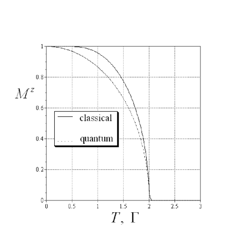
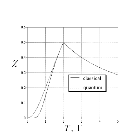
Figure 1: The longitudinal magnetization $M^{z}$ as a function of $T$ and $\Gamma$ for uniform systems (the left panel). The critical points of the second order phase transition are given by $T_{N}=\Gamma_{N}=1/2J$. The right panel shows the corresponding susceptibility $\chi$ as a function of $T$ and $\Gamma$.

From this figure we find that the susceptibility has a cusp, instead of the divergence as observed in the ferromagnetic systems, at the critical temperature $T=T_{N}$, as observed in the analysis for finite range models by using mean-field approximations Kittel . As mentioned earlier, this model being recastable exactly to a (classical) single-spin in an effective field (i.e., the mean-field approximation for the partition function being exact), there is no scope of any non-trivial wave-function with entangled neighbouring spins.

We next consider the quantum case $\Gamma_{A},\Gamma_{B}\neq 0$. For simplicity, we consider the case of the symmetric transverse field, namely, $\Gamma_{A}=\Gamma_{B}=\Gamma$. In order to consider the pure quantum effects, we take the limit of $\beta\to\infty$ and deal with the following coupled equations

$$M_{l}^{z}=\frac{-2JM_{l+1}^{z}+h}{\sqrt{(-2JM_{l+1}^{z}+h)^{2}+\Gamma^{2}}},\,\,\,(l=A,B).$$ (26)

It is important for us to bear in mind that for $J>0$, the above equations have a solution $M^{z}=0$ if $M_{A}=M_{B}$ and a solution $M^{z}\neq 0$ if $M_{A}=-M_{B},$ as expected. To determine the critical transverse field, we expand the above equations around $M_{A}^{z},M_{B}^{z}\simeq 0$ for $h=0$ as $M_{A}^{z}\simeq-2JM_{B}^{z}/\Gamma$ and $M_{B}^{z}\simeq-2JM_{A}^{z}/\Gamma$. This gives the critical point $\Gamma_{N}=2J$. The spontaneous sub-lattice order $M^{z}_{A}$ or $M^{z}_{B}$ vanishes at the Néel phase boundary $T_{N}(\Gamma)$. Deep inside the antiferromagnetic phase (at $\beta\rightarrow\infty,\Gamma\rightarrow 0,h=0$), $M_{A}^{z}=1=-M^{z}_{B}$ and the free energy density $f$ can be expressed as $f={1}/{\beta}\log[1+\exp(-\beta\Delta(\Gamma))]$, the specific heat $\partial^{2}f/\partial T^{2}$ will have a variation like $\exp[-\beta\Delta(\Gamma)]$ like that of a two level system with a gap $\Delta(\Gamma)={\sqrt{4J^{2}+\Gamma^{2}}}$ here. This is the exact magnitude of the gap in the magnon spectrum of this long range transverse Ising antiferromagnet.

The susceptibilities are given by

$$\chi_{l}=\lim_{h\to 0}\frac{\partial M_{l}^{z}}{\partial h}=\frac{\Gamma^{2}(1-2J\chi_{l+1})}{[(2JM_{l+1}^{z})^{2}+\Gamma^{2}]^{3/2}},\,\,\,\,(l=A,B)$$ (27)

Then, the behavior beyond the critical amplitude of the transverse field $\Gamma_{N}$ is determined by the condition $M_{A}^{z},M_{B}^{z}\simeq 0$, namely, $\chi_{A}=(1-2J\chi_{B})/\Gamma,\chi_{B}=(1-2J\chi_{A})/\Gamma$. This leads to

$$\chi = \chi_{A}+\chi_{B}=\frac{2}{\Gamma+\Gamma_{N}}.$$ (28)

On the other hand, below the critical amplitude of the transverse field $\Gamma_{N}$, we set $M_{A}^{z}=M_{B}^{z}=-M^{z}$ and obtain

$$\chi = \frac{2\Gamma^{2}}{[(2JM)^{2}+\Gamma^{2}]^{3/2}+2J\Gamma^{2}}.$$ (29)

At the critical point $\Gamma_{N}$ ($M^{z}=0$), the susceptibility is given as $\chi=2/(\Gamma_{N}+2J)=1/2J$. Around $\Gamma\simeq 0$, the susceptibility behaves as $\chi=2\Gamma^{2}/(2J)^{3}$. In Fig. 1 (right), we plot $\chi$ as a function of $\Gamma$ (and also $T$). From this figure, we find that the susceptibility has a cusp at the critical amplitude of the tunneling field.

We next investigate the transverse component of the susceptibility. The magnetization of the transverse direction are calculated the derivative of the free energy density with respect to the amplitudes of the transverse field $\Gamma_{A},\Gamma_{B}$.

$$M_{l}^{x}=\frac{\partial f}{\partial\Gamma_{l}}=\frac{\Gamma_{l}}{\sqrt{(-2JM_{l+1}^{z}+h)^{2}+\Gamma_{l}^{2}}}\tanh\beta\sqrt{(2JM_{l+1}^{z}+h)^{2}+\Gamma_{l}^{2}},\,\,\,(l=A,B)$$ (30)

At the ground state, these coupled equations are simplified as follows.

$$M_{l}^{x}=\frac{\Gamma_{l}}{\sqrt{(-2JM_{l+1}^{z}+h)^{2}+\Gamma_{l}^{2}}},\,\,\,(l=A,B)$$ (31)

In para-magnetic phase is specified by $M_{A}^{z}=M_{B}^{z}=0$ and this gives $M_{A}^{x}=M_{B}^{x}=1$. On the other hand, antiferromagnetic phase for $h=0$, we obtain from (26) as $M_{A}^{z}=-JM_{B}^{z}/\sqrt{(2JM_{B}^{z})^{2}+\Gamma_{A}^{2}},M_{B}^{z}=-JM_{A}^{z}/\sqrt{(2JM_{A}^{z})^{2}+\Gamma_{B}^{2}}$. Hence,

$$M_{l}^{x}=\frac{\Gamma_{l}}{2J},\,\,\,(l=A,B)$$ (32)

for the antiferromagnetic case $M_{A}^{z}=-M_{B}^{z}=-M$. Therefore, the susceptibilities of the transverse direction lead to

$$\chi^{\perp}=\chi_{l}^{x}=\frac{\partial M_{l}^{x}}{\partial\Gamma_{l}}=0,\,\,\,(l=A,B)$$ (33)

for $\Gamma_{A},\Gamma_{B}>\Gamma_{N}$ and

$$\chi^{\perp}=\chi_{A}^{x}=\chi_{B}^{x}=\frac{1}{J}$$ (34)

for $\Gamma_{A},\Gamma_{B}<\Gamma_{N}$. We plot the transverse magnetization $M^{x}=M_{A}^{x}=M_{B}^{x}$ for $M^{z}=M_{A}^{z}=M_{B}^{z}$ in Fig. 2.

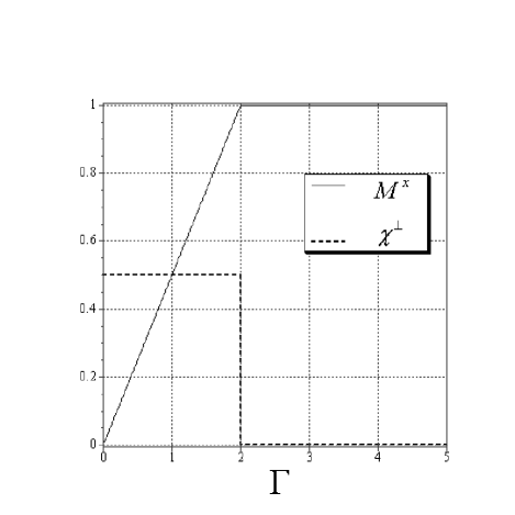
Figure 2: Longitudinal magnetization $M^{x}$ and susceptibility $\chi^{\perp}$.

We next consider the quantum antiferromagnetic system under random fields.

IV Analysis under random fields

In the previous section, we investigated the critical phenomena for spatially uniform systems. It has been conjectured that fluctuation in the random (longitudinal) field Ising model (RFIM) gives rise to a many valley structure in the configuration space, similar to the case in spin glasses. The study of the longitudinal random field transverse field Ising model with ferromagnetic uniform interactions has already been made Dutta . There seems to be no reported analytic research for the RFIM with antiferromagnetic interactions in transverse field. It should be interesting to investigate the competition between two different kinds of frustration; frustration due to the quenched disorder and the frustration induced by the antiferromagnetic interactions. In this section, we investigate quantum systems under random on-site longitudinal fields. In this paper, we consider the following two cases of the random field distributions :

$$P_{g}(\mbox{\boldmath$h$}) = \prod_{i=1}^{N}\frac{1}{\sqrt{2\pi}\sigma}{\exp}\left[-\frac{1}{2\sigma^{2}}(h_{i}-h_{0})^{2}\right]\equiv\prod_{i=1}^{N}P_{g}(h_{i})$$ (35)

$$\rm{and}\quad P_{b}(\mbox{\boldmath$h$}) = \prod_{i=1}^{N}\left\{\theta\delta(h_{i}-h_{0})+(1-\theta)\delta(h_{i}+h_{0})\right\}\equiv\prod_{i=1}^{N}P_{b}(h_{i}),$$ (36)

where the bias factor of the binary random field $\theta$ takes $0<\theta<1$. For these distributions, the free energy densities $f_{g,b}\equiv(1/N)\int_{-\infty}^{\infty}d\hat{h}P_{g,b}(\hat{h})F(\hat{h})$ become

$$f_{g} = \sum_{l=A,B}f_{l}^{g}$$ (37)

$$f_{l}^{g} = -JM_{l+1}^{z}M_{l}^{z}-\beta^{-1}\int_{-\infty}^{\infty}Dx\log 2\cosh\beta\sqrt{\{-2JM_{l+1}^{z}+h(\sigma x+h_{0})\}^{2}+\Gamma_{l}^{2}},$$ (38)

for the Gaussian random field $P_{g}(\mbox{\boldmath$h$})$, where $Dx\equiv\frac{1}{\sqrt{2\pi}}e^{{-x^{2}/2}}dx$ and

$$f_{b} = \sum_{l=A,B}f_{l}^{b}$$ (39)

$$f_{l}^{b} = -JM_{l+1}^{z}M_{l}^{z}-\beta^{-1}\theta\log 2\cosh\beta\sqrt{\{-2M_{l+1}^{z}J+hh_{0}\}^{2}+\Gamma_{l}^{2}}$$ (40)

$$- \beta^{-1}(1-\theta)\log 2\cosh\beta\sqrt{\{2M_{l+1}^{z}J+hh_{0}\}^{2}+\Gamma_{l}^{2}},$$

for the binary random field $P_{b}(\mbox{\boldmath$h$})$. In following, we investigate the critical phenomena given by these free energy densities for these two cases.

IV.1 The Gaussian random field

For the Gaussian random field (35) the saddle point equations are given by the derivative of the free energy density $f_{G}$ with respect to $M_{A}^{z}$ and $M_{B}^{z}$. Then we have

$$M_{l}^{z}=\int_{-\infty}^{\infty}Dx\frac{\{-2JM_{l+1}^{z}+h(\sigma x+h_{0})\}}{\sqrt{\{-2JM_{l+1}^{z}+h(\sigma x+h_{0})\}^{2}+\Gamma_{l}^{2}}}\tanh\beta\sqrt{\{-2JM_{l+1}^{z}+h(\sigma x+h_{0})\}^{2}+\Gamma_{l}^{2}}$$ (41)

for $l=A,B$. At the ground state $(\beta\to\infty)$ these equations of states are simplified as follows

$$M_{l}^{z}=\int_{-\infty}^{\infty}Dx\frac{\{-2JM_{l+1}^{z}+h(\sigma x+h_{0})\}}{\sqrt{\{-2JM_{l+1}^{z}+h(\sigma x+h_{0})\}^{2}+\Gamma_{l}^{2}}},\,\,\,(l=A,B).$$ (42)

For the possible choice $M_{A}^{z}=M^{z}=-M_{B}^{z}$ to detect the N$\acute{\rm e}$el ordering, we solve the above equations for the symmetric transverse fields $\Gamma_{A}=\Gamma_{B}=\Gamma$ numerically. In Fig. 3 (left), we plot the case of the center of the Gaussian, $h_{0}$ takes $h_{0}=0$ and the deviation of the Gaussian $\sigma=0.5$ and $1.5$. From this figure, we find that the system undergoes second-order phase transition at the critical amplitude of the transverse field from the behavior of $M^{z}$. If the phase transition is first order for the case of the center $h_{0}$ of the Gaussian (35) is zero, we can expand the saddle point equation with respect to $M_{A}^{z}$ under the condition $\Gamma_{A}=\Gamma_{B}=\Gamma$ and $M_{B}^{z}=-M_{A}^{z}=-M^{z}$ as

$$M^{z} = C_{1}M^{z}-C_{3}(M^{z})^{3}+{\cal O}((M^{z})^{5})$$ (43)

with

$$C_{1}=2J\Gamma^{2}\int_{-\infty}^{\infty}\frac{Dx}{[(h\sigma x)^{2}+\Gamma^{2}]^{3/2}},\,\,\,\,\,C_{3}=4J^{3}\Gamma^{2}\int_{-\infty}^{\infty}Dx\,\frac{2(h\sigma x)^{2}+\Gamma^{2}}{[(h\sigma x)^{2}+\Gamma^{2}]^{7/2}}.$$ (44)

The phase boundary $\Gamma(\sigma)$ of the continuous transition between the N$\acute{\rm e}$el and the paramagnetic phases is obtained for a given set of the parameters $(J,h_{0},h)$ by the condition $a=1$, namely

$$\Gamma=\left(2J\int_{-\infty}^{\infty}\frac{Dx}{[(h\sigma x)^{2}+\Gamma^{2}]^{3/2}}\right)^{-1/2}.$$ (45)

The second order phase transition is observed for $C_{3}>0$, whereas a first order phase transition is found for $C_{3}<0$. In Fig. 3 (right), we plot the boundaries between the N$\acute{\rm e}$el and the paramagnetic phases for both quantum and classical systems. In this plot, we set $(J,h,h_{0})=(1,1,0)$. In the left panel of Fig. 4, we plot the factor $C_{3}$ of the third order of the expansion of the magnetization $M^{z}$ as a function of $\sigma$. In this plot we substituted the solution of the boundary (45) for a given $\sigma$ into $C_{3}$. From this panel we find, that from the value $C_{3}=4(J/\Gamma)^{3}>0$ at $\sigma=0$, that $C_{3}$ decreases and takes its positive minima at just below the critical point $\sigma_{c}$, and beyond the critical point $C_{3}$ increases again. We therefore conclude that the phase transition is always second order.

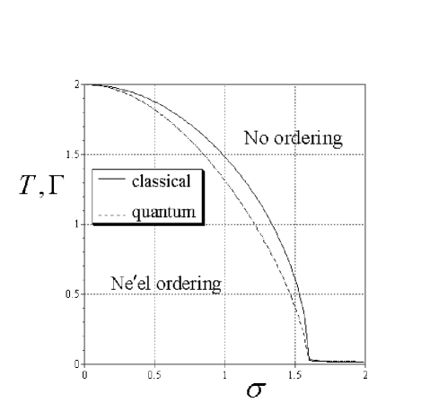
Figure 3: The right panel shows phase boundaries between antiferromagnetic and paramagnetic phases for classical and quantum systems for $(J,h,h_{0})=(1,1,1)$. The left panel shows the variation of longitudinal and transverse magnetizations $M^{z}$ and $M^{x}$ with $\Gamma$.

We might see this from the argument below. In the limit of $\Gamma\to 0$, the equation of state (42) for $M^{B}=-M_{A}^{z}=-M^{z}$ is simplified to

$$M^{z} = \int_{-\infty}^{\infty}Dx\,{\rm sgn}\left(2JM^{z}+h\sigma x\right)=1-2H\left(\frac{2JM^{z}}{h\sigma}\right).$$ (46)

In Fig. 4 (right panel), we plot the solution of (46) for several values of $h$.

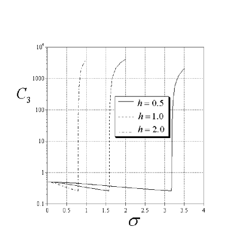
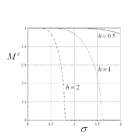
Figure 4: The longitudinal magnetization $M^{z}$ as a function of $\sigma$ for several values of $h_{0}$ for the case of $\Gamma=0$ (right panel). Each line of a solution of the equation (46). The left panel shows the $\sigma$-dependence of the factor $C_{3}$ of the third order of the magnetization near the critical point.

We found that for $\sigma\to\infty$, $H(2JM^{z}/h\sigma)\to 1/2$ and $M^{z}\to 0$, whereas, for $\sigma\to 0$, $H(2JM^{z}/h\sigma)\to 0$ and $M^{z}\to 1$. By expanding (46) with respect to $M^{z}$ up to the first order, we obtain the critical point $\sigma_{c}$ as

$$\sigma_{c}=\sqrt{\frac{2}{\pi}}\left(\frac{2J}{h}\right).$$ (47)

The magnetization varies continuously near this critical point (of the second order phase transition): $M^{z}=\sqrt{12\sigma/\pi\sigma_{c}}(1-\sigma/\sigma_{c})^{1/2}$.

We next evaluate the $x$-component (the transverse component) of the magnetizations $M_{A}^{x}$ and $M_{B}^{x}$. These are calculated at the ground state $\beta\to\infty$ as

$$M_{l}^{x}=\frac{\partial f_{G}}{\partial\Gamma_{l}}=\int_{-\infty}^{\infty}\frac{\Gamma_{l}Dx}{\sqrt{\{-2JM_{l+1}^{z}+h(\sigma x+h_{0})\}^{2}+\Gamma_{l}^{2}}},\,\,\,(l=A,B)$$ (48)

In Fig. 3 (left panel), we plot the results. It should be noted that in the limit of $\Gamma\to\infty$, $M^{x}$ saturates $M^{x}\simeq\int_{-\infty}^{\infty}Dx(\Gamma/\Gamma)=1$.

IV.2 The binary random fields

For the binary random fields, we obtain the saddle point equations by taking the derivative of the free energy density $f_{B}$ with respect to $M_{A}^{z}$ and $M_{B}^{z}$ as follows:

$$M_{l}^{z} = -\frac{\theta(2JM_{l+1}^{z}-hh_{0})}{\sqrt{(2JM_{l+1}^{z}-hh_{0})^{2}+\Gamma_{l}^{2}}}\tanh\beta\sqrt{(2JM_{l+1}^{z}-hh_{0})^{2}+\Gamma_{l}^{2}}$$ (49)

$$- \frac{(1-\theta)(2JM_{l+1}^{z}+hh_{0})}{\sqrt{(2JM_{l+1}^{z}+hh_{0})^{2}+\Gamma_{l}^{2}}}\tanh\beta\sqrt{(2JM_{l+1}^{z}+hh_{0})^{2}+\Gamma_{l}^{2}},\,\,\,(l=A,B).$$

At the ground state $\beta\to\infty$, these equations are simplified to

$$M_{l}^{z}=-\frac{\theta(2JM_{l+1}^{z}-hh_{0})}{\sqrt{(2JM_{l+1}^{z}-hh_{0})^{2}+\Gamma_{l}^{2}}}-\frac{(1-\theta)(2JM_{l+1}^{z}+hh_{0})}{\sqrt{(2JM_{l+1}^{z}+hh_{0})^{2}+\Gamma_{l}^{2}}},\,\,\,(l=A,B).$$ (50)

We solve the above equations numerically and plot it in Fig. 5 (left panel). From this figure, we find that the system undergoes first order phase transition when the value of $h_{0}$ is larger than same critical point $h_{0}^{c}$. Whereas, for small value of $h_{0}<h_{0}^{c}$, the phase transition is the second order.

In following, we determine the tri-critical point $(h_{0}^{c},\Gamma_{c})$. If the transition is continuous, we can expand the saddle point equation for $M_{A}^{z}$ under the condition $\Gamma_{A}=\Gamma_{B}=\Gamma$ and $M_{B}^{z}=-M_{A}^{z}=-M^{z}$ as follows:

$$M^{z} = \tilde{C}_{0}+\tilde{C}_{1}M^{z}+\tilde{C}_{2}(M^{z})^{2}+\tilde{C}_{3}(M^{z})^{3}+{\cal O}((M^{z})^{4})$$ (51)

where we defined

$$\tilde{C}_{0} = \frac{2(\theta-1)hh_{0}}{\sqrt{(hh_{0})^{2}+\Gamma^{2}}}$$ (52)

$$\tilde{C}_{1} = \frac{2J\Gamma^{2}}{\{(hh_{0})^{2}+\Gamma^{2}\}^{3/2}}$$ (53)

$$\tilde{C}_{2} = -2J^{2}hh_{0}(2\theta-1)\left[\frac{\Gamma^{2}+4(hh_{0})^{2}}{\{(hh_{0})^{2}+\Gamma^{2}\}^{5/2}}\right]$$ (54)

$$\tilde{C}_{3} = 4J^{3}\left[\frac{\Gamma^{4}-4\Gamma^{2}(hh_{0})^{2}}{\{(hh_{0})^{2}+\Gamma^{2}\}^{7/2}}\right].$$ (55)

Therefore, if the distribution (36) is symmetric (i.e., $\theta=1/2$), the factors $\tilde{C}_{0}$ and $\tilde{C}_{2}$ vanish and the magnetization behaves as

$$M^{z} = \tilde{C}_{1}M^{z}+\tilde{C}_{3}(M^{z})^{3}+{\cal O}((M^{z})^{5}).$$ (56)

From this expression, we find that a second order phase transition is found when the condition $\tilde{C}_{1}=1$ and $\tilde{C}_{3}<0$ holds. On the other hand, a first order phase transition is observed for $\tilde{C}_{1}=1$ and $\tilde{C}_{3}>0$. Therefore, the point $(h_{0}^{c},\Gamma_{c})=((J/h)(4/5)^{3/2},2J(4/5)^{3/2})$, which is determine by $\tilde{C}_{1}=1,\tilde{C}_{3}=0,$ corresponds to a tri-critical point on the phase boundary. In Fig. 5 (right panel) we plot these phase boundaries. We should notice that the critical point $\Gamma_{c}$ is independent of $h$. We find that for $h_{0}>h_{0}^{c}$, the transition from the symmetry breaking phase to symmetric phase is first order. To compare this result with the case of the Gaussian random field, we consider the limit $\Gamma\to 0$ in (50). We obtain

$$M_{l}^{z}=\theta\,{\rm sgn}(2JM_{l+1}^{z}+hh_{0})+(1-\theta)\,{\rm sgn}(2JM_{l+1}^{z}-hh_{0}),\qquad(l=A,B).$$ (57)

To detect the transition point between the N$\acute{\rm e}$el and paramagnetic phases, we set $M_{l}^{z}=M^{z}=-M_{l+1}^{z}$ and $\theta=1/2$ for simplicity. We then have

$$2M^{z}={\rm sgn}(2JM^{z}+hh_{0})+{\rm sgn}(2JM^{z}-hh_{0}).$$ (58)

Apparently, $M_{z}$ takes values $1$ or $0$ and the critical point of the first order phase transition is determined by $2J-hh_{0}=0$, i.e., $h_{0}^{c}=2J/h$. This point $h_{0}^{c}$ is observed on the crossing point on the $h_{0}$-axis in Fig. 5 (right panel). On the other hand, as we saw in Fig. 4 (left panel), the magnetization $M^{z}$ for the Gaussian random field drops gradually and the phase transition is second order even if there is no quantum fluctuation $\Gamma=0$ at the ground state (at $\beta\to\infty$). This is a reason why the order-disorder phase transition in the Gaussian random field Ising model is always first order and it does not depend on $\Gamma$ or $\sigma$.

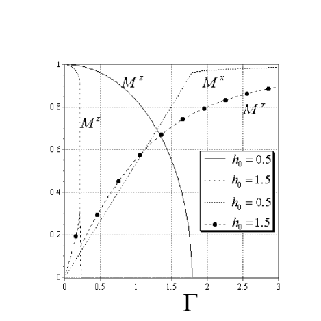
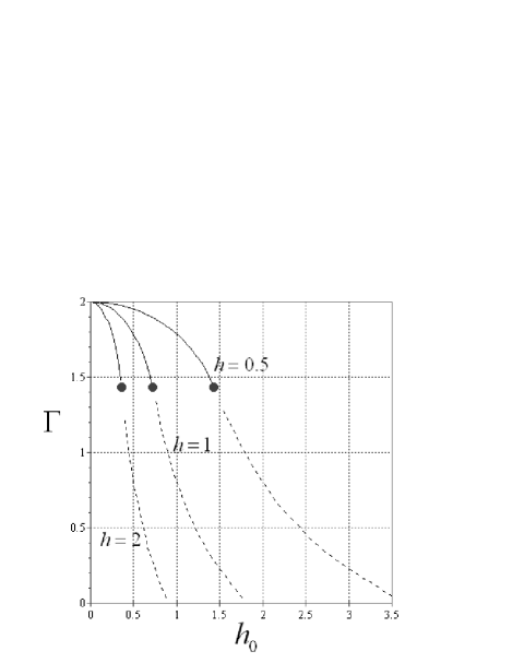
Figure 5: The longitudinal and the transverse magnetizations, $M^{z}$ and $M^{x}$ as a function of $\Gamma$ for the case of the binary random fields (right panel). The left panel shows phase boundaries between antiferromagnetic and paramagnetic phases. The dots represent tri-critical points $(h_{0}^{c},\Gamma_{c})=((1/h)(4/5)^{3/2},2(4/5)^{3/2})$ we set $J=1$.

Finally, we calculate the transverse magnetization $M_{A}^{x}$ and $M_{B}^{x}$. From the derivative of the free energy density $f_{B}$ with respect to $\Gamma_{A}$ and $\Gamma_{B}$, we obtain

$$M_{l}^{x} = \frac{\partial f_{b}}{\partial\Gamma_{l}}=\frac{\theta\Gamma_{l}}{\sqrt{\{-2JM_{l+1}^{z}+hh_{0}\}^{2}+\Gamma_{l+1}^{2}}}\tanh\beta\sqrt{\{-2JM_{l+1}^{z}+hh_{0}\}^{2}+\Gamma_{l}^{2}}$$ (59)

$$+ \frac{(1-\theta)\Gamma_{l}}{\sqrt{\{2JM_{l+1}^{z}+hh_{0}\}^{2}+\Gamma_{l}^{2}}}\tanh\beta\sqrt{\{2JM_{l+1}^{z}+hh_{0}\}^{2}+\Gamma_{l}^{2}},\,\,\,(l=A,B).$$

At the ground state, these equations are simplified as

$$M_{l}^{x}=\frac{\theta\Gamma_{l}}{\sqrt{\{-2JM_{l+1}^{z}+hh_{0}\}^{2}+\Gamma_{l}^{2}}}+\frac{(1-\theta)\Gamma_{l}}{\sqrt{\{2JM_{l+1}^{z}+hh_{0}\}^{2}+\Gamma_{l}^{2}}},\,\,\,(l=A,B).$$ (60)

In Fig. 5 (left panel) we plot the transverse magnetization for case of the symmetric amplitude of the tunneling field $\Gamma_{A}=\Gamma_{B}=\Gamma$ as a function of $\Gamma$. Obviously, for large $\Gamma$, we found $M^{x}=1$ from (60).

As may be noted, in the case where the random quenched fields are symmetrically distributed about its zero value, the effective sub-lattice symmetry could be utilized to reduce the whole problem to that of a ferromagnet.

V Summary

In this paper, we proposed an analytically solvable quantum antiferromagnetic Ising model. Because of Ising anisotropy and long-range interactions, it has solvable Néel-like ground and other state properties. In view of the extensive recent studies in quantum antiferromagnets (Kaiser -Moessner2 ), particularly in quantum Ising antiferromagnets (Moessner ,Moessner2 ), this kind of analysis should be of considerable importance.

In the analysis of spatially uniform system, we found the Néel order below the tunneling field $\Gamma_{N}$ and show that the linear susceptibility has a cusp variation around that critical $\Gamma_{N}$. It may be mentioned that a similar behavior in the half-filled Hubberd model was observed earlier Stefan .

For this uniform spin system, the free energy density (20) gives the ground state energy in the zero temperature limit and it also gives the low temperature behavior of the specific heat, the exponential variation of which gives the precise gap magnitude $\Delta(={\sqrt{4J^{2}+\Gamma^{2}}})$ in the excitation spectrum of the system. It may be noted that, because of the restricted (Ising) symmetry and the infinite dimensionality (long range interaction) involved, there need not be any conflict with the Haldane conjecture. Although our entire analysis has been for spin-1/2 (Ising) case, because of the reduction of the effective Hamiltonian (10) to that of a single spin in an effective vector field, the results can be easily generalized for higher values of the spin $S$. No qualitative change is observed. The order-disorder transition in the model can be driven both by thermal fluctuations (increasing $T$) or by the quantum fluctuations (increasing $\Gamma$). This transition in the model has been investigated studying the behaviors of the (random sub-lattice) staggered magnetization and the (longitudinal and transverse) susceptibilities. No quantum phase transition, where the gap $\Delta$ vanishes, is observed in the model, unlike in the one dimensional transverse Ising antiferromagnets.

By analysis of the disordered system as the random field Ising model in a transverse field, we found that the order of the phase transition changes at a tri-critical point. These conditions are obtained analytically for both the Gaussian random fields and the binary random fields. We believe, analysis of such model systems might provide some insights also for the quantum antiferromagnets with short range interactions.

- (1) See e.g., E. Fradkin, Field Theories of Condensed Matter Systems, Addison-Wesley, Redwood (1991); I. Bose in Frontiers in Condensed Matter Physics: 75th year special publication of Ind. J. Phys., Eds. J. K. Bhattacharjee and B. K. Chakrabarti, Allied Publ., New Delhi (2005).
- (2) B. K. Chakrabarti, A. Dutta and P. Sen, Quantum Ising Phases and Transitions in Transverse Ising Models, Springer, Heidelberg (1996).
- (3) M. Suzuki, Prog. Theor. Phys. 56, 2454 (1976); see also B. K. Chakrabarti and A. Das, pp 3-36 and N. Hatano and M. Suzuki, pp 37-68 in Quantum Annealing and Related Optimization Methods, Eds. A. Das and B. K. Chakrabarti, LNP 679, Springer, Heidelberg (2005)
- (4) See, e.g., P. M. Chaikin and T. C. Lubensky, Principles of Condensed Matter Physics, Cambridge University Press, Cambridge (1997).
- (5) B. K. Chakrabarti and J. Inoue, cond-mat/0508218 (2005); Proc. CMDAYS-05, Ind. J. Phys. (to be published).
- (6) See e.g., C. Kittel, Introduction to Solid State Physics, John Wiley Sons Inc., N.Y. (1966).
- (7) D. Sherrington and S. Kirkpatrick, Phys. Rev. Lett. 35, 1792 (1975).
- (8) T. Schneider and E. Pytte, Phys. Rev. B 15, 1519 (1976).
- (9) A. Dutta, B. K. Chakrabarti and R. B. Stinchcombe, J. Phys. A : Math. Gen. 29, 5285 (1996).
- (10) C. Kaiser and I. Peschel, J. Phys. A : Math. Gen. 22 4257 (1989).
- (11) T. Roscilde, P. Verrucchi, A. Fubini, S. Haas and V. Tognetti, Phys. Rev. Lett. 94, 147208 (2005).
- (12) R. Moessner, S. L. Sondhi and P. Chandra, Phys. Rev. Lett. 84, 4457 (2000).
- (13) R. Moessner and S. L. Sondhi, Phys. Rev. B 63, 224401 (2001).
- (14) G. Stefanucci and M. Cini, Phys. Rev. B 66, 115108 (2002).