Molecular motor traffic in a half-open tube

Abstract

The traffic of molecular motors which interact through mutual exclusion is studied theoretically for half-open tube-like compartments. These half-open tubes mimic the shapes of axons. The mutual exclusion leads to traffic jams or density plateaus on the filaments. A phase transition is obtained when the motor velocity changes sign. We identify the relevant length scales and characterize the jamming behavior using both analytical approximations and Monte Carlo simulations of lattice models.

1 Introduction

Biological cells exhibit complex patterns of intracellular traffic: vesicles shuttle between different cellular compartments, others travel from the cell center to the periphery or vice versa, but also filaments, RNA, chromosomes, and even viruses are permanently on the move within cells [1, 2]. An extreme example is the long-ranged transport of vesicles, organelles, and proteins along the axons of nerve cells [3], which can be up to a meter long. All this traffic is based on the molecular motors kinesins, dyneins and myosins which move along cytoskeletal filaments [2, 4, 5]. These motors catalyze a chemical reaction, the hydrolysis of ATP (adenosinetriphosphate), and transform the free energy released from this reaction into active movements and mechanical work. In the following, we focus on processive cytoskeletal motors which can make many chemo-mechanical steps while staying bound to a filament, in particular on the large-scale traffic driven by these motors [6].

These molecular motors exhibit movements on several length and time scales which range between nanometers and millimeters or centimeters (up to a meter in axons) and between microseconds and days, respectively [7]: (I) The single step of a motor typically has a size of the order of $10$ nm, and is generated through the amplification of nanometer-sized conformational changes in the catalytic domain of the motor. The chemical cycle takes typically of the order of $10^{-2}$ s, but the actual physical displacement is much faster, being almost instantaneous on this time scale. (II) On scales of one or a few microns, the motors perform active walks along cytoskeletal filaments and move in a directed fashion with a velocity of $\sim$ $1~{}\mu$m/s. (III) On larger length and time scales which exceed a few microns or a few seconds, respectively, the motors perform peculiar ’motor walks’, which consist of alternating sequences of active directed walks along filaments and passive non-directed diffusion in the surrounding fluid environment upon unbinding from filaments [8, 6]. These motor walks are a consequence of the fact that molecular motors function in a noisy environment, and that the motor–filament binding energy can be overcome by thermal fluctuations.

Theoretical investigations of molecular motors have largely focused on movements on the intermediate scale (II), motivated by single-molecule experiments developed during the last 15 years which made the direct observation of the active motor walks possible, see e.g., [9, 10, 11, 12]. These active walks have been studied using a variety of modeling approaches such as various types of ratchet models (reviewed in [13, 14, 15]), chemical kinetics models and discrete Brownian ratchets [16, 17, 18, 19] and Brownian networks [19, 7]. Only little has been done on the dynamics of the single step, i.e., on movements in regime (I), because the duration of a motor cycle still exceeds the time scale accessible to Molecular Dynamics simulations.

The movements over large time and lengths scales, i.e. in regime (III), have recently been studied in some detail. Our group has introduced a class of lattice models which allows us to study the combination of active walks along filaments and diffusion in a rather generic way without making assumptions on the underlying motor mechanisms, and, at the same time, to describe specific motors by adapting the parameters to the measured transport properties [6]. These models also apply to various types of ’motor particles’ which consist of cargo particles with one or several molecular motors attached.

Using these models, many properties of the large-scale motor walks can be calculated analytically [20, 21]. In addition, these lattice models can be used to study motor–motor interactions which are easily incorporated. The most obvious such interaction is the mutual exclusion or hard-core repulsion which leads to traffic jams on crowded filaments [6]. In that case, these models constitute a new class of driven diffusive systems or exclusion processes: In contrast to driven lattice models studied in the context of non-equilibrium phase transitions, e.g. [22, 23, 24], and vehicular traffic [25], the driving, i.e. the active movement is localized to the filaments and coupled to non-driven diffusion through the binding/unbinding dynamics. These new driven lattice models have been studied quite extensively both by our group [6, 26, 27, 28] and by several other groups [29, 30, 31, 32].

One particularly interesting system is a tube-like cylindrical compartment with filaments aligned in parallel to the cylinder axis in an isopolar fashion, which mimics the geometry of an axon. Since the lattice models for molecular motors are driven systems, the boundary conditions are crucial for the resulting behavior. In our previous work, we have studied tube-like compartments with several types of boundary conditions: periodic boundary conditions [26], closed boundaries [6, 28], and open boundaries, which are coupled to motor reservoirs [26]. The latter systems exhibit boundary-induced phase transitions.

In this article, we consider a half-open tube which is coupled to a motor reservoir at one end, but has a closed or reflecting wall at the other end. We consider the two cases of motors moving towards the open and towards the closed end. This geometry is inspired by the geometry of the axon [6], which has a closed end at the axon terminal, but, at the other end, is connected to the cell body, where the motors are synthesized and which therefore acts as a motor reservoir.

The paper is organized as follows: In section 2, we introduce the model, in section 3, we present the general properties of these systems and discuss the phase transition that is obtained when switching the direction of motor motility. We then characterize the motor traffic jams in section 4 where we use an adsorption equilibrium approximation to obtain analytical results. In the appendix, the same method is applied to the closed tube system studied in [6, 28]. We close with a short summary of our results.

2 The model

To mimic transport in an axon, we study the traffic of motor particles in a half-open cylindrical tube with a single filament located along its cylinder axis. The tube has length $L$ and radius $R$. The bound motors move along the filament and the unbound motors diffuse freely within the cylinder, see figure 1. At the right end, the tube is closed, i.e. no motors can leave or enter the system. This mimics the synaptic terminal of the axon. At the left end, the system is coupled to a motor reservoir which represents the cell body and provides fixed bound and unbound motor densities $\rho_{\mathrm{b,in}}$ and $\rho_{\mathrm{ub,in}}$, respectively.

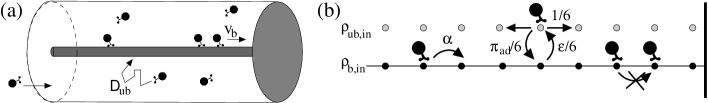
Figure 1: Motion of motor particles along a filament within a half-open tube (a) and the corresponding lattice model (b). At the left end, the system is connected to a motor reservoir with fixed bound and unbound densities $\rho_{\mathrm{b,in}}$ and $\rho_{\mathrm{ub,in}}$, while the right end is closed. Motor particles bound to the filament perform active movements with velocity $v_{\mathrm{b}}$, while unbound motors perform symmetric diffusion with diffusion constant $D_{\mathrm{ub}}$. In the lattice models, these movements are described by the forward step probability $\alpha$ on the filament and the symmetric hopping probability $1/6$ to each neighbour site for unbound motors. In addition, unbound motors which reach the filament bind to it with probability $\pi_{\mathrm{ad}}$, and bound motors unbind from the filament through steps to adjacent non-filament sites which occur with probability $\epsilon/6$ per non-filament neighbour site. The motors interact via hard core exclusion.

Each motor can be in two states: bound to the filament, where it moves actively to the right with velocity $v_{\mathrm{b}}$, and unbound, where it performs symmetric diffusion with diffusion constant $D_{\mathrm{ub}}$. The filament is taken to lie along the $x$-axis, so that the system is characterized by the bound motor density $\rho_{\mathrm{b}}(x)$ and the unbound motor density $\rho_{\mathrm{ub}}(x)$. As in [26, 28], we neglect the variation of the unbound motor density $\rho_{\mathrm{ub}}$ with the transverse coordinates $y$ and $z$.

The motors can unbind from or bind to the filament. Since the motors are strongly attracted by the filament, the binding rate $\pi_{0}$ is taken to be large compared to the unbinding rate $\epsilon_{0}$. When motors come close to each other, they may interact. In our simple model we include only hard core exclusion which prevents motors from occupying the same site. In a mean field treatment, this can be taken into account by using exclusion factors of the form $(1-\rho_{\mathrm{b}})$ or $(1-\rho_{\mathrm{ub}})$.

We are interested in the stationary states of the system. Since the right tube end is closed, the net current vanishes in the stationary state. Thus, the directed bound current of motors, $v_{\mathrm{b}}\rho_{\mathrm{b}}(1-\rho_{\mathrm{b}})$, and the unbound diffusive motor current, $-\phi D_{\mathrm{ub}}\frac{\partial}{\partial x}\rho_{\mathrm{ub}}$, must balance to give zero total current:

$$v_{\mathrm{b}}\rho_{\mathrm{b}}(1-\rho_{\mathrm{b}})-\phi D_{\mathrm{ub}}\frac{\partial}{\partial x}\rho_{\mathrm{ub}}=0.$$ (1)

Here the unbound diffusive current has been integrated over the tube cross section. The prefactor $\phi$ describes the area available for unbound diffusion. For large radii R, $\phi\approx\pi R^{2}$. Furthermore, in the stationary state, the in- and outgoing currents balance on any filament site which leads to

$$\frac{\partial}{\partial x}\left[v_{\mathrm{b}}\rho_{\mathrm{b}}(1-\rho_{\mathrm{b}})\right]=\pi_{0}\rho_{\mathrm{ub}}(1-\rho_{\mathrm{b}})-\epsilon_{0}\rho_{\mathrm{b}}(1-\rho_{\mathrm{ub}})$$ (2)

where the small diffusive part of the bound current has been neglected. The change of the bound current drives the system out of adsorption equilibrium for which the binding term $\pi_{0}\rho_{\mathrm{ub}}(1-\rho_{\mathrm{b}})$ and the unbinding term $\epsilon_{0}\rho_{\mathrm{b}}(1-\rho_{\mathrm{ub}})$ would be equal, i.e.

$$\pi_{0}\rho_{\mathrm{ub}}(1-\rho_{\mathrm{b}})=\epsilon_{0}\rho_{\mathrm{b}}(1-\rho_{\mathrm{ub}}).$$ (3)

For simplicity, we assume that the boundary densities at the left boundary, $\rho_{\mathrm{b,in}}$ and $\rho_{\mathrm{ub,in}}$, fulfill this adsorption equilibrium condition (3).

In addition to studying equations (1) and (2) by analytical approximations, we use Monte Carlo simulations of lattice models as in [6, 26] to obtain the stationary density and current profiles. In the simulations, the motors are represented by random walkers on a cubic lattice with lattice constant $\ell$, see figure 1(b). A line of lattice sites represents the filament. Motors at the filament sites perform a biased random walk, while motors at non-filament sites perform symmetric random walks. The jump probabilities per unit time $\tau$ are $\alpha$, $\beta$ and $\gamma$ for a forward, a backward and no step at filament sites, respectively, and $1/6$ for steps to each neighbour site at non-filament sites. In the following, we use $\beta=0$ for simplicity. Unbinding from the filament occurs with probability $\epsilon/6$ to each adjacent non-filament site, and unbound motors which reach the filament bind to it with probability $\pi_{\mathrm{ad}}$. Exclusion is implemented by rejecting all hopping attempts to sites which are already occupied by another motor. The hopping rates of the lattice models are matched to the transport properties of the motors via $\tau=\ell^{2}/(6D_{\mathrm{ub}})$, $v_{\mathrm{b}}=\alpha\ell$, $\pi_{0}=4\pi_{\mathrm{ad}}/6$ and $\epsilon_{0}=4\epsilon/6$, see [6, 26] and the appendix C in [7].

3 Steady states and relevant length scales

Figure 2: (a) Bound density profiles $\rho_{\mathrm{b}}$ and (b) current densities $j_{\mathrm{b}}$ for different boundary densities $\rho_{\mathrm{b,in}}$ as obtained from Monte Carlo simulation ($\diamondsuit$) and from the adsorption equilibrium approximation (solid lines). The parameters are $v_{\mathrm{b}}=-0.001$, $\epsilon_{0}=2/300$, $\pi_{0}=2/3$, $\phi=4$.

When the motors on the filament move to the right, i.e. for $v_{\mathrm{b}}>0$, they jam up at the closed right end until the tube far from the left boundary is completely filled with motors. In the bulk of a long tube, one thus has bound and unbound motor densities $\rho_{\mathrm{b}}=1$ and $\rho_{\mathrm{ub}}=1$. Indeed, these density values are a fixed point of equations (1) and (2). Within a boundary region at the left end, the densities cross over to the boundary values $\rho_{\mathrm{b,in}}$ and $\rho_{\mathrm{ub,in}}$.

Likewise, if the motors on the filament move to the left, i.e. for $v_{\mathrm{b}}<0$, they are driven out of the tube at the left end, so that the bulk is left empty with $\rho_{\mathrm{b}}=0$ and $\rho_{\mathrm{ub}}=0$, which is another fixed point of equations (1) and (2). However, a boundary region at the left end survives, fed by ingoing diffusion. Typical motor density profiles for this case are shown in figure 2(a). They display a ”jam” region at the left end, separated from the ”empty” bulk region by a localized domain wall or shock. The system is thus characterized by two length scales: the bulk length scale $\xi$ on which the densities approach their the bulk values and which is independent of the boundary densities, and the jam length $L_{*}$ which describes the width of the jammed boundary region and which, of course, strongly depends on the boundary densities.

On tuning the motor velocity $v_{\mathrm{b}}$, the system displays two phases, a high and a low density phase, which are dominated by the closed right end. Taking the bulk density as order parameter, one has a phase transition at $v_{\mathrm{b}}=0$. As will be shown both in analytical approximation and in Monte Carlo simulation, both characteristic length scales $\xi$ and $L_{*}$ diverge with the power law $1/v_{\mathrm{b}}$ as the motor velocity $v_{\mathrm{b}}$ approaches zero.

In an experiment, this limit can easily be realized by reducing the concentration [ATP] of the motor fuel ATP, since for small [ATP], $v_{\mathrm{b}}\sim$ [ATP]. Changing the sign of $v_{\mathrm{b}}$ is much more difficult, one possibility is to use motor particles driven by motors of two species with opposite directionality, so that one could invert the movement by activating one motor species while deactivating the other. If these motor particles switch stochastically between the two directions, one could change the sign of their average velocity by influencing the switching rates through regulatory molecules. For example, tau proteins which strongly suppress movements towards the synapse in axons can induce the retreat of vesicles into the cell body [33].

For $v_{\mathrm{b}}=0$, i.e. when there is no active motion of the motors, the system is in thermodynamic equilibrium, and the adsorption equilibrium as described by equation (3) is valid for all $x$ along the filament. Thus the bulk densities are $\rho_{\mathrm{b}}=\rho_{\mathrm{b,in}}$ and $\rho_{\mathrm{ub}}=\rho_{\mathrm{ub,in}}$. This case is the only one where the bulk values are dominated by the open left filament end. A phase diagram is shown in figure 3, the control parameters are the motor velocity $v_{\mathrm{b}}$ and the left boundary density $\rho_{\mathrm{b,in}}$.

Figure 3: Phase diagram for the half-open tube. For motors moving to the left, i.e. $v_{\mathrm{b}}<0$, the system is essentially empty with bulk density $\rho_{\mathrm{b}}=0$, while for motors moving to the right, i.e. $v_{\mathrm{b}}>0$, it is essentially full with bulk density $\rho_{\mathrm{b}}=1$. At the phase transition $v_{\mathrm{b}}=0$, the system is dominated by the left boundary density and has the bulk density $\rho_{\mathrm{b}}=\rho_{\mathrm{b,in}}$. For $v_{\mathrm{b}}<0$, the motors form a traffic jam with length $L_{*}$ at the left end, provided that the boundary density $\rho_{\mathrm{b,in}}$ is larger than $1/2$. Likewise, for $v_{\mathrm{b}}>0$ and $\rho_{\mathrm{b,in}}<1/2$, a ’jam of holes’, i.e. a region with low density, separates the (completely filled) bulk of the system from the left boundary.

To examine the bulk behaviour, equations (1) and (2) are linearized around the appropriate fixed point. In the case of motors moving to the left ($v_{\mathrm{b}}<0$) with bulk values $\rho_{\mathrm{b}}=\rho_{\mathrm{ub}}=0$, the linearization leads to an exponential density profile with

$$\rho_{\mathrm{b}}\approx\mathcal{N}\exp(-x/\xi)\quad\mathrm{and}\quad\rho_{\mathrm{ub}}\approx\left(\frac{\epsilon_{0}}{\pi_{0}}-\frac{v_{\mathrm{b}}}{\pi_{0}\xi}\right)\rho_{\mathrm{b}}$$ (4)

with the bulk length scale

$$\xi=2\Delta x_{\mathrm{b}}\left[1-\sqrt{1+4\left(\frac{\Delta x_{\mathrm{b}}}{\Delta x_{\mathrm{ub}}}\right)^{2}}\right]^{-1}\approx-\frac{(\Delta x_{\mathrm{ub}})^{2}}{\Delta x_{\mathrm{b}}}=-\frac{\epsilon_{0}}{\pi_{0}}\frac{\phi D_{\mathrm{ub}}}{v_{\mathrm{b}}},$$ (5)

where

$$\Delta x_{\mathrm{b}}=\frac{v_{\mathrm{b}}}{\epsilon_{0}}\quad\mathrm{and}\quad\Delta x_{\mathrm{ub}}=\sqrt{\frac{\phi D_{\mathrm{ub}}}{\pi_{0}}}$$ (6)

are the average walking distance on the filament before unbinding and the average diffusion distance before binding of a motor, respectively. The approximation in equation (5) is valid for small motor velocities $v_{\mathrm{b}}$. The exponential behaviour near the bulk value is in agreement with simulations.

In the case of motors moving to the right, the same reasoning leads to an exponential approach of the bulk values $\rho_{\mathrm{b}}=1$ and $\rho_{\mathrm{ub}}=1$ with the length scale

$$\xi=-2\Delta x_{\mathrm{b},\mathrm{h}}\left[1-\sqrt{1+4\left(\frac{\Delta x_{\mathrm{b},\mathrm{h}}}{\Delta x_{\mathrm{ub},\mathrm{h}}}\right)^{2}}\right]^{-1}\approx\frac{(\Delta x_{\mathrm{ub},\mathrm{h}})^{2}}{\Delta x_{\mathrm{b},\mathrm{h}}}=\frac{\pi_{0}}{\epsilon_{0}}\frac{\phi D_{\mathrm{ub}}}{v_{\mathrm{b}}}$$ (7)

where the last expressions are again valid for small motor velocity $v_{\mathrm{b}}$, and where $\Delta x_{\mathrm{b},\mathrm{h}}=v_{\mathrm{b}}/\pi_{0}$ and $\Delta x_{\mathrm{ub},\mathrm{h}}=\sqrt{\phi D_{\mathrm{ub}}/\epsilon_{0}}$ are the average walking distance on the filament before unbinding and the average diffusion distance before binding of a hole, respectively. This result can be obtained directly from (5) by exploring particle-hole symmetry, i.e. by substituting the left by the right boundary condition, $\rho_{\mathrm{b}}$ by $1-\rho_{\mathrm{b}}$, $\rho_{\mathrm{ub}}$ by $1-\rho_{\mathrm{ub}}$, $v_{\mathrm{b}}$ by $-v_{\mathrm{b}}$ and $x$ by $L-x$, and by exchanging $\pi_{0}$ and $\epsilon_{0}$.

According to equations (5) and (7) the bulk length scale $\xi$ diverges in the limit of small $v_{\mathrm{b}}$ with the power law $1/v_{\mathrm{b}}$. The same power law is obtained both if $v_{\mathrm{b}}=0$ is approached from above and from below, but with different amplitudes.

4 The jam region

In the following, we will focus on motors moving to the left, i.e. on the case $v_{\mathrm{b}}<0$. The case of motors moving to the right can easily be deduced as above by invoking particle-hole symmetry. Left-moving motors jam up in front of the left boundary, leading to a boundary dominated length scale in the system, the jam length $L_{*}$. In the jam region, the motors move slowly and thus ”have time” to equilibrate with the unbound motors before moving on. This separation of time scales leads to approximate adsorption equilibrium

$$\pi_{0}\rho_{\mathrm{ub}}(1-\rho_{\mathrm{b}})\approx\epsilon_{0}\rho_{\mathrm{b}}(1-\rho_{\mathrm{ub}})$$ (8)

at every filament site $x$.

4.1 Density profile and jam length

With the adsorption equilibrium approximation as given by equation (8), one can eliminate $\rho_{\mathrm{ub}}$ from the current balance equation (1) which leads to

$$\frac{\partial}{\partial x}\rho_{\mathrm{b}}=\frac{V}{L}\frac{(1-K)^{2}}{K}\rho_{\mathrm{b}}(1-\rho_{\mathrm{b}})\left(\frac{1}{1-K}-\rho_{\mathrm{b}}\right)^{2}$$ (9)

where the dimensionless constants

$$K=\frac{\epsilon_{0}}{\pi_{0}}\quad\mathrm{and}\quad V=\frac{Lv_{\mathrm{b}}}{\phi D_{\mathrm{ub}}}$$ (10)

have been introduced. The desorption constant $K$ is the ratio of unbinding to binding rate, while the dynamic constant $V$ is the ratio of the time $t_{\mathrm{ub}}=L^{2}/(\phi D_{\mathrm{ub}})$ needed to diffuse over the filament length $L$ to the time $t_{\mathrm{b}}=L/v_{\mathrm{b}}$ needed to walk this distance. Separation of variables, decomposition into partial fraction and subsequent integration of equation (9), using the boundary condition $\rho_{\mathrm{b}}(0)=\rho_{\mathrm{b,in}}$, leads to an implicit equation for the bound density $\rho_{\mathrm{b}}$:

$$\frac{x}{L}=\frac{1}{V}\left[g(\rho_{\mathrm{b}}(x),K)-g(\rho_{\mathrm{b,in}},K)\right].$$ (11)

The function

$$g(\rho,K)=\frac{-1}{\frac{1}{1-K}-\rho}+K\ln(\rho)-\frac{1}{K}\ln(1-\rho)+\frac{1-K^{2}}{K}\ln\left|\frac{1}{1-K}-\rho\right|$$ (12)

is a continuous, monotonically increasing, and thus invertible function for $0\leq\rho\leq 1$ and respects particle-hole symmetry which is equivalent to $g(1-\rho,1/K)=-g(\rho,K)$. In the jam region, the profiles obtained from equation (11) agree nicely with the Monte Carlo profiles, while they differ in the shock and the bulk region, where adsorption equilibrium is no longer a good approximation, see figure 2(a). In figure 2(b), we also show the corresponding profiles of the bound current $j_{\mathrm{b}}=v_{\mathrm{b}}\rho_{\mathrm{b}}(1-\rho_{\mathrm{b}})$ which exhibits a maximum close to the domain wall between the jammed and the bulk region.

Figure 4: Jam length $L_{*}$ as a function (a) of the boundary density $\rho_{\mathrm{b,in}}$ (with fixed velocity $v_{\mathrm{b}}=-0.001$) and (b) of the motor velocity $v_{\mathrm{b}}$ (with fixed $\rho_{\mathrm{b,in}}=0.9$). Both Monte Carlo ($\diamondsuit$) and analytic results (solid lines) from the jam region approximation (13) are shown. The other parameters are as in figure 2. In (a), we also display the averaged bound current $\overline{J}_{\mathrm{b}}$ as obtained from simulations ($\circ\,$) and from adsorption equilibrium approximation (17) with its maximum at $\rho_{\mathrm{b,in}}^{\max}$.

We therefore use the position of the current maximum as a definition for the jam length $L_{*}$. In the jam region the current is low due to a too high motor density while on the other side of the shock there are too few motors, also leading to a small current. As the maximal current is obtained for $\rho_{\mathrm{b}}=1/2$, the jam length $L_{*}$ is given by

$$\frac{L_{*}}{L}=\frac{1}{V}\left[g(\frac{1}{2},K)-g(\rho_{\mathrm{b,in}},K)\right].$$ (13)

Note that the jam length $L_{*}$ is positive only if $\rho_{\mathrm{b,in}}\geq 1/2$. For smaller boundary densities $L_{*}<0$ which implies that the domain wall is located outside the tube which then does not exhibit a motor traffic jam. The jam lengths determined from equation (13) are shown in figure 4 and agree well with the corresponding simulation results. As expected, the jam length increases with the boundary density $\rho_{\mathrm{b,in}}$. It diverges logarithmically, $L_{*}\approx L/(VK)\ln(1-\rho_{\mathrm{b,in}})$, as $\rho_{\mathrm{b,in}}$ approaches $1$ (of course this divergence is truncated by the finite system size). If the velocity $v_{\mathrm{b}}$ approaches zero, the jam length diverges as $1/v_{\mathrm{b}}$ and the jammed region spreads over the whole system in agreement with the fact that for $v_{\mathrm{b}}=0$ the left boundary dominates the whole system, as has been discussed in section 3 above. The exponent $-1$ of the divergence for $v_{\mathrm{b}}\rightarrow 0$, which has been obtained using mean field and adsorption equilibrium approximations, is confirmed by the Monte Carlo simulation results, see figure 4(b).

4.2 The case $K=1$

In the special case $K=1$, where binding to the filament and unbinding from the filament occur with the same rate, the implicit equation (11) for the density profile can be inverted and leads to the density profile

$$\rho_{\mathrm{b}}(x)=\left[1+\frac{1-\rho_{\mathrm{b,in}}}{\rho_{\mathrm{b,in}}}\;\exp\left({-V\frac{x}{L}}\right)\right]^{-1}.$$ (14)

The jam length $L_{*}$ in this case is given by

$$\frac{L_{*}}{L}=\frac{1}{V}\ln\left(\frac{1-\rho_{\mathrm{b,in}}}{\rho_{\mathrm{b,in}}}\right).$$ (15)

4.3 The average bound current

In order to characterize the overall transport in the system we consider the average bound current [6] which is defined by

$$\overline{J}_{\mathrm{b}}=\frac{1}{L}\int_{0}^{L}j_{\mathrm{b}}(\rho_{\mathrm{b}}(x))\,dx.$$ (16)

Since the bound density is essentially zero in the bulk, the bound current $j_{\mathrm{b}}(\rho_{\mathrm{b}})=v_{\mathrm{b}}\rho_{\mathrm{b}}(1-\rho_{\mathrm{b}})$ has large absolute values only in the boundary region near the left end. It is thus appropriate to use the jam region approximation of section 4.1 to calculate the average bound current $\overline{J}_{\mathrm{b}}$, which leads to

$$\frac{\overline{J}_{\mathrm{b}}}{v_{\mathrm{b}}}=\frac{1}{V}\frac{K}{(1-K)^{2}}\left[\frac{1}{\frac{1}{1-K}-\rho_{\mathrm{b}}(L)}-\frac{1}{\frac{1}{1-K}-\rho_{\mathrm{b,in}}}\right].$$ (17)

For large system size $L$ the right boundary density vanishes, and thus the average bound current is given by

$$\frac{\overline{J}_{\mathrm{b}}}{v_{\mathrm{b}}}\approx\frac{1}{V}\frac{K}{(1-K)}\left[1-\frac{1}{1-(1-K)\rho_{\mathrm{b,in}}}\right].$$ (18)

Interestingly, as $V\sim v_{\mathrm{b}}$, the current $\overline{J}_{\mathrm{b}}$ in the thermodynamic limit does not depend on the motor velocity $v_{\mathrm{b}}$. This is because the jam length $L_{*}$ decreases as $1/v_{\mathrm{b}}$, thus cancelling the expected $\overline{J}_{\mathrm{b}}\sim v_{\mathrm{b}}$ behaviour.

The average bound current from equation (17) agrees well with the current from the Monte Carlo simulation, see figure 4(a). As a function of the left boundary density $\rho_{\mathrm{b,in}}$, it displays a maximum absolute value at a density $\rho_{\mathrm{b,in}}^{\max}$. This density thus optimizes the motor transport in the system. It can be calculated via

$$0 = \frac{\partial\overline{J}_{\mathrm{b}}}{\partial\rho_{\mathrm{b,in}}}=\frac{1}{V}\left[j_{\mathrm{b}}\left(\rho_{\mathrm{b}}(L)\right)g^{\prime}(\rho_{\mathrm{b}}(L))\frac{\partial\rho_{\mathrm{b}}(L)}{\partial\rho_{\mathrm{b,in}}}-j_{\mathrm{b}}\left(\rho_{\mathrm{b,in}}\right)g^{\prime}(\rho_{\mathrm{b,in}})\right]$$ (19)

$$= \frac{1}{V}\left[j_{\mathrm{b}}\left(\rho_{\mathrm{b}}(L)\right)-j_{\mathrm{b}}\left(\rho_{\mathrm{b,in}}\right)\right]\,g^{\prime}(\rho_{\mathrm{b,in}}).$$

The last expression follows from

$$0=g^{\prime}(\rho_{\mathrm{b}}(L))\frac{\partial\rho_{\mathrm{b}}(L)}{\partial\rho_{\mathrm{b,in}}}-g^{\prime}(\rho_{\mathrm{b,in}})$$ (20)

which is obtained by differentiating (11), taken at $x=L$, with respect to $\rho_{\mathrm{b,in}}$. As $g^{\prime}(\rho_{\mathrm{b,in}})>0$ for $0\leq\rho_{\mathrm{b,in}}\leq 1$, a current extremum can occur only for

$$j_{\mathrm{b}}\left(\rho_{\mathrm{b,in}}\right)=j_{\mathrm{b}}\left(\rho_{\mathrm{b}}(L)\right).$$ (21)

Since equality of the densities at the left and right end occurs only for a completely full or completely empty tube, the condition for extremal current is

$$\rho_{\mathrm{b,in}}=1-\rho_{\mathrm{b}}(L).$$ (22)

Using this condition in equation (11) with $x=L$, one obtains the density that extremizes the average current from

$$V=g(\rho_{\mathrm{b,in}}^{\max})-g(1-\rho_{\mathrm{b,in}}^{\max})$$ (23)

The theoretical calculation agrees well with the simulation results, see figure 4. The current extremum occurs when the tube is approximately full, i.e. when the jam length $L_{*}$ is only slightly smaller than the tube length $L$. This is consistent with the assumption that the average current is mainly supported by the jam region, on which the use of the adsorption equilibrium approximation for the calculation of the average current is based.

In the limit of large $L$, one must thus jam up an infinite tube, for which one needs a boundary density $\rho_{\mathrm{b,in}}=1$. For this case, equation (23) can be inverted approximately which leads to

$$\rho_{\mathrm{b,in}}^{max}\approx 1-K^{\frac{1-K^{2}}{1+K^{2}}}\mathrm{e}^{\frac{-(1-K)^{2}}{1+K^{2}}}\exp{\left[-\frac{K}{1+K^{2}}\frac{|v_{\mathrm{b}}|}{D_{\mathrm{ub}}\phi}L\right]},$$ (24)

i.e. the maximum density $1$ is approached exponentially for large $L$.

5 Summary and conclusions

We have studied the molecular motor traffic in half-open tube-like compartments and characterized the traffic jams which result from the mutual exclusion of motors. In particular, we have obtained analytical results for the jam length and for the parameters which optimize the traffic in these compartments.

However, although the current within these compartments can be optimized, the stationary state of these half-open tubes is always characterized by a density which approaches either one or zero far from the open end (with a phase transition separating these two cases). Long tubes are therefore either essentially filled or essentially empty. In axons which are mimicked by this tube geometry, additional regulatory processes are therefore necessary to maintain efficient stationary transport.

These effects are not restriced to the tube geometry but apply generally to systems which are coupled to a particle reservoir at one end and which have two types of channels ’perpendicular’ to this surface, one with unsymmetric directed and one with symmetric diffusive transport.

Appendix A The closed tube

So far, the motion of motors in a half-open geometry has been considered. A related system is one with closed boundaries at both ends which has been studied in [6, 28]. In this case, motors cannot enter or leave the system, and the total number of motors within the tube is fixed:

$$N=\int_{0}^{L}\left[\rho_{\mathrm{b}}(x)+\phi\rho_{\mathrm{ub}}(x)\right]\,dx.$$ (25)

For this closed system, the same arguments as for the half-open system can be applied, however the integral constraint (25) makes the analysis more complicated.

Figure 5: (a) Density profiles $\rho_{\mathrm{b}}$ for the closed tube for various particle numbers $N$ as obtained from Monte Carlo simulations ($\diamondsuit$) and from the analytical jam region approximation (26) (solid lines). The parameters are $v_{\mathrm{b}}=1/300$, $\epsilon_{0}=2/300$, $\pi_{0}=2/3$ and $\phi=4$.
(b) Jam length $L_{*}$ ($\diamondsuit$) and average bound current $\overline{J}_{\mathrm{b}}$ ($\circ\,$) for the closed tube as functions of the number $N$ of motors within the tube. The data points are from simulations, the lines display the corresponding results from the adsorption equilibrium approximation as given by equations (26) and (30), respectively. The other parameters are as in (a).

Typical profiles for the closed system and motors moving to the right ($v_{\mathrm{b}}>0$) are displayed in figure 5(a). The profiles show the same two characteristic length scales as in the case of the half-open system: the bulk length $\xi$ and the jam length $L_{*}$. The bulk length $\xi$ which is independent of the boundary densities is again given by equation (5).

Depending on their direction of motion, the motors jam up at one of the closed ends. In this region, the motors move slowly, and the adsorption equilibrium approximation (8) can be applied which leads again to an implicit equation for the bound density:

$$\frac{x}{L}=\frac{1}{V}\left[g(\rho_{\mathrm{b}}(x),K)-g(\rho_{\mathrm{b}}(0),K)\right]$$ (26)

with the function $g$ as defined in equation (12). This equation corresponds to equation (11), however, the left boundary density $\rho_{\mathrm{b}}(0)$ is now unknown. It can be determined from the particle conservation constraint (25), which for adsorption equilibrium can be integrated and leads to:

$$V\frac{N}{L(1+\phi)}=F(\rho_{\mathrm{b}}(L),K,\phi)-F(\rho_{\mathrm{b}}(0),K,\phi)$$ (27)

with the function

$$F(\rho,K,\phi)=\frac{1}{K}\ln\left[\frac{\left|\frac{1}{1-K}-\rho\right|}{1-\rho}\right]-\frac{1}{1-(1-K)\rho}\left[1+\frac{K}{2}\frac{\phi}{1+\phi}\frac{1}{1-(1-K)\rho}\right].$$ (28)

Together with

$$V=g\left(\rho_{\mathrm{b}}(L),K)\right)-g\left(\rho_{\mathrm{b}}(0),K\right)$$ (29)

(obtained from equation (26) by setting $x=L$) one has two nonlinear equations for the boundary densities $\rho_{\mathrm{b}}(0)$ and $\rho_{\mathrm{b}}(L)$, which are needed in equation (26). The resulting density profiles agree well with the Monte Carlo profiles in the jam region, see figure 5(a).

The average bound current and its maximum can be calculated in the same way as for the half-open tube, leading to:

$$\frac{\overline{J}_{\mathrm{b}}}{v_{\mathrm{b}}}=\frac{1}{V}\frac{K}{(1-K)^{2}}\left[\frac{1}{\frac{1}{1-K}-\rho_{\mathrm{b}}(L)}-\frac{1}{\frac{1}{1-K}-\rho_{\mathrm{b}}(0)}\right]$$ (30)

with an extremum as function of the particle number $N$ at

$$j_{\mathrm{b}}\left(\rho_{\mathrm{b}}(0)\right)=j_{\mathrm{b}}\left(\rho_{\mathrm{b}}(L)\right)\quad\mathrm{or}\quad\rho_{\mathrm{b}}(0)=1-\rho_{\mathrm{b}}(L).$$ (31)

Thus, from equation (27), the maximum occurs for the particle number

$$\frac{N^{\max}}{L(1+\phi)}=\frac{1}{V}\left[F(1-\rho_{\mathrm{b}}(L))-F(\rho_{\mathrm{b}}(L))\right].$$ (32)

The results for the average current agree quite well with the simulation results, see figure 5(b). Only near the current extremum the Monte Carlo curve is slightly sharper than the curve from the adsorption equilibrium approximation which leads to a different value for the current extremizing particle number $N^{\max}$.

For a very long tube, the current extremum occurs at particle number

$$\frac{N^{\max}}{L(1+\phi)}\approx\frac{1}{1+K^{2}}\left(1+\frac{1}{L}\frac{D_{\mathrm{ub}}\phi}{v_{\mathrm{b}}}h(K,\phi)\right)$$ (33)

with $h(K,\phi)=\frac{(1-K)^{2}}{K}-\frac{1}{K}\ln{K}-\frac{(1-K)(1+K^{2})}{2K}\frac{2+(3+K)\phi}{1+\phi}$, and thus approaches $\frac{1}{1+K^{2}}$ for large $L$.

References

- [1] Alberts B, Johnson A, Lewis J, Raff M, Roberts K and Walter P 2002 Molecular Biology of the Cell 4th edition (New York and London: Garland)
- [2] Schliwa M and Woehlke G 2003 Molecular motors Nature 422 759–765
- [3] Goldstein L S B and Yang Z 2000 Microtubule-based transport systems in neurons: The roles of kinesins and dyneins. Annu. Rev. Neurosci. 23 39–71
- [4] Howard J 2001 Mechanics of Motor Proteins and the Cytoskeleton (Sunderland: Sinauer Associates)
- [5] Schliwa M 2003 Molecular motors (Weinheim: Wiley-VCH)
- [6] Lipowsky R, Klumpp S and Nieuwenhuizen T M 2001 Random walks of cytoskeletal motors in open and closed compartments Phys. Rev. Lett. 87 108101
- [7] Lipowsky R and Klumpp S 2005 ’Life is motion’ – multiscale motility of molecular motors Physica A 352 53–112
- [8] Ajdari A 1995 Transport by active filaments Europhys. Lett. 31 69–74
- [9] Howard J, Hudspeth A J and Vale R D 1989 Movement of microtubules by single kinesin molecules Nature 342 154–158
- [10] Svoboda K, Schmidt Ch F, Schnapp B J and Block S M 1993 Direct observation of kinesin stepping by optical trapping interferometry Nature 365 721–727
- [11] Vale R D, Funatsu T, Pierce D W, Romberg L, Harada Y and Yanagida T 1996 Direct observation of single kinesin molecules moving along microtubules Nature 380 451–453
- [12] Visscher K , Schnitzer M J and Block S M 1999 Single kinesin molecules studied with a molecular force clamp Nature 400 184–189
- [13] Jülicher F, Ajdari A and Prost J 1997 Modeling molecular motors Rev. Mod. Phys. 69 1269–1281
- [14] Lipowsky R 2000 Molecular motors and stochastic models Stochastic processes in physics, chemistry and biology ed J A Freund and T Pöschel (Berlin: Springer) pp 21–31
- [15] Astumian R D and Hänggi P 2002 Brownian motors Physics Today 55(11) 33–39
- [16] Qian H 1997 A simple theory of motor protein kinetics and energetics Biophys. Chem. 67 263–267
- [17] Fisher M E and Kolomeisky A B 1999 The force exerted by a molecular motor Proc. Natl. Acad. Sci. USA 96 6597–6602
- [18] Lipowsky R 2000 Universal aspects of the chemomechanical coupling for molecular motors Phys. Rev. Lett. 85 4401–4405
- [19] Lipowsky R and Jaster N 2003 Molecular motor cycles: From ratchets to networks J. Stat. Phys. 110 1141–1167
- [20] Nieuwenhuizen T M, Klumpp S and Lipowsky R 2002 Walks of molecular motors in two and three dimensions Europhys. Lett. 58 468–474
- [21] Nieuwenhuizen T M, Klumpp S and Lipowsky R 2004 Random walks of molecular motors arising from diffusional encounters with immobilized filaments Phys. Rev. E 69 061911
- [22] Katz S, Lebowitz J L and Spohn H 1983 Phase transitions in stationary nonequilibrium states of model lattice systems Phys. Rev. B 28 1655–1658
- [23] Krug J 1991 Boundary-induced phase transitions in driven diffusive systems Phys. Rev. Lett. 67 1882–1885
- [24] Schütz G M 2001 Exactly solvable models for many-body systems far from equilibrium Phase Transitions and Critical Phenomena vol 19 ed C Domb and J L Lebowitz (San Diego: Academic Press) pp 1–251
- [25] Chowdhury D, Santen L and Schadschneider A 2000 Statistical physics of vehicular traffic and some related systems Phys. Rep. 329 199–329
- [26] Klumpp S and Lipowsky R 2003 Traffic of molecular motors through tube-like compartments J. Stat. Phys. 113 233–268
- [27] Klumpp S and Lipowsky R 2004 Phase transitions in systems with two species of molecular motors Europhys. Lett. 66 90–96
- [28] Klumpp S, Nieuwenhuizen T M and Lipowsky R 2005 Self-organized density patterns of molecular motors in arrays of cytoskeletal filaments Biophys. J. 88 3118–3132
- [29] Parmeggiani A, Franosch T and Frey E 2003 Phase coexistence in driven one dimensional transport Phys. Rev. Lett. 90 086601
- [30] Popkov V, Rákos A, Willmann R D, Kolomeisky A B and Schütz G M 2003 Localization of shocks in driven diffusive systems without particles number conservation Phys. Rev. E 67 066117
- [31] Evans M R, Juhász R and Santen L 2003 Shock formation in an exclusion process with creation and annihilation Phys. Rev. E 68 026117
- [32] Klein G, Kruse K, Cuniberti G and F. Jülicher F 2005 Filament depolymerization by motor molecules Phys. Rev. Lett. 94 108102
- [33] Mandelkow E-M, Thies E, Trinczek B, Biernat J and Mandelkow E 2004 MARK/PAR1 kinase is a regulator of microtubule-dependent transport in axons J. Cell Biol. 167 99–110