Slow Vibrations in Transport through Molecules

Abstract

We show how one can measure the signal from slow jumps of a single molecule between metastable positions using a setup where the molecule is fixed to one lead, and one of the coupling strengths is controlled externally. Such a measurement yields information about slow processes deforming the molecule in times much longer than the characteristic time scales for the electron transport process.

One of the key ideas in studies of electron transport through single molecules is the aim to relate the properties of the studied microscopic molecule to the current flowing through it. Then measuring this current will yield information about the molecule. There are many interesting transport phenomena, known from larger structures, e.g., semiconductor quantum dots, that have been also observed in molecules park02 ; liang02 ; kubatkin03 . However, perhaps a feature most specific to the molecular systems is the large signature of the mechanical vibrations on the transport properties. Such effects include the electron shuttling fedorets04 and polaronic effects flensberg ; galperin05 , e.g., the vibration-assisted electron tunneling effect, observed through the side peaks in the differential conductance stipe98 ; park00 ; smit02 ; pasupathy05 at positions corresponding to the vibrational frequencies. Another molecule-specific property can be seen when one is able to vary the coupling of the molecule to the leads between weak and strong coupling limits grueter05 . In this case, one can quantitatively characterize the different coupling strengths, by fitting the experimentally measured conductance to a fairly generic model describing transport through the closest molecular level(s). Such a model relies on the fact that the molecule is coupled to the leads only from one side, allowing one to tune the other coupling over a wide range. From this fit, one then obtains four molecule-specific parameters corresponding to the two coupling strengths at given positions, an energy scale describing the position of the HOMO/LUMO level (whichever is closer) and a length scale describing the change of the coupling as a function of the distance. These parameters can then be used as a fingerprint of that particular molecule.

The typically considered vibrational effects are characteristic of weak coupling for the electron hopping between the leads and the molecule, in which case the vibrational frequency scales exceed or are of the same order as the coupling strength. In such systems, it is essential to consider the fairly fast and low-amplitude vibrations inside a single parabolic confining potential around some long-lived metastable position. However, on a much slower scale, the molecule may jump between different metastable states corresponding to different conformations or positions. Our aim is to discuss in this paper how these jumps may be observed and characterized.

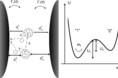
Figure 1: Schematic illustration of the considered situation: Left: A small molecule is connected to the left lead via a linker (this particular molecule is from Ref. grueter05, ). Due to the coupling via a single linker, the molecule-linker-lead system has multiple metastable configurations, corresponding to different positions. The distances $d_{L}^{i}$ and $d_{R}^{i}$ to the two leads are also indicated. Right: A possible potential profile corresponding to the position of the molecule, shown in the left figure by the coordinate $x$. Due to the directional character of the bonding to the leads, due to the solvent, or due to the particular atomic arrangement of the left lead, there may be a few metastable configurations indicated by the potential minima. The hopping between these configurations depends on the heights $U_{1}$ and $U_{2}$ of the potential barrier. If $U_{1}\neq U_{2}$, the probability $p_{1}$ to occupy state $1$ is larger than the corresponding probability $p_{2}$ for state 2.

Consider a potential energy curve depicted in Fig. 1. The horizontal axis could quantify different molecular conformations or average positions. The vibrations within a single potential well are governed with a frequency $\omega_{k}=\sqrt{k/m}$, where $k$ is the spring constant describing the potential and $m$ is the mass of the molecule. Brownian motion of the particle within this potential well at the temperature $T$ will then result into vibrations with amplitude $s\sim\sqrt{k_{B}T/k}$. The amplitude of such vibrations is much smaller than the distance between successive potential minima, and hence it is at most of the order of a few ${\mathrm{\AA}}$. We can use this as an estimate for the frequency $\omega_{k}$. At room temperature, for the case of a molecule with mass of the order of 1000 $\dots$ 10000 $m_{p}$, we would thus get $\omega_{k}\gtrsim 0.1\dots 1$ THz. These vibrations are damped by a friction force described by the characteristic rate $\gamma_{f}=c\eta R/m$, where $c$ is a constant of order unity depending on the shape of the molecule ($c=6\pi$ for a spherical molecule), $R$ characterizes the size of the molecule, and $\eta$ is the viscosity describing the molecule environment. For a spherical molecule of size $R\sim 1$nm, mass as given above and using the viscosity of water, $\eta$=1 g/(ms), we would thus get $\gamma_{f}\sim 10$ THz. Note that in practice, the effective viscosity of the solvent depends also on the molecule itself and thus this number should be used as indicative only. The jumps between the different potential minima have a much lower rate than the small-scale vibrations. This rate is described by the Arrhenius law, haenggi90

$$\gamma=\nu\exp(-\frac{U_{1}}{k_{B}T}),$$ (1)

where $U_{1}$ describes the height of the potential barrier (see Fig. 1), $\nu=\frac{\omega_{c}}{\gamma_{f}}\frac{\omega_{k}}{2\pi}$ in the overdamped limit $\gamma_{f}\gg\omega_{c}$ and $\nu=\omega_{k}/(2\pi)$ for $\omega_{k}\gg\gamma_{f}$. Here $\omega_{c}$ describes the width of the potential barrier, and is of the same order as $\omega_{k}$. With the above estimates for the frequencies $\omega_{k}$, $\omega_{c}$ and $\gamma_{f}$, the prefactor $\nu$ thus ranges from GHz to THz. However, the exponential factor makes the jumps between different minima much less frequent. Assume for example a potential barrier height of $U\approx 0.5$ eV bindingenergynote . At room temperature, we would then get $\gamma=\nu\exp(-20)$; ranging between Hz and kHz. This is close to the characteristic scale in which the measurements on the molecules are made and indeed such measurements grueter05 showed large fluctuations in the measured conductance, clearly connected to the presence of the molecule.

The distance-dependent linear conductance $G=G_{0}T$ through a single molecular level can be described by the Breit-Wigner formula datta ,

$$T=\frac{\Gamma_{L}\Gamma_{R}}{\epsilon_{1}^{2}+(\Gamma_{L}+\Gamma_{R})^{2}/4}.$$ (2)

Here $G_{0}=2e^{2}/h$, $\epsilon_{1}$ is the energy of the closest molecular level to the metal Fermi energy (i.e., LUMO or HOMO, whichever is closer) assuming it has an appreciable coupling to the leads, and $\Gamma_{L}$ and $\Gamma_{R}$ characterize the coupling to the left and right leads, respectively. The level $\epsilon_{1}$ may be degenerate - this degeneracy would only tune the effective coupling strengths $\Gamma_{L}$ and $\Gamma_{R}$ compared to the non-degenerate case. For simplicity, we neglect interaction effects. This assumption still captures the essential physics in the strong-coupling regime where the coupling energy $\Gamma_{L}+\Gamma_{R}$ exceeds the thermal energy and thus describes the lifetime of the level. Moreover, additional molecular levels may be considered, but their contribution shows up mostly to slightly rescale the coupling constants heikkilaup .

Consider now what happens if the molecule is connected to one of the leads, say left, thus fixing the average $\Gamma_{L}$. Assume furthermore $\Gamma_{L}\ll\epsilon_{1}$. The average coupling to the right lead depends on the distance $d_{R}$ between the molecule and the furthermost atom of this lead through $\Gamma_{R}=\Gamma_{R}^{*}\exp(-\kappa d_{R})$, where $\kappa$ depends on the solvent and on the molecule/lead materials grueterup05 . For $\Gamma_{R}\ll\epsilon_{1}$, decreasing $d_{R}$ will increase the conductance. However, when the right lead is close enough, $\Gamma_{R}$ may exceed the level energy $\epsilon_{1}$. In this case, the conductance shows a maximum at $\Gamma_{R}=\sqrt{4\epsilon_{1}^{2}+\Gamma_{L}^{2}}\approx 2\epsilon_{1}$ and further decrease of $d_{R}$ leads to a decrease in the conductance. This type of a model was employed to explain the observed conductance-distance curve in Ref. grueter05, with a quantitative agreement between the theory and the measured average conductance.

Consider now the fluctuation of this conductance, due to the slow hoppings of the molecule between different average positions. Such hopping corresponds to a random telegraph noise in a time-dependent signal. Let us denote the average distance between the right lead and the molecule by $d$ (average meaning averaging over the different positions of the molecule corresponding to the given positions of the leads). Let us furthermore choose the coupling strengths corresponding to this average position to $\overline{\Gamma}_{L}$ and $\overline{\Gamma}_{R}=\Gamma_{R}^{*}\exp(-\kappa d)$. Then, the fluctuations of the position around this average position can be characterized by the values $\{\delta d^{i},-c_{i}\delta d^{i}\}$, $i$ indexing the different potential minima, and the two numbers corresponding to the deviations of the distance to the left and right leads, respectively. In a typical case, one could expect that if the molecule moves further from the left lead ($\delta d>0$), it comes closer to the right lead (as in Fig. 1). This would thus correspond to a positive $c_{i}$. However, for certain situations it may be possible to increase the distance to both leads - this would be described with a negative $c_{i}$. With these deviations, the couplings change to $\Gamma_{L}^{i}=\overline{\Gamma}_{L}\exp(\kappa\delta d^{i})$ and $\Gamma_{R}^{i}=\overline{\Gamma}_{R}\exp(-\kappa c_{i}\delta d^{i})$. Note that choosing the same $\kappa$ for both $\Gamma_{L}$ and $\Gamma_{R}$ does not mean a lack of generality, as a possible difference in the two $\kappa$’s can be included to scale $c_{i}$.

The transmission averaged over the positions of the molecule is

$$\langle T\rangle=\sum_{i}p_{i}T_{i}\equiv\sum_{i}p_{i}\frac{\Gamma_{L}^{i}\Gamma_{R}^{i}}{\epsilon_{1}^{2}+(\Gamma_{L}^{i}+\Gamma_{R}^{i})^{2}/4}.$$ (3)

Here $p_{i}$ is the probability for the molecule to be in the position/configuration $i$. Thus, already the average transmission $\langle T\rangle$ depends on the amplitude $\delta d^{i}$ of fluctuations (see Fig. 2). However, such a dependence is difficult to see in $\langle T\rangle$, as a similar behavior could be observed also without vibrations, but with a slight rescaling of $\overline{\Gamma}_{L/R}$.

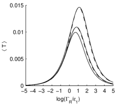
Figure 2: Average transmission as a function of coupling $\Gamma_{R}$ for different amplitudes of variations $\delta d$. The coupling $\Gamma_{R}$ can be varied by varying the distance between the electrodes, and the transmission peak details information about the molecule and its coupling to the leads. The hopping between different metastable configurations corresponding to different $\delta d$ affects the transmission: from top to bottom, $\delta d=0$ (no hopping), $\delta d=0.5/\kappa$ and $\delta d=1/\kappa$. We chose $\bar{\Gamma}_{L}=0.01\epsilon_{1}$ and $c=0.5$ and describe hopping between two degenerate configurations (i.e., with equal probabilities) separated from the average position by $\pm\delta d$. The dashed lines indicate fits to the Breit-Wigner transmission with no account of the fluctuations, but with an increased $\Gamma_{L}$ and a smaller $\Gamma_{R}^{*}$.

The variance of the transmission values due to these slow fluctuations is $\operatorname{var}(T)=\langle(T-\langle T\rangle)^{2}\rangle$. Assuming we can neglect the electronic noise (see below) which also shows up as a temporal variation of the current, this $\operatorname{var}(T)$ would vanish without the vibrations. In general, $\operatorname{var}(T)$ depends on $d$, the separation of the leads. However, if we assume that the positions of the metastable states with respect to the left lead are independent of $d$, we can separate two limits in the $d$-dependence. One is the case when $d$ is large, such that $\Gamma_{R}\ll\epsilon_{1}$. If also $\Gamma_{L}\ll\epsilon_{1}$, we can neglect the lifetime of the level (the term $\Gamma_{L}+\Gamma_{R}$ in the denominator of $T_{i}$). Then

$$T_{i}\overset{\Gamma\ll 2\epsilon_{1}}{\rightarrow}\frac{\Gamma_{L}^{i}\Gamma_{R}^{i}}{\epsilon_{1}^{2}}=\frac{\overline{\Gamma}_{L}\overline{\Gamma}_{R}}{\epsilon_{1}^{2}}\exp(\kappa(1-c_{i})\delta d^{i}).$$ (4)

Thus, the transmission probability for each $i$ can be written in a form $T_{i}=\overline{T}T_{f1}^{i}$, where $\overline{T}$ is independent of the random hoppings, but depends on the position $d$, and $T_{f1}^{i}$ depends on the hoppings, but not on the position $d$. In this case, we may express the relative variance as

$$\begin{split}&\sigma_{T}^{2}\equiv\frac{\operatorname{var}(T)}{\langle T\rangle^{2}}=\frac{\operatorname{var}(T_{f1}^{i})}{\langle T_{f1}^{i}\rangle^{2}}\\ &=\frac{\sum_{i}p_{i}\left\{\exp[\kappa\delta d_{i}(1-c_{i})]-\sum_{j}p_{j}\exp[\kappa\delta d_{j}(1-c_{j})]\right\}^{2}}{\left\{\sum_{j}p_{j}\exp[\kappa\delta d_{j}(1-c_{j})]\right\}^{2}}.\end{split}$$ (5)

Thus, this quantity no longer depends on the exact value of $d$, as long as $\overline{\Gamma}_{L}+\overline{\Gamma}_{R}\ll 2\epsilon_{1}$.

The same happens in the opposite limit, $\overline{\Gamma}_{R}\gg 2\epsilon_{1}$. In this case, we can neglect all other terms but $\Gamma_{R}$ from the denominator of the transmission and

$$T_{i}\overset{\Gamma_{R}\gg 2\epsilon_{1}}{\rightarrow}\frac{4\Gamma_{L}^{i}}{\Gamma_{R}^{i}}=\frac{\overline{\Gamma}_{L}}{\overline{\Gamma}_{R}}\exp(\kappa(1+c_{i})\delta d^{i})\equiv\bar{T}T_{f2}^{i}.$$ (6)

The relative fluctuations $\sigma_{T}$ again follow Eq. (5), with the only exception that the sign of each $c_{i}$ is reversed.

If the sign of $c_{i}$ is predominantly positive, $\sigma_{T}$ in the case $\Gamma_{R}\gg 2\epsilon_{1}$ will be larger than in the case $\Gamma\ll 2\epsilon_{1}$ and vice versa for a predominantly negative $c_{i}$. Thus, we can sketch the rough behavior of $\sigma_{T}$ as a function of the distance $d$ (assuming $c>0$): At first, when the leads are far apart, $\sigma_{T}$ stays mostly constant. When $\overline{\Gamma}_{R}$ becomes of the order of $2\epsilon_{1}$, $\sigma_{T}$ starts to increase with $d$, until saturating into another constant value at $\overline{\Gamma}_{R}\gg 2\epsilon_{1}$ (see Fig. 3). Such a behavior holds as long as the metastable positions of the molecule are unaffected by the right lead. The latter type of a mechanical effect would show up also in the average conductance curves if the right lead changes the potential landscape seen by the molecule. This was probably observed in Ref. grueter05, , but only when $\bar{\Gamma}_{R}$ was already much larger than $\epsilon_{1}$.

Figure 3: Relative variance in the measured conductance curves, observed as time-dependent fluctuations. The two solid lines are for hopping between two degenerate configurations with $\kappa\delta d=0.5$ (bottom) and $\kappa\delta d=1$ (top), and the dashed curve represents the case with four degenerate configurations, at $\delta d=\pm 0.5/\kappa$ and $\delta d=\pm 1/\kappa$. We chose $c=0.5$ for each curve.

To explore this behavior explicitly, let us consider a simple two-position model with the positions $\{\delta d/2,-c\delta d/2\}$ and $\{-\delta d/2,c\delta d/2\}$. In this case, we get a fairly simple expression for $\sigma_{T}$ in the limit $\overline{\Gamma}_{L}\ll\epsilon_{1}$,

$$\sigma_{T}=\left|\frac{4\epsilon_{1}^{2}\sinh(\kappa(1-c)\delta d/4)+\overline{\Gamma}_{R}^{2}\sinh(\kappa(1+c)\delta d/4)}{4\epsilon_{1}^{2}\cosh(\kappa(1-c)\delta d/4)+\overline{\Gamma}_{R}^{2}\cosh(\kappa(1+c)\delta d/4)}\right|.$$ (7)

In the limit $\Gamma_{R}\ll 2\epsilon_{1}$, this gives

$$\sigma_{T}\overset{\Gamma_{R}\ll 2\epsilon_{1}}{\rightarrow}|\tanh(\kappa(1-c)\delta d/4)|,$$ (8)

and in the opposite limit $\Gamma_{R}\gg 2\epsilon_{1}$,

$$\sigma_{T}\overset{\Gamma_{R}\gg 2\epsilon_{1}}{\rightarrow}|\tanh(\kappa(1+c)\delta d/4)|.$$ (9)

These limits follow the qualitative discussion above.

Apart from hopping between different positions, in some cases one may also envisage the molecule to hop between different conformations on the slow time scales. Such a change in the conformation in general may lead to a change both in the energy level $\epsilon_{1}$ and in the coupling strengths $\Gamma_{L/R}$. This behavior can be illustrated by considering the simplest case of hopping between two conformations corresponding to the energies $\epsilon_{1}\pm\delta\epsilon/2$ and couplings $\Gamma_{L}\pm\delta\Gamma_{L}/2$, $\Gamma_{R}\pm\delta\Gamma_{R}/2$. The relative variance $\sigma_{T}$ now depends on the relative magnitude of these changes: if $\delta\Gamma_{L/R}/(\Gamma_{L}+\Gamma_{R})\gg\delta\epsilon/\epsilon_{1}$, the behavior is analogous to that discussed above. In the opposite limit of large $\delta\epsilon$, the relative variance of the conductance values $\sigma_{T}=\operatorname{var}(T)/\langle T\rangle^{2}$ is given by

$$\sigma_{T}=\frac{16\delta\epsilon^{2}\epsilon_{1}^{2}}{(\delta\epsilon^{2}+(\Gamma_{L}+\Gamma_{R})^{2}+4\epsilon_{1}^{2})^{2}}.$$ (10)

Thus, the relative variance is largest when the couplings are much smaller than the level energies, and it decreases as either of the couplings is increased. A similar conclusion can be drawn for the general case with many different conformations, along the same arguments as above.

There are a few experimental constraints for the observation of the predicted behavior in the fluctuations, characterized by the different time scales in the problem. An easily satisfied condition is that the measurement time $\tau_{m}$ should exceed the time scales $1/\omega_{k}$, $\hbar/\Gamma_{L/R}$, $\tau_{e}=e/\langle I\rangle$ characterizing the individual charge transport processes (typically between ps and ns) by a few orders of magnitude. Here $\langle I\rangle$ is the average current through the molecule. In this limit, shot noise yields a contribution $\sim e/(\tau_{m}\langle I\rangle)=\tau_{e}/\tau_{m}$ to the relative variance and can hence be neglected. The same applies for the thermal noise provided that $k_{B}T/(eV)\tau_{e}/\tau_{m}\ll\sigma_{T}$, where $V$ is the bias voltage applied over the sample. Another natural condition is that the time scale $\tau_{\rm var}$ for the variations made in the structure (like changing the distance between the leads) should be longer than $\tau_{m}$ and the time scale $\tau_{\rm hops}=1/\gamma$ for the slow changes in the configurations. To obtain a relative accuracy $p$ for the measured variance, one has to measure at least $\sim 1/p^{2}$ points and therefore $\tau_{\rm var}/\tau_{m}>1/p^{2}$.

If there are only a few metastable configurations in the problem, and the time scales for hopping between them is longer than the measurement time, one may be able to measure the information about them already by following the telegraph noise in the average transmission as a function of time. However, for many configurations, or if at least some of the hopping time scales are smaller than $\tau_{m}$, it is better to measure the relative variance. When $\tau_{m}$ and $\tau_{\rm hops}$ are well separated, the measured variance in the signal will be proportional to

$$\operatorname{var}(G)_{m}=\operatorname{var}(G)_{c}\frac{\min(\tau_{m},\tau_{\rm hops})}{\max(\tau_{m},\tau_{\rm hops})}.$$ (11)

Here $\operatorname{var}(G)_{m}$ is the measured variance and $\operatorname{var}(G)_{c}=G_{0}^{2}\operatorname{var}(T)$ is the variance calculated above. In the case when there are multiple time scales describing the slow fluctuations, and the measurement time is between these scales, the measured variance will be independent of $\tau_{m}$, characteristic for flicker noise.

Summarizing, in this paper we predict that the different metastable atomic configurations in molecular junctions have a considerable effect in the measured conductance, as the time scale of typical conductance measurements is of the same order as the time scales for the jumps between the different configurations. We utilize a simple Breit-Wigner model to illustrate this behavior and show that such variations lead to a fairly universal behavior in the relative variance of the measured conductance values as one of the coupling constants between the molecule and the leads is controlled.

We thank Christoph Bruder, Michel Calame, Lucia Grüter and Christian Schönenberger for discussions that motivated this paper. This work was supported by the Swiss NSF and the NCCR Nanoscience.

References

- (1) J. Park, A. N. Pasupathy, J. I. Goldsmith, C. Chang, Y. Yaish, P. J. R., M. Rinkoski, J. P. Sethna, H. D. Abruna, P. L. McEuen, and D. C. Ralph, Nature 417, 722 (2002).
- (2) W. Liang, M. P. Shores, M. Bockrath, J. R. Long, and H. Park, Nature 417, 725 (2002).
- (3) S. Kubatkin, A. Danilov, M. Hjort, J. Cornil, J.-L. Bredas, N. Stuhr-Hansen, P. Hedegård, and T. Bjornholm, Nature 425, 698 (2003).
- (4) D. Fedorets, L. Y. Gorelik, R. I. Shekter, and M. Jonson, Phys. Rev. Lett. 92, 166801 (2004).
- (5) K. Flensberg, Phys. Rev. B 68, 205323 (2003); S. Braig and K. Flensberg, ibid 68, 205324 (2003).
- (6) M. Galperin, M. A. Ratner, and A. Nitzan, Nano Lett. 5, 125 (2005).
- (7) B. C. Stipe, M. A. Rezaei, and W. Ho, Science 280, 1732 (1998).
- (8) H. Park, J. Park, A. K. L. Lim, E. H. Anderson, A. P. Alivisatos, and P. L. McEuen, Nature 407, 57 (2000).
- (9) R. H. M. Smit, Y. Noat, C. Untiedt, N. D. Lang, M. C. van Hemert, and J. M. van Ruitenbeek, Nature 419, 906 (2002).
- (10) A. N. Pasupathy, et al., Nano Lett. 5, 203 (2005).
- (11) L. Grüter, F. Cheng, T. T. Heikkilä, M. T. Gonzalez, F. Diederich, C. Schönenberger, and M. Calame, Nanotechnology 16, 2143 (2005).
- (12) P. Hänggi, P. Talkner, and M. Borkovec, Rev. Mod. Phys. 62, 251 (1990).
- (13) S. Datta, Nanotechnology 15, S433 (2004).
- (14) T. T. Heikkilä, C. Schönenberger and W. Belzig, in preparation.
- (15) This could arise due to the energy difference in the different arrangements of the contacting atoms, for typical energy scales in the case of gold clusters, see J. Zhao, J. Yang, and J. G. Hou, Phys. Rev. B 67, 085404 (2003).
- (16) L. Grüter, M. T. Gonzalez, R. Huber, M. Calame, and C. Schönenberger, Small 1, 1067 (2005).