Electronic Structure Calculations with Dynamical Mean–Field Theory: A Spectral Density Functional Approach

Abstract

We present a review of the basic ideas and techniques of the spectral density functional theory which are currently used in electronic structure calculations of strongly–correlated materials where the one–electron description breaks down. We illustrate the method with several examples where interactions play a dominant role: systems near metal–insulator transition, systems near volume collapse transition, and systems with local moments.

I Introduction

Theoretical understanding of the behavior of materials is a great intellectual challenge and may be the key to new technologies. We now have a firm understanding of simple materials such as noble metals and semiconductors. The conceptual basis characterizing the spectrum of low–lying excitations in these systems is well established by the Landau Fermi liquid theory Pines and Nozieres (1966). We also have quantitative techniques for computing ground states properties, such as the density functional theory (DFT) in the local density and generalized gradient approximation (LDA and GGA) Lundqvist and March (1983). These techniques also can be successfully used as starting points for perturbative computation of one–electron spectra, such as the GW method Aryasetiawan and Gunnarsson (1998).

The scientific frontier that one would like to explore is a category of materials which falls under the rubric of strongly–correlated electron systems. These are complex materials, with electrons occupying active $3d$-, $4f$- or $5f$–orbitals, (and sometimes $p$- orbitals as in many organic compounds and in Bucky–balls–based materials Gunnarsson (1997)). The excitation spectra in these systems cannot be described in terms of well–defined quasiparticles over a wide range of temperatures and frequencies. In this situation band theory concepts are not sufficient and new ideas such as those of Hubbard bands and narrow coherent quasiparticle bands are needed for the description of the electronic structure. Georges et al. (1996); Kotliar and Vollhardt (2004).

Strongly correlated electron systems have frustrated interactions, reflecting the competition between different forms of order. The tendency towards delocalization leading to band formation and the tendency to localization leading to atomic like behavior is better described in real space. The competition between different forms of long–range order (superconducting, stripe–like density waves, complex forms of frustrated non–collinear magnetism etc.) leads to complex phase diagrams and exotic physical properties.

Strongly correlated electron systems have many unusual properties. They are extremely sensitive to small changes in their control parameters resulting in large responses, tendencies to phase separation, and formation of complex patterns in chemically inhomogeneous situations  Millis (2003); Mathur and Littlewood (2003). This makes their study challenging, and the prospects for applications particularly exciting.

The promise of strongly–correlated materials continues to be realized experimentally. High superconducting transition temperatures (above liquid Nitrogen temperatures) were totally unexpected. They were realized in materials containing Copper and Oxygen. A surprisingly large dielectric constant, in a wide range of temperature was recently found in Mott insulator CaCu₃Ti₄O₁₂ Lixin et al. (2002). Enormous mass renormalizations are realized in systems containing rare earth and actinide elements, the so–called heavy fermion systems Stewart (2001). Their large orbital degeneracy and large effective masses give exceptionally large Seebeck coefficients, and have the potential for being useful thermoelectrics in the low–temperature region Sales et al. (1996). Colossal magnetoresistance, a dramatic sensitivity of the resistivity to applied magnetic fields, was discovered recently Tokura (1990) in many materials including the prototypical La_xSr_1-xMnO₃. A gigantic non–linear optical susceptibility with an ultrafast recovery time was discovered in Mott insulating chains Ogasawara et al. (2000).

These non–comprehensive lists of remarkable materials and their unusual physical properties are meant to illustrate that discoveries in the areas of correlated materials occur serendipitously. Unfortunately, lacking the proper theoretical tools and daunted by the complexity of the materials, there have not been success stories in predicting new directions for even incremental improvement of material performance using strongly–correlated systems.

In our view, this situation is likely to change in the very near future as a result of the introduction of a practical but powerful new many body method, the Dynamical Mean Field Theory (DMFT). This method is based on a mapping of the full many body problem of solid state physics onto a quantum impurity model, which is essentially a small number of quantum degrees of freedom embedded in a bath that obeys a self consistency condition Georges and Kotliar (1992). This approach, offers a minimal description of the electronic structure of correlated materials, treating both the Hubbard bands and the quasiparticle bands on the same footing. It becomes exact in the limit of infinite lattice coordination introduced in the pioneering work of Metzner and Vollhardt Metzner and Vollhardt (1989).

Recent advances Anisimov et al. (1997a); Lichtenstein and Katsnelson (1997, 1998) have combined dynamical mean–field theory (DMFT) Georges et al. (1996); Kotliar and Vollhardt (2004) with electronic structure techniques (for other DMFT reviews, see Held et al. (2001c); Lichtenstein et al. (2002a); Held et al. (2003); Freericks and Zlatic (2003); Georges (2004a, b); Maier et al. (2004a)) These developments, combined with increasing computational power and novel algorithms, offer the possibility of turning DMFT into a useful method for computer aided material design involving strongly correlated materials.

This review is an introduction to the rapidly developing field of electronic structure calculations of strongly–correlated materials. Our primary goal is to present some concepts and computational tools that are allowing a first–principles description of these systems. We review the work of both the many–body physics and the electronic structure communities who are currently making important contributions in this area. For the electronic structure community, the DMFT approach gives access to new regimes for which traditional methods based on extensions of DFT do not work. For the many–body community, electronic structure calculations bring system specific information needed to formulate interesting many–body problems related to a given material.

The introductory section I discusses the importance of ab initio description in strongly–correlated solids. We review briefly the main concepts behind the approaches based on model Hamiltonians and density functional theory to put in perspective the current techniques combining DMFT with electronic structure methods. In the last few years, the DMFT method has reached a great degree of generality which gives the flexibility to tackle realistic electronic structure problems, and we review these developments in Section II. This section describes how the DMFT and electronic structure LDA theory can be combined together. We stress the existence of new functionals for electronic structure calculations and review applications of these developments for calculating various properties such as lattice dynamics, optics and transport. The heart of the dynamical mean–field description of a system with local interactions is the quantum impurity model. Its solution is the bottleneck of all DMFT algorithms. In Section III we review various impurity solvers which are currently in use, ranging from the formally exact but computationally expensive quantum Monte Carlo (QMC) method to various approximate schemes. One of the most important developments of the past was a fully self–consistent implementation of the LDA+DMFT approach, which sheds new light on the mysterious properties of Plutonium Savrasov et al. (2001). Section IV is devoted to three typical applications of the formalism: the problem of the electronic structure near a Mott transition, the problem of volume collapse transitions, and the problem of the description of systems with local moments. We conclude our review in Section V. Some technical aspects of the implementations as well as the description of DMFT codes are provided in the online notes to this review (see Appendix B).

I.1 Electronic structure of correlated systems

What do we mean by a strongly–correlated phenomenon? We can answer this question from the perspective of electronic structure theory, where the one–electron excitations are well–defined and represented as delta–function–like peaks showing the locations of quasiparticles at the energy scale of the electronic spectral functions (Fig. 1(a)). Strong correlations would mean the breakdown of the effective one–particle description: the wave function of the system becomes essentially many–body–like, being represented by combinations of Slater determinants, and the one–particle Green’s functions no longer exhibit single peaked features (Fig. 1 (b)).

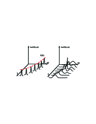
                  (a)                                            (b)

Figure 1: Evolution of the non-interacting spectrum (a) into the interacting spectrum (b) as the Coulomb interaction increases. Panels (a) and (b) correspond to LDA-like and DMFT-like solutions, respectively.

The development of methods for studying strongly–correlated materials has a long history in condensed matter physics. These efforts have traditionally focused on model Hamiltonians using techniques such as diagrammatic methods Bickers and Scalapino (1989), quantum Monte Carlo simulations Jarrell and Gubernatis (1996), exact diagonalization for finite–size clusters Dagotto (1994), density matrix renormalization group methods White (1992); U. Schollwöck (2005) and so on. Model Hamiltonians are usually written for a given solid–state system based on physical grounds. Development of LDA+U Anisimov et al. (1997b) and self–interaction corrected (SIC) Svane and Gunnarsson (1990); Szotek et al. (1993) methods, many–body perturbative approaches based on GW and its extensions Aryasetiawan and Gunnarsson (1998), as well as the time–dependent version of the density functional theory Gross et al. (1996) have been carried out by the electronic structure community. Some of these techniques are already much more complicated and time–consuming compared to the standard LDA based algorithms, and therefore the real exploration of materials is frequently performed by simplified versions utilizing approximations such as the plasmon–pole form for the dielectric function Hybertsen and Louie (1986), omitting the self–consistency within GW Aryasetiawan and Gunnarsson (1998) or assuming locality of the GW self–energy Zein and Antropov (2002).

The one–electron densities of states of strongly correlated systems may display both renormalized quasiparticles and atomic–like states simultaneously Georges and Kotliar (1992); Zhang et al. (1993). To treat them one needs a technique which is able to treat quasi-particle bands and Hubbard bands on the same footing, and which is able to interpolate between atomic and band limits. Dynamical mean–field theory Georges et al. (1996) is the simplest approach which captures these features; it has been extensively developed to study model Hamiltonians. Fig. 2 shows the development of the spectrum while increasing the strength of Coulomb interaction $U$ as obtained by DMFT solution of the Hubbard model. It illustrates the necessity to go beyond static mean–field treatments in the situations when the on–site Hubbard $U$ becomes comparable with the bandwidth $W$.

Figure 2: Local spectral density at $T=0$, for several values of $U$, obtained by the iterated perturbation theory approximation (from Zhang et al. (1993)).

Model Hamiltonian based DMFT methods have successfully described regimes $U/W\gtrsim 1$. However to describe strongly correlated materials we need to incorporate realistic electronic structure because the low–temperature physics of systems near localization–delocalization crossover is non–universal, system specific, and very sensitive to the lattice structure and orbital degeneracy which is unique to each compound. We believe that incorporating this information into the many–body treatment of this system is a necessary first step before more general lessons about strong–correlation phenomena can be drawn. In this respect, we recall that DFT in its common approximations, such as LDA or GGA, brings a system specific description into calculations. Despite the great success of DFT for studying weakly correlated solids, it has not been able thus far to address strongly–correlated phenomena. So, we see that both density functional based and many–body model Hamiltonian approaches are to a large extent complementary to each other. One–electron Hamiltonians, which are necessarily generated within density functional approaches (i.e. the hopping terms), can be used as input for more challenging many–body calculations. This path has been undertaken in a first paper of Anisimov et al. Anisimov et al. (1997a) which introduced the LDA+DMFT method of electronic structure for strongly–correlated systems and applied it to the photoemission spectrum of La_1-xSr_xTiO₃. Near the Mott transition, this system shows a number of features incompatible with the one–electron description Fujimori et al. (1992a). The electronic structure of Fe has been shown to be in better agreement with experiment within DMFT in comparison with LDA Lichtenstein and Katsnelson (1997, 1998). The photoemission spectrum near the Mott transition in V₂O₃ has been studied Held et al. (2001a), as well as issues connected to the finite temperature magnetism of Fe and Ni were explored Lichtenstein et al. (2001).

Despite these successful developments, we also would like to emphasize a more ambitious goal: to build a general method which treats all bands and all electrons on the same footing, determines both hoppings and interactions internally using a fully self–consistent procedure, and accesses both energetics and spectra of correlated materials. These efforts have been undertaken in a series of papers Chitra and Kotliar (2000a, 2001) which gave us a functional description of the problem in complete analogy to the density functional theory, and its self–consistent implementation is illustrated on Plutonium Savrasov et al. (2001); Savrasov and Kotliar (2004a).

To summarize, we see the existence of two roads in approaching the problem of simulating correlated materials properties, which we illustrate in Fig. 52. To describe these efforts in a language understandable by both electronic structure and many–body communities, and to stress qualitative differences and great similarities between DMFT and LDA, we start our review with discussing a general many–body framework based on the effective action approach to strongly–correlated systems Chitra and Kotliar (2001).

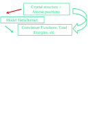
Figure 3: Two roads in approaching the problem of simulating correlated materials properties.

I.2 The effective action formalism and the constraining field

The effective action formalism, which utilizes functional Legendre transformations and the inversion method (for a comprehensive review see Fukuda et al. (1995), also see online notes), allows us to present a unified description of many seemingly different approaches to electronic structure. The idea is very simple, and has been used in other areas such as quantum field theory and statistical mechanics of spin systems. We begin with the free energy of the system written as a functional integral

$$\exp(-F)=\int D[\psi^{\dagger}\psi]e^{-S}.$$ (1)

where $F$ is the free energy, $S$ is the action for a given Hamiltonian, and $\psi$ is a Grassmann variable Negele and Orland (1998). One then selects an observable quantity of interest $A$, and couples a source $J$ to the observable $A$. This results in a modified action $S+JA$, and the free energy $F[J]$ is now a functional of the source $J$. A Legendre transformation is then used to eliminate the source in favor of the observable yielding a new functional

$$\Gamma[A]=F[J[A]]-{A}J[A]$$ (2)

$\Gamma[A]$ is useful in that the variational derivative with respect to $A$ yields $J$. We are free to set the source to zero, and thus the the extremum of $\Gamma[A]$ gives the free energy of the system.

The value of the approach is that useful approximations to the functional $\Gamma[A]$ can be constructed in practice using the inversion method, a powerful technique introduced to derive the TAP (Thouless, Anderson and Palmer) equations in spin glasses by Plefka (1982) and by  Fukuda (1988) to investigate chiral symmetry breaking in QCD (see also Refs. Georges and Yedidia (1991b); Opper and Winther (2001); Yedidia (2001); Fukuda et al. (1994)). The approach consists in carrying out a systematic expansion of the functional $\Gamma[A]$ to some order in a parameter or coupling constant $\lambda$. The action is written as $S=S_{0}+\lambda S_{1}$ and a systematic expansion is carried out

$$\Gamma[A]=\Gamma_{0}[A]+\lambda\Gamma_{1}[A]+...\ ,$$ (3)

$$J[A]=J_{0}[A]+\lambda J_{1}[A]+...\ .$$ (4)

A central point is that the system described by $S_{0}+AJ_{0}$ serves as a reference system for the fully interacting problem. It is a simpler system which by construction, reproduces the correct value of the observable $\widehat{A}$, and when this observable is properly chosen, other observables of the system can be obtained perturbatively from their values in the reference system. Hence $S_{0}+AJ_{0}$ is a simpler system which allows us to think perturbatively about the physics of a more complex problem. $J_{0}[A]$ is a central quantity in this formalism and we refer to it as the “constraining field”. It is the source that needs to be added to a reference action $S_{0}$ in order to produce a given value of the observable $A$.

It is useful to split the functional in this way

$$\Gamma[A]=\Gamma_{0}[A]+\Delta\Gamma[A]$$ (5)

since $\Gamma_{0}[A]=F_{0}[J_{0}]-AJ_{0}$ we could regard

$$\Gamma[A,J_{0}]={F_{0}}[J_{0}]-AJ_{0}+\Delta\Gamma[A]$$ (6)

as a functional which is stationary in two variables, the constraining field $J_{0}$ and A. The equation $\frac{\delta\Delta\Gamma}{\delta A}=J_{0}[A],$ together with the definition of $J_{0}[A]$ determines the exact constraining field for the problem.

One can also use the stationarity condition of the functional (6) to express A as a functional of $J_{0}$ and obtain a functional of the constraining field alone (ie. $\Gamma[J_{0}]=\Gamma[A[J_{0}],J_{0}]$). In the context of the Mott transition problem, this approach allowed a clear understanding of the analytical properties of the free energy underlying the dynamical mean field theory Kotliar (1999a).

$\Delta\Gamma$ can be a given a coupling constant integration representation which is very useful, and will appear in many guises through this review.

$$\Delta\Gamma[A]=\int_{0}^{1}d\lambda\frac{\partial\Gamma}{\partial\lambda}=\int_{0}^{1}d\lambda\langle S_{1}\rangle_{J(\lambda),\lambda}$$ (7)

Finally it is useful in many cases to decompose $\Delta\Gamma=E_{H}+\Phi_{xc},$ by isolating the Hartree contribution which can usually be evaluated explicitly. The success of the method relies on obtaining good approximations to the “generalized exchange correlation” functional $\Phi_{xc}.$

In the context of spin glasses, the parameter $\lambda$ is the inverse temperature and this approach leads very naturally to the TAP free energy. In the context of density functional theory, $\lambda$ is the strength of the electron–electron interactions as parameterized by the charge of the electron, and it can be used to present a very transparent derivation of the density functional approach Argaman and Makov (2000); Valiev and Fernando (1997); Fukuda et al. (1994); Chitra and Kotliar (2000a); Georges (2002); Savrasov and Kotliar (2004b). The central point is that the choice of observable, and the choice of reference system (i.e. the choice of $S_{0}$ which determines $J_{0}$) determine the structure of the (static or dynamic ) mean field theory to be used.

Notice that above we coupled a source linearly to the system of interest for the purpose of carrying out a Legendre transformation. It should be noted that one is free to add terms which contain powers higher than one in the source in order to modify the stability conditions of the functional without changing the properties of the saddle points. This freedom has been used to obtain functionals with better stability properties Chitra and Kotliar (2001).

We now illustrate these abstract considerations on a very concrete example. To this end we consider the full many–body Hamiltonian describing electrons moving in the periodic ionic potential $V_{ext}(\mathbf{r})$ and interacting among themselves according to the Coulomb law: $v_{C}(\mathbf{r}-\mathbf{r}^{\prime})=e^{2}/|\mathbf{r}-\mathbf{r}^{\prime}|$. This is the formal starting point of our all–electron first–principles calculation. So, the “theory of everything” is summarized in the Hamiltonian

$$H=\sum_{\sigma}\int d\mathbf{r}\psi^{+}_{\sigma}(\mathbf{r})[-{\bigtriangledown^{2}}+V_{ext}(\mathbf{r})-\mu]\psi_{\sigma}(\mathbf{r})$$ (8)

$$+{\frac{{1}}{2}}\sum_{\sigma\sigma^{\prime}}\int d\mathbf{r}d\mathbf{r}^{\prime}\psi_{\sigma}^{+}(\mathbf{r})\psi^{+}_{\sigma^{\prime}}(\mathbf{r}^{\prime})v_{C}(\mathbf{r}-\mathbf{r}^{\prime})\psi_{\sigma^{\prime}}(\mathbf{r}^{\prime})\psi_{\sigma}(\mathbf{r}).$$

Atomic Rydberg units, $\hbar=1,m_{e}=1/2$, are used throughout. Using the functional integral formulation in the imaginary time–frequency domain it is translated into the Euclidean action $S$

$$S=\int dx\psi^{+}(x)\partial_{\tau}\psi(x)+\int d\tau H(\tau),$$ (9)

where $x=(\mathbf{r}\tau\sigma)$. We will ignore relativistic effects in this action for simplicity. In addition the position of the atoms is taken to be fixed and we ignore the electron–phonon interaction. We refer the reader to several papers addressing that issue Freericks et al. (1993); Millis et al. (1996a).

The effective action functional approach Chitra and Kotliar (2001) allows one to obtain the free energy $F$ of a solid from a functional $\Gamma$ evaluated at its stationary point. The main question is the choice of the functional variable which is to be extremized. This question is highly non–trivial because the exact form of the functional is unknown and the usefulness of the approach depends on our ability to construct good approximations to it, which in turn depends on the choice of variables. At least two choices are very well–known in the literature: the exact Green’s function as a variable which gives rise to the Baym–Kadanoff (BK) theory Baym and Kadanoff (1961); Baym (1962) and the density as a variable which gives rise to the density functional theory. We review both approaches using an effective action point of view in order to highlight similarities and differences with the spectral density functional methods which will be presented on the same footing in Section II.

I.2.1 Density functional theory

Density functional theory in the Kohn–Sham formulation is one of the basic tools for studying weakly–interacting electronic systems and is widely used by the electronic structure community. We will review it using the effective action approach, which was introduced in this context by Fukuda Fukuda et al. (1994); Argaman and Makov (2000); Valiev and Fernando (1997).

$\bullet$ Choice of variables. The density of electrons $\rho(\mathbf{r})$ is the central quantity of DFT and it is used as a physical variable in derivation of DFT functional.

$\bullet$ Construction of exact functional. To construct the DFT functional we probe the system with a time–dependent source field $J(x)$. This modifies the action of the system (9) as follows

$$S^{\prime}[J]=S+\int dxJ(x)\psi^{+}(x)\psi(x).$$ (10)

The partition function $Z$ becomes a functional of the auxiliary source field $J$

$$Z[J]=\exp(-F[J])=\int D[\psi^{\dagger}\psi]e^{-S^{\prime}[J]}.$$ (11)

The effective action for the density, i.e., the density functional, is obtained as the Legendre transform of $F$ with respect to $\rho(x)$

$$\Gamma_{DFT}[\rho]=F[J]-\mathrm{Tr}\left(J\rho\right),$$ (12)

where trace $\mathrm{Tr}$ stands for

$$\mathrm{Tr}(J\rho)=\int dxJ(x)\rho(x)=T\sum_{i\omega}\int d\mathbf{r}J(\mathbf{r},i\omega)\rho(\mathbf{r},i\omega).$$ (13)

From this point forward, we shall restrict the source to be time independent because we will only be constructing the standard DFT. If the time dependence where retained, one could formulate time–dependent density functional theory (TDFT). The density appears as the variational derivative of the free energy with respect to the source

$$\rho(x)=\frac{\delta F}{\delta J(x)}.$$ (14)

$\bullet$ The constraining field in DFT. We shall demonstrate below that, in the context of DFT, the constraining field is the sum of the well known exchange–correlation potential and the Hartree potential $V_{xc}+V_{H}$, and we refer to this quantity as $V_{int}$. This is the potential which must be added to the non–interacting Hamiltonian in order to yield the exact density of the full Hamiltonian. Mathematically, $V_{int}$ is a functional of the density which solves the equation

$$\rho(\mathbf{r})=T\sum_{i\omega}\langle\mathbf{r}\left|[i\omega+\mu+\nabla^{2}-V_{ext}(\mathbf{r})-V_{int}(\mathbf{r})]^{-1}\right|\mathbf{r}\rangle e^{i\omega 0^{+}}.$$ (15)

The Kohn–Sham equation gives rise to a reference system of non–interacting particles, the so called Kohn–Sham orbitals $\psi_{\mathbf{k}j}$ which produce the interacting density

$$[-\nabla^{2}+V_{KS}(\mathbf{r})]\psi_{\mathbf{k}j}(\mathbf{r})=\epsilon_{\mathbf{k}j}\psi_{\mathbf{k}j}(\mathbf{r}),$$ (16)

$$\rho(\mathbf{r})=\sum_{\mathbf{k}j}f_{\mathbf{k}j}\psi_{\mathbf{k}j}^{\ast}(\mathbf{r})\psi_{\mathbf{k}j}(\mathbf{r}).$$ (17)

Here the Kohn–Sham potential is $V_{KS}=V_{ext}+V_{int}$, $\epsilon_{\mathbf{k}j},$ $\psi_{\mathbf{k}j}(\mathbf{r})$ are the Kohn–Sham energy bands and wave functions, $\mathbf{k}$ is a wave vector which runs over the first Brillouin zone, $j$ is band index, and $f_{\mathbf{k}j}=1/[\exp(\epsilon_{\mathbf{k}j}-\mu)/T+1]$ is the Fermi function.

$\bullet$ Kohn–Sham Green’s function. Alternatively, the electron density can be obtained with the help of the Kohn–Sham Green’s function, given by

$$G_{KS}^{-1}(\mathbf{r},\mathbf{r}^{\prime},i\omega)=G_{0}^{-1}(\mathbf{r},\mathbf{r}^{\prime},i\omega)-V_{int}(\mathbf{r})\delta(\mathbf{r}-\mathbf{r}^{\prime}),$$ (18)

where $G_{0}$ is the non–interacting Green’s function

$$G_{0}^{-1}(\mathbf{r},\mathbf{r}^{\prime},i\omega)=\delta(\mathbf{r}-\mathbf{r}^{\prime})[i\omega+\mu+\nabla^{2}-V_{ext}(\mathbf{r})],$$ (19)

and the density can then be computed from

$$\rho(\mathbf{r})=T\sum_{i\omega}G_{KS}(\mathbf{r},\mathbf{r},i\omega)e^{i\omega 0+}.$$ (20)

The Kohn–Sham Green’s function is defined in the entire space, where $V_{int}(\mathbf{r})$ is adjusted in such a way that the density of the system $\rho(\mathbf{r})$ can be found from $G_{KS}(\mathbf{r},\mathbf{r}^{\prime},i\omega)$. It can also be expressed in terms of the Kohn–Sham particles in the following way

$$G_{KS}(\mathbf{r},\mathbf{r}^{\prime},i\omega)=\sum_{\mathbf{k}j}\frac{\psi_{\mathbf{k}j}(\mathbf{r})\psi_{\mathbf{k}j}^{\ast}(\mathbf{r}^{\prime})}{i\omega+\mu-\epsilon_{\mathbf{k}j}}.$$ (21)

$\bullet$ Kohn–Sham decomposition. Now we come to the problem of writing exact and approximate expressions for the functional. The strategy consists in performing an expansion of the functional in powers of electron charge Chitra and Kotliar (2001); Fukuda et al. (1994); Valiev and Fernando (1997); Plefka (1982); Georges and Yedidia (1991a); Georges (2002). The Kohn–Sham decomposition consists of splitting the functional into the zeroth order term and the remainder.

$$\Gamma_{DFT}(\rho)=\Gamma_{DFT}(\rho,e^{2}=0)+\Delta\Gamma_{DFT}(\rho).$$ (22)

This is equivalent to what Kohn and Sham did in their original work. In the first term, $e^{2}=0$ only for the electron–electron interactions, and not for the interaction of the electron and the external potential. The first term consists of the kinetic energy of the Kohn–Sham particles and the external potential. The constraining field $J_{0}$ (see Eq. (4)) is $V_{int}$ since it generates the term that needs to be added to the non–interacting action in order to get the exact density. Furthermore, functional integration of the Eq. (11) gives $F[V_{int}]=-\mathrm{Tr}\ln[G_{0}^{-1}-V_{int}]$ Negele and Orland (1998) and from Eq. (12) it follows that

$$\Gamma_{DFT}(\rho,e^{2}=0)\equiv K_{DFT}[G_{KS}]=$$ (23)

$$-\mathrm{Tr}\ln(G_{0}^{-1}-V_{int}[G_{KS}])-\mathrm{Tr}\left(V_{int}[G_{KS}]G_{KS}\right).$$

The remaining part $\Delta\Gamma_{DFT}(\rho)$ is the interaction energy functional which is decomposed into the Hartree and exchange–correlation energies in a standard way

$$\Delta\Gamma_{DFT}(\rho)=E_{H}[\rho]+\Phi_{DFT}^{xc}[\rho].$$ (24)

${{\Phi^{xc}}_{DFT}}[\rho]$ at zero temperature becomes the standard exchange correlation energy in DFT, $E_{xc}[\rho]$.

$\bullet$ Kohn–Sham equations as saddle–point equations. The density functional $\Gamma_{DFT}(\rho)$ can be regarded as a functional which is stationary in two variables $V_{int}$ and $\rho$. Extremization with respect to $V_{int}$ leads to Eq. (18), while stationarity with respect to $\rho$ gives $V_{int}=\delta\Delta\Gamma/\delta\rho$, or equivalently,

$$V_{KS}[\rho](\mathbf{r}) =V_{ext}(\mathbf{r})+V_{int}[\rho](\mathbf{r})$$

$$=V_{ext}(\mathbf{r})+V_{H}[\rho](\mathbf{r})+V_{xc}[\rho](\mathbf{r}),$$ (25)

where $V_{xc}(\mathbf{r})$ is the exchange–correlation potential given by

$$V_{xc}(\mathbf{r})\equiv\frac{\delta\Phi_{DFT}^{xc}}{\delta\rho(\mathbf{r})}.$$ (26)

Equations (25) and (26) along with Eqs. (20) and (18) or, equivalently, (16) and (17) form the system of equations of the density functional theory. It should be noted that the Kohn-Sham equations give the true minimum of $\Gamma_{DFT}(\rho)$, and not only the saddle point.

$\bullet$ Exact representation for $\Phi_{DFT}^{xc}.$ The explicit form of the interaction functional $\Phi_{DFT}^{xc}[\rho]$ is not available. However, it may be defined by a power series expansion which can be constructed order by order using the inversion method. The latter can be given, albeit complicated, a diagrammatic interpretation. Alternatively, an expression for it involving integration by a coupling constant $\lambda e^{2}$ can be obtained using the Harris–Jones formula Harris and Jones (1974); Gunnarsson and Lundqvist (1976); Langreth and Perdew (1977); Georges (2002). One considers $\Gamma_{DFT}[\rho,\lambda]$ at an arbitrary interaction $\lambda$ and expresses it as

$$\Gamma_{DFT}[\rho,e^{2}]=\Gamma_{DFT}[\rho,0]+\int_{0}^{1}d\lambda\frac{\partial\Gamma_{DFT}[\rho,\lambda]}{\partial\lambda}.$$ (27)

Here the first term is simply $K_{DFT}[G_{KS}\mathcal{]}$ as given by (23) which does not depend on $\lambda$. The second part is thus the unknown functional $\Phi_{DFT}^{xc}[\rho].$ The derivative with respect to the coupling constant in (27) is given by the average $\langle\psi^{+}(x)\psi^{+}(x^{\prime})\psi(x^{\prime})\psi(x)\rangle=\Pi_{\lambda}(x,x^{\prime},i\omega)+$ $\langle\psi^{+}(x)\psi(x)\rangle\langle\psi^{+}(x^{\prime})\psi(x^{\prime})\rangle$ where $\Pi_{\lambda}(x,x^{\prime})$ is the density–density correlation function at a given interaction strength $\lambda$ computed in the presence of a source which is $\lambda$ dependent  and chosen so that the density of the system was $\rho$. Since $\langle\psi^{+}(x)\psi(x)\rangle=\rho(x),$ one can obtain

$$\Phi_{DFT}[\rho]=E_{H}[\rho]+\sum_{i\omega}\int d^{3}\mathbf{r}d^{3}\mathbf{r}^{\prime}\int_{0}^{1}d\lambda\frac{\Pi_{\lambda}(\mathbf{r},\mathbf{r}^{\prime},i\omega)}{|\mathbf{r}-\mathbf{r}^{\prime}|}.$$ (28)

This expression has been used to construct more accurate exchange correlation functionals Dobson et al. (1997).

$\bullet$ Approximations. Since $\Phi_{DFT}^{xc}[\rho]$ is not known explicitly some approximations are needed. The LDA assumes

$$\Phi_{DFT}^{xc}[\rho]=\int\rho(\mathbf{r})\epsilon_{xc}[\rho(\mathbf{r})]d\mathbf{r},$$ (29)

where $\epsilon_{xc}[\rho(\mathbf{r})]$ is the exchange–correlation energy of the uniform electron gas, which is easily parameterized. $V_{eff}$ is given as an explicit function of the local density. In practice one frequently uses the analytical formulae von Barth and Hedin (1972); Gunnarsson et al. (1976); Moruzzi et al. (1978); Vosko et al. (1980); Perdew and Yue (1992). The idea here is to fit a functional form to quantum Monte Carlo (QMC) calculations Ceperley and Alder (1980). Gradient corrections to the LDA have been worked out by Perdew and coworkers Perdew et al. (1996). They are also frequently used in LDA calculations.

$\bullet$ Evaluation of the total energy. At the saddle point, the density functional $\Gamma_{DFT}$ delivers the total free energy of the system

$$F=\mathrm{Tr}\ln G_{KS}-\mathrm{Tr}\left(V_{int}\rho\right)+E_{H}[\rho]+\Phi_{DFT}^{xc}[\rho],$$ (30)

where the trace in the second term runs only over spatial coordinates and not over imaginary time. If temperature goes to zero, the entropy contribution vanishes and the total energy formulae is recovered

$$E=-\mathrm{Tr}(\nabla^{2}G_{KS})+\mathrm{Tr}\left(V_{ext}\rho\right)+E_{H}[\rho]+E_{DFT}^{xc}[\rho].$$ (31)

$\bullet$ Assessment of the approach. From a conceptual point of view, the density functional approach is radically different from the Green’s function theory (See below). The Kohn–Sham equations (16), (17) describe the Kohn–Sham quasiparticles which are poles of $G_{KS}$ and are not rigorously identifiable with one–electron excitations. This is very different from the Dyson equation (see below Eq. (41)) which determines the Green’s function $G$, which has poles at the observable one–electron excitations. In principle the Kohn–Sham orbitals are a technical tool for generating the total energy as they alleviate the kinetic energy problem. They are however not a necessary element of the approach as DFT can be formulated without introducing the Kohn-Sham orbitals. In practice, they are also used as a first step in perturbative calculations of the one–electron Green’s function in powers of screened Coulomb interaction, as e.g. the GW method. Both the LDA and GW methods are very successful in many materials for which the standard model of solids works. However, in correlated electron system this is not always the case. Our view is that this situation cannot be remedied by either using more complicated exchange– correlation functionals in density functional theory or adding a finite number of diagrams in perturbation theory. As discussed above, the spectra of strongly–correlated electron systems have both correlated quasiparticle bands and Hubbard bands which have no analog in one–electron theory.

The density functional theory can also be formulated for the model Hamiltonians, the concept of density being replaced by the diagonal part of the density matrix in a site representation. It was tested in the context of the Hubbard model by Hess and Serene (1999); Lima et al. (2002); Schonhammer et al. (1995).

I.2.2 Baym–Kadanoff functional

The Baym–Kadanoff functional Baym and Kadanoff (1961); Baym (1962) gives the one–particle Green’s function and the total free energy at its stationary point. It has been derived in many papers starting from deDominicis and Martin (1964a, b) and Cornwall et al. (1974) (see also Chitra and Kotliar (2000a, 2001); Georges (2004a, b)) using the effective action formalism.

$\bullet$ Choice of variable.  The one–electron Green’s function $G(x,x^{\prime})=-\langle T_{\tau}\psi(x)\psi^{+}(x^{\prime})\rangle$, whose poles determine the exact spectrum of one–electron excitations, is at the center of interest in this method and it is chosen to be the functional variable.

$\bullet$ Construction of exact functional. As it has been emphasized Chitra and Kotliar (2001), the Baym–Kadanoff functional can be obtained by the Legendre transform of the action. The electronic Green’s function of a system can be obtained by probing the system by a source field and monitoring the response. To obtain $\Gamma_{BK}[G]$ we probe the system with a time–dependent two–variable source field $J(x,x^{\prime})$. Introduction of the source $J(x,x^{\prime})$ modifies the action of the system (9) in the following way

$$S^{\prime}[J]=S+\int dxdx^{\prime}J(x,x^{\prime})\psi^{+}(x)\psi(x^{\prime}).$$ (32)

The average of the operator $\psi^{+}(x)\psi(x^{\prime})$ probes the Green’s function. The partition function $Z,$ or equivalently the free energy of the system $F,$ becomes a functional of the auxiliary source field

$$Z[J]=\exp(-F[J])=\int D[\psi^{+}\psi]e^{-S^{\prime}[J]}.$$ (33)

The effective action for the Green’s function, i.e., the Baym–Kadanoff functional, is obtained as the Legendre transform of $F$ with respect to $G(x,x^{\prime})$

$$\Gamma_{BK}[G]=F[J]-\mathrm{Tr}(JG),$$ (34)

where we use the compact notation $\mathrm{Tr}(JG)$ for the integrals

$$\mathrm{Tr}(JG)=\int dxdx^{\prime}J(x,x^{\prime})G(x^{\prime},x).$$ (35)

Using the condition

$$G(x,x^{\prime})=\frac{\delta F}{\delta J(x^{{}^{\prime}},x)},$$ (36)

to eliminate $J$ in (34) in favor of the Green’s function, we finally obtain the functional of the Green’s function alone.

$\bullet$ Constraining field in the Baym–Kadanoff theory. In the context of the Baym–Kadanoff approach, the constraining field is the familiar electron self–energy $\Sigma_{int}(\mathbf{r},\mathbf{r}^{\prime},i\omega)$. This is the function which needs to be added to the inverse of the non–interacting Green’s function to produce the inverse of the exact Green’s function, i.e.,

$$G^{-1}(\mathbf{r},\mathbf{r}^{\prime},i\omega)=G_{0}^{-1}(\mathbf{r},\mathbf{r}^{\prime},i\omega)-\Sigma_{int}(\mathbf{r},\mathbf{r}^{\prime},i\omega).$$ (37)

Here $G_{0}$ is the non–interacting Green’s function given by Eq. (19). Also, if the Hartree potential is written explicitly, the self–energy can be split into the Hartree, $V_{H}(\mathbf{r})=\int v_{C}(\mathbf{r}-\mathbf{r}^{\prime})\rho(\mathbf{r}^{\prime})d\mathbf{r}^{\prime}$ and the exchange–correlation part, $\Sigma_{xc}(\mathbf{r},\mathbf{r}^{\prime},i\omega).$

Ultimately, having fixed $G_{0}$ the self–energy becomes a functional of $G$, i.e. $\Sigma_{int}[G].$

$\bullet$ Kohn–Sham decomposition. We now come to the problem of writing various contributions to the Baym–Kadanoff functional. This development parallels exactly what was done in the DFT case. The strategy consists of performing an expansion of the functional $\Gamma_{BK}[G]$ in powers of the charge of electron entering the Coulomb interaction term at fixed $G$ Chitra and Kotliar (2001); Fukuda et al. (1994); Valiev and Fernando (1997); Plefka (1982); Georges and Yedidia (1991a); Georges (2002, 2004a, 2004b). The zeroth order term is denoted $K$, and the sum of the remaining terms $\Phi$, i.e.

$$\Gamma_{BK}[G]=K_{BK}[G]+\Phi_{BK}[G].$$ (38)

$K$ is the kinetic part of the action plus the energy associated with the external potential $V_{ext}$. In the Baym–Kadanoff theory this term has the form

$$K_{BK}[G] = \Gamma_{BK}[G,e^{2}=0]=$$

$$- \mathrm{Tr}\ln(G_{0}^{-1}-\Sigma_{int}[G])-\mathrm{Tr}\left(\Sigma_{int}[G]G\right).$$

$\bullet$ Saddle–point equations. The functional (38) can again be regarded as a functional stationary in two variables, $G$ and constraining field $J_{0}$, which is $\Sigma_{int}$ in this case. Extremizing with respect to $\Sigma_{int}$ leads to the Eq. (37), while extremizing with respect to $G$ gives the definition of the interaction part of the electron self–energy

$$\Sigma_{int}(\mathbf{r},\mathbf{r}^{\prime},i\omega)=\frac{\delta\Phi_{BK}[G]}{\delta G(\mathbf{r}^{\prime},\mathbf{r},i\omega)}.$$ (40)

Using the definition for $G_{0}$ in Eq. (19), the Dyson equation (37) can be written in the following way

$$[\nabla^{2}-V_{ext}(\mathbf{r})+i\omega+\mu]G(\mathbf{r},\mathbf{r}^{\prime},i\omega) -$$ (41)

$$\int d\mathbf{r}^{\prime\prime}\Sigma_{int}(\mathbf{\ r},\mathbf{r}^{\prime\prime},i\omega)G(\mathbf{r}^{\prime\prime},\mathbf{r}^{\prime},i\omega) = \delta(\mathbf{r}-\mathbf{r}^{\prime}).$$

The Eqs. (40) and (41) constitute a system of equations for $G$ in the Baym–Kadanoff theory.

$\bullet$ Exact representation for $\Phi.$ Unfortunately, the interaction energy functional $\Phi_{BK}[G]$ is unknown. One can prove that it can be represented as a sum of all two–particle irreducible diagrams constructed from the Green’s function $G$ and the bare Coulomb interaction. In practice, we almost always can separate the Hartree diagram from the remaining part the so called exchange–correlation contribution

$$\Phi_{BK}[G]=E_{H}[\rho]+\Phi_{BK}^{xc}[G].$$ (42)

$\bullet$ Evaluation of the total energy. At the stationarity point, $\Gamma_{BK}[G]$ delivers the free energy $F$ of the system

$$F=\mathrm{Tr}\ln G-\mathrm{Tr}\left(\Sigma_{int}G\right)+E_{H}[\rho]+\Phi_{BK}^{xc}[G],$$ (43)

where the first two terms are interpreted as the kinetic energy and the energy related to the external potential, while the last two terms correspond to the interaction part of the free energy. If temperature goes to zero, the entropy part vanishes and the total energy formula is recovered

$$E_{tot}=-\mathrm{Tr}(\nabla^{2}G)+\mathrm{Tr}(V_{ext}G)+E_{H}[\rho]+E_{BK}^{xc}[G],$$ (44)

where $E_{BK}^{xc}=1/2\mathrm{Tr}\left(\Sigma_{xc}G\right)$ Fetter and Walecka (1971) (See also online notes).

$\bullet$ Functional of the constraining field, self-energy functional approach. Expressing the functional in Eq. (38) in terms of the constraining field, (in this case $\Sigma$ rather than the observable $G$) recovers the self-energy functional approach proposed by Potthoff Potthoff (2003b, a, 2005).

$$\Gamma[\Sigma]=-\mathrm{Tr}\ln[{G_{0}}^{-1}-\Sigma]+Y[\Sigma]$$ (45)

$Y[\Sigma]$ is the Legendre transform with respect to $G$ of the Baym Kadanoff functional $\Phi_{BK}[G]$. While explicit representations of the Baym Kadanoff functional $\Phi$ are available for example as a sum of skeleton graphs, no equivalent expressions have yet been obtained for $Y[\Sigma]$.

$\bullet$ Assessment of approach. The main advantage of the Baym–Kadanoff approach is that it delivers the full spectrum of one–electron excitations in addition to the ground state properties. Unfortunately, the summation of all diagrams cannot be performed explicitly and one has to resort to partial sets of diagrams, such as the famous GW approximation Hedin (1965) which has only been useful in the weak–coupling situations.Resummation of diagrams to infinite order guided by the concept of locality, which is the basis of the Dynamical Mean Field Approximation, can be formulated neatly as truncations of the Baym Kadanoff functional as will be shown in the following sections.

I.2.3 Formulation in terms of the screened interaction

It is sometimes useful to think of Coulomb interaction as a screened interaction mediated by a Bose field. This allows one to define different types of approximations. In this context, using the locality approximation for irreducible quantities gives rise to the so–called Extended–DMFT, as opposed to the usual DMFT. Alternatively, the lowest order Hartree–Fock approximation in this formulation leads to the famous GW approximation.

An independent variable of the functional is the dynamically screened Coulomb interaction $W(\mathbf{r},\mathbf{r}^{\prime},i\omega)$ Almbladh et al. (1999) see also Chitra and Kotliar (2001). In the Baym–Kadanoff theory, this is done by introducing an auxiliary Bose variable coupled to the density, which transforms the original problem into a problem of electrons interacting with the Bose field. The screened interaction $W$ is the connected correlation function of the Bose field.

By applying the Hubbard–Stratonovich transformation to the action in Eq. (9) to decouple the quartic Coulomb interaction, one arrives at the following action

$$S=\int dx\psi^{+}(x)\Bigl{(}\partial_{\tau}-\mu-{\bigtriangledown^{2}}+V_{ext}(x)+V_{H}(x)\Bigr{)}\psi(x)$$

$$+{\frac{{1}}{2}}\int dxdx^{\prime}\phi(x)v_{C}^{-1}(x-x^{\prime})\phi(x^{\prime})$$

$$-ig\int dx\phi(x)\Bigl{(}\psi^{+}(x)\psi(x)-\langle\psi^{+}(x)\psi(x)\rangle_{S}\Bigr{)}$$ (46)

where $\phi(x)$ is a Hubbard–Stratonovich field, $V_{H}(x)$ is the Hartree potential, $g$ is a coupling constant to be set equal to one at the end of the calculation and the brackets denote the average with the action $S$. In Eq. (46), we omitted the Hartree Coulomb energy which appears as an additive constant, but it will be restored in the full free energy functional. The Bose field, in this formulation has no expectation value (since it couples to the “normal order” term).

$\bullet$ Baym–Kadanoff functional of $G$ and $W$. Now we have a system of interacting fermionic and bosonic fields. By introducing two source fields $J$ and $K$ we probe the electron Green’s function $G$ defined earlier and the boson Green’s function $W=\langle T_{\tau}\phi(x)\phi(x^{\prime})\rangle$ to be identified with the screened Coulomb interaction. The functional is thus constructed by supplementing the action Eq. (46) by the following term

$$S^{\prime}[J,K]=S + \int dxdx^{\prime}J(x,x^{\prime})\psi^{\dagger}(x)\psi(x^{\prime})$$ (47)

$$+ \int dxdx^{\prime}K(x,x^{\prime})\phi(x)\phi(x^{\prime}).$$

The normal ordering of the interaction ensures that $\langle\phi(x)\rangle=0$. The constraining fields, which appear as the zeroth order terms in expanding $J$ and $K$ (see Eq. (4)), are denoted by $\Sigma_{int}$ and $\Pi$, respectively. The zeroth order free energy is then

$$F_{0}[\Sigma_{int},\Pi]=-\mathrm{Tr}\left(G_{0}^{-1}-\Sigma_{int}\right)+\frac{1}{2}\mathrm{Tr}\left(v_{C}^{-1}-\Pi\right),$$ (48)

therefore the Baym–Kadanoff functional becomes

$$\Gamma_{BK}[G,W]=-\mathrm{Tr}\ln\left(G_{0}^{-1}-\Sigma_{int}\right)-\mathrm{Tr}\left(\Sigma_{int}G\right)$$ (49)

$$+\frac{1}{2}\mathrm{Tr}\ln\left(v_{C}^{-1}-\Pi\right)+\frac{1}{2}\mathrm{Tr}\left(\Pi\,W\right)+\Phi_{BK}[G,W].$$

Again, $\Phi_{BK}[G,W]$ can be split into Hartree contribution and the rest

$$\Phi_{BK}[G,W]=E_{H}[\rho]+\Psi_{BK}[G,W].$$ (50)

The entire theory is viewed as the functional of both $G$ and $W.$ One of the strengths of such formulation is that there is a very simple diagrammatic interpretation for $\Psi_{BK}[G,W]$. It is given as the sum of all two–particle irreducible diagrams constructed from $G$ and $W$ Cornwall et al. (1974) with the exclusion of the Hartree term. The latter $E_{H}[\rho]$, is evaluated with the bare Coulomb interaction.

$\bullet$ Saddle point equations. Stationarity with respect to $G$ and $\Sigma_{int}$ gives rise to Eqs. (40) and (37), respectively. An additional stationarity condition $\delta\Gamma_{BK}/\delta W=0$ leads to equation for the screened Coulomb interaction $W$

$$W^{-1}(\mathbf{r},\mathbf{r}^{\prime},i\omega)=v_{C}^{-1}(\mathbf{r}-\mathbf{r}^{\prime})-\Pi(\mathbf{r},\mathbf{r}^{\prime},i\omega),$$ (51)

where function $\Pi(\mathbf{r},\mathbf{r}^{\prime},i\omega)=-2\delta\Psi_{BK}/\delta W(\mathbf{r}^{\prime},\mathbf{r},i\omega)$ is the susceptibility of the interacting system.

I.2.4 Approximations

The functional formulation in terms of a “screened” interaction $W$ allows one to formulate numerous approximations to the many–body problem. The simplest approximation consists in keeping the lowest order Hartree–Fock graph in the functional $\Psi_{BK}[G,W]$. This is the celebrated GW approximation Hedin (1965); Hedin and Lundquist (1969) (see Fig. 4). To treat strong correlations one has to introduce dynamical mean field ideas, which amount to a restriction of the functionals $\Phi_{BK},\Psi_{BK}$ to the local part of the Greens function (see section II). It is also natural to restrict the correlation function of the Bose field $W$, which corresponds to including information about the four point function of the Fermion field in the self-consistency condition, and goes under the name of the Extended Dynamical Mean–Field Theory (EDMFT) Bray and Moore (1980); Sachdev and Ye (1993); Sengupta and Georges (1995); Kajueter (1996a); Kajueter and Kotliar (1996a); Si and Smith (1996); Smith and Si (2000); Chitra and Kotliar (2001).

This methodology has been useful in incorporating effects of the long range Coulomb interactions  Chitra and Kotliar (2000b) as well as in the study of heavy fermion quantum critical points, Si et al. (2001); Si et. al. et al. (1999) and quantum spin glasses  Bray and Moore (1980); Sengupta and Georges (1995); Sachdev and Ye (1993)

More explicitly, in order to zero the off–diagonal Green’s functions (see Eq. (54)) we introduce a set of localized orbitals $\Phi_{R\alpha}(r)$ and express $G$ and $W$ through an expansion in those orbitals.

$$G(r,r^{\prime},i\omega)=\sum_{RR^{\prime}\alpha\beta}G_{R\alpha,R^{\prime}\beta}(i\omega)\Phi_{R\alpha}^{*}(r)\Phi_{R^{\prime}\beta}(r^{\prime}),$$ (52)

$$W(r,r^{\prime},i\omega)=\sum_{R_{1}\alpha,R_{2}\beta,R_{3}\gamma,R_{4}\delta}W_{R_{1}\alpha,R_{2}\beta,R_{3}\gamma,R_{4}\delta}(i\omega)\times\\ \Phi^{*}_{R_{1}\alpha}(r)\Phi^{*}_{R_{2}\beta}(r^{\prime})\Phi_{R_{3}\gamma}(r^{\prime})\Phi_{R_{4}\delta}(r).$$ (53)

The approximate EDMFT functional is obtained by restriction of the correlation part of the Baym–Kadanoff functional $\Psi_{BK}$ to the diagonal parts of the $G$ and $W$ matrices:

$$\Psi_{EDMFT}=\Psi_{BK}[G_{RR},W_{RRRR}]$$ (54)

The EDMFT graphs are shown in Fig. 4.

Figure 4: The Baym–Kadanoff functional $\Phi$ for various approximations for electron–boson action Eq. (46). In all cases, the bare Hartree diagrams have been omitted. The first line shows the famous GW approximation where only the lowest order Hartree and Fock skeleton diagrams are kept. The second line corresponds to Extended–Dynamical Mean–Field Theory that sums up all the local graphs. Three dots represent all the remaining skeleton graphs which include local $G$ and local $W$ only. The combination of GW and EDMFT is straightforward. All lowest order Fock graphs are included (local and nonlocal). The higher order graphs are restricted to one site only (adapted from Sun and Kotliar (2002, 2004)).

It is straightforward to combine the GW and EDMFT approximations by keeping the nonlocal part of the exchange graphs as well as the local parts of the correlation graphs (see Fig. 4).

The GW approximation derived from the Baym–Kadanoff functional is a fully self–consistent approximation which involves all electrons. In practice sometimes two approximations are used: a) in pseudopotential treatments only the self–energy of the valence and conduction electrons are considered and b) instead of evaluating $\Pi$ and $\Sigma$ self–consistently with $G$ and $W$, one does a “one–shot” or one iteration approximation where $\Sigma$ and $\Pi$ are evaluated with $G_{0}$, the bare Green’s function which is sometimes taken as the LDA Kohn–Sham Green’s function, i.e., $\Sigma\approx\Sigma[G_{0},W_{0}]$ and $\Pi=\Pi[G_{0}]$. The validity of these approximations and importance of the self–consistency for the spectra evaluation was explored in Wei Ku (2002); Holm and von Barth (1998); Arnaud and Alouani (2000); Hybertsen and Louie (1985); Holm (1999); Tiago et al. (2003). The same issues arise in the context of GW+EDMFT  Sun and Kotliar (2004).

At this point, the GW+EDMFT has been fully implemented on the one–band model Hamiltonian level Sun and Kotliar (2004, 2002). A combination of GW and LDA+DMFT was applied to Nickel, where $W$ in the EDMFT graphs is approximated by the Hubbard $U$, in Refs. Biermann et al. (2003) and Biermann et al. (2004); Aryasetiawan et al. (2004a).

I.2.5 Model Hamiltonians and first principles approaches

In this section we connect the previous sections which were based on real $\mathbf{r}$-space with the notation to be used later in the review which use local basis sets. We perform a transformation to a more general basis set of possibly non–orthogonal orbitals $\chi_{\xi}(\mathbf{r})$ which can be used to represent all the relevant quantities in our calculation. As we wish to utilize sophisticated basis sets of modern electronic structure calculations, we will sometimes waive the orthogonality condition and introduce the overlap matrix

$$O_{\xi\xi^{\prime}}=\langle\chi_{\xi}|\chi_{\xi^{\prime}}\rangle.$$ (55)

The field operator $\psi(x)$ becomes

$$\psi(x)=\sum_{\xi}c_{\xi}(\tau)\chi_{\xi}(\mathbf{r}),$$ (56)

where the coefficients $c_{\xi}$ are new operators acting in the orbital space $\{\chi_{\xi}\}.$ The Green’s function is represented as

$$G(\mathbf{r},\mathbf{r}^{\prime},\tau)=\sum_{\xi\xi^{\prime}}\chi_{\xi}(\mathbf{r})G_{\xi\xi^{\prime}}(\tau)\chi_{\xi^{\prime}}^{\ast}(\mathbf{r}^{\prime}),$$ (57)

and the free energy functional $\Gamma_{BK}$ as well as the interaction energy $\Phi$ are now considered as functionals of the coefficients $G_{\xi\xi^{\prime}}$ either on the imaginary time axis, $G_{\xi\xi^{\prime}}(\tau)$ or imaginary frequency axis $G_{\xi\xi^{\prime}}(i\omega),$ which can be analytically continued to real times and energies.

In most cases we would like to interpret the orbital space $\{\chi_{\xi}\}$ as a general tight–binding basis set where the index $\xi$ combines the angular momentum index $lm$, and the unit cell index $\mathbf{R},$ i.e., $\chi_{\xi}(\mathbf{r})=\chi_{lm}(\mathbf{r}-\mathbf{R})=\chi_{\alpha}(\mathbf{r}-\mathbf{R}).$ Note that we can add additional degrees of freedom to the index $\alpha$ such as multiple kappa basis sets of the linear muffin–tin orbital based methods Andersen (1975); Andersen and Jepsen (1984); Methfessel (1988); Weyrich (1988); Blöechl (1989); Savrasov (1992, 1996). If more than one atom per unit cell is considered, index $\alpha$ should be supplemented by the atomic basis position within the unit cell, which is currently omitted for simplicity. For spin unrestricted calculations $\alpha$ accumulates the spin index $\sigma$ and the orbital space is extended to account for the eigenvectors of the Pauli matrix.

It is useful to write down the Hamiltonian containing the infinite space of the orbitals

$$\hat{H}=\sum_{\xi\xi^{\prime}}h_{\xi\xi^{\prime}}^{(0)}[c_{\xi}^{+}c_{\xi^{\prime}}+h.c.]+\frac{1}{2}\sum_{\xi\xi^{\prime}\xi^{\prime\prime}\xi^{\prime\prime\prime}}V_{\xi\xi^{\prime}\xi^{\prime\prime}\xi^{\prime\prime\prime}}c_{\xi}^{+}c_{\xi^{\prime}}^{+}c_{\xi^{\prime\prime}}c_{\xi^{\prime\prime\prime}},$$ (58)

where $h_{\xi\xi^{\prime}}^{(0)}=\langle\chi_{\xi}|-\nabla^{2}+V_{ext}|\chi_{\xi^{\prime}}\rangle$ is the non–interacting Hamiltonian and the interaction matrix element is $V_{\xi\xi^{\prime}\xi^{\prime\prime}\xi^{\prime\prime\prime}}=\langle\chi_{\xi}(r)\chi_{\xi^{\prime}}(r^{\prime})|v_{C}|\chi_{\xi^{\prime\prime}}(r^{\prime})\chi_{\xi^{\prime\prime\prime}}(r)\rangle.$ Using the tight–binding interpretation this Hamiltonian becomes

$$\hat{H}=\sum_{\alpha\beta}\sum_{RR^{\prime}}h_{\alpha R\beta R^{\prime}}^{(0)}\bigl{(}c_{\alpha R}^{+}c_{\beta R^{\prime}}+h.c.\bigr{)}\\ +\frac{1}{2}\sum_{\alpha\beta\gamma\delta}\sum_{RR^{\prime}R^{\prime\prime}R^{\prime\prime\prime}}V_{\alpha\beta\gamma\delta}^{RR^{\prime}R^{\prime\prime}R^{\prime\prime\prime}}c_{\alpha R}^{+}c_{\beta R^{\prime}}^{+}c_{\delta R^{\prime\prime\prime}}c_{\gamma R^{\prime\prime}},$$ (59)

where the diagonal elements $h_{\alpha R\beta R}^{(0)}\equiv h_{\alpha\beta}^{(0)}$ can be interpreted as the generalized atomic levels matrix $\epsilon_{\alpha\beta}^{(0)}$ (which does not depend on $R$ due to periodicity) and the off–diagonal elements $h_{\alpha R\beta R^{\prime}}^{(0)}(1-\delta_{RR^{\prime}})$ as the generalized hopping integrals matrix $t_{\alpha R\beta R^{\prime}}^{(0)}.$

I.2.6 Model Hamiltonians

Strongly correlated electron systems have been traditionally described using model Hamiltonians. These are simplified Hamiltonians which have the form of Eq. (59) but with a reduced number of band indices and sometimes assuming a restricted form of the Coulomb interaction which is taken to be very short ranged. The spirit of the approach is to describe a reduced number of degrees of freedom which are active in a restricted energy range to reduce the complexity of a problem and increase the accuracy of the treatment. Famous examples are the Hubbard model (one band and multiband) and the Anderson lattice model.

The form of the model Hamiltonian is often guessed on physical grounds and its parameters chosen to fit a set of experiments. In principle a more explicit construction can be carried out using tools such as screening canonical transformations first used by Bohm and Pines to eliminate the long range part of the Coulomb interaction  Bohm and Pines (1951, 1952, 1953), or a Wilsonian partial elimination (or integrating out) of the high–energy degrees of freedom Wilson (1975). However, these procedures are rarely used in practice.

One starts from an action describing a large number of degrees of freedom (site and orbital omitted)

$$S[{c}{{}^{+}}{c}]=\int d{x}\left({c}{{}^{+}}{O}\partial_{\tau}{c}+H[{c}{{}^{+}}{c}]\right),$$ (60)

where the orbital overlap $O_{\alpha R\beta R^{\prime}}$ appears and the Hamiltonian could have the form (59). Second, one divides the set of operators in the path integral in $c_{H}$ describing the “high–energy” orbitals which one would like to eliminate, and $c_{L}$ describing the low–energy orbitals that one would like to consider explicitly. The high–energy degrees of freedom are now integrated out. This operation defines the effective action for the low–energy variables Wilson (1983):

$$\frac{1}{Z_{eff}}\exp(-S_{eff}[{c}^{+}_{L}{c}_{L}]{)}=\frac{1}{Z}\int d{c}_{H}^{+}d{c}_{H}\exp(-S[c_{H}^{+}c_{L}^{+}c_{L}c_{H}]).$$ (61)

The transformation (61) generates retarded interactions of arbitrarily high order. If we focus on sufficiently low energies, frequency dependence of the coupling constants beyond linear order and non–linearities beyond quartic order can be neglected since they are irrelevant around a Fermi liquid fixed point Shankar (1994). The resulting physical problem can then be cast in the form of an effective model Hamiltonian. Notice however that when we wish to consider a broad energy range the full frequency dependence of the couplings has to be kept as demonstrated in an explicit approximate calculation using the GW method  Aryasetiawan et al. (2004b). The same ideas can be implemented using canonical transformations and examples of approximate implementation of this program are provided by the method of cell perturbation theory  Raimondi et al. (1996) and the generalized tight-binding method Ovchinnikov and Sandalov (1989).

The concepts and the rational underlying the model Hamiltonian approach are rigorous. There are very few studies of the form of the Hamiltonians obtained by screening and elimination of high–energy degrees of freedom, and the values of the parameters present in those Hamiltonians. Notice however that if a form for the model Hamiltonian is postulated, any technique which can be used to treat Hamiltonians approximately, can be also used to perform the elimination (61). A considerable amount of effort has been devoted to the evaluations of the screened Coulomb parameter $U$ for a given material. Note that this value is necessarily connected to the basis set representation which is used in deriving the model Hamiltonian. It should be thought as an effectively downfolded Hamiltonian to take into account the fact that only the interactions at a given energy interval are included in the description of the system. More generally, one needs to talk about frequency–dependent interaction $W$ which appears for example in the GW method. The outlined questions have been addressed in many previous works Dederichs et al. (1984); McMahan et al. (1988); Hybertsen et al. (1989); Springer and Aryasetiawan (1998); Kotani (2000). Probably, one of the most popular methods here is a constrained density functional approach formulated with general projection operators Dederichs et al. (1984); Meider and Springborg (1998). First, one defines the orbitals set which will be used to define correlated electrons. Second, the on–site density matrix defined for these orbitals is constrained by introducing additional constraining fields in the density functional. Evaluating second order derivative of the total energy with respect to the density matrix should in principle give us the access to $U$s. The problem is how one subtracts the kinetic energy part which appears in this formulation of the problem. Gunnarsson Gunnarsson (1990) and others  McMahan and Martin (1988); Freeman et al. (1987); Norman and Freeman (1986) have introduced a method which effectively cuts the hybridization of matrix elements between correlated and uncorrelated orbitals eliminating the kinetic contribution. This approach was used by McMahan et al. McMahan et al. (1988) in evaluating the Coulomb interaction parameters in the high–temperature superconductors. An alternative method has been used by Hybertsen et al. Hybertsen et al. (1989) who performed simultaneous simulations using the LDA and solution of the model Hamiltonian at the mean–field level. The total energy under the constraint of fixed occupancies was evaluated within both approaches. The value of $U$ is adjusted to make the two calculations coincide.

Much work has been done by the group of Anisimov who have performed evaluations of the Coulomb and exchange interactions for various systems such as NiO, MnO, CaCuO₂ and so on Anisimov et al. (1991). Interestingly, the values of $U$ deduced for such itinerant system as Fe can be as large as 6 eV Anisimov and Gunnarsson (1991). This highlights an important problem on deciding which electrons participate in the screening process. As a rule of thumb, one can argue that if we consider the entire $d$-shell as a correlated set, and allow its screening by $s$- and $p$-electrons, the values of $U$ appear to be between 5 and 10 eV on average. On the other hand, in many situations crystal field splitting between $t_{2g}$ and $e_{g}$ levels allows us to talk about a subset of a given crystal field symmetry (say, $t_{2g}$), and allowing screening by another subset (say by $e_{g}$). This usually leads to much smaller values of $U$ within range of 1-4 eV.

It is possible to extract the value of $U$ from GW calculations. The simplest way to define the parameter $U=W$ ($\omega=0$). There are also attempts to avoid the double counting inherent in that procedure Aryasetiawan et al. (2004b); Springer and Aryasetiawan (1998); Kotani (2000); Zein and Antropov (2002); Zein (2005). The values of $U$ for Ni deduced in this way appeared to be 2.2-3.3 eV which are quite reasonable. At the same time a strong energy dependence of the interaction has been pointed out which also addresses an important problem of treating the full frequency–dependent interaction when information in a broad energy range is required.

The process of eliminating degrees of freedom with the approximations described above gives us a physically rigorous way of thinking about effective Hamiltonians with effective parameters which are screened by the degrees of freedom to be eliminated. Since we neglect retardation and terms above fourth order, the effective Hamiltonian would have the same form as (59) where we only change the meaning of the parameters. It should be regarded as the effective Hamiltonian that one can use to treat the relevant degrees of freedom. If the dependence on the ionic coordinates are kept, it can be used to obtain the total energy. If the interaction matrix turns out to be short ranged or has a simple form, this effective Hamiltonian could be identified with the Hubbard Hubbard (1963) or with the Anderson Anderson (1961) Hamiltonians.

Finally we comment on the meaning of an ab initio or a first–principles electronic structure calculation. The term implies that no empirically adjustable parameters are needed in order to predict physical properties of compounds, only the structure and the charges of atoms are used as an input. First–principles does not mean exact or accurate or computationally inexpensive. If the effective Hamiltonian is derived (i.e. if the functional integral or canonical transformation needed to reduce the number of degrees of freedom is performed by a well–defined procedure which keeps track of the energy of the integrated out degrees of freedom as a function of the ionic coordinates) and the consequent Hamiltonian (59) is solved systematically, then we have a first–principles method. In practice, the derivation of the effective Hamiltonian or its solution may be inaccurate or impractical, and in this case the ab initio method is not very useful. Notice that $H_{eff}$ has the form of a “model Hamiltonian” and very often a dichotomy between model Hamiltonians and first–principles calculations is made. What makes a model calculation semi–empirical is the lack of a coherent derivation of the form of the “model Hamiltonian” and the corresponding parameters.

II Spectral density functional approach

We see that a great variety of many–body techniques developed to attack real materials can be viewed from a unified perspective. The energetics and excitation spectrum of the solid is deduced within different degrees of approximation from the stationary condition of a functional of an observable. The different approaches differ in the choice of variable for the functional which is to be extremized. Therefore, the choice of the variable is a central issue since the exact form of the functional is unknown and existing approximations entirely rely on the given variable.

In this review we present arguments that a “good variable” in the functional description of a strongly–correlated material is a “local” Green’s function $G_{loc}(\mathbf{r},\mathbf{r}^{\prime},z).$ This is only a part of the exact electronic Green’s function, but it can be presently computed with some degree of accuracy. Thus we would like to formulate a functional theory where the local spectral density is the central quantity to be computed, i.e. to develop a spectral density functional theory (SDFT). Note that the notion of locality by itself is arbitrary since we can probe the Green’s function in a portion of a certain space such as reciprocal space or real space. These are the most transparent forms where the local Green’s function can be defined. We can also probe the Green’s function in a portion of the Hilbert space like Eq. (57) when the Green’s function is expanded in some basis set $\{\chi_{\xi}\}$. Here our interest can be associated, e.g, with diagonal elements of the matrix $G_{\xi\xi^{\prime}}$.

As we see, locality is a basis set dependent property. Nevertheless, it is a very useful property because it may lead to a very economical description of the function. The choice of the appropriate Hilbert space is therefore crucial if we would like to find an optimal description of the system with the accuracy proportional to the computational cost. Therefore we always rely on physical intuition when choosing a particular representation which should be tailored to a specific physical problem.

II.1 Functional of local Green’s function

We start from the Hamiltonian of the form (59). One can view it as the full Hamiltonian written in some complete tight–binding basis set. Alternatively one can regard the starting point (59) as a model Hamiltonian, as argued in the previous section, if an additional constant term (which depends on the position of the atoms) is kept and (59) is carefully derived. This can represent the full Hamiltonian in the relevant energy range provided that one neglects higher order interaction terms.

$\bullet$ Choice of variable and construction of the exact functional. The effective action construction of SDFT parallels that given in Introduction. The quantity of interest is the local (on–site) part of the one–particle Green’s function. It is generated by adding a local source $J_{loc,\alpha\beta}(\tau,\tau^{\prime})$ to the action

$$S^{\prime}=S+\sum_{R\alpha\beta}\int J_{loc,R\alpha\beta}(\tau,\tau^{\prime})c_{R\alpha}^{+}(\tau)c_{R\beta}(\tau^{\prime})d\tau d\tau^{\prime}.$$ (62)

The partition function $Z$, or equivalently the free energy of the system $F$, according to (33) becomes a functional of the auxiliary source field and the local Green’s function is given by the variational derivative

$$\frac{\delta F}{\delta J_{loc,R\beta\alpha}(\tau^{\prime},\tau)}=-\left\langle T_{\tau}c_{R\alpha}(\tau)c_{R\beta}^{+}(\tau^{\prime})\right\rangle=G_{loc,\alpha\beta}(\tau,\tau^{\prime}).$$ (63)

From Eq. (63) one expresses $J_{loc}$ as a functional of $G_{loc}$ to obtain the effective action by the standard procedure

$$\Gamma_{SDFT}[G_{loc}]=F[J_{loc}]-\mathrm{Tr}\left(J_{loc}G_{loc}\right).$$ (64)

The extremum of this functional gives rise to the exact local spectral function $G_{loc}$ and the total free energy $F$.

Below, we will introduce the Kohn–Sham representation of the spectral density functional $\Gamma_{SDFT}$ similar to what was done in the Baym–Kadanoff and density functional theories. A dynamical mean–field approximation to the functional will be introduced in order to deal with its interaction counterpart. The theory can be developed along two alternative paths depending on whether we stress that it is a truncation of the exact functional when expanding $\Gamma_{SDFT}$ in powers of the hopping (atomic expansion) or in powers of the interaction (expansion around the band limit). The latter case is the usual situation encountered in DFT and the Baym–Kadanoff theory, while the former has only been applied to SDFT thus far.

II.1.1 A non–interacting reference system: bands in a frequency–dependent potential

$\bullet$ The constraining field in the context of SDFT. In the context of SDFT, the constraining field is defined as $\mathcal{M}_{int,\alpha\beta}(i\omega)$. This is the function that one needs to add to the free Hamiltonian in order to obtain a desired spectral function:

$$G_{loc,\alpha\beta}(i\omega)=\sum_{\mathbf{k}}\biggl{(}(i\omega+\mu)\hat{I}-\hat{h}^{(0)}(\mathbf{k})-\mathcal{M}_{int}[G_{loc}](i\omega)\biggr{)}_{\alpha\beta}^{-1},$$ (65)

where $\hat{I}$ is a unit matrix, $\hat{h}^{(0)}(\mathbf{k})$ is the Fourier transform (with respect to $R-R^{\prime}$) of the bare one–electron Hamiltonian $h_{\alpha R\beta R^{\prime}}^{(0)}$ entering (59). The assumption that the equation (65) can be solved to define $\mathcal{M}_{int,\alpha\beta}(i\omega)$ as a function of $G_{loc,\alpha\beta}(i\omega)$, is the SDFT version of the Kohn–Sham representability condition of DFT. For DFT this has been proved to exist under certain conditions, (for discussion of this problem see Gross et al. (1996)). The SDFT condition has not been yet investigated in detail, but it seems to be a plausible assumption.

$\bullet$ Significance of the constraining field in SDFT. If the exact self–energy of the problem is momentum independent, then $\mathcal{M}_{int,\alpha\beta}(i\omega)$ coincides with the interaction part of the self–energy. This statement resembles the observation in DFT: if the self–energy of a system is momentum and frequency independent then the self–energy coincides with the Kohn–Sham potential.

$\bullet$Analog of the Kohn–Sham Green’s function. Having defined $\mathcal{M}_{int,\alpha\beta}(i\omega)$, we can introduce an auxiliary Green’s function $\mathcal{G}_{\alpha R\beta R^{\prime}}(i\omega)$ connected to our new “interacting Kohn–Sham” particles. It is defined in the entire space by the relationship:

$$\mathcal{G}_{\alpha R\beta R^{\prime}}^{-1}(i\omega)\equiv G_{0,\alpha R\beta R^{\prime}}^{-1}(i\omega)-\delta_{RR^{\prime}}\mathcal{M}_{int,\alpha\beta}(i\omega),$$ (66)

where ${G}_{0}^{-1}=(i\omega+\mu)\hat{I}-\hat{h}^{(0)}(\mathbf{k})$ (in Fourier space). $\mathcal{M}_{int,\alpha\beta}(i\omega)$ was defined so that $\mathcal{G}_{\alpha R\beta R^{\prime}}(i\omega)$ coincides with the on–site Green’s function on a single site and the Kohn–Sham Green’s function has the property

$$G_{loc,\alpha\beta}(i\omega)=\delta_{RR^{\prime}}\mathcal{G}_{\alpha R\beta R^{\prime}}(i\omega).$$ (67)

Notice that $\mathcal{M}_{int}$ is a functional of $G_{loc}$ and therefore $\mathcal{G}$ is also a function of $G_{loc}$. If this relation can be inverted, the functionals that where previously regarded as functionals of $G_{loc}$ can be also regarded as functionals of the Kohn–Sham Green’s function $\mathcal{G}$.

$\bullet$ Exact Kohn–Sham decomposition. We separate the functional $\Gamma_{SDFT}[G_{loc}]$ into the non–interacting contribution (this is the zeroth order term in an expansion in the Coulomb interactions), $K_{SDFT}[G_{loc}]$, and the remaining interaction contribution, $\Phi_{SDFT}[G_{loc}]$: $\Gamma_{SDFT}[G]=K_{SDFT}[G_{loc}]+\Phi_{SDFT}[G_{loc}]$. With the help of $\mathcal{M}_{int}$ or equivalently the Kohn–Sham Green’s function $\mathcal{G}$ the non–interacting term in the spectral density functional theory can be represented (compare with (23) and (I.2.2)) as follows

$$K_{SDFT}[G_{loc}]=-\mathrm{Tr}\ln(G_{0}^{-1}-\delta_{RR^{\prime}}\mathcal{M}_{int}[G_{loc}])-\\ \mathrm{Tr}\left(\delta_{RR^{\prime}}\mathcal{M}_{int}[G_{loc}]G_{loc}\right).$$ (68)

Since $\mathcal{G}$ is a functional of $G_{loc}$, one can also view the entire spectral density functional $\Gamma_{SDFT}$ as a functional of $\mathcal{G}$:

$$\Gamma_{SDFT}[\mathcal{G}]=-\mathrm{Tr}\ln(G_{0}^{-1}-\delta_{RR^{\prime}}\mathcal{M}_{int}[\mathcal{G}])-\\ \mathrm{Tr}\left(\mathcal{M}_{int}[\mathcal{G}]\mathcal{G}\right)+\Phi_{SDFT}[G_{loc}[\mathcal{G}]],$$ (69)

where the unknown interaction part of the free energy $\Phi_{SDFT}[G_{loc}]$ is a functional of $G_{loc}$ and

$$\frac{\delta G_{loc,\alpha\beta}}{\delta\mathcal{G}_{\alpha R\beta R^{\prime}}}=\delta_{RR^{\prime}},$$ (70)

according to Eq. (67).

$\bullet$ Exact representation of $\Phi_{SDFT}$. Spectral density functional theory requires the interaction functional $\Phi_{SDFT}[G_{loc}]$. Its explicit form is unavailable. However we can express it via an introduction of an integral over the coupling constant $\lambda e^{2}$ multiplying the two–body interaction term similar to the density functional theory Harris and Jones (1974); Gunnarsson and Lundqvist (1976) result. Considering $\Gamma_{SDFT}[G_{loc},\lambda]$ at any interaction $\lambda$ (which enters $v_{C}(\mathbf{r-r^{\prime}})$) we write

$$\Gamma_{SDFT}[G_{loc},e^{2}]=\Gamma_{SDFT}[G_{loc},0]+\int_{0}^{1}d\lambda\frac{\partial\Gamma_{SDFT}[G_{loc},\lambda]}{\partial\lambda}.$$ (71)

Here the first term is simply the non–interacting part $K_{SDFT}[G_{loc}]$ as given by (68) which does not depend on $\lambda$. The second part is thus the unknown functional (see Eq. (7))

$$\Phi_{SDFT}[G_{loc}]=\int_{0}^{1}d\lambda\frac{\partial\Gamma_{SDFT}[G_{loc},\lambda]}{\partial\lambda}$$

$$= {1\over 2}\int_{0}^{1}d\lambda\sum_{RR^{\prime}R^{\prime\prime}R^{\prime\prime\prime}}\sum_{\alpha\beta\gamma\delta}V_{\alpha\beta\gamma\delta}^{RR^{\prime}R^{\prime\prime}R^{\prime\prime\prime}}\langle c_{\alpha R}^{+}c_{\beta R^{\prime}}^{+}c_{\gamma R^{\prime\prime}}c_{\delta R^{\prime\prime\prime}}\rangle_{\lambda}.$$

One can also further separate $\Phi_{SDFT}[G_{loc}]$ into $E_{H}[G_{loc}]+\Phi_{SDFT}^{xc}[G_{loc}]$, where the Hartree term is a functional of the density only.

$\bullet$ Exact functional as a function of two variables. The SDFT can also be viewed as a functional of two independent variables Kotliar and Savrasov (2001). This is equivalent to what is known as Harris–Foulkes–Methfessel functional within DFT Harris (1985); Foulkes (1989); Methfessel (1995)

$$\Gamma_{SDFT}[G_{loc},\mathcal{M}_{int}]=-\sum_{\mathbf{k}}\mathrm{Tr}\ln[(i\omega+\mu)\hat{I}-\hat{h}^{(0)}(\mathbf{k})-\mathcal{M}_{int}(i\omega)]-\mathrm{Tr}\left(\mathcal{M}_{int}G_{loc}\right)+\Phi_{SDFT}[G_{loc}].$$ (73)

Eq. (65) is a saddle point of the functional (73) defining $\mathcal{M}_{int}=\mathcal{M}_{int}[G_{loc}]$ and should be back–substituted to obtain $\Gamma_{SDFT}[G_{loc}]$.

$\bullet$ Saddle point equations and their significance. Differentiating the functional (73), one obtains a functional equation for $G_{loc}$

$$\mathcal{M}_{int}[G_{loc}]=\frac{\delta\Phi_{SDFT}[G_{loc}]}{\delta G_{loc}}.$$ (74)

Combined with the definition of the constraining field (65) it gives the standard form of the DMFT equations. Note that thus far these are exact equations and the constraining field $\mathcal{M}_{int}(i\omega)$ is by definition “local”, i.e. momentum independent.

II.1.2 An interacting reference system: a dressed atom

We can obtain the spectral density functional by adopting a different reference system, namely the atom. The starting point of this approach is the Hamiltonian (59) split into two parts  Chitra and Kotliar (2000a); Georges (2004a, b): $H=H_{0}+H_{1}$, where $H_{0}=\sum_{R}H_{at}[R]$ with $H_{at}$ defined as

$$H_{at}[R] = \sum_{\alpha\beta}h_{\alpha R\beta R}^{(0)}[c_{\alpha R}^{+}c_{\beta R}+h.c.]$$

$$+ {1\over 2}\sum_{\alpha\beta\gamma\delta}V_{\alpha\beta\gamma\delta}^{RRRR}c_{\alpha R}^{+}c_{\beta R}^{+}c_{\delta R}c_{\gamma R}.$$

$H_{1}$ is the interaction term used in the inversion method done in powers of $\lambda H_{1}$ ($\lambda$ is a new coupling constant to be set to unity at the end of the calculation).

$\bullet$The constraining field in SDFT. After an unperturbed Hamiltonian is chosen the constraining field is defined as the zeroth order term of the source in an expansion in the coupling constant. When the reference frame is the dressed atom, the constraining field turns out to be the hybridization function of an Anderson impurity model (AIM) $\Delta[G_{loc}]_{\alpha\beta}(\tau,\tau^{\prime})$ Anderson (1961), which plays a central role in the dynamical mean–field theory. It is defined as the (time dependent) field which must be added to $H_{at}$ in order to generate the local Green’s function $G_{loc,\alpha\beta}(\tau,\tau^{\prime})$

$$\frac{\delta F_{at}}{\delta\Delta_{\beta\alpha}(\tau^{\prime},\tau)}=-\left\langle T_{\tau}c_{\alpha}(\tau)c_{\beta}^{+}(\tau^{\prime})\right\rangle_{\Delta}=G_{loc,\alpha\beta}(\tau,\tau^{\prime}),$$ (76)

where

$$F_{at}[\Delta]=$$ (77)

$$-\ln\int dc^{+}dce^{-S_{at}[c^{+}c]-\sum_{\alpha\beta}\int\Delta_{\alpha\beta}(\tau,\tau^{\prime})c_{\alpha}^{+}(\tau)c_{\beta}(\tau^{\prime})d\tau d\tau^{\prime}},$$

and the atomic action is given by

$$S_{at}[\Delta]=\int d\tau\sum_{\alpha\beta}c_{\alpha}^{+}(\tau)\left(\frac{\partial}{\partial\tau}-\mu\right)c_{\beta}(\tau)+\int d\tau H_{at}(\tau).$$ (78)

Eq. (77) actually corresponds to an impurity problem and $F_{at}[\Delta]$ can be obtained by solving an Anderson impurity model.

$\bullet$Kohn–Sham decomposition and its significance. The Kohn–Sham decomposition separates the effective action into two parts: the zeroth order part of the effective action in the coupling constant $\Gamma_{0}[G_{loc}]\equiv\Gamma_{SDFT}[G_{loc},\lambda=0]$ and the rest (“exchange correlation part”). The functional corresponding to (73) is given by

$$\Gamma_{SDFT}[G_{loc},\lambda=0]=F_{at}[\Delta[G_{loc}]]-\mathrm{Tr}\left(\Delta[G_{loc}]G_{loc}\right)=$$

$$\mathrm{Tr}\ln G_{loc}-\mathrm{Tr}\left(G_{at}^{-1}G_{loc}\right)+\Phi_{at}[G_{loc}],$$ (79)

with the $G_{at,\alpha\beta}^{-1}(i\omega)=(i\omega+\mu)\delta_{\alpha\beta}-h_{\alpha\beta}^{(0)}$. $F_{at}$ is the free energy when $\lambda=0$ and $\Phi_{at}$ is the sum of all two–particle irreducible diagrams constructed with the local vertex $V_{\alpha\beta\gamma\delta}^{RRRR}$ and $G_{loc}$.

$\bullet$ Saddle point equations and their significance. The saddle point equations determine the exact spectral function (and the exact Weiss field). They have the form

$$-\left\langle T_{\tau}c_{\alpha}(\tau)c_{\beta}^{+}(\tau^{\prime})\right\rangle_{\Delta}=G_{loc,\alpha\beta}(\tau,\tau^{\prime}),$$ (80)

$$\Delta_{\alpha\beta}(\tau,\tau^{\prime})=\frac{\delta\Delta\Gamma}{\delta G_{loc,\beta\alpha}(\tau^{\prime},\tau)},$$ (81)

where $\Delta\Gamma$ can be expressed using coupling constant integration as is in Eq. (5) Georges (2004b, a). This set of equations describes an atom or a set of atoms in the unit cell embedded in the medium. $\Delta$ is the exact Weiss field (with respect to the expansion around the atomic limit) which is defined from the equation for the local Green’s function $G_{loc}$ (see Eq. (76)). The general Weiss source $\Delta$ in this case should be identified with the hybridization of the Anderson impurity model.

When the system is adequately represented as a collection of paramagnetic atoms, the Weiss field is a weak perturbation representing the environment to which it is weakly coupled. Since this is an exact construction, it can also describe the band limit when the hybridization becomes large.

II.1.3 Construction of approximations: dynamical mean–field theory as an approximation.

The SDFT should be viewed as a separate exact theory whose manifestly local constraining field is an auxiliary mass operator introduced to reproduce the local part of the Green’s function of the system, exactly like the Kohn–Sham potential is an auxiliary operator introduced to reproduce the density of the electrons in DFT. However, to obtain practical results, we need practical approximations. The dynamical mean–field theory can be thought of as an approximation to the exact SDFT functional in the same spirit as LDA appears as an approximation to the exact DFT functional.

The diagrammatic rules for the exact SDFT functional can be developed but they are more complicated than in the Baym–Kadanoff theory as discussed in (Chitra and Kotliar, 2000a). The single–site DMFT approximation to this functional consists of taking $\Phi_{SDFT}[G_{loc}]$ to be a sum of all graphs (on a single site $R$), constructed with $V_{\alpha\beta\gamma\delta}^{RRRR}$ as a vertex and $G_{loc}$ as a propagator, which are two–particle irreducible, namely $\Phi_{DMFT}[G_{loc}]=\Phi_{at}{[}G_{loc}]$. This together with Eq. (73) defines the  DMFT approximation to the exact spectral density functional.

It is possible to arrive at this functional by summing up diagrams Chitra and Kotliar (2000a) or using the coupling constant integration trick  Georges (2004a, b) (see Eq. (7)) with a coupling dependent Greens function having the DMFT form, namely with a local self-energy. This results in

$$\Gamma_{DMFT}(G_{{loc}\ {ii}})=\sum_{i}F_{at}[\Delta(G_{{loc}\ {ii}})]$$ (82)

$$-\sum_{\mathbf{k}}\mathrm{Tr}\ln\Bigl{(}(i\omega+\mu)\hat{I}-\hat{h}^{(0)}(\mathbf{k})-\mathcal{M}_{int}(G_{{loc}\ {ii}})\Bigr{)}$$

$$+\mathrm{Tr}\ln\bigl{(}-\mathcal{M}_{int}(G_{{loc}\ {ii}})+i\omega+\mu-h^{(0)}-\Delta(i\omega)\bigr{)}.$$

with $\mathcal{M}_{int}(G_{{loc}\ {ii}})$ in Eq. (82) the self-energy of the Anderson impurity model. It is useful to have a formulation of this DMFT functional as a function of three variables, Kotliar and Savrasov (2001) namely combining the hybridization with that atomic Greens function to form the Weiss function $\mathcal{G}_{0}^{-1}=G_{at}^{-1}-\Delta$, one can obtain the DMFT equations from the stationary point of a functional of $G_{loc}$, $\mathcal{M}_{int}$ and the Weiss field $\mathcal{G}_{0}$:

$$\Gamma[G_{loc},\mathcal{M}_{int},{\mathcal{G}_{0}}] = F_{imp}[{\mathcal{G}_{0}^{-1}}]-\mathrm{Tr}\ln[G_{loc}]-$$

$$\mathrm{Tr}\ln(i\omega+\mu-{h^{0}}[k]-\mathcal{M}_{int})+$$

$$\mathrm{Tr}[({\mathcal{G}_{0}}^{-1}-\mathcal{M}_{int}-G_{loc}^{-1})G_{loc}].$$

One can eliminate $G_{loc}$ and $\mathcal{M}_{int}$ from (II.1.3) using the stationary conditions and recover a functional of the Weiss field function only. This form of the functional, applied to the Hubbard model, allowed the analytical determination of the nature of the transition and the characterization of the zero temperature critical points Kotliar (1999a). Alternatively eliminating $\mathcal{G}_{0}$ and $G_{loc}$ in favor of $\mathcal{M}_{int}$ one obtains the DMFT approximation to the self-energy functional discussed in section  I.2.2.

II.1.4 Cavity construction

An alternative view to derive the DMFT approximation is by means of the cavity construction. This approach gives complementary insights to the nature of the DMFT and its extensions. It is remarkable that the summation over all local diagrams can be performed exactly via introduction of an auxiliary quantum impurity model subjected to a self–consistency condition Georges and Kotliar (1992); Georges et al. (1996). If this impurity is considered as a cluster $C$, either a dynamical cluster approximation or cellular DMFT technique can be used. In single–site DMFT, considering the effective action $S$ in Eq. (60), the integration volume is separated into the impurity $V_{imp}$ and the remaining volume is referred to as the bath: $V-V_{imp}=V_{bath}.$ The action is now represented as the action of the cluster cell, $V_{imp}$ plus the action of the bath,$\ V_{bath},\$plus the interaction between those two. We are interested in the local effective action $S_{imp}$ of the cluster degrees of freedom only, which is obtained conceptually by integrating out the bath in the functional integral

$$\frac{1}{Z_{imp}}\exp[-S_{imp}]=\frac{1}{Z}\int_{V_{bath}}D[c^{\dagger}c]\exp[-S],$$ (84)

where $Z_{imp}$ and $Z$ are the corresponding partition functions. Carrying out this integration and neglecting all quartic and higher order terms (which is correct in the infinite dimension limit) we arrive to the result Georges and Kotliar (1992)

$$S_{imp}=-\sum_{\alpha\beta}\int d\tau d\tau^{\prime}c_{\alpha}^{+}(\tau)\mathcal{G}_{0,\alpha\beta}^{-1}(\tau,\tau^{\prime})c_{\beta}(\tau^{\prime})$$ (85)

$$+{\frac{{1}}{2}}\sum_{\alpha\beta\gamma\delta}\int d\tau d\tau^{\prime}c_{\alpha}^{+}(\tau)c_{\beta}^{+}(\tau^{\prime})V_{\alpha\beta\gamma\delta}(\tau,\tau^{\prime})c_{\gamma}(\tau^{\prime})c_{\delta}(\tau).$$

Here $\mathcal{G}_{0,\alpha\beta}(\tau,\tau^{\prime})$ or its Fourier transform $\mathcal{G}_{0,\alpha\beta}(i\omega)$ is identified as the bath Green’s function which appeared in the Dyson equation for $\mathcal{M}_{int,\alpha\beta}(i\omega)$ and for the local Green’s function $G_{loc,\alpha\beta}(i\omega)$ of the impurity, i.e.

$$\mathcal{G}_{0,\alpha\beta}^{-1}(i\omega)=G_{loc,\alpha\beta}^{-1}(i\omega)+\mathcal{M}_{int,\alpha\beta}(i\omega).$$ (86)

Note that $\mathcal{G}_{0}$ cannot be associated with non–interacting $G_{0}$.

The impurity action (85), the Dyson equation (86), connecting local and bath quantities as well as the original Dyson equation (66), constitute the self–consistent set of equations of the spectral density functional theory. They are obtained as the saddle–point conditions extremizing the spectral density functional $\Gamma_{SDFT}(\mathcal{G})$. Since $\mathcal{M}_{int}$ is not known at the beginning, the solution of these equations requires an iterative procedure. First, assuming some initial $\mathcal{M}_{int},$ the original Dyson equation (66) is used to find Green’s function $\mathcal{G}.$ Second, the Dyson equation for the local quantity (86) is used to find $\mathcal{G}_{0}.$ Third, quantum impurity model with the impurity action $S_{imp}$ after (85) is solved by available many–body techniques to give a new local $\mathcal{M}_{int}$. The process is repeated until self–consistency is reached. We illustrate this loop in Fig. 5.

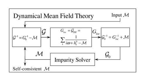
Figure 5: Illustration of the self–consistent cycle in DMFT.

II.1.5 Practical implementation of the self–consistency condition in DMFT.

In many practical calculations, the local Green’s function can be evaluated via Fourier transform. First, given the non–interacting Hamiltonian $h_{\alpha\beta}^{(0)}(\mathbf{k})$, we define the Green’s function in the $\mathbf{k}$–space

$$\mathcal{G}_{\alpha\beta}(\mathbf{k},i\omega)=\left\{[(i\omega+\mu)\hat{O}(\mathbf{k})-\hat{h}^{(0)}(\mathbf{k})-\mathcal{M}_{int}(i\omega)]^{-1}\right\}_{\alpha\beta},$$ (87)

where the overlap matrix $O_{\alpha\beta}(\mathbf{k})$ replaces the unitary matrix $\hat{I}$ introduced earlier in (65) if one takes into account possible non–orthogonality between the basis functions Wegner et al. (2000). Second, the local Green’s function is evaluated as the average in the momentum space

$$G_{loc,\alpha\beta}(i\omega)=\sum_{\mathbf{k}}\mathcal{G}_{\alpha\beta}(\mathbf{k},i\omega),$$ (88)

which can then be used in Eq. (86) to determine the bath Green’s function $\mathcal{G}_{0,\alpha\beta}(i\omega).$

The self–consistency condition in the dynamical mean–field theory requires the inversion of the matrix, Eq. (87) and the summation over $\mathbf{k}$ of an integrand, (88), which in some cases has a pole singularity. This problem is handled by introducing left and right eigenvectors of the inverse of the Kohn–Sham Green’s function

$$\sum_{\beta}\left[h_{\alpha\beta}^{(0)}(\mathbf{k})+\mathcal{M}_{int,\alpha\beta}(i\omega)-\epsilon_{\mathbf{k}j\omega}O_{\alpha\beta}(\mathbf{k})\right]\psi^{R}_{\mathbf{k}j\omega,\beta}=0,\ \$$ (89)

$$\sum_{\alpha}\psi^{L}_{\mathbf{k}j\omega,\alpha}\left[h_{\alpha\beta}^{(0)}(\mathbf{k})+\mathcal{M}_{int,\alpha\beta}(i\omega)-\epsilon_{\mathbf{k}j\omega}O_{\alpha\beta}(\mathbf{k})\right]=0.\ \$$ (90)

This is a non–hermitian eigenvalue problem solved by standard numerical methods. The orthogonality condition involving the overlap matrix is

$$\sum_{\alpha\beta}\psi^{L}_{\mathbf{k}j\omega,\alpha}O_{\alpha\beta}(\mathbf{k})\psi^{R}_{\mathbf{k}j^{\prime}\omega,\beta}=\delta_{jj^{\prime}}.$$ (91)

Note that the present algorithm just inverts the matrix (87) with help of the “right” and “left” eigenvectors. The Green’s function (87) in the basis of its eigenvectors becomes

$$\mathcal{G}_{\alpha\beta}(\mathbf{k},i\omega)=\sum_{j}\frac{\psi^{R}_{\mathbf{k}j\omega,\alpha}\psi^{L}_{\mathbf{k}j\omega,\beta}}{i\omega+\mu-\epsilon_{\mathbf{k}j\omega}}.$$ (92)

This representation generalizes the orthogonal case in the original LDA+DMFT paper Anisimov et al. (1997a). The formula (92) can be safely used to compute the Green’s function as the integral over the Brillouin zone, because the energy denominator can be integrated analytically using the tetrahedron method Lambin and Vigneron (1984).

The self-consistency condition becomes computationally very expensive when many atoms need to be considered in a unit cell, as for example in compounds or complicated crystal structures. A computationally efficient approach was proposed in Ref. Savrasov et al., 2005. If the self-energy is expressed by the rational interpolation in the form

$${\cal M}_{\alpha\beta}(i\omega)={\cal M}_{\alpha}(\infty)\delta_{\alpha\beta}+\sum_{i}\frac{w^{i}_{\alpha\beta}}{i\omega-P_{i}},$$ (93)

where $w^{i}$ are weights and $P_{i}$ are poles of the self-energy matrix. The non-linear Dyson equation (89), (90) can be replaced by a linear Schroedinger-like equation in an extended subset of auxiliary states. This is clear due to mathematical identity

$$\sum_{\mathbf{k}}\left[\begin{array}[]{rr}(i\omega+\mu)\hat{O}_{\mathbf{k}}-\hat{h}^{0}(\mathbf{k})-{\cal M}(\infty),&\sqrt{W}\\ \sqrt{W}^{\dagger},&i\omega-P\end{array}\right]^{-1}=$$ (96)

$$\left[\begin{array}[]{rr}\sum_{\mathbf{k}}\left[{(i\omega+\mu)\hat{O}_{\mathbf{k}}-\hat{h}^{0}(\mathbf{k})-{\cal M}(i\omega)}\right]^{-1},&\cdots\\ \cdots,&\cdots\end{array}\right].$$ (99)

where ${\cal M}(i\omega)$ is given by Eq. (93). Since the matrix $P$ can always be chosen to be a diagonal matrix, we have $w^{i}_{\alpha\beta}=\sqrt{W}_{\alpha i}\sqrt{W}_{\beta i}^{*}$.

The most important advantage of this method is that the eigenvalue problem Eq. (89), (90) does not need to be solved for each frequency separately but only one inversion is required in the extended space including “pole states”. In many applications, only a small number of poles is necessary to reproduce the overall structure of the self-energy matrix (see section III.6.1). In this case, the DMFT self-consistency condition can be computed as fast as solving the usual Kohn-Sham equations.

The situation is even simpler in some symmetry cases. For example, if Hamiltonian is diagonal $h_{\alpha\beta}^{(0)}(\mathbf{k})=\delta_{\alpha\beta}h_{\alpha}^{(0)}(\mathbf{k})$ and the self–energy $\mathcal{M}_{int,\alpha\beta}(i\omega)=\delta_{\alpha\beta}\mathcal{M}_{int,\alpha}(i\omega)$, the inversion in the above equations is trivial and the summation over $\mathbf{k}$ is performed by introducing the non–interacting density of states $N_{\alpha}(\epsilon)$

$$N_{\alpha}(\epsilon)=\sum_{\mathbf{k}}\delta[\epsilon-h_{\alpha}^{(0)}(\mathbf{k})].$$ (100)

The resulting equation for the bath Green’s function becomes

$$\mathcal{G}_{0,\alpha}^{-1}(i\omega)=\left(\int d\epsilon\frac{N_{\alpha}(\epsilon)}{i\omega+\mu-\epsilon-\mathcal{M}_{int,\alpha}(i\omega)}\right)^{-1}+\mathcal{M}_{int,\alpha}(i\omega).$$ (101)

$\bullet$ Assessing the DMFT approximation. Both the dressed atom and the dressed band viewpoint indicate that $\Gamma_{DMFT}$ is going to be a poor approximation to $\Gamma_{SDFT}(G_{loc})$ when interactions are highly nonlocal. However, extensions of the DMFT formalism allow us to tackle this problem. The EDMFT Kajueter (1996b); Kajueter and Kotliar (1996a); Si and Smith (1996) allows us the introduction of long–range Coulomb interactions in the formalism. The short–range Coulomb interaction is more local in the non–orthogonal basis set and can be incorporated using the CDMFT Kotliar et al. (2001).

II.2 Extension to clusters

The notion of locality is not restricted to a single site or a single unit cell, and it is easily extended to a cluster of sites or supercells. We explain the ideas in the context of model Hamiltonians written in an orthogonal basis set to keep the presentation and the notation simple. The extension to general basis sets  Kotliar et al. (2001); Savrasov and Kotliar (2004b) is straightforward.

The motivations for cluster extension of DMFT are multiple: i) Clusters are necessary to study some ordered states like $d$-wave superconductivity which can not be described by a single–site method (Katsnelson and Lichtenstein (2000); Maier et al. (2005); Macridin et al. (2005); Maier et al. (2004b); Maier (2003); Macridin et al. (2004); Maier et al. (2002b, 2000a, 2000a, 2000c)) ii) In cluster methods the lattice self–energies have some $k$ dependence (contrary to single–site DMFT) which is clearly an important ingredient of any theory of the high–$T_{c}$ cuprates for example. Cluster methods may then explain variations of the quasiparticle residue or lifetime along the Fermi surface Parcollet et al. (2004); Civelli et al. (2005) iii) Having a cluster of sites allows the description of non–magnetic insulators (eg. valence bond solids) instead of the trivial non–magnetic insulator of the single–site approach. Similarly, a cluster is needed when Mott and Peierls correlations are simultaneously present leading to dimerization Poteryaev et al. (2004); Biermann et al. (2005b) in which case a correlated link is the appropriate reference frame. iv) The effect of nonlocal interactions within the cluster (e.g. next neighbor Coulomb repulsion) can be investigated Bolech et al. (2003). v) Since cluster methods interpolate between the single–site DMFT and the full problem on the lattice when the size of the cluster increases from one to infinity, they resum $1/d$ corrections to DMFT in a non-perturbative way. Therefore they constitute a systematic way to assert the validity of and improve the DMFT calculations.

Many cluster methods have been studied in the literature. They differ both in the self–consistency condition (how to compute the Weiss bath from the cluster quantities) and on the parameterization of the momentum dependence of the self–energy on the lattice. Different perspectives on single-site DMFT lead to different cluster generalizations : analogy with classical spin systems lead to the Bethe-Peierls approximation Georges et al. (1996), short range approximations of the Baym-Kadanoff functional lead to the “pair scheme”Georges et al. (1996) and its nested cluster generalizations (which reduces to the Cluster Variation Method in the classical limit)Biroli et al. (2004), approximating the self-energy by a piecewise constant function of momentum lead to the dynamical cluster approximation (DCA) Hettler et al. (1998, 2000); Maier et al. (2000c), approximating the self-energy by the lower harmonics lead to the work of Katsnelson and Lichtenstein  Lichtenstein and Katsnelson (2000), and a real space perspective lead to Cellular DMFT (CDMFT). Kotliar et al. (2001). In this review, we focus mainly on the CDMFT method, since it has been used more in the context of realistic computations. For a detailed review of DCA, CDMFT and other schemes and their applications to model Hamiltonians see Maier et al. (2004a).

$\bullet$ Cellular dynamical mean–field theory : definition

The construction of an exact functional of a “local” Green’s function in Eqs. (62), (63),(64) is unchanged, except that the labels $\alpha,\beta$ denotes orbitals and sites within the chosen cluster. The cluster DMFT equations have the form (65), (86), where $\hat{h}^{0}[\mathbf{k}]$ is now replaced by $\hat{t}(K)$ the matrix of hoppings in supercell notation and we use the notation $\Sigma^{\text{C}}(i\omega_{n})$  for the cluster self–energy (note that the notation $\mathcal{M}_{int}$ was used for this quantity in the preceding sections).

$$G_{0}^{-1}(i\omega_{n})=\left(\sum_{K\in RBZ}\Bigl{(}i\omega_{n}+\mu-\hat{t}(K)-\Sigma^{\text{C}}(i\omega_{n})\Bigr{)}^{-1}\right)^{-1}\\ +\Sigma^{\text{C}}(i\omega_{n}),$$ (102)

where the sum over $K$ is taken over the Reduced Brillouin Zone (RBZ) of the superlattice and normalized.

Just like single–site DMFT, one can either view CDMFT as an approximation to an exact functional to compute the cluster Green’s function, or as an approximation to the exact Baym–Kadanoff functional obtained by restricting it to the Green’s functions on the sites restricted to a cluster and its translation by a supercell lattice vector (see Eq. (107) below)  Maier and Jarrell (2002); Georges (2002). From a spectral density functional point of view, Eqs. (66), (67), and the equation $\mathcal{M}_{int}[G]={\delta\Phi_{SDFT}}/{\delta G_{loc}}$ can be viewed as the exact equations provided that the exact functional $\Phi_{SDFT}$ is known.

A good approximation to the “exact functional”, whose knowledge would deliver us the exact cluster Green’s function, is obtained by restricting the exact Baym–Kadanoff functional. In this case, it is restricted to a cluster and all its translations by a supercell vector. Denoting by $C$ the set of couples $(i,j)$ where $i$ and $j$ belong to the same cluster (see Fig. 6 for an example),

$$\Phi^{SDFT}_{CDMFT}=\Phi_{BK}|_{G_{ij}=0\ \mbox{if}\ (i,j)\notin C}$$ (103)

Alternatively the CDMFT equations can be derived from the point of view of a functional of the Weiss field generalizing Eq. (82) from single sites to supercells as shown in Fig. 6. A fundamental concept in DMFT is that of a Weiss field. This is the function describing the environment that one needs to add to an interacting but local problem to obtain the correct local Greens function of an extended system. Now expressed in terms of the Weiss field of the cluster $\mathcal{G}_{0}^{-1}=G_{at}^{-1}-\Delta$. This concept can be used to highlight the connection of the mean field theory of lattice systems with impurity models and the relation of their free energies Georges et al. (1996). For this purpose it is useful to define the DMFT functional of three variables, Kotliar and Savrasov (2001) $G_{loc}$, $\Sigma$ and the Weiss field $\mathcal{G}_{0}$:

$$\Gamma_{CDMFT}[G,\Sigma,{\mathcal{G}_{0}}]=\Sigma_{cells}F_{cell}[{\mathcal{G}_{0}^{-1}}]-\mathrm{Tr}\ln[G]$$ (104)

$$-\mathrm{Tr}\ln[G]\left(i\omega+\mu-{\hat{t}}[k]-\Sigma\right)+\mathrm{Tr}[({\mathcal{G}_{0}}^{-1}-\Sigma-G^{-1})G]\$$

Extremizing this functional gives again the standard CDMFT equations.

$\bullet$ CDMFT : approximation of lattice quantities

The impurity model delivers cluster quantities. In order to make a connection with the original lattice problem, we need to formulate estimates for the lattice Green’s function. A natural way to produce these estimates is by considering the superlattice (SL) (see Fig. 6)

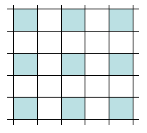
Figure 6: Example of a $2\times 2$ superlattice construction to define CDMFT on a plaquette. Notice that the definition is dependent on the tiling of space by supercells and is therefore not unique

and constructing lattice objects from superlattice objects by averaging the relevant quantities to restore periodicity, namely

$$W_{latt}(i-j)\approx\frac{1}{N_{s}}\sum_{k}~{}W^{SL}_{k,k+i-j},$$ (105)

where $N_{s}$ represents the total number of sites, and $i,j,k$ are site indices. Notice that Eq. (105) represents a super-lattice average, not a cluster average. In particular, if $W$ is the cluster irreducible cumulant, $M_{c}\equiv G_{c}^{-1}+\Delta$ (where $\Delta$ is the hybridization) or the cluster self-energy $\Sigma$ all the contributions with $k$ and $k+i-j$ belonging to different cells are zero by construction. The lattice Greens function can then be reconstructed from the lattice cumulant  Stanescu (2005) or the lattice self-energy  Kotliar et al. (2001); Biroli and Kotliar (2002). Namely $G_{latt}(k,\omega)\approx(\omega-t(k)+\mu-\Sigma_{latt}(k,\omega))^{-1}$ or $G_{latt}(k,\omega)\approx(-t(k)+{M_{latt}(k,\omega)}^{-1})^{-1}$ . Criteria for more general periodizations respecting causality were derived in ref Biroli and Kotliar (2002). Another alternative suggested originally by Sénéchal and Tremblay is to directly periodize the Green’s function, i.e. apply Eq. (105) with $W=G$ to obtain  Senechal et al. (2000)

$${G}({k},\omega)=\frac{1}{N_{c}}\sum_{a,b\in\mathcal{C}}[\hat{M}_{c}^{-1}-\hat{t}_{k}]^{-1}_{ab}~{}e^{i{k}({r}_{a}-{r}_{b})},$$ (106)

where $\hat{t}_{k}$ is the Fourier transform of the “hopping” on the super-lattice, and $N_{c}$ the number of sites in the cluster.

For example, consider the two-dimensional Hubbard model on a square lattice within a four-site approximation (plaquette) in which square symmetry is preserved. After performing the average (105) and then taking the Fourier transform, we obtain the following expressions for the self-energy and the irreducible cumulant of the lattice problem.

$${\Sigma}({k},\omega) = {\Sigma}_{0}(\omega)+{\Sigma}_{1}(\omega)~{}\alpha({k})+{\Sigma}_{2}(\omega)~{}\beta({k}),$$

$${M}({k},\omega) = {M}_{0}(\omega)+{M}_{1}(\omega)~{}\alpha({k})+{M}_{2}(\omega)~{}\beta({k}),$$

where for the cluster quantities $W^{(c)}_{ab}$ we used the notations $W_{0}$ for the on-site values ($a=b$), $W_{1}$ if a and b are nearest neighbors (on a link) and $W_{2}$ if a and b are next-nearest neighbors (on the diagonal), and $\alpha({k})=\cos(k_{x})+\cos(k_{y})$ and $\beta({k})=\cos(k_{x})\cos(k_{y})$.

It is important to notice that it is better to reconstruct on site quantities from the cluster Greens function Capone et al. (2004) and non local quantities from the lattice quantities Stanescu (2005). Using cumulants there is not much difference between estimates from the lattice or the local green function for either one of these quantities, and the same is true about the lattice periodization. Alternatively, periodizing the self-energy has the drawback that the local quantities inferred from $G_{latt}$ differ from $G_{c}$ near the Mott transition.

$\bullet$ Other cluster schemes

We briefly comment on various other cluster schemes mentioned in the introduction (see also Maier et al. (2004a)). Nested cluster schemes are defined by another truncation of the Baym-Kadanoff functional :

$$\Phi^{SDFT}_{Nested}=\Phi_{BK}|_{G_{ij}=0\ \mbox{if}\ (i,j)\notin C}$$ (107)

where $C$ is the set of couples $(i,j)$ with $|i-j|\leq L$ with $L$ is the size of the cluster and we use the Manhattan distance on the lattice. Those schemes combine information from various cluster sizes, and can give very accurate determination of critical temperatures using small cluster sizes, but they are not causal when the range of the self-energy exceeds the size of the truncation Biroli et al. (2004) (See also Okamoto and Millis (2004b)).

There is a class of cluster schemes which are guaranteed to be causal and which requires the solution of one impurity problem : DCA, CDMFT, and PCDMFT (periodized cluster cellular dynamical mean–field theory). The self–consistency condition of all three schemes can be summarized into the same matrix equation

$$G_{0}^{-1}(i\omega_{n})=\Sigma^{\text{C}}(i\omega_{n})+\\ \left(\sum_{K\in RBZ}\Bigl{(}i\omega_{n}+\mu-\hat{t}_{S}(K)-\Sigma_{S}(K,i\omega_{n})\Bigr{)}^{-1}\right)^{-1},$$ (108)

where the difference between the three schemes is enclosed in the value of $t_{S}$ and of $\Sigma_{S}$ that enter in the self–consistency condition. Namely, if $\hat{t}_{S}(K)=\hat{t}(K)$ and $\Sigma_{S}(K,i\omega_{n})=\Sigma^{C}(i\omega_{n})$ we have the CDMFT case, $\hat{t}_{S}(K)=\hat{t}(K)$ and $\Sigma_{S}=\Sigma_{latt}$ corresponds to PCDMFT case, and DCA is realized when $t_{S}(K)=t^{DCA}\equiv t_{\mu\nu}(K)\exp[-iK(\mu-\nu)]$ and $\Sigma_{S}(K,i\omega_{n})=\Sigma^{C}(i\omega_{n})$ Biroli et al. (2004). PCDMFT uses the lattice self–energy in the sum over the reduced Brillouin zone in the self–consistency Eq. (102). It is similar to the scheme proposed by Katsnelson and Lichtenstein  Lichtenstein and Katsnelson (2000), but can be proven to be explicitly causal. The dynamical cluster approximation or DCA Hettler et al. (1998, 2000); Maier et al. (2000c) derives cluster equations starting from momentum space. Its real space formulation of Eq.108 was introduced in Biroli and Kotliar (2002). While in CDMFT (or PCDMFT) the lattice self–energy is expanded on the lowest harmonics in $k$, in DCA the self–energy is taken piecewise constant in the Brillouin Zone.

Simpler approximations, such as cluster perturbation theory (CPT) and variational cluster perturbation theory (VCPT), can also be fruitfully viewed as limiting cases of cluster DMFT. Indeed CPT is obtained by setting the DMFT hybridization equal to zero. The self–energy then becomes the atomic self–energy of the cluster. The lattice self–energy is then obtained by restoring the periodicity in the Green’s function Senechal et al. (2000, 2002); Gros and Valenti (1993); Zacher et al. (2000, 2002); Dahnken et al. (2002). The restriction of the functional (104) to a non zero but static Weiss field, gives rise to the variational cluster perturbation theory (VCPT) introduced in Refs. Potthoff et al. (2003); Senechal and Tremblay (2004); Dahnken et al. (2004). An extensions of these ideas in the context of EDMFT has been recently been carried out by Tong  Tong (2005).

$\bullet$ Hartree–Fock terms

In realistic computations, it is natural to separate the Hartree–Fock term, which can be treated easily from the more complex “exchange” contributions to the Baym–Kadanoff functional $\Phi$. This idea can also be extended to CDMFT, in the case of nonlocal interactions connecting different clusters (e.g. spin–spin interactions). The Hartree–Fock contribution to the Baym–Kadanoff functional induces a self–energy which is frequency independent and therefore does not cause problems with causality and can be evaluated with little computational cost. So it is convenient to separate $\Phi=\Phi_{HF}+\Phi_{int}$, and apply the cluster DMFT truncation only to $\Phi_{int}$, and to the self–energy it generates while treating the Hartree contributions exactly Biroli et al. (2004). More precisely, one can treat with Hartree–Fock terms that connect the cluster to the exterior only, to avoid a double counting problem. This observation is particularly relevant in the treatment of broken symmetries induced by nonlocal interactions as exemplified in the study of the transition to a charge density wave in the extended Hubbard model in one dimension which was studied in Bolech et al. (2003).

$\bullet$ Cluster size dependence

The cluster DMFT methods are in an early stage of development but a few investigations of the performance of the methods for different sizes have already appeared (See Maier et al. (2004a) and references below). There are two distinct issues to consider. The first issue is what can be achieved with very small clusters (e.g. 2 sites in one dimension or 2x2 plaquette in two dimensions). Cluster studies have demonstrated that in a broad region of parameter space, single-site DMFT is quantitatively quite accurate. Similarly, one would like to know what are the minimal clusters needed to capture e.g. the physics of the cuprates. The one–dimensional Hubbard model is a very challenging case to study this question. Application of DMFT and cluster methods to this problem was carried out in Capone et al. (2004) and is reproduced in Figures  7 and  8. Let us note that i) far from the transition, single-site DMFT is quite accurate, ii) a cluster of 2 sites is already very close to the exact solution (obtained by Bethe Ansatz for thermodynamics quantities or DMRG for the dynamical ones). Even though no mean–field approach can produce a Luttinger liquid (a very large cluster would be necessary) CDMFT is shown to perform remarkably well when considering quantities related to intermediate or high energies or associated with the total energy, even near the Mott transition.

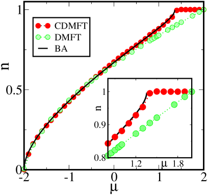
Figure 7: Density $n$ as a function of $\mu$ for the one–dimensional Hubbard model with on–site repulsion strength $U/t=4$, number of cluster sites $N_{c}=2$ within single–site DMFT, two–site CDMFT, two–site PCDMFT and two–site DCA compared with the exact solution by Bethe Ansatz (BA). The lower–right inset shows a region near the Mott transition (adapted from Capone et al. (2004))

.

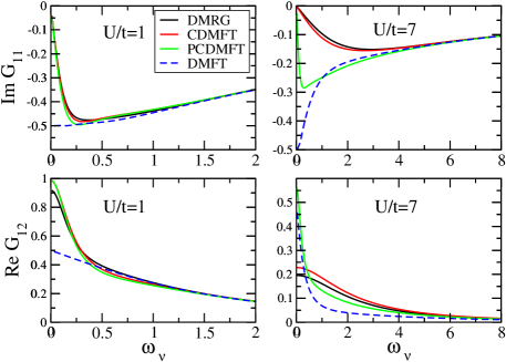
Figure 8: $\Im G_{11}$ and $\Re G_{12}$ for the one–dimensional Hubbard model with on–site repulsion strength $U/t=1$ and $U/t=7$, number of cluster sites $N_{c}=2$ within single–site DMFT, two–site CDMFT, two–site PCDMFT compared with the numerically exact DMRG calculation. (from Capone et al. (2004)).

The second issue is the asymptotic convergence of the methods to the exact solution of the problem (in the infinite cluster limit). At present, this is still a somewhat academic issue because large cluster can not be studied for large $U$ or at low temperature, but algorithmic advances and increase of computer power may change the situation in a near future. The convergence properties of the CDMFT method for large cluster size can be easily improved. Away from critical points, local quantities in CDMFT converge exponentially to their bulk value when measured at the core of the cluster. However, averages over the cluster converge like $1/L$ where $L$ is the linear size of the cluster Biroli and Kotliar (2004) (see also Aryanpour et al. (2005); Biroli and Kotliar (2005)), because in CDMFT the cluster is defined in real space, and the error is maximal and of order 1 in $L$ at the boundary. Therefore, to estimate the value of a local quantity, one should preferentially use the core of the cluster (i.e. giving a lower weight to the boundary) assuming of course that the cluster is large enough to distinguish between a core and a boundary. Failure to do so in CDMFT can lead to non–physical results, as illustrated in the one–dimensional Hubbard model. In this case, the critical temperature for the Néel order does not go to zero when the size of the cluster increases Maier et al. (2002a). In fact, the boundary of a large (chain) cluster sees an effective field given by the other boundary, not by the sites at the center of the cluster, which leads to spurious ordering. It is however possible to greatly improve the convergence properties of CDMFT in ordered phases by weighting the self–energy more at the core of the cluster, a cluster scheme called weighted-CDMFT Parcollet and Kotliar (2005): in the self–consistency condition (102), we replace the self–energy $\Sigma^{\text{C}}$ by $\Sigma^{\text{w}}$

$$\Sigma^{\text{w}}_{\alpha\beta} =\sum_{\alpha^{\prime}\beta^{\prime}}w^{\alpha^{\prime}\beta^{\prime}}_{\alpha\beta}\Sigma^{\text{C}}_{\alpha^{\prime}\beta^{\prime}}$$ (109)

$$w_{\gamma\delta}^{\alpha\beta} =\delta_{\alpha-\beta,\gamma-\delta}f_{c}(\alpha)f_{c}(\beta)$$ (110)

where $f_{c}$ is a normalized function that decays exponentially from the center of the cluster towards the boundaries and satisfy $\sum_{\alpha}f_{c}(\alpha)^{2}=1$. This scheme is causal, it does not present the spurious ordering in one dimension, and it can be shown to have faster convergence of the critical temperature in the classical limit of the Falikov–Kimball model Parcollet and Kotliar (2005). Therefore, for applications to (quasi)-1d systems (chains or ladders) where relatively large cluster size can be reached, weighted-CDMFT should be preferred to CDMFT.

$\bullet$ Numerical solutions

Since the impurity model to be solved for a cluster method is formally a multi-orbital problem, most the solvers used for single-site DMFT can be extended cluster methods, at the expense of an increase of computational cost (See section III). The computational cost of solving the impurity model entering the CDMFT equations using QMC is the same as that of an isolated system of the same cluster, or sometimes even less since it has been found that the presence of the bath reduces the sign problem. To solve the CDMFT equations with exact diagonalization, the bath needs to be discretized and represented by free fermions. This results in an increase in the size of the Hilbert space. $\Delta(\omega)$ has to be represented by a discrete set of poles and, as in single–site DMFT, there are various approaches for choosing a parameterization Georges et al. (1996). A modification of the original procedure of Caffarel and Krauth Caffarel and Krauth (1994) which gives stronger weight to the low–frequency part of the Weiss field has been suggested Capone et al. (2004).

Another possibility for parameterizing the bath is to simply insert a discretized form of the Weiss field into the CDMFT functional, which is viewed as a function of three variables (the obvious generalization of Eq. (II.1.3) to clusters), and varying the functional with respect to the free parameters parameterizing the Weiss field. An alternative choice of the bath parameters can be obtained by inserting approximate expressions of the self-energy parameterized by a few set of parameters into the self-energy functional Potthoff (2003b).

$\bullet$ Application to realistic calculations

In the context of realistic studies of materials, the applications of cluster methods are only beginning. An interesting class of problems are posed by materials with dimerization or charge–charge correlations in the paramagnetic phasei, such as NaV₂O₅. This compound, where the Vanadium atoms are arranged to form two leg ladders which are quarter filled, served as a first application of LDA+DMFT cluster methods. At low temperatures the system is a charge ordered insulator, a situation that is well described by the LDA+U method Yaresko et al. (2000). Above the charge ordering temperature the insulating gap persist, and cluster DMFT is required to describe this unusual insulating state Mazurenko et al. (2002). The second application of this approach focused on the interplay of Pauling- Peierls distortions and Mott correlations Poteryaev et al. (2004) that occur in $Ti_{2}O_{3}$. Titanium sesquioxide, ${Ti}_{2}O_{3}$, is isostructural to Vanadium Sesquioxide, $V_{2}O_{3}$, the prototypical Mott-Hubbard system. In the corundum structure the pair of Titanium atoms form a structural motif. Titanium sesquioxide displays a rapid crossover from a bad metal regime at high temperatures, to an insulating regime at low temperatures. Standard first principles electronic structure methods have failed to account for this crossover. While single site DMFT was quite succesful describing the high temperature physics of $V_{2}O_{3}$ it cannot account for the observed temperature driven crossover in $Ti_{2}O_{3}$ with a reasonable set of parameters. A two site CDMFT calculation with a very reasonable set of onsite interactions and an intersite Coulomb repulsion successfully describes the observed crossover. A surprising result of the cluster calculationsPoteryaev et al. (2004), was the strong frequency dependence of the inter-site Titanium self energy which can be interpret as a scale dependent modification of the bare bonding antibonding splitting. The link reference frame provides an intuitive picture of the synergistic interplay of the lattice distortion (ie. the Pauling -Goodenough-Peierls mechanism Goodenough (1963) which decreases the distance between the Ti atoms) and the Hubbard-Mott mechanism in correlated materials having dimers in the unit cell. The bare (high frequency) parameters of the problem are such that a static mean field calculation yields a metal. However as temperature and frequency are lowered, important correlation effects develop. The bandwidth of the a1g and eg bands is reduced by the correlations while the crystal field splitting between the bonding and the antibonding orbital increases in such a way that the low energy renormalized parameters result in a band insulator. We have a case where the Coulomb interactions enhance the crystal field splitting and reduce the bandwidth, in a synergistic cooperation with the lattice distortions to drive the system thru a metal to insulator crossover.

Another example of the interplay of the Peierls and the Mott mechanism is provided by Vanadium dioxide $VO_{2}$ . This material undergoes a first-order transition from a high-temperature metallic phase to a low-temperature insulating phase near room- temperature. The resistivity jumps by several orders of magnitude through this transition, and the crystal structure changes from rutile at high-temperature to monoclinic at low-temperature. The latter is characterized by a dimerization of the vanadium atoms into pairs, as well as a tilting of these pairs with respect to the c-axis. CDMFT studies of this material Biermann et al. (2005b) can account for the metallic and the insulating phase with reasonable interaction parameters.

II.3 LDA+U method.

We now start the discussion on how the ideas of spectral density functional theory and conventional electronic structure calculations can be bridged together. In many materials, the comparison of LDA calculations with experiment demonstrates that delocalized $s$- and $p$–states are satisfactorily described by local and frequency independent potentials. This leads to the introduction of hybrid methods which separate the electrons into light and heavy. Treating the light electrons using LDA and the heavy electrons using many–body techniques, such as DMFT (see II.4), has already proven to be effective.

As a first illustration, we consider the LDA+U method of Anisimov and co–workers Anisimov et al. (1991). Historically, this was introduced as an extension of the local spin density approximation (LSDA) to treat the ordered phases of the Mott insulating solids. In this respect, the method can be seen as a natural extension of LSDA. However, this method was the first to recognize that a better energy functional can be constructed if not only the density, but also the density matrix of correlated orbitals is brought into the density functional. In this sense, the LDA+U approach is the Hartree–Fock approximation for the spectral density functional within LDA+DMFT, which is discussed in the following section.

$\bullet$ Motivation and choice of variables. From the effective action point of view, the LDA+U constructs a functional of the density $\rho(\mathbf{r}),$ magnetization $\mathbf{m}(\mathbf{r})$, and the occupancy matrix of the correlated orbitals. The latter is defined by projecting the electron creation and destruction operators on a set of local orbitals, $c_{aR}=\int\chi_{a}^{\ast}(\mathbf{r-R})\psi(\mathbf{r})d\mathbf{r},$ i.e. by constructing the occupancy matrix from the local Green’s function

$$n_{ab}=T\sum_{i\omega}e^{i\omega 0^{+}}G_{loc,ab}(i\omega).$$ (111)

In principle, an exact functional of the spin density and the occupancy matrix can be constructed, so as to give the total free energy at the stationary point using the techniques described in previous sections. The LDA+U approximation is an approximate functional of these variables which can be written down explicitly. In the context of LDA+U, the constraining field is designated as $\lambda_{ab}$.

$\bullet$ Form of the functional. The total free energy now is represented as a functional of $\rho(\mathbf{r})$, $\mathbf{m}(\mathbf{r}),$ $n_{ab},$ $\lambda_{ab},$ the Kohn–Sham potential $V_{KS}(\mathbf{r})$ and Kohn–Sham magnetic field, $\mathbf{B}_{KS}(\mathbf{r})$. This representation parallels the Harris–Methfessel form (see Eq. 73). The LDA+U functional is a sum of the kinetic energy, energy related to the external potential and possible external magnetic field, $K_{LDA+U},$ as well as the interaction energy $\Phi_{LDA+U}[\rho,\mathbf{m},n_{ab}]$ (see Kotliar and Savrasov (2001) for more details), i.e.

$$\Gamma_{LDA+U}[\rho,\mathbf{m},n_{ab},\lambda_{ab}]=$$ (112)

$$K_{LDA+U}[\rho,\mathbf{m},n_{ab}]-\lambda_{ab}n_{ab}+\Phi_{LDA+U}[\rho,\mathbf{m},n_{ab}].$$

The form of the functional $K_{LDA+U}$ is analogous to the discussed equations (23), (I.2.2), (68) for the DFT, BK and SDFT theories. The interaction energy $\Phi_{LDA+U}[\rho,\mathbf{m},n_{ab}]$ is represented as follows

$$\Phi_{LDA+U}[\rho,\mathbf{m},n_{ab}]=$$ (113)

$$E_{H}[\rho]+E_{xc}^{LDA}[\rho,\mathbf{m}]+\Phi_{U}^{Model}[n_{ab}]-\Phi_{DC}^{Model}[n_{ab}],$$

This is the LDA interaction energy to which we have added a contribution from the on-site Coulomb energy in the shell of correlated electrons evaluated in the Hartree–Fock approximation

$$\Phi_{U}^{Model}[n_{ab}]=\frac{1}{2}\sum_{abcd\in l_{c}}(U_{acdb}-U_{acbd})n_{ab}n_{cd}.$$ (114)

Here, indexes $a,b,c,d$ involve fixed angular momentum $l_{c}$ of the correlated orbitals and run over magnetic $m$ and spin $\sigma$ quantum numbers. The on–site Coulomb interaction matrix $U_{abcd}$ is the on–site Coulomb interaction matrix element $V_{\alpha=a\beta=b\gamma=c\delta=d}^{RRRR}$ from (59) taken for the sub–block of the correlated orbitals. Since the on-site Coulomb interaction is already approximately accounted for within LDA, the LDA contribution to the on-site interaction needs to be removed. This quantity is referred to as the “double counting” term, and is denoted by $\Phi_{DC}^{Model}[n_{ab}]$. Various forms of the double–counting functional have been proposed in the past. In particular, one of the popular choices is given by Anisimov et al. (1997b)

$$\Phi_{DC}^{Model}[n_{ab}]=\frac{1}{2}\bar{U}\bar{n}_{c}(\bar{n}_{c}-1)-\frac{1}{2}\bar{J}[\bar{n}_{c}^{\uparrow}(\bar{n}_{c}^{\uparrow}-1)+\bar{n}_{c}^{\downarrow}(\bar{n}_{c}^{\downarrow}-1)],$$ (115)

where $\bar{n}_{c}^{\sigma}=\sum_{a\in l_{c}}n_{aa}\delta_{\sigma_{a}\sigma},$ $\bar{n}_{c}=\bar{n}_{c}^{\uparrow}+\bar{n}_{c}^{\downarrow}$ and where $\bar{U}=\frac{1}{(2l_{c}+1)^{2}}\sum_{ab\in l_{c}}U_{abba}$ , $\bar{J}=\bar{U}-\frac{1}{2l_{c}(2l_{c}+1)}\sum_{ab\in l_{c}}(U_{abba}-U_{abab})$.

$\bullet$  Saddle point equations. The Kohn–Sham equations are now obtained by the standard procedure which gives the definitions for the Kohn–Sham potential $V_{KS}(\mathbf{r})$, the effective magnetic field $\mathbf{B}_{KS}(\mathbf{r})$, and the constraining field matrix $\lambda_{ab}.$ The latter is the difference between the orbital–dependent potential $\mathcal{M}_{ab}$ and the contribution due to double counting, $V_{ab}^{DC},$ i.e.

$$\lambda_{ab} = \frac{\delta\Phi_{U}^{Model}}{\delta n_{ab}}-\frac{\delta\Phi_{DC}^{Model}}{\delta n_{ab}}=\mathcal{M}_{ab}-V_{ab}^{DC},$$ (116)

$$\mathcal{M}_{ab} = \sum_{cd}(U_{acdb}-U_{acbd})n_{cd},$$ (117)

$$V_{ab}^{DC} = \delta_{ab}[\bar{U}(\bar{n}_{c}-\frac{1}{2})-\bar{J}(\bar{n}_{c}^{\sigma}-\frac{1}{2})].$$ (118)

$\bullet$ Comments on the parameterization of the functional. (i) The LDA+U functional and the LDA+U equations are defined once a set of projectors and a matrix of interactions $U_{abcd}$ are prescribed. In practice, one can express these matrices via a set of Slater integrals which, for example, for $d$–electrons are given by three constants $F^{(0)},F^{(2)},$ and $F^{(4)}.$ These can be computed from constrained LDA calculations as discussed in Section I.2.5 or taken to be adjustable parameters. An important question is the form of the double counting term $\Phi_{DC}^{Model}$ in Eq. (115). The question arises whether double–counting term should include self–interaction effects or not. In principle, if the total–energy functional contains this spurious term, the same should be taken into account in the double–counting expression. Judged by the experience that the LDA total energy is essentially free of self–interaction (total energy of the hydrogen atom is, for example, very close to –1 Ry, while the Kohn–Sham eigenvalue is only about –0.5 Ry), the construction $\Phi_{DC}^{Model}$ is made such that it is free of the self–interaction. However given the unclear nature of the procedure, alternative forms of the double counting may include the effects of self–interaction. This issue has been reconsidered recently by Petukhov et al. Petukhov et al. (2003) who proposed more general expressions of double counting corrections.

$\bullet$ Assessment of the method. Introducing additional variables into the energy functional allowed for better approximations to the ground–state energy in strongly–correlated situations. This turned out to be a major advance over LDA in situations where orbital order is present. The density matrix for the correlated orbitals is the order parameter for orbital ordering, and its introduction into the functional resembles the introduction of the spin density when going from the LDA to the LSDA.

Unfortunately it suffers from some obvious drawbacks. The most noticeable one is that it only describes spectra which has Hubbard bands when the system is orbitally ordered. We have argued in the previous sections that a correct treatment of the electronic structure of strongly–correlated electron systems has to treat both Hubbard bands and quasiparticle bands on the same footing. Another problem occurs in the paramagnetic phase of Mott insulators: in the absence of broken orbital symmetry, the LDA+U results are very close to the LDA-like solution, and the gap collapses. In systems like NiO where the gap is of the order of several eV, but the Néel temperature is a few hundred Kelvin, it is unphysical to assume that the gap and the magnetic ordering are related.

The drawbacks of the LDA+U method are the same as those of the static Hartree Fock approximation on which it is based. It improves substantially the energetics in situations where a symmetry is broken, but it cannot predict reliably the breaking of a symmetry in some situations. This is clearly illustrated in the context of the Hubbard model where correlation effects reduce the double occupancy, and Hartree Fock can only achieve this effect by breaking the spin system which results in magnetic ordering. For this reason, the LDA+U predicts magnetic order in cases where it is not observed, as, e.g., in the case of Pu Savrasov and Kotliar (2000); Bouchet et al. (2000).

Finally, notice that LDA+U can be viewed as an approximation to the more sophisticated LDA+DMFT treatment consisting of taking the Hartree–Fock approximation for the exchange–correlation functional $\Phi_{DMFT}$ (see (II.4)), which results in a static self–energy. Even in the limit of large interaction $U$, LDA+DMFT does not reduce to LDA+U. For example, LDA+U will incorrectly predict spin ordering temperatures to be on the scale of $U$, while LDA+DMFT correctly predicts them to be on the order of $J$, the exchange interaction. Hence LDA+DMFT captures the local moment regime of various materials (see IV.3), while LDA+U does not.

II.4 LDA+DMFT theory

$\bullet$ Motivation and choice of variables. We now turn to the LDA+DMFT method Anisimov et al. (1997a); Lichtenstein and Katsnelson (1998). This approach can be motivated from different perspectives. It can be viewed as a natural evolution of the LDA+U method to eliminate some of its difficulties. It can also be viewed as a way to upgrade the DMFT approach, which so far has been applied to model Hamiltonians, in order to bring in realistic microscopic details.

To compute the energy in a combination of LDA and DMFT one can use an approximate formula to avoid the overcounting of the free energy $F_{tot}=F_{LDA}+F_{DMFT}-F_{mLDA}$ where $F_{mLDA}$ is a mean–field treatment of the LDA Hamiltonian. This procedure was used by Held et al. in their work on Cerium Held et al. (2001b). Alternatively, the approach proposed in this section uses an effective action construction and obtains an approximate functional merging LDA and DMFT. This has the advantage of offering in principle stationarity in the computation of the energy.

In this review we have built a hierarchy of theories, which focus on more refined observables (see Table 1). At the bottom of the hierarchy we have the density functional theory which focuses on the density, and at the top of the hierarchy we have a Baym–Kadanoff approach which focuses on the full electronic Green’s function. The LDA+DMFT is seen as an intermediate theory, which focuses on two variables, the density and the local Green’s function of the heavy electrons. It can be justified by reducing theories containing additional variables, a point of view put forward recently in Ref. Savrasov and Kotliar, 2004b.

Method	Physical Quantity	Constraining Field
Baym–Kadanoff	$G_{\alpha\beta}(\mathbf{k},i\omega)$	$\Sigma_{int,\alpha\beta}(\mathbf{k},i\omega)$
DMFT (BL)	$G_{loc,\alpha\beta}(i\omega)$	$\mathcal{M}_{int,\alpha\beta}(i\omega)$
DMFT (AL)	$G_{loc,\alpha\beta}(i\omega)$	$\Delta_{\alpha\beta}(i\omega)$
LDA+DMFT (BL)	$\rho(r),G_{loc,ab}(i\omega)$	$V_{int}(r),\mathcal{M}_{int,ab}(i\omega)$
LDA+DMFT (AL)	$\rho(r),G_{loc,ab}(i\omega)$	$V_{int}(r),\Delta_{ab}(i\omega)$
LDA+U	$\rho(r),n_{ab}$	$V_{int}(r),\lambda_{ab}$
LDA	$\rho(r)$	$V_{int}(r)$

Table 1: Parallel between the different approaches, indicating the physical quantity which has to be extremized, and the field which is introduced to impose a constraint (constraining field). (BL) means band limit and (AL) corresponds to atomic limit.

$\bullet$ Construction of the exact functional. We derive the equations following the effective action point of view Chitra and Kotliar (2001). To facilitate the comparison between the approaches discussed in the earlier sections we have tabulated (see Table 1) the central quantities which have to be minimized, and the fields which are introduced to impose a constraint in the effective action method Fukuda et al. (1994). As in the LDA+U method one introduces a set of correlated orbitals $\chi_{a}(\mathbf{r}-\mathbf{R}).$ One defines an exact functional of the total density $\rho(x)$ and of the local spectral function of the correlated orbitals discussed before:

$$G_{loc,ab}(\tau,\tau^{\prime})=-\int\sum_{R}\chi_{Ra}(\mathbf{r})\left\langle\psi(x)\psi^{+}(x^{\prime})\right\rangle\chi_{Rb}^{\ast}(\mathbf{r}^{\prime})d\mathbf{r}d\mathbf{r}^{\prime}$$ (119)

where indexes $a,b$ refer exclusively to the correlated orbitals, and $c_{Rb}^{+}$ creates $\chi_{b}(\mathbf{r}-\mathbf{R}).$.

We now introduce the sources for the density, $L(x)$, and for the local spectral function of the correlated orbitals, $J_{loc,Rab}(\tau,\tau^{\prime}).$ These two sources modify the action as follows

$$S^{\prime}=S+\int L(x)\psi^{+}(x)\psi(x)dx+$$ (120)

$$\frac{1}{N}\sum_{Rab}\int J_{loc,Rab}(\tau\mathbf{,}\tau^{\prime})c_{Ra}^{+}(\tau)c_{Rb}(\tau^{\prime})d\tau d\tau^{\prime}.$$

This defines the free energy of the system as a functional of the source fields after (33). Both density and local Green’s function can be calculated as follows

$$\frac{\delta F}{\delta L(x)}=\rho(x),$$ (121)

$$\frac{\delta F}{\delta J_{loc,Rba}(\tau^{\prime}\mathbf{,}\tau)\ }=G_{loc,ab}(\tau\mathbf{,}\tau^{\prime}).$$ (122)

Then, the functional of both density and the spectral function is constructed by the Legendre transform. This is an exact functional of the density and the local Green’s function, $\Gamma(\rho,G_{loc})$, which gives the exact total free energy, the exact density, and the exact local Green’s function of the heavy electrons at the stationary point.

$\bullet$ Exact representations of the constraining field. A perturbative construction can be carried out either around the atomic limit or around the band limit following the inversion method. Unfortunately the latter is very involved and has not been yet evaluated, except for the lowest order (so–called “tree”) level neglecting nonlocal interactions. One can also perform a decomposition into the lowest order term (consisting of “kinetic energy”) and the rest (with an exchange and correlation energy).

$\bullet$ Constructing approximations. Given that DMFT has proven to accurately describe many systems at the level of model Hamiltonians, and that LDA has a long history of success in treating weakly correlated materials, LDA+DMFT is obviously a reasonable choice for an approximation to the exact functional.

The functional implementation corresponding to this approximation is given by $\Gamma_{LDA+DMFT}$ and has the form

$$\Gamma_{LDA+DMFT}[\rho,G_{loc},V_{int},\mathcal{M}_{int}]=$$

$$-\mathrm{Tr}\ln[i\omega+\mu+\nabla^{2}-V_{ext}-V_{int}-\sum_{abR}[\mathcal{M}_{int,ab}(i\omega)-\mathcal{M}_{DC,ab}]\chi_{a}(\mathbf{r-R})\chi_{b}^{\ast}(\mathbf{r}^{\prime}-\mathbf{R})]$$ (123)

$$-\int V_{int}(\mathbf{r})\rho(\mathbf{r})d\mathbf{r}-T\sum_{i\omega}\sum_{ab}[\mathcal{M}_{int,ab}(i\omega)-\mathcal{M}_{DC,ab}]G_{loc,ba}(i\omega)+E_{H}[\rho]+E_{xc}^{LDA}[\rho]+\Phi_{DMFT}[G_{loc,ab}]-\Phi_{DC}[n_{ab}].$$

$\Phi_{DMFT}[G_{loc,ab}]$ is the sum of all two–particle irreducible graphs constructed with the local part of the interaction and the local Green’s function, and $\Phi_{DC}[n_{ab}]$ is taken to have the same form as in the LDA+U method, Eq. (115). In a fixed tight–binding basis, $-\nabla^{2}+V_{ext}$ reduces to $h_{ab}^{(0)}(\mathbf{k})$ and the functional $\Gamma_{LDA+DMFT}$ Eq. (II.4), for a fixed density truncated to a finite basis set, takes a form identical to the DMFT functional which was discussed in Section II.1.

$\bullet$ Saddle point equations. Minimization of the functional leads to the set of equations with the Kohn–Sham potential and

$$\mathcal{M}_{int,ab}(i\omega) = \frac{\delta\Phi_{DMFT}}{\delta G_{loc,ba}(i\omega)},$$ (124)

$$\mathcal{M}_{DC,ab} = \frac{\delta\Phi_{DC}}{\delta n_{ba}},$$ (125)

which identifies matrix $\mathcal{M}_{int,ab}(i\omega)$ as the self–energy of the generalized Anderson impurity model in a bath characterized by a hybridization function $\Delta_{ab}(i\omega)$ obeying the self–consistency condition

$$(i\omega+\mu)\bar{O}_{ab}-\bar{\epsilon}_{ab}-\Delta_{ab}(i\omega)-\mathcal{M}_{int,ab}(i\omega)=$$ (126)

$$\left[\sum_{\mathbf{k}}[(i\omega+\mu)\hat{O}(\mathbf{k})-\hat{h}^{(LDA)}(\mathbf{k})-\mathcal{M}_{int}(i\omega)+\mathcal{M}_{DC}]^{-1}\right]_{ab}^{-1}.$$

By examining the limiting behavior $i\omega\rightarrow\infty$, we get the definition of the average overlap matrix $\bar{O}_{ab}$ for the impurity levels as inverse of the average inverse overlap, i.e.

$$\bar{O}_{ab}=\left[\sum_{\mathbf{k}}\hat{O}^{-1}(\mathbf{k})\right]_{ab}^{-1}.$$ (127)

Similarly, the matrix of the impurity levels has the following form

$$\bar{\epsilon}_{ab}=\sum_{cd}\bar{O}_{ac}\left[\sum_{\mathbf{k}}\hat{O}^{-1}(\mathbf{k})[h^{(LDA)}(\mathbf{k})+\mathcal{M}_{int}(i\infty)-\mathcal{M}_{DC}]\hat{O}^{-1}(\mathbf{k})\right]_{cd}\bar{O}_{db}-\mathcal{M}_{int,ab}(i\infty).$$ (128)

Finally, minimization of Eq. (II.4) with respect to $V_{eff}$ indicates that $\rho(\mathbf{r})$ should be computed as follows

$$\rho(\mathbf{r})=T\sum_{i\omega}\left\langle\mathbf{r}\left|[i\omega+\mu+\nabla^{2}-V_{eff}-\sum_{abR}[\mathcal{M}_{int,ab}(i\omega)-\mathcal{M}_{DC,ab}]\chi_{a}(\mathbf{r-R})\chi_{b}^{\ast}(\mathbf{r}^{\prime}-\mathbf{R})]^{-1}\right|\mathbf{r}\right\rangle e^{i\omega 0^{+}}.$$ (129)

The self–consistency in the LDA+DMFT theory is performed as a double iteration loop, the inside loop is over the DMFT cycle and the outside loop is over the electron density, which modifies the one–electron LDA Hamiltonian. The self–consistent cycle is illustrated in Fig. 9.

$\bullet$Evaluation of the total energy. In general, the free energy is $F_{tot}=E_{tot}-TS,$ where $E_{tot}$ is the total energy and $S$ is the entropy. Both energy and entropy terms exist in the kinetic and interaction functionals. The kinetic energy part of the functional is given by $K_{SDFT}[\mathcal{G}]=\mathrm{Tr(}-\nabla^{2}+V_{ext})\mathcal{G}$ while the potential energy part is $\frac{1}{2}\mathrm{Tr}\mathcal{M}_{int}G_{loc}$ therefore the total energy within LDA+DMFT becomes

$$E_{tot} = T\sum_{\mathbf{k}j}\sum_{i\omega}g_{\mathbf{k}j\omega}\epsilon_{\mathbf{k}j\omega}-\int V_{int}(\mathbf{r})\rho(\mathbf{r})d\mathbf{r}-T\sum_{i\omega}\sum_{ab}[\mathcal{M}_{int,ab}(i\omega)-\mathcal{M}_{DC,ab}]G_{loc,ba}(i\omega)+$$ (130)

$$+E_{H}[\rho]+E_{xc}^{LDA}[\rho]+\frac{1}{2}T\sum_{i\omega}\sum_{ab}\mathcal{M}_{int,ab}(i\omega)G_{loc,ba}(i\omega)-\Phi_{DC}[n_{ab}],$$

where the frequency–dependent eigenvalues $\epsilon_{\mathbf{k}j\omega}$ come as a result of diagonalizing the following non–hermitian eigenvalue problem similar to (89):

$$\sum_{\beta}\left[h_{\alpha\beta}^{(LDA)}(\mathbf{k})+\delta_{\alpha a}\delta_{\beta b}(\mathcal{M}_{int,ab}(i\omega)-\mathcal{M}_{DC,ab})-\right.$$

$$\left.\epsilon_{\mathbf{k}j\omega}O_{\alpha\beta}(\mathbf{k})\right]\psi^{R}_{\mathbf{k}j\omega,\beta}=0.$$ (131)

Also,

$$g_{\mathbf{k}j\omega}=\frac{1}{i\omega+\mu-\epsilon_{\mathbf{k}j\omega}},$$ (132)

is the Green’s function in the orthogonal left/right representation which plays a role of a “frequency–dependent occupation number”.

Figure 9: Illustration of self–consistent cycle in spectral density functional theory with LDA+DMFT approximation: double iteration cycle consists of the inner DMFT loop and outer (density plus total energy) loop.

Evaluation of the entropy contribution to the free energy can be performed by finding the total energy at several temperatures and then taking the integral Georges et al. (1996)

$$S(T)=S(\infty)-\int_{T}^{\infty}dT^{\prime}\frac{1}{T^{\prime}}\frac{dE_{LDA+DMFT}}{dT^{\prime}}.$$ (133)

The infinite temperature limit $S(\infty)$ for a well defined model Hamiltonian can be worked out. This program was implemented for the Hubbard model Rozenberg et al. (1994) and for Ce Held et al. (2001b). If we are not dealing with a model Hamiltonian construction  one has to take instead of infinity a sufficiently high temperature so that the entropy $S(\infty)$ can be evaluated by semiclassical considerations.

$\bullet$ Choice of basis and double counting. The basis can be gradually refined so as to obtain more accurate solutions in certain energy range. In principle this improvement is done by changing the linearization energies, and the experience from density functional implementations could be carried over to the DMFT case.

Notice that the rational for the double counting term described in Eq. (115) was chosen empirically to fit the one–particle spectra of Mott insulator (for further discussion see Petukhov et al. (2003)) and deserves further investigations. All the discussion of double counting terms in LDA+U literature can be extended to LDA+DMFT. Notice that as long as the equations are derivable from a functional, the Luttinger theorem is satisfied (in the single–site DMFT case).

In addition to the forms of double counting terms discussed in Section II.3, it has been proposed to use the DMFT self–energy at zero or at infinity for the double counting. One possibility

$$\mathcal{M}_{DC,ab}=\frac{1}{N_{\deg}}\delta_{ab}\sum_{a^{\prime}}\mathcal{M}_{int,a^{\prime}a^{\prime}}(0),$$ (134)

was suggested and implemented by Lichtenstein et al. in their work on Fe and Ni Lichtenstein et al. (2001). The spin polarized version of this term, has been recently applied to Iron with encouraging results Katsnelson and Lichtenstein (2000).

$\bullet$ Assessment of the LDA+DMFT method. The addition of a realistic band theory to the DMFT treatment of models of correlated electron systems has opened a new area of investigations. To the many–body theorist, the infusion of a realistic band theory allows one to make system–specific studies. Some of them are listed in Section IV on materials. For the electronic structure community, the LDA+DMFT method allows the treatment of a variety of materials which are not well treated by the LDA or the LDA+U method, such as correlated metals and systems with paramagnetic local moments. The main shortcoming is in the arbitrariness in the choice of the correlated orbitals, in the estimation of the $U$, and the ambiguity in the choice of double counting correction. This may turn out to be hard to resolve within this formalism. The ideas described in the following section formulate the many–body problem in terms of fluctuating electric fields and electrons, treat all the electrons on the same footing, provide an internally consistent evaluation of the interaction, and eliminate the need for the double counting correction.

II.5 Equations in real space

$\bullet$ Functional of the local Green’s function in real space. The success of the dynamical mean–field approximations is related to the notion that the local approximation is good in many situations. Thus far, the notion of locality has only been explored after choosing a set of tight–binding orbitals, but it can also be formulated directly in real space, as stressed recently in Ref. Savrasov and Kotliar (2004b); Chitra and Kotliar (2000a). This is necessary in order to make direct contact with theories such as density functional theory, which is formulated directly in the continuum without resorting to a choice of orbitals or preferred basis set. The theory is formulated by defining the local Green’s function to be the exact Green’s function $G(\mathbf{r},\mathbf{r}^{\prime},z)$ within a given volume $\Omega_{loc}$ and zero outside. In other words,

$$G_{loc}(\mathbf{r},\mathbf{r}^{\prime},z)=G(\mathbf{r},\mathbf{r}^{\prime},z)\theta_{loc}(\mathbf{r},\mathbf{r}^{\prime}),$$ (135)

where $\mathbf{r}$ is within a primitive unit cell $\Omega_{c}$ positioned at $\mathbf{R}=0$ while $\mathbf{r}^{\prime}$ travels within some volume $\Omega_{loc}$ centered at $\mathbf{R}=0$. Theta function is unity when $\mathbf{r}\in\Omega_{c},\mathbf{r}^{\prime}\in\Omega_{loc}$ and zero otherwise. This construction can be translationally continued onto entire lattice by enforcing the property $\theta_{loc}(\mathbf{r+R},\mathbf{r}^{\prime}+\mathbf{R})=\theta_{loc}(\mathbf{r},\mathbf{r}^{\prime}).$

The procedures outlined in the previous sections can be applied to the continuum in order to construct an exact functional which gives the exact free energy, the local Green’s function (in real space), its Kohn–Sham  formulation, and its dynamical mean–field approximation (by restricting the interaction in the full Baym–Kadanoff functional to the local Green’s function).

This approach has the advantage that the density is naturally contained in this definition of a local Green’s function, and therefore the density functional theory is naturally embedded in this formalism. Another advantage is that the approach contains the bare Coulomb interaction, and therefore is free from phenomenological parameters such as the Hubbard $U$. However, this may create problems since it is well–known that significant screening of the interactions occurs within real materials. Therefore, it is useful to incorporate the effects of screening at a level of functional description of the system.

$\bullet$ Motivation and choice of variables: spectral density functional of the local Green’s functions and of the local interaction. We introduce two local source fields $J_{loc}$ and $K_{loc}$ which probe the local electron Green’s function $G_{loc}$ defined earlier and the local part of the boson Green’s function $W_{loc}(x,x^{\prime})=\langle T_{\tau}\phi(x)\phi(x^{\prime})\rangle\theta_{loc}(\mathbf{r},\mathbf{r}^{\prime})$ being the screened interaction (see Section I.2.3). This generalization represents the ideas of the extended dynamical mean–field theory Si and Smith (1996), now viewed as an exact theory. Note that formally the cluster for the interaction can be different from the one considered to define the local Green’s function (135) but we will not distinguish between them for simplicity. The auxiliary Green’s function $\mathcal{G}(\mathbf{r},\mathbf{r}^{\prime},i\omega)$ as well as the auxiliary interaction $\mathcal{W}(\mathbf{r},\mathbf{r}^{\prime},i\omega)$ are introduced which are the same as the local functions within non–zero volume of $\theta_{loc}(\mathbf{r},\mathbf{r}^{\prime})$

$$G_{loc}(\mathbf{r},\mathbf{r}^{\prime},i\omega) = \mathcal{G}(\mathbf{r},\mathbf{r}^{\prime},i\omega)\theta_{loc}(\mathbf{r},\mathbf{r}^{\prime}),$$ (136)

$$W_{loc}(\mathbf{r},\mathbf{r}^{\prime},i\omega) = \mathcal{W}(\mathbf{r},\mathbf{r}^{\prime},i\omega)\theta_{loc}(\mathbf{r},\mathbf{r}^{\prime}).$$ (137)

The spectral density functional is represented in the form

$$\Gamma_{SDFT}[G_{loc},W_{loc}]=Tr\ln\mathcal{G}-Tr[G_{0}^{-1}-\mathcal{G}^{-1}]\mathcal{G+}E_{H}[\rho]-\frac{1}{2}\mathrm{Tr}\ln\mathcal{W}+\frac{1}{2}\mathrm{Tr}[v_{C}^{-1}-\mathcal{W}^{-1}]\mathcal{W}+\Psi_{SDFT}[G_{loc},W_{loc}].$$ (138)

It can be viewed as a functional $\Gamma_{SDFT}[G_{loc},W_{loc}]$ or alternatively as a functional $\Gamma_{SDFT}[\mathcal{G},\mathcal{W}]$. $\Psi_{SDFT}[G_{loc},W_{loc}]$ is formally not a sum of two–particle diagrams constructed with $G_{loc}\$and $W_{loc}$, but in principle a more complicated diagrammatic expression can be derived following Refs. Fukuda et al. (1994); Valiev and Fernando (1997); Chitra and Kotliar (2001). A more explicit expression involving a coupling constant integration can be given. Examining stationarity of $\Gamma_{SDFT}$ yields saddle–point equations for $\mathcal{G}(\mathbf{r},\mathbf{r}^{\prime},i\omega)$ and for $\mathcal{W}(\mathbf{r},\mathbf{r}^{\prime},i\omega)$

$$\mathcal{G}^{-1}(\mathbf{r},\mathbf{r}^{\prime},i\omega) = G_{0}^{-1}(\mathbf{r},\mathbf{r}^{\prime},i\omega)-\mathcal{M}_{int}(\mathbf{r},\mathbf{r}^{\prime},i\omega),\ \ \ \ \ \$$ (139)

$$\mathcal{W}^{-1}(\mathbf{r},\mathbf{r}^{\prime},i\omega) = v_{C}^{-1}(\mathbf{r}-\mathbf{r}^{\prime})-\mathcal{P}(\mathbf{r},\mathbf{r}^{\prime},i\omega),$$ (140)

where $\mathcal{M}_{int}(\mathbf{r},\mathbf{r}^{\prime},i\omega)$ is the auxiliary local mass operator defined as the variational derivative of the interaction functional:

$$\mathcal{M}_{int}(\mathbf{r},\mathbf{r}^{\prime},i\omega)=\frac{\delta\Phi_{SDFT}[G_{loc}]}{\delta\mathcal{G}(\mathbf{r}^{\prime},\mathbf{r},i\omega)}=\frac{\delta\Phi_{SDFT}[G_{loc}]}{\delta G_{loc}(\mathbf{r}^{\prime},\mathbf{r},i\omega)}\theta_{loc}(\mathbf{r},\mathbf{r}^{\prime}),$$ (141)

$\mathcal{P}(\mathbf{r},\mathbf{r}^{\prime},i\omega)$ is the effective susceptibility of the system defined as the variational derivative

$$\mathcal{P}(\mathbf{r},\mathbf{r}^{\prime},i\omega)=\frac{-2\delta\Psi_{SDFT}}{\delta\mathcal{W}(\mathbf{r}^{\prime},\mathbf{r},i\omega)}=\frac{-2\delta\Psi_{SDFT}}{\delta W_{loc}(\mathbf{r}^{\prime},\mathbf{r},i\omega)}\theta_{loc}(\mathbf{r},\mathbf{r}^{\prime}).$$ (142)

Notice again a set of parallel observations for $\mathcal{P}$ as for $\mathcal{M}_{int}$. Both $\mathcal{P}$ and $\mathcal{M}_{int}$ are local by construction, i.e. these are non–zero only within the cluster restricted by $\theta_{loc}(\mathbf{r},\mathbf{r}^{\prime}).$ Formally, they are auxiliary objects and cannot be identified with the exact self–energy and susceptibility of the electronic system. However, if the exact self–energy and susceptibility are sufficiently localized, this identification becomes possible. If the cluster $\Omega_{loc}$ includes the physical area of localization, we can immediately identify $\mathcal{M}_{int}(r,r^{\prime},i\omega)$ with $\Sigma_{int}(\mathbf{r},\mathbf{r}^{\prime},i\omega),$ $\mathcal{P}(\mathbf{r},\mathbf{r}^{\prime},i\omega)$ with $\Pi(\mathbf{r},\mathbf{r}^{\prime},i\omega)$ in all space. However, both $\mathcal{G}(\mathbf{r},\mathbf{r}^{\prime},i\omega)$ and $G(\mathbf{r},\mathbf{r}^{\prime},i\omega)$ as well as $\mathcal{W}$ and $W$ are always the same within $\Omega_{loc}$ regardless its size, as it is seen from (136) and (137).

$\bullet$ Practical implementation and Kohn–Sham representation. The Kohn–Sham Green’s function can be calculated using the following representation

$$\mathcal{G}(\mathbf{r},\mathbf{r}^{\prime},i\omega)=\sum_{\mathbf{k}j}\frac{\psi_{\mathbf{k}j\omega}^{R}(\mathbf{r})\psi_{\mathbf{k}j\omega}^{L}(\mathbf{r}^{\prime})}{i\omega+\mu-\epsilon_{\mathbf{k}j\omega}},$$ (143)

where the left $\psi_{\mathbf{k}j\omega}^{L}(\mathbf{r})$ and right $\psi_{\mathbf{k}j\omega}^{R}(\mathbf{r})$ states satisfy the following Dyson equations

$$[-\nabla^{2}+V_{ext}(\mathbf{r})+V_{H}(\mathbf{r})]\psi_{\mathbf{k}j\omega}^{R}(\mathbf{r})+\int\mathcal{M}_{xc}(\mathbf{r},\mathbf{r}^{\prime},i\omega)\psi_{\mathbf{k}j\omega}^{R}(\mathbf{r}^{\prime})d\mathbf{r}^{\prime} = \epsilon_{\mathbf{k}j\omega}\psi_{\mathbf{k}j\omega}^{R}(\mathbf{r}),$$ (144)

$$[-\nabla^{2}+V_{ext}(\mathbf{r}^{\prime})+V_{H}(\mathbf{r}^{\prime})]\psi_{\mathbf{k}j\omega}^{L}(\mathbf{r}^{\prime})+\int\psi_{\mathbf{k}j\omega}^{L}(\mathbf{r})\mathcal{M}_{xc}(\mathbf{r},\mathbf{r}^{\prime},i\omega)d\mathbf{r} = \epsilon_{\mathbf{k}j\omega}\psi_{\mathbf{k}j\omega}^{L}(\mathbf{r}^{\prime}).$$ (145)

These equations should be considered as eigenvalue problems with a complex, non–hermitian self–energy. As a result, the eigenvalues $\epsilon_{\mathbf{k}j\omega}$ are complex in general, and the same for both equations. The explicit dependence on the frequency $i\omega$ of both the eigenvectors and eigenvalues comes from the self–energy. Note that left and right eigenfunctions are orthonormal

$$\int d\mathbf{r}\psi_{\mathbf{k}j\omega}^{L}(\mathbf{r})\psi_{\mathbf{k}j^{\prime}\omega}^{R}(\mathbf{r})\mathbf{=}\delta_{jj^{\prime}},$$ (146)

and can be used to evaluate the charge density of a given system using the Matsubara sum and the integral over the momentum space

$$\rho(\mathbf{r})=T\sum_{i\omega}\sum_{\mathbf{k}j}\frac{\psi_{\mathbf{k}j\omega}^{R}(\mathbf{r})\psi_{\mathbf{k}j\omega}^{L}(\mathbf{r})}{i\omega+\mu-\epsilon_{\mathbf{k}j\omega}}e^{i\omega 0^{+}}.$$ (147)

It can be shown Savrasov and Kotliar (2004b) that this system of equations reduces to the Kohn–Sham eigensystem when the self–energy is frequency independent.

Note that the frequency–dependent energy bands $\epsilon_{\mathbf{k}j\omega}$ represent an auxiliary set of complex eigenvalues. These are not the true poles of the exact one–electron Green’s function $G(\mathbf{r},\mathbf{r}^{\prime},z)$. However, they are designed to reproduce the local spectral density of the system. Note also that these bands $\epsilon_{\mathbf{k}jz}$ are not the true poles of the auxiliary Green’s function $\mathcal{G}(\mathbf{r},\mathbf{r}^{\prime},z)$. Only in the situation when $\mathcal{G}$ is a good approximation to $G$, the solution of the equation $z+\mu-\epsilon_{\mathbf{k}jz}=0$ gives a good approximation for the quasiparticle energies

$\bullet$ Evaluation of the total energy. The energy–dependent representation allows one to obtain a very compact expression for the total energy. As we have argued, the entropy terms are more difficult to evaluate. However, as long as we stay at low temperatures, these contributions are small and the total energy approach is valid. In this respect, the SDFT total energy formula is obtained by utilizing the relationship $\epsilon_{\mathbf{k}j\omega}=\langle\psi_{\mathbf{k}j\omega}^{L}|-\nabla^{2}+\mathcal{M}_{eff}|\psi_{\mathbf{k}j\omega}^{R}\rangle=\langle\psi_{\mathbf{k}j\omega}^{L}|-\nabla^{2}+V_{ext}+V_{H}+\mathcal{M}_{xc}|\psi_{\mathbf{k}j\omega}^{R}\rangle$

$$E_{SDFT}=T\sum_{i\omega}e^{i\omega 0^{+}}\sum_{\mathbf{k}j}g_{\mathbf{k}j\omega}\epsilon_{\mathbf{k}j\omega}-T\sum_{i\omega}\int d\mathbf{r}d\mathbf{r}^{\prime}\mathcal{M}_{eff}(\mathbf{r,r}^{\prime},i\omega)\mathcal{G}(\mathbf{r}^{\prime},\mathbf{r},i\omega)+$$

$$+\int d\mathbf{r}V_{ext}(\mathbf{r})\rho(\mathbf{r})+E_{H}[\rho]+\frac{1}{2}T\sum_{i\omega}\int d\mathbf{r}d\mathbf{r}^{\prime}\mathcal{M}_{xc}(\mathbf{r,r}^{\prime},i\omega)G_{loc}(\mathbf{r}^{\prime},\mathbf{r},i\omega),$$ (148)

where $\mathcal{M}_{eff}=\mathcal{M}_{int}+V_{ext}$ and $g_{\mathbf{k}j\omega}=1/(i\omega+\mu-\epsilon_{\mathbf{k}j\omega})$. For the same reason as in DFT, this expression should be evaluated with the value of the the self-energy $\mathcal{M}_{eff}$ which is used as input to the routine performing the inversion of the Dyson equation, and with the value of the Green’s function $\cal G$ which is the output of that inversion.

$\bullet$ Constructions of approximations. The dynamical mean–field approximation to the exact spectral density functional is defined by restricting the interaction part of Baym–Kadanoff functional $\Psi_{SDFT}[G_{loc},W_{loc}]$ to $G_{loc}(\mathbf{r},\mathbf{r}^{\prime},z)$ and $W_{loc}(\mathbf{r},\mathbf{r}^{\prime},i\omega).$ The sum over all the diagrams, constrained to a given site, together with the Dyson equations can be formulated in terms of the solution of an auxiliary Anderson impurity model, after the introduction of a basis set. We introduce a bath Green’s function $\mathcal{G}_{0}(\mathbf{r},\mathbf{r}^{\prime},i\omega)$ and a “bath interaction” $\mathcal{V}_{0}(\mathbf{r},\mathbf{r}^{\prime},i\omega)$ defined by the following Dyson equations

$$\mathcal{G}_{0}^{-1}(\mathbf{r},\mathbf{r}^{\prime},i\omega) = G_{loc}^{-1}(\mathbf{r},\mathbf{r}^{\prime},i\omega)+\mathcal{M}_{int}(\mathbf{r},\mathbf{r}^{\prime},i\omega),\ \ \ \ \$$ (149)

$$\mathcal{V}_{0}^{-1}(\mathbf{r},\mathbf{r}^{\prime},i\omega) = W_{loc}^{-1}(\mathbf{r},\mathbf{r}^{\prime},i\omega)+\mathcal{P}(\mathbf{r},\mathbf{r}^{\prime},i\omega).$$ (150)

Note that formally neither $\mathcal{G}_{0}$ nor $\mathcal{V}_{0}$ can be associated with non–interacting $G_{0}$ and the bare interaction $v_{C},$ respectively. These two functions are to be considered as an input to the auxiliary impurity model which delivers new $\mathcal{M}_{int}(\mathbf{r},\mathbf{r}^{\prime},i\omega)$ and $\mathcal{P}(\mathbf{r},\mathbf{r}^{\prime},i\omega).$

To summarize, the effective impurity action, the Dyson equations (149), (150) connecting local and bath quantities as well as the original Dyson equations (139), (140) constitute a self–consistent set of equations as the saddle–point conditions extremizing the spectral density functional $\Gamma_{SDFT}(\mathcal{G},\mathcal{W})$. They combine cellular and extended versions of DMFT and represent our philosophy in the ab initio simulation of a strongly–correlated system. Since $\mathcal{M}_{int}$ and $\mathcal{P}$ are unknown at the beginning, the solution of these equations assumes self–consistency. First, assuming some initial $\mathcal{M}_{int}$ and $\mathcal{P}$, the original Dyson equations (139), (140) are used to find Green’s function $\mathcal{G}$ and screened interaction $\mathcal{W}.$ Second, the Dyson equations for the local quantities (149), (150) are used to find $\mathcal{G}_{0}$, $\mathcal{V}_{0}.$ Third, quantum impurity model with input $\mathcal{G}_{0}$, $\mathcal{V}_{0}$ is solved by available many–body technique to give new local $\mathcal{M}_{int}$ and $\mathcal{P}$ : this is a much more challenging task than purely fermionic calculations (e.g. cluster DMFT in Hubbard model), which can only be addressed at present with Quantum Monte Carlo methods using continuous Hubbard-Stratonovich fields Sun and Kotliar (2002) or possibly with continuous Quantum Monte Carlo studied in Rubtsov et al. (2004). The process is repeated until self–consistency is reached. This is schematically illustrated in Fig. 10. Note here that while single–site impurity problem has a well–defined algorithm to extract the lattice self–energy, this is not generally true for the cluster impurity models Biroli et al. (2004). The latter provides the self–energy of the cluster, and an additional prescription such as implemented within cellular DMFT or DCA should be given to construct the self–energy of the lattice.

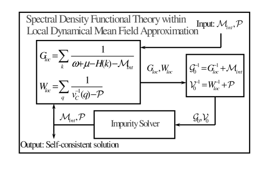
Figure 10: Illustration of the self–consistent cycle in spectral density functional theory within the local dynamical mean–field approximation: both local Green’s function $G_{loc}$ and local Coulomb interaction $W_{loc}$ are iterated. Here we illustrate one possible explicit realization of the abstract general SDFT construction. This requires an explicit definition of $G_{loc}$, which for the purpose of this figure is done by means of the use of a tight binding basis set.

An interesting observation can be made on the role of the impurity model which in the present context appeared as an approximate way to extract the self–energy of the lattice using input bath Green’s function and bath interaction. Alternatively, the impurity problem can be thought of itself as the model which delivers the exact mass operator of the spectral density functional Chitra and Kotliar (2001). If the latter is known, there should exist a bath Green’s function and a bath interaction which can be used to reproduce it. In this respect, the local interaction $W_{loc}$ appearing in our formulation can be thought of as an exact way to define the local Coulomb repulsion “$U$”, i.e. the interaction which delivers exact local self–energy.

$\bullet$ Local GW. A simplified version of the described construction Kotliar and Savrasov (2001); Zein and Antropov (2002) is known as a local version of the GW method (LGW). Within the spectral density functional theory, this approximation appears as an approximation to the functional $\Psi_{SDFT}[G_{loc},W_{loc}]$ taken in the form

$$\Psi_{LGW}[G_{loc},W_{loc}]=-\frac{1}{2}\mathrm{Tr}G_{loc}W_{loc}G_{loc}.$$ (151)

As a result, the susceptibility $\mathcal{P}(\mathbf{r},\mathbf{r}^{\prime},i\omega)$ is approximated by the product of two local Green’s functions, i.e. $\mathcal{P}=-2\delta\Psi_{LGW}/\delta W_{loc}=G_{loc}G_{loc},$ and the exchange–correlation part of our mass operator is approximated by the local GW diagram, i.e. $\mathcal{M}_{xc}=\delta\Psi_{LGW}/\delta G_{loc}=-G_{loc}W_{loc}$. Note that since the local GW approximation (151) is relatively cheap from a computational point of view, its implementation for all orbitals within a cluster is feasible. The results of the single–site approximation for the local quantities were already reported in the literature Zein and Antropov (2002).

Note finally that the local GW approximation is just one of the possible impurity solvers to be used in this context. For example, another popular approximation known as the fluctuation exchange approximation (FLEX) Bickers and Scalapino (1989) can be worked out along the same lines.

$\bullet$ Assessment of the method. The described algorithm is quite general, totally ab initio, and allows the determination of various quantities, such as the local one–electron Green’s functions $G_{loc}$ and the dynamically screened local interactions $W_{loc}$. This challenging project so far has only been carried out on the level of a model Hamiltonian Sun and Kotliar (2002). On the other hand, one can view the LDA+DMFT method as an approximate implementation of this program, as discussed in Ref. Savrasov and Kotliar (2004b). Note also that the combination of the DMFT and full GW algorithm has been recently proposed and applied to Ni Biermann et al. (2003). This in principle shows the way to incorporate full $\mathbf{k}$–dependence of the self–energy known diagrammatically within GW. The first implementation of a fully self-consistent spectral density functional calculation within the LDA+DMFT approximation was carried out in Savrasov et al. (2001) using the full potential LMTO basis set (for details see Savrasov and Kotliar (2004a)). Since then the method has been implemented in the exact muffin tin orbital basis set  Chioncel et al. (2003b) as well as in a fully KKR implementation  Minar et al. (2005).

The spectral density functional theory contains the local or cluster GW diagrams together with all higher order local corrections to construct an approximation to the exact $\mathcal{M}_{xc}$. Just like the Kohn–Sham spectra were a good starting point for constructing the quasiparticle spectra for weakly correlated electron systems, we expect that $\mathcal{M}_{xc}$ will be a good approximation for strongly–correlated electron systems. This is a hypothesis that can be checked by carrying out the perturbation expansion in nonlocal corrections.

II.6 Application to lattice dynamics

Computational studies of lattice dynamics and structural stability in strongly–correlated situations is another challenging theoretical problem which has been recently addressed in Refs. Savrasov and Kotliar (2003); Dai et al. (2003). LDA has delivered the full lattice dynamical information and electron–phonon related properties of a variety of simple metals, transition metals, as well as semiconductors with exceptional  accuracy Baroni et al. (2001). This is mainly due to an introduction of a linear response approach Baroni et al. (1987); Zein (1984). This method overcame the problems of traditional techniques based on static susceptibility calculations which generally fail to reproduce lattice dynamical properties of real materials due to difficulties connected with the summations in high–energy states and the inversion of very large dielectric matrix J. T. Devreese and Camp (1983).

Despite these impressive successes, there is by now clear evidence that the present methodology fails when applied to strongly–correlated materials. For example, the local density predictions for such properties as bulk modulus and elastic constants in metallic Plutonium are approximately one order of magnitude off from experiment Bouchet et al. (2000); the phonon spectrum of Mott insulators such as MnO is not predicted correctly by LDA Massidda et al. (1999).

Recently, a linear response method to study the lattice dynamics of correlated materials has been developed Savrasov and Kotliar (2003); Dai et al. (2003). The dynamical matrix being the second order derivative of the energy can be computed using spectral density functional theory. As with the ordinary density functional formulation of the problem Savrasov (1996), we deal with the first order corrections to the charge density, $\delta\rho,$ as well as the first order correction to the Green’s function $\delta\mathcal{G}(i\omega)$ which should be considered as two independent variables in the functional of the dynamical matrix. To find the extremum, a set of the linearized Dyson equations has to be solved self–consistently

$$[-\nabla^{2}+\mathcal{\hat{M}}_{eff}(i\omega)-\epsilon_{\mathbf{k}j\omega}]\delta\psi_{\mathbf{k}j\omega}^{R}+[\delta\mathcal{\hat{M}}_{eff}(i\omega)-\delta\epsilon_{\mathbf{k}j\omega}]\psi_{\mathbf{k}j\omega}^{R}=0,$$ (152)

which leads us to consider the first order changes in the local mass operator $\mathcal{\hat{M}}_{eff}(i\omega).$ Here and in the following we will assume that the phonon wave vector of the perturbation $\mathbf{q}$ is different from zero, and, therefore, the first order changes in the eigenvalues $\delta\epsilon_{\mathbf{k}j\omega}$ drop out. The quantity $\delta\mathcal{\hat{M}}_{eff}(i\omega)$ is a functional of $\delta\mathcal{G}(i\omega)$ and should be found self–consistently. In particular, the change in the self–energy $\delta\mathcal{\hat{M}}_{eff}(i\omega)$ needs a solution of an AIM linearized with respect to the atomic displacement, which in practice requires the computation of a two-particle vertex function $\Gamma=\delta^{2}\Phi_{SDFT}(G_{loc})/(\delta G_{loc}\delta G_{loc})$.

In practice, change in the eigenvector $\delta\psi_{\mathbf{k}j\omega}$ has to be expanded in some basis set. Previous linear response schemes were based on tight–binding methods Varma and Weber (1977), plane wave pseudopotentials Baroni et al. (1987); Zein (1984); Gonze et al. (1992); Quong and Klein (1992), linear augmented plane wavesYu and Krakauer (1994), mixed orbitals Heid and Bohnen (1999) and linear muffin–tin orbitals Savrasov (1992). Due to explicit dependence on the atomic positions of local orbital basis sets both Hellmann–Feynman contributions and incomplete basis set corrections appear in the expression for the dynamical matrix Savrasov (1996). The functions $\delta\psi_{\mathbf{k}j\omega}$ are represented as follows

$$\delta\psi_{\mathbf{k}j\omega}=\sum_{\alpha}\{\delta A_{\alpha}^{\mathbf{k}j\omega}\chi_{\alpha}^{\mathbf{k+q}}+A_{\alpha}^{\mathbf{k}j\omega}\delta\chi_{\alpha}^{\mathbf{k}}\},$$ (153)

where we introduced both changes in the frequency–dependent variational coefficients $\delta A_{\alpha}^{\mathbf{k}j\omega}$ as well as changes in the basis functions $\delta\chi_{\alpha}^{\mathbf{k}}.$ The latter helps us to reach fast convergence in the entire expression (153) with respect to the number of the basis functions {$\alpha\}$ since the contribution with $\delta\chi_{\alpha}^{\mathbf{k}}$ takes into account all rigid movements of the localized orbitals Savrasov (1992).

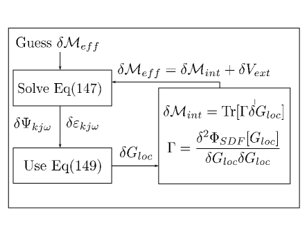
Figure 11: Illustration of the self–consistent cycle to calculate lattice dynamics within the spectral density functional theory.

The first–order changes in the Green’s function can be found as follows

$$\delta G_{loc}(i\omega)=\sum_{\mathbf{k}j}\frac{\delta\psi_{\mathbf{k}j\omega}^{L}\psi_{\mathbf{k}j\omega}^{R}+\psi_{\mathbf{k}j\omega}^{L}\delta\psi_{\mathbf{k}j\omega}^{R}}{i\omega+\mu-\epsilon_{\mathbf{k}j\omega}},$$ (154)

which should be used to evaluate the first order change in the charge density and the dynamical matrix itself (see Fig. 11).

A simplified version of the approach, neglecting the impurity vertex function, was successfully applied to the paramagnetic phases of Mott insulators Savrasov and Kotliar (2003) as well as to high–temperature phases of Plutonium Dai et al. (2003). We will describe these applications in Section IV.

II.7 Application to optics and transport

Optical spectral functions such as conductivity or reflectivity are very important characteristics of solids and give us a direct probe of the electronic structure.

Here we outline an approach which allows to calculate the optical properties of a strongly–correlated material within the spectral density functional framework Oudovenko et al. (2004b); Perlov et al. (2004). This work extends the methodology in use for weak correlated systems (see Maksimov et al. (1988)) to correlated materials. The optical conductivity can be expressed via equilibrium state current–current correlation function Mahan (1993) and is given by

$$\sigma_{\mu\nu}(\omega)=$$ (155)

$$\pi e^{2}\int\limits_{-\infty}^{+\infty}d\varepsilon\phi_{\mu\nu}(\varepsilon+\omega/2,\varepsilon-\omega/2)\frac{f(\varepsilon-\omega/2{)-}f(\varepsilon+\omega/2{)}}{\omega},$$

where $f(\varepsilon)$ is the Fermi function, and the transport function $\phi_{\mu\nu}(\varepsilon,\varepsilon^{\prime})$ is

$$\phi_{\mu\nu}(\varepsilon,\varepsilon^{\prime})=\frac{1}{\Omega_{c}}\sum\limits_{\mathbf{k}jj^{\prime}}\mathrm{Tr}\left\{\nabla_{\mu}\rho_{\mathbf{k}j}{(\varepsilon)\nabla_{\nu}}\rho_{\mathbf{k}j^{\prime}}{(\varepsilon}^{\prime}{)}\right\},$$ (156)

where $\Omega_{c}$ is the unit cell volume and

$$\hat{\rho}_{\mathbf{k}j}(\varepsilon)=-\frac{1}{2\pi i}\left(\mathcal{G}_{\mathbf{k}j}(\varepsilon)-\mathcal{G}_{\mathbf{k}j}^{\dagger}(\varepsilon)\right),$$ (157)

is expressed via retarded one–particle Green’s function, $\mathcal{G}_{\mathbf{k}j}(\varepsilon)$, of the system. Taking limit of zero temperature and using the solutions $\epsilon_{\mathbf{k}j\omega}$ and $\psi_{\mathbf{k}j\omega}^{R,L}$ of the Dyson equation (144), (145) on the real frequency axis we express the optical conductivity in the form

$$\sigma_{\mu\nu}(\omega)={\pi e^{2}\over\omega}\sum_{ss^{\prime}=\pm}ss^{\prime}\sum_{\mathbf{k}jj^{\prime}}\int\limits_{-\omega/2}^{+\omega/2}d\varepsilon\frac{M_{\mathbf{k}jj^{\prime}}^{ss^{\prime},\mu\nu}(\varepsilon^{-},\varepsilon^{+})}{\omega+\epsilon_{\mathbf{k}j\varepsilon^{-}}^{s}-\epsilon_{\mathbf{k}j^{\prime}\varepsilon^{+}}^{s^{\prime}}}\left[\frac{1}{\varepsilon^{-}+\mu-\epsilon_{\mathbf{k}j\varepsilon^{-}}^{s}}{-}\frac{1}{\varepsilon^{+}+\mu-\epsilon_{\mathbf{k}j^{\prime}\varepsilon^{+}}^{s^{\prime}}}\right],$$ (158)

where we have denoted $\varepsilon^{\pm}=\varepsilon\pm\omega/2$, and used the abbreviated notations $\epsilon_{\mathbf{k}j\varepsilon}^{+}\equiv\epsilon_{\mathbf{k}j\varepsilon}$, $\epsilon_{\mathbf{k}j\varepsilon}^{-}=\epsilon_{\mathbf{k}j\varepsilon}^{\ast}$.

The matrix elements $M_{\mathbf{k}jj^{\prime}}$ are generalizations of the standard dipole allowed transition probabilities which are now defined with the right and left solutions $\psi^{R}$and $\psi^{L}$ of the Dyson equation

$$M_{\mathbf{k}jj^{\prime}}^{ss^{\prime},\mu\nu}(\varepsilon,\varepsilon^{\prime})=$$ (159)

$$\int(\psi_{\mathbf{k}j\varepsilon}^{s})^{s}\nabla_{\mu}(\psi_{\mathbf{k}j\varepsilon^{\prime}}^{-s^{\prime}})^{s^{\prime}}d\mathbf{r}\int(\psi_{\mathbf{k}j^{\prime}\varepsilon^{\prime}}^{s^{\prime}})^{s^{\prime}}\nabla_{\nu}(\psi_{\mathbf{k}j\varepsilon}^{-s})^{s}d\mathbf{r},$$

where we have denoted $\psi_{\mathbf{k}j\varepsilon}^{+}=\psi_{\mathbf{k}j\varepsilon}^{L}$ , $\psi_{\mathbf{k}j\varepsilon}^{-}=\psi_{\mathbf{k}j\varepsilon}^{R}$ and assumed that $(\psi_{\mathbf{k}j\varepsilon}^{s})^{+}\equiv\psi_{\mathbf{k}j\varepsilon}^{s}$ while $(\psi_{\mathbf{k}j\varepsilon}^{s})^{-}=\psi_{\mathbf{k}j\varepsilon}^{s\ast}$. The expressions (158), (II.7) represent generalizations of the formulae for optical conductivity for a strongly–correlated system, and involve the extra internal frequency integral in Eq. (158).

Let us consider the non–interacting limit when $\mathcal{\hat{M}}_{xc}(\omega)\rightarrow i\gamma\rightarrow 0.$ In this case, the eigenvalues $\epsilon_{\mathbf{k}j\varepsilon}=\epsilon_{\mathbf{k}j}+i\gamma,\psi_{\mathbf{k}j\varepsilon}^{R}\equiv|\mathbf{k}j\rangle,$ $\psi_{\mathbf{k}j\varepsilon}^{L}\equiv|\mathbf{k}j\rangle^{\ast}\equiv\langle\mathbf{k}j|$ and the matrix elements $M_{\mathbf{k}jj^{\prime}}^{ss^{\prime},\mu\nu}(\varepsilon,\varepsilon^{\prime})$ are all expressed via the standard dipole transitions $|\langle\mathbf{k}j|\nabla|\mathbf{k}j^{\prime}\rangle|^{2}.$ Working out the energy denominators in the expression (158) in the limit $i\gamma\rightarrow 0$ and for $\omega\neq 0$ leads us to the usual form for the conductivity which for its interband contribution has the form

$$\sigma_{\mu\nu}(\omega) = \frac{\pi e^{2}}{\omega}\sum_{\mathbf{k},j^{\prime}\neq j}\langle\mathbf{k}j|\nabla_{\mu}|\mathbf{k}j^{\prime}\rangle\langle\mathbf{k}j^{\prime}|\nabla_{\nu}|\mathbf{k}j\rangle\times$$ (160)

$$[f(\epsilon_{\mathbf{k}j})-f(\epsilon_{\mathbf{k}j^{\prime}})]\delta(\epsilon_{\mathbf{k}j}-\epsilon_{\mathbf{k}j^{\prime}}+\omega).$$

To evaluate the expression $\sigma_{\mu\nu}(\omega)$ numerically, one needs to pay special attention to the energy denominator $1/(\omega+\epsilon_{\mathbf{k}j\varepsilon^{-}}^{s}-\epsilon_{\mathbf{k}j^{\prime}\varepsilon^{+}}^{s^{\prime}})$ in (158). Due to its strong $\mathbf{k}$-dependence the tetrahedron method of Lambin and Vigneron Lambin and Vigneron (1984) should be used. On the other hand, the difference in the square brackets of Eq. (158) is a smooth function of $\mathbf{k}$ and one can evaluate it using linear interpolation. This allows one to calculate the integral over $\varepsilon$ by dividing the interval $-\omega/2<\varepsilon<+\omega/2$ into discrete set of points $\varepsilon_{i}$ and assuming that the eigenvalues $\epsilon_{\mathbf{k}j\varepsilon}$ and eigenvectors $\psi_{\mathbf{k}j\varepsilon}$ can to zeroth order be approximated by their values at the middle between each pair of points i.e. $\bar{\varepsilon}_{i}^{\pm}=\varepsilon_{i}\pm\omega/2+(\varepsilon_{i+1}-\varepsilon_{i})/2$. In this way, the integral is replaced by the discrete sum over internal grid $\varepsilon_{i}$ defined for each frequency $\omega,$ and the Dyson equation needs to be solved twice for the energy $\bar{\varepsilon}_{i}^{+}$ and for the energy $\bar{\varepsilon}_{i}^{-}$ The described procedure produces fast and accurate algorithm for evaluating the optical response functions of a strongly–correlated material.

Similar developments can be applied to calculate the transport properties such as $dc$-resistivity. The transport parameters of the system are expressed in terms of so called kinetic coefficient, denoted here by $A_{m}$. The equation for the electrical resistivity is given by

$$\rho=\frac{k_{B}T}{e^{2}}\frac{1}{A_{0}},$$ (161)

and the thermopower and the thermal conductivity are given by

$$S=\frac{-k_{B}}{|e|}\frac{A_{1}}{A_{0}},\qquad\kappa=k_{B}\left(A_{2}-\frac{A_{1}^{2}}{A_{0}}\right).$$ (162)

Within the Kubo formalism Mahan (1993) the kinetic coefficients are given in terms of equilibrium state current–current correlation functions of the particle and the heat current in the system. To evaluate these correlation functions an expression for electric and heat currents are needed. Once those currents are evaluated, transport with DMFT reduces to the evaluation of the transport function

$$\phi^{xx}(\epsilon)=\frac{1}{\Omega_{c}}\sum_{k}\mbox{Tr}\left\{\hat{v}^{x}_{k}(\epsilon)\hat{\rho}_{k}(\epsilon)\hat{v}^{x}_{k}(\epsilon)\hat{\rho}_{k}(\epsilon)\right\},$$ (163)

and the transport coefficients

$$A_{m}=\pi\int_{-\infty}^{\infty}d\epsilon\phi^{xx}(\epsilon)f(\epsilon)f(-\epsilon)(\beta\epsilon)^{m},$$ (164)

The described methodology has been applied to calculate the optical conductivity Oudovenko et al. (2004b), the thermopower Pálsson and Kotliar (1998), the DC–resistivity, and the thermal conductivity for LaTiO₃ Oudovenko et al. (2004c).

III Techniques for solving the impurity model

In practice the solution of the dynamical mean–field (DMFT) equations is more involved than the solution of the Kohn–Sham equations, which now appear as static analogs. There are two central elements in DMFT: the self–consistency condition and the impurity problem (see Fig. 5). The first step is trivial for model calculations but becomes time consuming when realistic band structures are considered. Usually it is done using the tetrahedron method (see, e.g., Anisimov et al. (1997a), programs and algorithms for caring out this step are described at $http://dmftreview.rutgers.edu$).

The second step in the DMFT algorithm, i.e. the solution of the impurity problem, is normally the most difficult task. Fortunately, we can now rely on many years of experience to devise reasonable approximations for carrying out this step. At the present time, there is no universal impurity solver that works efficiently and produces accurate solutions for the Green’s function in all regimes of parameters. Instead what we have is a large number of techniques, which are good in some regions of parameters. In many cases when there are various methods that can be applied, there is a conflict between accuracy and computational cost, and in many instances one has to make a compromise between efficiency and accuracy to carry out the exploration of new complex materials. It should be noted that the impurity solver is one component of the various algorithms discussed, and that for a given material or series of materials, one should strive to use comparable realism and accuracy in the various stages of the solution of a specific problem.

For space limitations, we have not covered all the methods that are available for studying impurity models, but we simply chose a few illustrative methods which have been useful in the study of correlated materials using DMFT. In this introductory section, we give an overview of some of the methods, pointing out the strengths and limitations of them and we expand on the technical details in the following subsections.

There are two exactly soluble limits of the multiorbital Anderson impurity model, for a general bath. The atomic limit when the hybridization vanishes and the band limit when the interaction matrix $U$ is zero. There are methods which are tied to expansions around each of these limits. The perturbative expansion in the interactions is described in section III.1. It is straightforward to construct the perturbative expansion of the self–energy in powers of $U$ up to second order, and resum certain classes of diagrams such as ring diagrams and ladder diagrams. This is an approach known as the fluctuation exchange approximation (FLEX), and it is certainly reliable when $U$ is less than the half–bandwidth, $D$. These impurity solvers are very fast since they only involve matrix multiplications and inversions. They also have good scaling, going as $N^{3}$ where $N$ is the number of orbitals or the cluster size.

The expansion around the atomic limit is more complicated. A hybridization function with spectral weight at low frequencies is a singular perturbation at zero temperature. Nevertheless approaches based on expansion around the atomic limit are suitable for describing materials where there is a gap in the one–particle spectra, or when the temperature is sufficiently high that one can neglect the Kondo effect. This includes Mott insulating states at finite temperatures, and the incoherent regime of many transition metal oxides and heavy fermion systems. Many approaches that go beyond the atomic limit exist: direct perturbation theory in the hybridization, resummations based on equation of motion methods, such as the Hubbard approximations, resolvent methods, and slave particle techniques such as the non–crossing approximation (NCA) and their extensions. We describe them in sections III.2 and III.3.

There are methods, such as the quantum Monte Carlo method (QMC), or functional integral methods which are not perturbative in either $U$ or in the bandwidth, $W$. In the QMC method one introduces a Hubbard–Stratonovich field and averages over this field using Monte Carlo sampling. This is a controlled approximation using a different expansion parameter, the size of the mesh for the imaginary time discretization. Unfortunately, it is computationally very expensive as the number of time slices and the number of Hubbard–Stratonovich fields increases. The QMC method is described in section III.4. It also has a poor scaling with the orbital degeneracy, since the number of Hubbard–Stratonovich fields increases as the square of the orbital degeneracy. Mean–field methods are based on a functional integral representation of the partition function, and the introduction of auxiliary slave bosons Barnes (1976, 1977); Coleman (1984). The saddle point approximation Kotliar and Ruckenstein (1986); Rasul and Li (1988) gives results which are very similar to those of the Gutzwiller method, and corrections to the saddle point can be carried out by a loop expansion Li et al. (1989). Unfortunately the perturbative corrections to the saddle point are complicated and have not been evaluated in many cases. We review the mean–field theory in section III.5.

Interpolative methods bear some resemblance to the analytic parameterizations of $V_{xc}$ in LDA. One uses different approximations to the self–energy of the impurity model, viewed as a functional of $\Delta(i\omega)$, in different regions of frequency. The idea is to construct interpolative formulae that become exact in various limits, such as zero frequency where the value of the Green’s function is dictated by Luttinger theorem, high frequencies where the limiting behavior is controlled by some low–order moments, and in weak and strong coupling limits where one can apply some form of perturbation theory. This approach has been very successful in unraveling the Mott transition problem in the context of model Hamiltonians, and it is beginning to be used for more realistic studies. We review some of these ideas in section III.6.

In this review, we have not covered techniques based on exact diagonalization methods, and their improvements such as Wilson renormalization group (RG) techniques and density matrix renormalization group methods. These are very powerful techniques, but due to the exponential growth of the Hilbert space, they need to be tailored to the application at hand. In the context of model Hamiltonians, it is worth mentioning that the exact solution for the critical properties of the Mott transition was obtained with the projective self–consistent method Moeller et al. (1995), which is an adaptation of Wilson RG ideas to the specifics of the DMFT study of the Mott transition. This method sets up a Landau theory and justifies the use of exact diagonalization for small systems to determine the critical properties near the transition. Further simplifications of these ideas, which in practice amounts to the exact diagonalization methods with one site, have been used by Potthoff and coworkers Potthoff (2001). The flow equation method of Wilson and Glazek and Wegner Glazek and Wilson (1993, 1994); Wegner (1994) is another adaptive technique for diagonalizing large systems, and it has been applied to the impurity model. Clearly, the renormalization group approach in the cluster DMFT context is necessary to attack complex problems. Some ideas for combining cellular DMFT with RG formalism were put forward in the context of model Hamiltonians Bolech et al. (2003).

Finally, we point out that a much insight is gained when numerical methods are combined with analytic studies. As in the previous applications of DMFT to model Hamiltonians, fast approximate techniques and algorithms are needed to make progress in the exploration of complex problems, but they should be used with care and tested with more exact methods.

III.1 Perturbation expansion in Coulomb interaction

The application of perturbation theory in the interaction $U$ has a long history in many–body theory. For DMFT applications, we consider here a general multiorbital Anderson impurity model (AIM) given by

$$H = \sum_{\alpha\beta}\epsilon_{\alpha\beta}d_{\alpha}^{\dagger}d_{\beta}+\frac{1}{2}\sum_{\alpha\beta\gamma\delta}U_{\alpha\beta\gamma\delta}d_{\alpha}^{\dagger}d_{\beta}^{\dagger}d_{\gamma}d_{\delta}$$

$$+ \sum_{k\alpha\beta}(V_{k\alpha\beta}^{*}d^{\dagger}_{\alpha}c_{k\beta}+H.c.)+\sum_{k\alpha}\epsilon_{k\alpha}c^{\dagger}_{k\alpha}c_{k\alpha},$$

where $U_{\alpha\beta\gamma\delta}$ is the most general interaction matrix and $\alpha$ combines spin and orbital index (or position of an atom in the unit cell or cluster, in cellular DMFT applications).

The lowest order term is the Hartree–Fock formulae

$$\Sigma_{12}^{(HF)}=\sum_{34}(U_{1342}-U_{1324})n_{43}.$$ (166)

The second order term is given by

$$\Sigma_{12}^{(2)}(i\omega)=\sum_{\{3-8\}}U_{1456}U_{7832}\int\int\int d\epsilon d\epsilon^{\prime}d\epsilon^{\prime\prime}\rho_{67}(\epsilon)\rho_{58}(\epsilon^{\prime})\rho_{34}(\epsilon^{\prime\prime}){\frac{{f(\epsilon)f(\epsilon^{\prime})f(-\epsilon^{\prime\prime})+f(-\epsilon)f(-\epsilon^{\prime})f(\epsilon^{\prime\prime})}}{i\omega-\epsilon+\epsilon^{\prime\prime}-\epsilon^{\prime}}},$$ (167)

where $f$ is the Fermi function, ${\rho}_{12}$ is the spectral function of the impurity Green’s function.

Figure 12: Particle–particle (top row) and particle–hole (bottom row) $T$–matrices which appear in the FLEX approximation. Full lines correspond to electron propagators and wiggly lines stand for the bare interaction $U$.

Figure 13: Definition of the FLEX self–energy constructed with the help of particle–particle and particle–hole $T$–matrices. Note that some lower order terms appear many times and need to be subtracted to avoid double counting.

Higher order terms in perturbation theory that can be easily summed up are those in the form of a ladder or, equivalently, $T$–matrix. There are two distinct types of ladder graphs, the particle–particle type Galitskii (1958) shown in the top row of Fig. 12 and particle–hole $T$–matrix depicted in the bottom row of Fig. 12. The one–particle self–energy can then be constructed using those two building blocks in the way shown in Fig. 13. Although we did not plot the generating functional, which in the general case is somewhat more involved, it can be constructed order by order from the above definition of the self–energy. Hence, the approximation is conserving if the propagators are fully dressed, and therefore automatically obeys certain microscopic conservation laws as well as the Friedel sum rule. The method was first proposed by Bickers and Scalapino in the context of lattice models Bickers and Scalapino (1989) under the name fluctuation exchange approximation (FLEX). It is the minimal set of graphs describing the interaction of quasiparticles with collective modes (pairs, spin and charge fluctuations).

Particle–particle and particle–hole $T$–matrices correspond algebraically to

$$\hat{T}^{pp}(i\Omega) = (1-\hat{U}\hat{\chi}^{pp}_{i\Omega})^{-1}\hat{U}\hat{\chi}^{pp}_{i\Omega}\hat{U}\hat{\chi}^{pp}_{i\Omega}\hat{U},$$ (168)

$$\hat{T}^{ph}(i\Omega) = (1-(\hat{V}+\hat{W})\hat{\chi}^{ph}_{i\Omega})^{-1}(\hat{V}+\hat{W})$$ (169)

$$- (\hat{V}+\hat{W})\hat{\chi}^{ph}_{i\Omega}\hat{V},$$

where $V_{1234}=U_{1324}$, $W_{1234}=-U_{1342}$ and

$$\chi_{1234}^{pp}(i\Omega)=-T\sum_{i\omega^{\prime}}G_{23}(i\omega^{\prime})G_{14}(i\Omega-i\omega^{\prime}),$$ (170)

$$\chi_{1234}^{ph}(i\Omega)=-T\sum_{i\omega^{\prime}}G_{23}(i\omega^{\prime})G_{41}(i\Omega+i\omega^{\prime}).$$ (171)

We assumed here a product of the form $(\hat{A}\hat{B})_{1234}=\sum_{56}A_{1256}B_{5634}$. With these building blocks one can construct the self–energy of the form

$$\Sigma_{12}^{(FLEX)}(i\omega)=T\sum_{i\Omega 34}\left(T^{pp}_{1432}(i\Omega)G_{34}(i\Omega-i\omega)\right.$$

$$+\left.T^{ph}_{1432}(i\Omega)G_{43}(i\Omega+i\omega)\right).$$ (172)

The Feynman graphs in perturbation theory can be evaluated self–consistently (namely in terms of fully dressed Green’s function, $G$, including only skeleton graphs) or non–self–consistently (namely using $G_{0}$). In practice the results start being different once $U$ is comparable to the half bandwidth. The skeleton perturbation theory in $G$ sums more graphs than the bare perturbation theory, but in many–body theory more does not necessarily imply better. In the context of the single–band AIM model, the perturbative approach in powers of the Hartree–Fock Green’s function $G_{0}$ was pioneered by Yamada and Yoshida Yosida and Yamada (1970); Yamada (1975); Yosida and Yamada (1975a, b). These ideas were crucial for the first implementation of DMFT Georges (1992) for the one–band Hubbard model, where the expansion in $G_{0}$ proved to be qualitatively and quantitatively superior to the expansion in $G$. In the multiorbital case, the situation is far less clear as discussed recently in Ref. Drchal et al., 2005.

Figure 14: Particle hole $T_{ph}$ ladder contribution with screened effective interaction $U_{eff}$ mediated by $T_{pp}$.

Bulut and Scalapino Bulut et al. (1993), tested Kanamori’s Kanamori (1963) observation that the particle–hole bubbles should interact not with the bare interaction matrix, $U$ in Eq. 169, but with an effective interaction screened by the particle–particle ladder (see Fig 14). This can be approximated by replacing $U$ by $U_{eff}=T_{pp}(\omega=0)$ in Eq. 169. Notice that those diagrams are a subset of the parquet graphs, recently implemented by Bickers Bickers and White (1991). It is also worth noticing that the FLEX approach is exact to order $U^{3}$.

Within the realistic DMFT, the FLEX method was implemented for Iron and Nickel (in its non–self–consistent form) by Drchal et al. Drchal et al. (1999) and Katsnelson et al. Chioncel et al. (2003c) (these authors used the expansion in $G_{0}$ where an additional shift of the impurity level is implemented to satisfy Luttinger’s theorem following Ref. Kajueter and Kotliar, 1996b, and the screened interaction in the particle–hole channel was assumed).

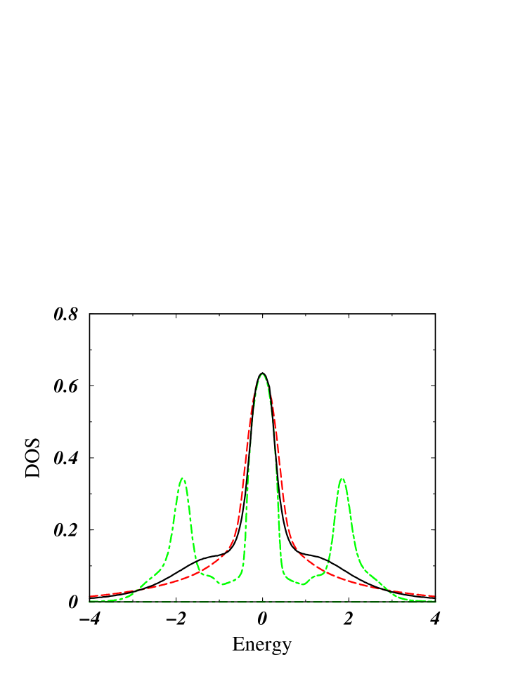
Figure 15: Comparison of FLEX density of states (using $T_{pp}$ graphs only) with QMC results (full line). Dashed line corresponds to FLEX approximation with fully dressed propagators and dashed–dotted line stands for the same approximation with undressed propagators. Calculation was performed for a two–band Hubbard model for semicircular density of states with $U=2D$ and $T=1/16D$ Drchal et al. (2005).

When the interaction is much less than the half–bandwidth the perturbative corrections are small and all the approaches (self–consistent, non–self–consistent, screened or unscreened) are equivalent to the second order graph. However, when $U$ becomes comparable to the half bandwidth differences appear, and we highlight some qualitative insights gained from a comparison of the various methods Drchal et al. (2005); Putz et al. (1996). The perturbation theory in $G_{0}$ tends to overestimate $Z^{-1}$ and overemphasize the weight of the satellites. On the other hand the skeleton perturbation theory tends to underestimate the effects of the correlations and suppress the satellites. This is clearly seen in Fig. 15 where perturbative results are compared to QMC data, analytically continued to real axis with the maximum entropy method (MEM) Jarrell and Gubernatis (1996).

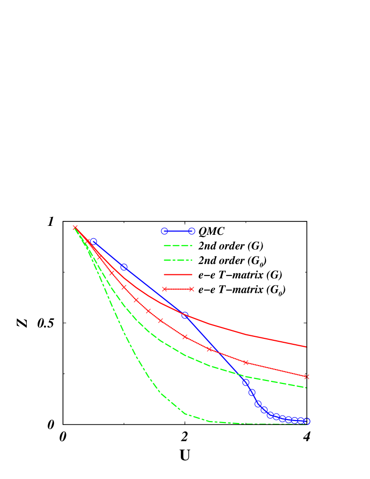
Figure 16: Variation of quasiparticle residue with interaction strength of the interaction for two–band half–filled Hubbard model with a semicircular density of states of bandwidth $D$. Schemes presented are: second order perturbation with fully dressed propagators(dashed curve), second order with Hartree–Fock dressing of propagators (dot–dashed), FLEX with electron–electron $T$–matrix only but fully self–consistent (solid line), FLEX with electron–electron $T$–matrix only and Hartree–Fock dressing of propagators (line with stars) Drchal et al. (2005).

To gauge the region in which the approach is applicable, we compare the quasiparticle weight from various perturbative approaches to QMC data in Fig. 16. All self–consistent approaches miss the existence of the Mott transition, while its presence or at least a clear hint of its existence appears in the second order non–self–consistent approach.

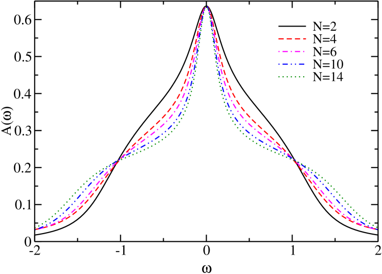
Figure 17: Variation of FLEX spectra with increasing number of bands for $U=D$ and $T=0.001$ on the Bethe lattice. The self–consistency is obtained by fully dressed propagators including all three FLEX channels Drchal et al. (2005).

While FLEX performs reasonably well in the case of two- and three–band models, it is important to stress that this can not persist to very large degeneracy. With increasing number of bands, the quasiparticle residue must increase due to enhancement of screening effect and therefore $Z$ must grow and eventually approach unity. This remarkable screening effect is not captured by FLEX which displays the opposite trend as shown in Fig. 17.

It is worth noticing that for Ni the full $d$–bandwidth is approximately 4.5 eV and $U$ is estimated to be around 3 eV so the approach is near the boundary of its applicability.

III.2 Perturbation expansion in the hybridization strength

The perturbation expansion with respect to the hybridization strength can be derived with the help of resolvent techniques or by decoupling of Hubbard operators in terms of slave particles. In the latter case, an auxiliary operator $a_{n}$ is assigned to each state of the local Hilbert space, such that a slave particle creates an atomic state out of the new vacuum

$$\left|n\right>=a_{n}^{\dagger}\left|vac\right>,$$ (173)

where $\left|vac\right>$ is a new vacuum state. The Hubbard operators are easily expressed in terms of this auxiliary particles, $X_{n,m}=a_{n}^{\dagger}a_{m}$. The creation operator of an electron is expressed by

$$d^{\dagger}_{\alpha}=\sum_{nm}(F^{\alpha\dagger})_{nm}a_{n}^{\dagger}a_{m},$$ (174)

where $F_{nm}^{\alpha}=\langle n|d_{\alpha}|m\rangle$ are matrix elements of a destruction operator. In terms of pseudo particles, the general Anderson impurity model reads

$$H=\sum_{mn}E_{mn}a_{n}^{\dagger}a_{m}+\sum_{k\gamma}\varepsilon_{k\gamma}c_{k\gamma}^{\dagger}c_{k\gamma}+$$

$$\sum_{k,mn,\alpha\beta}\left(V^{*}_{k\alpha\beta}(F^{\alpha\dagger})_{nm}a_{n}^{\dagger}a_{m}c_{k\beta}+H.c.\right),$$ (175)

where $c_{k\gamma}^{\dagger}$ creates an electron in the bath and $\gamma$ stands for the spin and band index.

In order that electrons are faithfully represented by the auxiliary particles, i.e. $\{d_{\alpha},d_{\beta}^{\dagger}\}=\delta_{\alpha\beta}$, the auxiliary particle $a_{n}$ must be boson (fermion), if the state $\left|n\right>$ contains even (odd) number of electrons, and the constraint:

$$Q\equiv\sum_{n}a_{n}^{\dagger}a_{n}=1,$$ (176)

must be imposed at all times. This condition merely expresses the completeness relation for the local states $\sum_{n}\left|n\right>\left<n\right|=1$. The constraint is imposed by adding a Lagrange multiplier $\lambda Q$ to the Hamiltonian and the limit $\lambda\rightarrow\infty$ is carried out.

The physical local Green’s function (electron Green’s function in $Q=1$ subspace) and other observables are calculated with the help of the Abrikosov trick Abrikosov (1965) which states that the average of any local operator that vanishes in the $Q=0$ subspace is proportional to the grand–canonical (all $Q$ values allowed) average of the same operator

$$\langle A\rangle_{Q=1}=\lim_{\lambda\rightarrow\infty}{\frac{\langle A\rangle_{G}}{\langle Q\rangle_{G}}}.$$ (177)

The advantage of pseudo–particle approach is that standard diagrammatic perturbation theory techniques such as Wicks theorem can be applied. The limit $\lambda\rightarrow\infty$ is to be taken after the analytic continuation to the real frequency axes is performed. Taking this limit, actually leads to a substantial simplification of the analytic continuation Haule et al. (2001).

A different approach, is to “soften” the constraint $Q=1$, and replace it by

$$\sum_{n}a^{\dagger}_{n}a_{n}=q_{0}N.$$ (178)

The original problem corresponds to taking $q_{0}=1/N$ but one can obtain a saddle point by keeping $q_{0}$ of order of one while allowing $Q$ to be large. This approach, was studied in Ref. Parcollet and Georges (1997); Parcollet et al. (1998). While the standard NCA approach suffers from exceeding the unitary limit leading to causality problems, the soft NCA’s do not suffer from that problem. Other sub–unitary impurity solvers were developed recently based on slave rotor methods Florens and Georges (2002, 2004) and on a decoupling schemes Costi (1986); Jeschke and Kotliar (2005).

The perturbation expansion in the hybridization strength can be easily carried out in the pseudo–particle representation. The desired quantity of the expansion is the local Green’s function which is proportional bath electron $T$–matrix, therefore we have

$$G_{loc}=\lim_{\lambda\rightarrow\infty}{\frac{1}{V^{2}\langle Q\rangle_{G}}}\Sigma_{c},$$ (179)

where $\Sigma_{c}$ is the bath electron self–energy calculated in the grand–canonical ensemble. The latter quantity has a simple diagrammatic interpretation.

Figure 18: Diagrammatic representation of the non–crossing approximation (NCA) and one–crossing approximation (OCA) functional for the Anderson impurity model.

The selection of diagrams, is best illustrated using the Baym–Kadanoff functional $\Phi$. The building blocks of $\Phi$ are dressed Green’s functions of pseudo–particles $G_{mn}$ (depicted as dashed lines), and bath electrons $G_{\alpha\beta}$ (solid lines). Due to the exact projection, only pseudo–particles are fully dressed while bath electron Green’s functions are non–dressed because the bath self–energy vanishes as $exp(-\beta\lambda)$ with $\lambda\rightarrow\infty$. The bare vertex $V_{k\alpha\beta}$, when combined with the conduction electron propagator, can be expressed in terms of the bath spectral function $A_{\alpha\beta}(\omega)=-{1\over 2\pi i}[\Delta_{\alpha\beta}(\omega+i0^{+})-\Delta_{\alpha\beta}(\omega-i0^{+})]$. Because propagators are fully dressed, only skeleton diagrams need to be considered in the expansion.

The lowest order contribution, depicted in the first line of Fig. 18 is known in literature as non–crossing approximation (NCA). Pseudo–particle self–energies $\Sigma_{mn}$, defined through $(G^{-1})_{mn}=(\omega-\lambda)\delta_{mn}-E_{mn}-\Sigma_{mn}$, are obtained by taking the functional derivative of $\Phi$ with respect to the corresponding Green’s function, i.e. $\Sigma_{mn}=\delta\Phi/\delta G_{nm}$. After analytic continuation and exact projection, the self–energies obey the following coupled equations

$$\Sigma_{mn}(\omega+i0^{+}) = \sum_{\alpha\beta,m^{\prime}n^{\prime}}\left[F^{\beta}_{mm^{\prime}}(F^{\alpha\dagger})_{n^{\prime}n}\int d\xi f(\xi)A_{\alpha\beta}(\xi)G_{m^{\prime}n^{\prime}}(\omega+\xi+i0^{+})\right.$$ (180)

$$\left.\qquad+(F^{\beta\dagger})_{mm^{\prime}}F^{\alpha}_{n^{\prime}n}\int d\xi f(-\xi)A_{\beta\alpha}(\xi)G_{m^{\prime}n^{\prime}}(\omega-\xi+i0^{+})\right].\ \ \ \ \$$

The local electron Green’s function, obtained by functional derivative of $\Phi$ with respect to the bath Green’s function, becomes

$$G_{\alpha\beta}(\omega+i0^{+})=\sum_{mnm^{\prime}n^{\prime}}F^{\alpha}_{n^{\prime}n}(F^{\beta\dagger})_{mm^{\prime}}{1\over Q}\int d\xi\exp(-\beta\xi)\left[\rho_{m^{\prime}n^{\prime}}(\xi)G_{nm}(\xi+\omega+i0^{+})-G_{m^{\prime}n^{\prime}}(\xi-\omega-i0^{+})\rho_{nm}(\xi)\right],\ \ \ \ \ \$$ (181)

where $A_{\alpha\beta}$ is the bath spectral function defined above, $Q=\int d\xi\exp(-\beta\xi)\sum_{m}\rho_{mm}(\xi)$ is the grand canonical expectation value of charge $Q$ and $\rho_{mn}=-{1\over 2\pi i}[G_{mn}(\omega+i0^{+})-G_{mn}(\omega-i0^{+})]$ is the pseudo–particle density of states. Note that equations are invariant with respect to shift of frequency in the pseudo particle quantities due to local gauge symmetry, therefore $\lambda$ that appears in the definition of the pseudo Green’s functions can be an arbitrary number. In numerical evaluation, one can use this to our advantage and choose zero frequency at the point where the pseudo particle spectral functions diverge.

The NCA has many virtues, it is very simple, it captures the atomic limit, it contains the Kondo energy as a non–perturbative scale and describes the incipient formation of the Kondo resonance. However, it has several pathologies that can be examined analytically by considering the pseudo–particle threshold exponents at zero temperature Müller-Hartmann (1984). Within NCA, the infrared exponents are independent of doping and follow the exact non–Fermi liquid exponents in the multichannel Kondo problem Cox and Ruckenstein (1993). From the Friedel sum rule, however, it follows that fully screened local moment leads to a doping–dependent Fermi liquid exponents that differ substantially from the NCA exponents Costi et al. (1996). When calculating the local spectral function within NCA, this leads to a spurious peak at zero frequency with the Abrikosov–Suhl resonance exceeding the unitary limit. At the temperature at which the Kondo resonance exceeds the unitary limit, the approximation breaks down when combined with DMFT self–consistency conditions, because it causes the spectral function to become negative hence violating causality.

Figure 19: Diagrammatic representation of the two–crossing approximation (TCA) generating functional. It consists of all skeleton diagrams (infinite number) where conduction lines cross at most twice. Conserving $T$–matrix approximation (CTMA) is a subset of diagrams where all conduction lines cross exactly twice and have either clockwise or counter–clockwise direction. Symmetrized U–NCA (SUNCA) is a subset of TCA where a conduction line exists that crosses only once. Conduction lines can have either clockwise or counter–clockwise direction.

At finite $U$, the NCA has a new problem, namely, it severely underestimates the width of the Kondo resonance and hence the Kondo temperature. This problem is partly corrected by the vertex corrections shown in the second row of Fig. 18, which was introduced by Pruschke and Grewe and is called one–crossing approximation (OCA). This diagram is a natural generalization of NCA, namely, including all diagrams with a single line crossing. It is also the lowest order self–consistent approximation exact up to $V^{2}$. Although the pseudo particle self–energies within NCA are calculated up to $V^{2}$, the local Green’s function is not. Only the conduction electron self–energy is exact up to $V^{2}$ and from Eq. (179) it follows that the physical spectral function is not calculated to this order within NCA.

Several attempts were made to circumvent the shortcomings of NCA by summing up certain types of diagrams with ultimate goal to recover the correct infrared exponents and satisfy the unitarity limit given by the Friedel sum rule. It can also be analytically shown, that an infinite resummation of skeleton diagrams is necessary to change the infrared exponents from their NCA values. The natural choice is to consider the ladder type of scatterings between the pseudo–particle and the bath electrons which leads to crossings of conduction lines in the Luttinger–Ward functional. In the infinite $U$ limit, only diagrams where all conduction electrons cross at least twice, are possible. Note that due to the projection, any contribution to the Luttinger–Ward functional consists of a single ring of pseudo–particles since at any moment in time there must be exactly one pseudo–particle in the system. The diagrams where all conduction electrons cross exactly twice is called CTMA Kroha et al. (1997) and has not yet been implemented in the context of the DMFT. A typical contribution to the CTMA Luttinger Ward functional is shown in the second line of Fig. 19. In the impurity context, this approximation recovers correct Fermi liquid infrared exponents in the whole doping range and it is believed to restore Fermi liquid behavior at low temperature and low frequency.

At finite $U$, however, skeleton diagrams with less crossings exist. Namely, a ladder ring where conduction lines cross exactly twice can be closed such that two conduction lines cross only ones. This approximation, depicted in the first row of Fig. 19, is called SUNCA. It has been shown in the context of single impurity calculation Haule et al. (2001), that this approximation further improves the Kondo scale bringing it to the Bethe ansatz value and also restores Fermi liquid exponents in the strict Kondo regime. Unfortunately, this is not enough to restore Friedel sum rule in the local spectral function at low temperatures and to apply the approach to this regime, it has to be combined with other approaches such as renormalized perturbation theory or ideas in the spirit of the interpolative methods discussed in III.6.

The results of the computationally less expensive SUNCA calculation agree very well with the considerably more time consuming QMC calculation. The agreement is especially accurate around the most interesting region of the Mott transition while the half–integer filling shows some discrepancy due to the restriction to a small number of valences in the SUNCA calculation.

Figure 20: Comparison between SUNCA (full line) and QMC (dashed line) density of states for the three–band Hubbard model on the Bethe lattice for $n_{d}=0.8$ at $U=5D$ and $T=D/16$.

We illustrate the agreement between these methods by means of the real axis data of QMC+MEM and SUNCA where the latter results are obtained on the real axis. As shown in Fig. 20, both calculations produce almost identical quasiparticle peak, while some discrepancy can be observed in the shape of Hubbard bands. We believe that this is mostly due to analytic continuation of QMC data which do not contain much high–frequency information. Notice that the width of the upper Hubbard band is correctly obtained within SUNCA while QMC results show redistribution of the weight in much broader region. Namely, in the large $U$ limit, i.e. when a band is separated from the quasiparticle peak, its width has to approach the width of the non–interacting density of states, in this case $2D$.

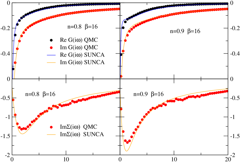
Figure 21: Imaginary axis QMC data (dots) and SUNCA results (full–lines) are compared for three–band Hubbard model on Bethe lattice for $\beta=16$ and $U=5D$. Left panel shows results for doping levels $n_{d}=0.8$ right panel corresponds to doping $n_{d}=0.9$.

Finally, we compare the imaginary axis data in Fig. 21 for two doping levels of $n_{d}=0.8$ and $n_{d}=0.9$. Notice that the results are practically identical with discrepancy smaller that the error of the QMC data.

The NCA was used in the DMFT context to study Cerium Zölfl et al. (2001), ${\rm La}_{1-x}{\rm Sr}_{x}{\rm TiO}_{3}$ Zölfl et al. (2000) and ${\rm Ca}_{2-x}{\rm Sr}_{x}{\rm RuO}_{4}$ Anisimov et al. (2002). In the case of Cerium, it does capture the most essential differences of the alpha and gamma phases, and compares very favorably to the quantum Monte Carlo results Held et al. (2001b) and to experiments. Using NCA in the context of the SrRuO₃, Anisimov et al., 2002 was the first to predict the so-called orbitally selective Mott transition, the phase where one–band is in a Mott insulting state while the rest are metallic. These results are discussed further within (see section IV.1). The SUNCA approach was first tested in the LaSrTiO₃ where it is in a good agreement with QMC results  Oudovenko et al. (2004c).

III.3 Approaching the atomic limit: decoupling scheme, Hubbard I and lowest order perturbation theory

The AIM Hamiltonian can also be expressed in terms of Hubbard operators $X_{nm}$ by replacing $a_{n}^{\dagger}a_{m}$ in Eq. (175) with $X_{nm}$:

$$H=\sum_{m}E_{m}X_{mm}+\sum_{k\gamma}\varepsilon_{k\gamma}c_{k\gamma}^{\dagger}c_{k\gamma}+$$

$$\sum_{k,mn,\alpha\beta}\left(V^{*}_{k\alpha\beta}(F^{\alpha\dagger})_{nm}X_{nm}c_{k\beta}+H.c.\right).$$ (182)

For convenience, we choose here the local base to be the atomic eigenbase, i.e., the atomic Hamiltonian is diagonal.

The atomic Green’s function can be most simply deduced from the Lehmann representation of the Green’s function

$$G^{(at)}_{\alpha\beta}(i\omega)={1\over Z}\sum_{nm}{F^{\alpha}_{nm}(F^{\beta\dagger})_{mn}\left(e^{-\beta E_{n}}+e^{-\beta E_{m}}\right)\over i\omega-E_{m}+E_{n}},$$ (183)

where $F$’s are given by $F^{\alpha}_{nm}=\langle n|d_{\alpha}|m\rangle$ as in section III.2 and $Z=\sum_{n}e^{-\beta E_{n}}$ is the partition function. The atomic Green’s function has a discrete number of poles, at energies corresponding to the atomic excitations, weighted with the appropriate factors $e^{-\beta E_{n}}/Z$ that can be interpreted as probabilities to find an atom in the atomic configuration $|n\rangle$.

One can compute corrections to the Green’s function Eq. (183) by expanding around the atomic limit, using the technique of cumulants Metzner (1991). However there are many resummations of these expansions, and no extensive test of this problem has been carried out. Various methods start from the equations of motion for the Green’s functions of the Hubbard operators, for the Green’s functions of the conduction electrons, and for the mixed Green’s functions of the conduction electrons and the Hubbard operators.

Once the Green’s functions for the Hubbard operators

$${\cal G}_{n_{1}n_{2}n_{3}n_{4}}(\tau)=-\langle T_{\tau}X_{n_{1}n_{2}}(\tau)X_{n_{3}n_{4}}(0)\rangle,$$ (184)

are determined, the local Green’s function $G_{\alpha\beta}$ can be deduced by the following linear combination of ${\cal G}$’s:

$$G_{\alpha\beta}(i\omega)=\sum_{n_{1}n_{2}n_{3}n_{4}}F^{\alpha}_{n_{1}n_{2}}{\cal G}_{n_{1}n_{2}n_{3}n_{4}}(i\omega)(F^{\beta\dagger})_{n_{3}n_{4}}.$$ (185)

In the decoupling method of L. Roth Roth (1969), one replaces commutator $[H_{hyb},X]$ by a linear combination of the operators $c$ and $X$, namely

$$[H_{hyb},X_{n_{1}n_{2}}] = \sum_{n_{3}n_{4}}A_{n_{1}n_{2}n_{3}n_{4}}X_{n_{3}n_{4}}$$

$$+ \sum_{k\alpha}B^{k\alpha}_{n_{1}n_{2}}c_{k\alpha}+\sum_{k\alpha}C^{k\alpha}_{n_{1}n_{2}}c_{k\alpha}^{\dagger},$$

and the coefficients $A$ $B$ and $C$ are determined by projecting onto the basis set of $X$ and $c$, by means of a scalar product defined by the anticommutator. This leads to a set of closed equations for the coefficients $A$ $B$ and $C$. The Green’s function for the Hubbard operators can then be deduced from the following matrix equation

$${\cal G}^{-1}={{\cal G}^{(at)}}^{-1}-\widetilde{\Delta}-Y.$$ (187)

where the effective hybridization function $\widetilde{\Delta}$ and atomic Green’s function for the Hubbard operators ${\cal G}^{(at)}$ are

$$\widetilde{\Delta}_{n_{1}n_{2}n_{3}n_{4}}=\sum_{\alpha\beta}(F^{\alpha\dagger})_{n_{1}n_{2}}\Delta_{\alpha\beta}F^{\beta}_{n_{3}n_{4}},$$ (188)

$${\cal G}^{(at)}_{n_{1}n_{2}n_{3}n_{4}}(i\omega)={\delta_{n_{1}n_{4}}\rho_{n_{3}n_{2}}+\delta_{n_{2}n_{3}}\rho_{n_{1}n_{4}}\over{(i\omega+E_{n_{1}}-E_{n_{2}})}},\ \ \ \$$ (189)

and $\rho$ is the “density matrix”. The equations close once the density matrix $\rho$ is computed from an equation such as $\rho_{n_{1}n_{2}}=-{1\over\beta}\sum_{i\omega}e^{-i\omega 0^{+}}{\cal G}_{n_{1}n^{\prime}n^{\prime}n_{2}}(i\omega)$ or $\rho_{n_{1}n_{2}}={1\over\beta}\sum_{i\omega}e^{i\omega 0^{+}}{\cal G}_{n^{\prime}n_{1}n_{2}n^{\prime}}(i\omega)$ or any combination. The result is not unique.

Finally, the matrix $Y$, which is proportional to the coefficient $A$ introduced in Eq. (III.3), becomes

$$Y_{n_{1}n_{2}n_{3}n_{4}}={1\over(\rho_{n_{1}n_{1}}+\rho_{n_{2}n_{2}})(\rho_{n_{3}n_{3}}+\rho_{n_{4}n_{4}})}\sum_{m}(Z_{mn_{2}mn_{3}}\delta_{n_{1}n_{4}}-Z_{n_{1}mn_{4}m}\delta_{n_{2}n_{3}}),$$ (190)

with

$$Z_{n_{1}n_{2}n_{3}n_{4}}=-T\sum_{n_{5}n_{6}}\sum_{i\omega}\left(\widetilde{\Delta}_{n_{1}n_{2}n_{5}n_{6}}(i\omega){\cal G}_{n_{5}n_{5}n_{3}n_{4}}(i\omega)+{\cal G}_{n_{3}n_{4}n_{5}n_{6}}(i\omega)\widetilde{\Delta}_{n_{5}n_{6}n_{1}n_{2}}(i\omega)\right).$$ (191)

The equation for the Green’s function (187) is non–linear because of the coefficients $\overline{X}$ and $Y$, and has to be solved iteratively. Neglecting $Y$ results in the famous Hubbard I approximation

$$G^{-1}={G^{(at)}}^{-1}-\Delta.$$ (192)

Perhaps, the best approximate method for the system in the Mott–insulating state is the straightforward perturbation expansion in hybridization strength to the lowest order. By expanding the $S$ matrix

$$\exp{\left(-\sum_{\alpha\beta}\int_{0}^{\beta}\int_{0}^{\beta}d\tau_{1}d\tau_{2}\;d_{\alpha}(\tau_{1})\Delta_{\alpha\beta}(\tau_{1},\tau_{2})d_{\beta}(\tau_{2})\right)},$$ (193)

to the lowest order, one immediately obtains the following correction to the Green’s function

$$G_{\alpha\beta}(i\omega)-G^{(at)}_{\alpha\beta}(i\omega)=G_{\alpha\beta}^{(at)}(i\omega)\sum_{\gamma,\delta}\sum_{i\omega^{\prime}}G^{(at)}_{\delta\gamma}(i\omega^{\prime})\Delta_{\gamma\delta}(i\omega^{\prime})$$ (194)

$$+ \int_{0}^{\beta}d\tau\int_{0}^{\beta}d\tau_{1}\int_{0}^{\beta}d\tau_{2}e^{i\omega\tau}\sum_{\gamma,\delta}\langle T_{\tau}d_{\alpha}(\tau)d_{\beta}^{\dagger}(0)d_{\gamma}^{\dagger}(\tau_{1})d_{\delta}(\tau_{2})\rangle_{0}\Delta_{\gamma\delta}(\tau_{1}-\tau_{2}).$$

It is straightforward to evaluate the two–particle Green’s function for the atom in Eq. (194). One can insert the identity $|m\rangle\langle m|$ between any pair of creation and destruction operators and then integrate over time the resulting exponential factors. The resulting six terms, due to six different time orderings of the product, can also be drawn by Feynman diagrams and evaluated by the straightforward non–self–consistent expansion along the lines of section III.2. To make the method exact also in the band $U=0$ limit, we calculate the lowest order correction to the self–energy rather than to the Green’s function. The correction is

$$\Sigma={G^{(at)}}^{-1}(G-G^{(at)}){G^{(at)}}^{-1}-\Delta.$$ (195)

This self–energy is exact up to second order in hybridization $V$ and also in the non–interacting $U=0$ case. It also gives correct width of the Hubbard bands which is underestimated by a factor of $2$ by the Hubbard I approximation in the large $U$ limit. This method has recently been tested for the Hubbard model where it performed very satisfactorily whenever the system has a finite gap in the one electron spectrum Dai et al. (2005).

Many other approaches were recently used to develop impurity solvers. The local moment method Vidhyadhiraja and Logan (2004, 2005); Logan and Vidhyadhiraja (2005) has been successfully applied to the periodic Anderson model. It would be interesting to extend it to a full multiorbital case. Also decoupling technique, or mode coupling technique, the factorization technique, the alloy analogy, the modified alloy analogy, and the methods of moments were used. These approaches can be applied directly to the lattice and simplified using the DMFT locality ansatz, or applied directly to the AIM. For a recent review with a DMFT perspective see Shvaika (2000).

III.4 Quantum Monte Carlo: Hirsch–Fye method

The general idea underlying the Hirsch–Fye determinantal QMC method is to discretize the path integrals representing the partition function and the Green’s function of an interacting problem. These discretized path integrals are then converted, using a Hubbard–Stratonovich transformation, into a statistical average over a set of non–interacting Green’s functions in a time–dependent field, which can be either continuous or discrete. The sum over the auxiliary fields is done using Monte Carlo sampling methods. The QMC algorithm for the solution of the Anderson impurity model was introduced in  Hirsch and Fye (1986); Fye and Hirsch (1989), and generalized to the multiorbital case in Takegahara (1993) and Bonca and Gubernatis (1993). Applications to the solution of the lattice models via DMFT was introduced in Jarrell (1992), see also Rozenberg et al. (1992); Georges and Krauth (1992); Jarrell and Akhlaghpour (1993) in the single–orbital case. In the multiorbital context it was implemented in Rozenberg (1997), see also Held and Vollhardt (1998). Some DMFT applications, such as the study of the electron–phonon interactions within single–site DMFT, require a QMC implementation using continuous Hubbard–Stratonovich fields Jarrell and Akhlaghpour (1993). This is also essential for the implementation of Extended Dynamical Mean–Field Theory (EDMFT) (see for example Motome and Kotliar (2000), Pankov et al. (2002) and for the combination of EDMFT and GW method  Sun and Kotliar (2002)). An alternative algorithm for EDMFT using discrete spins was introduced in Grempel and Rozenberg (1998). Zero temperature QMC algorithms, which are closely related to determinantal algorithms, have been extensively developed for lattice models. DMFT applications have been recently introduced in Feldbacher et al. (2004). There are alternative methods of evaluating the partition function and the correlation functions, which are amenable to Monte Carlo methods Rombouts et al. (1999). These are free of discretization errors and have been introduced in Rubtsov (2003); Rubtsov et al. (2004); Savkin et al. (2005) in the DMFT context.

QMC has been used extensively in DMFT calculations. Due to space limitations, only a few illustrative examples shall be described. The QMC method has been applied to the study of Cerium by McMahan and collaborators  McMahan et al. (2003); Held et al. (2001b) and to Iron and Nickel by Lichtenstein and collaborators Katsnelson and Lichtenstein (2000); Lichtenstein et al. (2001). DMFT with QMC as an impurity solver, has been applied to many other $d$–electron systems. These include perovskites with a $d^{1}$ configuration such as LaTiO₃  Nekrasov et al. (2000) SrVO3 and CaVO3 Sekiyama et al. (2004); Pavarini et al. (2004), ruthenates such as RuSrO₄ Liebsch and Lichtenstein (2000b); Liebsch (2003a) and vanadates such as V₂O₃  Held et al. (2001a) and VO₂ Biermann et al. (2005b).

Since a detailed review Georges et al. (1996) for the single–orbital case is already available, we focus here on the generalization of the QMC method for multiorbital or cluster problems (for the impurity solver, “cluster DMFT” is a particular case of multiorbital DMFT where the cluster index plays the role of an orbital). The emphasis of this section is on generality; for a more pedagogical introduction to the method in a simple case, see Georges et al. (1996). This section is organized as follows. First in III.4.1, we present the general impurity problem to be solved by QMC. In III.4.2 we present the Hirsch–Fye algorithm, where we discuss the time discretization, derive the discrete Dyson equation, and present the algorithm. In III.4.2, we present in more detail the case of density–density interactions, which has been the most widely used. Details of the derivations are provided in Appendix A for completeness.

III.4.1 A generic quantum impurity problem

Definitions

We will focus on the solution of a generic quantum impurity problem like (85) defined by the following action

$$S_{\text{eff}}= -\iint_{0}^{\beta}d\tau d\tau^{\prime}\sum_{\genfrac{}{}{0.0pt}{}{1\leq\mu,\nu\leq{\cal N}}{1\leq\sigma\leq{{\cal N}_{\sigma}}}}d^{\dagger}_{\mu\sigma}(\tau)\mathcal{G}_{0\sigma\mu\nu}^{-1}(\tau,\tau^{\prime})d_{\nu\sigma}(\tau^{\prime})$$

$$+\int_{0}^{\beta}d\tau H_{\text{int}}(\tau)$$ (196a)

$$H_{\text{int}}\equiv U_{\mu_{1}\mu_{2}\mu_{3}\mu_{4}}^{\sigma_{1}\sigma_{2}\sigma_{3}\sigma_{4}}d^{\dagger}_{\mu_{1}\sigma_{1}}d_{\mu_{2}\sigma_{2}}d^{\dagger}_{\mu_{3}\sigma_{3}}d_{\mu_{4}\sigma_{4}}$$ (196b)

where $\mathcal{G}_{0\sigma\mu\nu}^{-1}$ is the Weiss function, $1\leq\sigma\leq{\cal N}_{\sigma}$ are indices in which the Green’s functions are diagonal (conserved quantum numbers), $1\leq\mu,\nu\leq{\cal N}$ are indices in which the Green’s functions are not diagonal, and repeated indices are summed over. The value of ${\cal N}$ and ${\cal N}_{\sigma}$ depends on the problem (see III.4.1). $H_{int}$ is the interaction part of the action. It should be noted that we have defined a completely general $H_{int}$, which is necessary to capture multiplets which occur in real materials. The purpose of the impurity solver is to compute the Green’s function

$$G_{\sigma\mu\nu}(\tau)=\left\langle Td_{\mu\sigma}(\tau)d_{\nu\sigma}^{\dagger}(0)\right\rangle_{S_{\text{eff}}}$$ (197)

and higher order correlation functions. In this section, we will use a different convention for the sign of the Green’s function than in the rest of this review: in accordance with Georges et al. (1996) and the QMC literature, we define the Green’s functions without the minus sign.

Generalized Hubbard–Stratonovich decoupling

Hirsch–Fye QMC can only solve impurity problems where the interaction have a decoupling formula of the following form

$$H_{\text{int}} =H_{1}+\dots+H_{n}$$ (198a)

$$e^{-\Delta\tau H_{i}} =\sum_{S_{i}\in{\cal S}_{i}}w_{i}(S_{i})\exp\biggl{(}\sum_{\sigma\mu\nu}d^{\dagger}_{\mu\sigma}V_{\mu\nu}^{i\sigma}(S_{i})d_{\nu\sigma}\biggr{)}$$ (198b)

where $S_{i}$ is a index (referred to in the following as a “QMC–spin”) in a set ${\cal S}_{i}$ (discrete or continuous), $w_{i}(S_{i})>0$ is a positive weight, $V=V^{\dagger}$, and $H_{i}=H_{i}^{\dagger}$. Approximate decouplings, where (198) holds only up to $O(\Delta\tau^{m}),m\geq 3$, are discussed below (see also Gunnarsson and Koch (1997)). Equation (198a) is a generalized form of the familiar Hubbard–Stratonovich transformation. Multiple Hubbard–Stratonovich fields per time slice allow the decoupling of more general interactions, as exemplified below.

Examples

Let us consider first a multiorbital or cluster DMFT solution of the Hubbard model in the normal phase (non–superconducting). In this case, ${\cal N}$ is the number of impurity sites or orbitals, and ${{\cal N}_{\sigma}}=2$: $\sigma$ is the spin index which is conserved. The interaction term $H_{int}$ is given by

$$H_{int}=\sum_{(\mu,\sigma)<(\nu,\sigma^{\prime})}U_{\mu\nu}^{\sigma\sigma^{\prime}}n_{\mu}^{\sigma}n_{\nu}^{\sigma^{\prime}}$$ (199)

where we use the lexicographic order: $(\mu,\sigma)<(\nu,\sigma^{\prime})$ if $\mu<\nu$ or $\mu=\nu$ and $\sigma<\sigma^{\prime}$. In this case, the decoupling formula uses the discrete Hubbard–Stratonovich transformation using Ising spins introduced by Hirsch Hirsch (1983) (see also  Takegahara (1993) and Bonca and Gubernatis (1993))

$$e^{-\Delta\tau H_{\text{int}}} =\frac{1}{2}\sum_{\{S_{\mu\nu}^{\sigma\sigma^{\prime}}=\pm 1\}}$$

$$\exp\biggl{[}\sum_{(\mu,\sigma)<(\nu,\sigma^{\prime})}\!\!\!\!\!\! \,\,\left(\lambda_{\mu\nu}^{\sigma\sigma^{\prime}}S_{\mu\nu}^{\sigma\sigma^{\prime}}(n_{\mu}^{\sigma}-n_{\nu}^{\sigma^{\prime}})-\Delta\tau\frac{U_{\mu\nu}^{\sigma\sigma^{\prime}}}{2}(n_{\mu}^{\sigma}+n_{\nu}^{\sigma^{\prime}})\right)\biggr{]}$$ (200)

$$\lambda_{\mu\nu}^{\sigma\sigma^{\prime}} \equiv\mathrm{arccosh}\left(\exp\biggl{(}\frac{\Delta\tau}{2}U_{\mu\nu}^{\sigma\sigma^{\prime}}\biggr{)}\right)$$ (201)

The weight $w(S)=\frac{1}{2}$ is independent of the auxiliary Ising fields $S_{\mu\nu}^{\sigma\sigma^{\prime}}$ defined for each $U$ term. The matrix $V$ of Eq. (198) is diagonal and reads

$$V_{\mu\nu}^{\sigma}(\{S\})= \delta_{\mu\nu}\sum_{\genfrac{}{}{0.0pt}{}{\rho,\sigma^{\prime}}{(\mu,\sigma)<(\rho,\sigma^{\prime})}}\!\!\!\!\!\!(\lambda_{\mu\rho}^{\sigma\sigma^{\prime}}S_{\mu\rho}^{\sigma\sigma^{\prime}}-\frac{\Delta\tau}{2}U_{\mu\rho}^{\sigma\sigma^{\prime}})-$$

$$\delta_{\mu\nu}\sum_{\genfrac{}{}{0.0pt}{}{\rho,\sigma^{\prime}}{(\mu,\sigma)>(\rho,\sigma^{\prime})}}\!\!\!\!\!\!(\lambda_{\rho\mu}^{\sigma^{\prime}\sigma}S_{\rho\mu}^{\sigma^{\prime}\sigma}+\frac{\Delta\tau}{2}U_{\rho\mu}^{\sigma^{\prime}\sigma})$$ (202)

A general goal of the Hirsch–Fye algorithm is to minimize the number of decoupling fields, to reduce the size of the configuration space where the Monte Carlo is done (see below). In this respect, decoupling each $U$ term in the interaction with a different field is not optimal, especially when there is a symmetry between orbitals. However, there is currently no efficient solution to this problem.

A second example is the study of a superconducting phase. We restrict our discussion to the Hubbard model for simplicity, but the generalization to more realistic models is straightforward. For the study of superconductivity in a two–band model see Georges et al. (1993). For the QMC calculation of $d$–wave superconductivity in a cluster see Lichtenstein and Katsnelson (2000); Maier et al. (2000b). We restrict ourselves to a case where a possible antiferromagnetic order and the superconducting order are collinear. In this case, we introduce the Nambu spinor notation at each site $i$: $\psi^{\dagger}\equiv(d_{\uparrow}^{\dagger},d_{\downarrow})$ so that the Green’s function is

$$G(\tau)\equiv\left\langle T_{\tau}\psi(\tau)\psi^{\dagger}(0)\right\rangle=\begin{pmatrix}G_{\uparrow}(\tau)&F(\tau)\\ F^{*}(\tau)&G_{\downarrow}(\beta-\tau)\end{pmatrix}$$ (203)

where $F$ is the anomalous Green’s function $F(\tau)=\left\langle T_{\tau}d_{\uparrow}(\tau)d_{\downarrow}(0)\right\rangle$. We denote by $+$ and $-$ the Nambu indices, and $n_{+}=n_{\uparrow}$ and $n_{-}=1-n_{\downarrow}$. In this case, we take ${\cal N}_{\sigma}=1$ (spin is not conserved) and ${\cal N}=2{\cal N}_{\text{normal case}}$, twice the number of sites. The index $\mu$ is a double index $(i,\pm)$, where $i$ is a site index. For simplicity, we take a local $U$ interaction, which is then decoupled as (for each cluster site)

$$\exp\biggl{(}-\Delta\tau Un_{i\uparrow}n_{i\downarrow}\biggr{)}\propto\sum_{S_{i}=\pm\lambda}\frac{e^{-S_{i}}}{2}e^{S_{i}(n_{i+}+n_{i-})-\frac{\Delta\tau U}{2}(n_{i+}-n_{i-})}$$

with $\lambda=\mathrm{arccosh}\bigl{(}\exp({\Delta\tau}U/2\bigr{)}$ (we drop a constant since it cancels in the algorithm).

A third example is a further generalization of the Hirsch–Fye formula to decouple the square of some operator. For example, if $M$ has a spectrum contained in $\{0,\pm 1,\pm 2\}$, one can use

$$e^{\alpha M^{2}} =\sum_{\sigma=0,\pm S}w_{\sigma}e^{\sigma M}$$ (204a)

$$S =\cosh^{-1}\left(\frac{e^{3\alpha}+e^{2\alpha}+e^{\alpha}-1}{2}\right)$$ (204b)

$$w_{S} =w_{-S}=\frac{e^{\alpha}-1}{e^{3\alpha}+e^{2\alpha}+e^{\alpha}-3}$$ (204c)

$$w_{0} =1-2w_{S}$$ (204d)

This can be used to decouple a nearest neighbor density–density interaction in a Hubbard model (as an alternative to the more commonly used method that splits this interaction into four terms using $n=n_{\uparrow}+n_{\downarrow}$ and the Hirsch–Fye formula).

In the case of a quantum impurity problem formulated in a general non–orthogonal basis, we can orthogonalize within the impurity degree of freedom (however, there may still be an overlap between different unit cells), in order to reduce the problem to the case where the $c$ basis is orthogonal. The $V$ matrix transforms as $V^{\prime}=(P^{\dagger})^{-1}VP^{-1}$, where $P$ is the matrix that transform into the orthogonal basis. Note however that in general a diagonal $V$ will transform into a non–diagonal $V^{\prime}$, which will make the QMC more costly.

III.4.2 Hirsch–Fye algorithm

Time discretization

We start by writing a Hamiltonian form $H=H_{0}+H_{int}$ of the action using an effective generalized Anderson model with $n_{s}$ bath sites

$$H_{0}= \sum_{p=1}^{n_{s}}\sum_{\mu\nu\sigma}\epsilon^{0}_{p\sigma\mu\nu}a^{\dagger}_{p\mu\sigma}a_{p\nu\sigma}+\sum_{p\mu\nu\sigma}V^{0}_{p\mu\nu\sigma}(a^{\dagger}_{p\nu\sigma}d_{\mu\sigma}+h.c.)$$

$$+\epsilon_{\mu\nu\sigma}d^{\dagger}_{\mu\sigma}d_{\nu\sigma}$$

${\cal K}^{\sigma}_{p\mu,p^{\prime}\nu}$ is defined as follows

$$H_{0}^{\sigma}\equiv \sum_{p\mu p^{\prime}\nu}a^{\dagger}_{p\mu\sigma}{\cal K}^{\sigma}_{p\mu,p^{\prime}\nu}a_{p^{\prime}\nu\sigma}$$ (206)

where $H_{0}\equiv\sum_{\sigma}H_{0}^{\sigma}$, and $a_{p\mu\sigma}$ is the annihilation operator of the electron on the bath site for $p>0$ and for $p=0$ we identify $d=a_{p=0}$ which corresponds to the impurity site. In the Hirsch–Fye algorithm, the imaginary time is discretized with $L$ discrete times $\tau_{l}=(l-1)\beta/L$, with $1\leq l\leq L$. Using the Trotter formula, we approximate the partition function by $Z\approx Z^{\Delta\tau}$ with

$$Z^{\Delta\tau}\equiv \text{Tr}\prod_{l=1}^{L}\left(\exp^{-\Delta\tau H_{0}}\prod_{i=1}^{n}\exp^{-\Delta\tau H_{i}}\right)$$ (207)

$$Z^{\Delta\tau}= \sum_{\{S_{i}^{l}\}}\left(\prod_{l=1}^{L}\prod_{i=1}^{n}w_{i}(S_{i}^{l})\right)\prod_{\sigma}\text{Tr}\prod_{l=1}^{L}\Biggl{[}e^{-\Delta\tau H_{0}}\prod_{i=1}^{n}\exp\biggl{(}\sum_{\mu\nu}{d^{\dagger}_{\mu\sigma}V_{\mu\nu}^{i\sigma}(S_{i}^{l})d_{\nu\sigma}}\biggr{)}\Biggr{]}$$ (208)

where $S_{i}^{l}$ are $L$ copies of the decoupling QMC–spins. The Green’s function defined in (197) at time $\tau_{l}$

$$G_{\sigma;\mu\nu}(\tau_{l_{1}},\tau_{l_{2}}) =\frac{1}{Z}\text{Tr}\left(U^{L-l_{1}}d_{\mu\sigma}U^{l_{1}-l_{2}}d_{\nu\sigma}^{\dagger}U^{l_{2}}\right)$$ (209a)

$$U \equiv e^{-\Delta\tau H}$$ (209b)

for $1\leq\mu,\nu\leq{\cal N}$ and $l_{1}\geq l_{2}$, is replaced by its discretized version

$${G}_{\sigma;(l_{1},\mu),(l_{2},\nu)}^{{\Delta\tau}}\equiv\frac{1}{Z^{\Delta\tau}}\text{Tr}\left(\widetilde{U}^{L-l_{1}+1}d_{\mu\sigma}\widetilde{U}^{l_{1}-l_{2}}d_{\nu\sigma}^{\dagger}\widetilde{U}^{l_{2}-1}\right)$$ (210a)

$$\widetilde{U}\equiv\prod_{0\leq i\leq n}\sum_{S_{i}\in{\cal S}_{i}}w_{i}(S_{i})\exp\biggl{(}{d^{\dagger}_{\rho\sigma}V_{\rho\lambda}^{i\sigma}(S_{i})d_{\lambda\sigma}}\biggr{)}$$

$$\widetilde{U}=\prod_{0\leq i\leq n}e^{-\Delta\tau H_{i}}+O(\Delta\tau^{m})$$ (210b)

Since the Trotter formula is an approximation controlled by $\Delta\tau$, one may use approximate decoupling formulas, up to order $O(\Delta\tau^{m})$ ($m\geq 3$), that would not introduce a priori a bigger error than the Trotter formula itself. For density–density interactions exact formula are available (as described above) but for a more general interactions this may not be the case. A priori, $\widetilde{U}=U+O(\Delta\tau^{2})$ thus $G^{\Delta\tau}=G+O(\Delta\tau)$ (since $L\times O(\Delta\tau^{2})=O(\Delta\tau)$). However, given that $H$ is hermitian, we see that $G$ is hermitian $G_{\sigma;\mu\nu}(\tau_{l_{1}},\tau_{l_{2}})=\bigl{(}G_{\sigma;\nu\mu}(\tau_{l_{1}},\tau_{l_{2}})\bigr{)}^{*}$. Using $\widetilde{U}=U\Bigl{(}1-(\Delta\tau)^{2}/2\sum_{i<j}[H_{i},H_{j}]+O(\Delta\tau^{3})\Bigr{)}$, the fact that the commutator is anti–hermitian when all the $H_{i}$ are hermitian, and $U^{\dagger}=U$, we get $Z^{\Delta\tau}=Z+O(\Delta\tau^{2})$ and the stronger result

$$G_{\sigma;\mu\nu}(\tau_{l_{1}},\tau_{l_{2}})=\frac{G^{\Delta\tau}_{\sigma;(l_{1},\mu),(l_{2},\nu)}+\Bigl{(}G^{{\Delta\tau}}_{\sigma;(l_{1},\nu),(l_{2},\mu)}\Bigr{)}^{*}}{2}+O(\Delta\tau^{2})$$ (211)

Eq. (211) shows that i) we gain one order in $\Delta\tau$ with symmetrization, ii) various hermitian $H_{i}$ can be decoupled separately to the same order, and iii) we only need a decoupling formula that is correct up to order ($\Delta\tau^{2}$) included.

The Dyson equation

Let us introduce a matrix of size ${\cal N}n_{s}$ defined by

$${\cal V}^{i\sigma}(S)_{|p\mu,p^{\prime}\nu}\equiv\delta_{pp^{\prime}}\delta_{p0}V_{\mu\nu}^{i\sigma}(S)$$ (212)

and the notation $\{S\}\equiv\{S_{i}^{l},1\leq i\leq n;1\leq l\leq L\}$ for a configuration of the QMC–spin, we have immediately from (207)

$$Z^{\Delta\tau}= \sum_{\{S\}}\left(\prod_{l=1}^{L}\prod_{i=1}^{n}w_{i}(S_{i}^{l})\right)Z[\{S\}]$$ (213)

$$Z[\{S\}]\equiv \prod_{\sigma}\Biggl{[}\text{Tr}\prod_{l=L}^{1}\Biggl{(}\exp\biggl{(}-\Delta\tau a^{\dagger}_{p\mu\sigma}{\cal K}^{\sigma}_{p\mu,p^{\prime}\nu}a_{p^{\prime}\nu\sigma}\biggr{)}\times$$

$$\prod_{i=1}^{n}\exp\biggl{(}{a^{\dagger}_{p\mu\sigma}{\cal V}^{i\sigma}(S_{i}^{l})_{|p\mu,p^{\prime}\nu}a_{p^{\prime}\nu\sigma}}\biggr{)}\Biggr{)}\Biggr{]}$$ (214)

Introducing, ${\cal N}n_{s}\times{\cal N}n_{s}$ matrices $B_{l}(S)$ defined by

$$B_{l}(S)\equiv\exp\biggl{(}-\Delta\tau{\cal K}^{\sigma}\biggr{)}\prod_{i=1}^{n}\exp\biggl{(}{\cal V}^{i\sigma}(S)\biggr{)}$$ (215)

we can rewrite the partition function as (see Appendix A):

$$Z[\{S\}] =\prod_{\sigma}\det{\cal O_{\sigma}}(\{S\})$$ (216a)

$${\cal O}_{\sigma}(\{S\}) \equiv\begin{pmatrix}1&\vdots&0&B_{L}^{\sigma}(S_{i}^{L})\\ -B_{1}^{\sigma}(S_{i}^{1})&\vdots&\dots&0\\ 0&\vdots&\dots&\dots\\ \dots&\vdots&1&0\\ \dots&\vdots&-B_{L-1}^{\sigma}(S_{i}^{L-1})&1\end{pmatrix}$$ (216b)

Note that ${\cal O_{\sigma}}$ has size $L{\cal N}n_{s}$. Moreover, the Green’s function for a fixed QMC–spins configuration, defined as in Eq. (210a) can be shown to be (see A)

$$g_{{\{S\}}}^{\sigma}={\cal O}^{-1}_{\sigma}(\{S\})$$ (217)

The formula for the partition function can be generalized to the average of any operator $M$

$$\left\langle M\right\rangle=\frac{\sum_{\{S\}}\left\langle M\right\rangle_{\{S\}}\left(\prod_{i,l}w_{i}(S_{i}^{l})\right)\prod_{\sigma}\det{\cal O_{\sigma}}(\{S\})}{\sum_{\{S\}}\left(\prod_{i,l}w_{i}(S_{i}^{l})\right)\prod_{\sigma}\det{\cal O_{\sigma}}(\{S\})}$$ (218)

where $\left\langle M\right\rangle_{\{S\}}$ is the average of the operator at fixed configuration ${\{S\}}$. In particular, the Green’s function is given by averaging $g_{{\{S\}}}^{\sigma}$. Moreover, for a fixed QMC–spins configuration, the action is Gaussian, allowing to compute any correlation functions with Wick theorem. As noted in Hirsch and Fye (1986) (see also Georges et al. (1996), one can derive a simple Dyson relation between the Green’s functions of two configurations $g_{S}$ and $g_{S^{\prime}}$

$$g_{\{S^{\prime}\}}^{\sigma}=g_{\{S\}}^{\sigma}+(g_{\{S\}}^{\sigma}-1)\times\\ \biggl{(}\prod_{i=n}^{1}e^{-\widetilde{{\cal V}}^{i\sigma}(\{S\})}\prod_{i=1}^{n}e^{\widetilde{{\cal V}}^{i\sigma}(\{S^{\prime}\})}-1\biggr{)}g_{\{S^{\prime}\}}^{\sigma}$$ (219)

with the notation

$$\widetilde{{\cal V}}^{i\sigma}_{p\mu l,p^{\prime}\nu l^{\prime}}(\{S\})=\delta_{l,l^{\prime}}{\cal V}^{i\sigma}_{p\mu,p^{\prime}\nu}(S^{l}_{i})$$ (220)

(see Appendix A). Since $\widetilde{{\cal V}}$ acts non–trivially only on the $p=0$ subspace, we can project (219) on it and get rid of the auxiliary variables. We obtain finally the Dyson equation for the Green’s function $G$ (defined as in (210) and considered here as a matrix of size $L{\cal N}$)

$$G^{\{S^{\prime}\}}_{\sigma}=G^{\{S\}}_{\sigma}+(G^{\{S\}}_{\sigma}-1)\times\\ \biggl{(}\prod_{i=n}^{1}e^{-\widetilde{V}^{i\sigma}(\{S\})}\prod_{i=1}^{n}e^{\widetilde{V}^{i\sigma}(\{S^{\prime}\})}-1\biggr{)}G^{\{S^{\prime}\}}_{\sigma}$$ (221)

where

$$\widetilde{V}^{i\sigma}_{\mu l,\nu l^{\prime}}(\{S\})=\delta_{l,l^{\prime}}{V}^{i\sigma}_{\mu,\nu}(S^{l}_{i})$$ (222)

We used the fact that $G$ and $\widetilde{V}$ are diagonal in the $\sigma$ index. Eq. (221) is a equation for matrices of size ${\cal N}L$.

We note that (221) also holds for a special case $V(\{S\})=0$, with $G^{\{S\}}={\cal G}_{0}$. This gives a simple way to compute $G_{\{S\}}$ from ${\cal G}_{0}$, which requires the inversion of a $L{\cal N}\times L{\cal N}$ matrix $A_{\sigma}$.

$$G^{{\{S\}}}_{\sigma} =A^{-1}_{\sigma}{\cal G}_{0\sigma}$$ (223a)

$$A_{\sigma} \equiv 1+\bigl{(}1-{\cal G}_{0\sigma}\bigr{)}\Bigl{(}\prod_{i=1}^{n}e^{\widetilde{V}^{i\sigma}(\{S\})}-1\Bigr{)}$$ (223b)

Eq. (223) is often referred to as the “full update formula”.

Moreover, there is an important simplified relation between two close configurations $\{S\}$ and $\{S^{\prime}\}$ which differ only for one QMC–spin $S_{i}^{l}$, which allows a faster update of the Green’s function in the algorithm

$$G^{{\{S^{\prime}\}}}_{\sigma} =A^{-1}_{\sigma}G^{\{S\}}_{\sigma}$$ (224)

$$A_{\sigma} \equiv 1+\bigl{(}1-G^{\{S\}}_{\sigma}\bigr{)}\Bigl{(}\prod_{j=n}^{i}e^{-\widetilde{V}^{j\sigma}(\{S\})}\prod_{j=i}^{n}e^{\widetilde{V}^{j\sigma}(\{S^{\prime}\})}-1\Bigr{)}$$

can be reduced to

$$p \equiv\prod_{\sigma}\frac{\det{\cal O_{\sigma}}(S^{\prime})}{\det{\cal O_{\sigma}}(S)}=\prod_{\sigma}\det A_{\sigma}=\prod_{\sigma}\det A_{ll}^{\sigma}$$ (225a)

$$A_{ll}^{\sigma} \equiv 1+\bigl{(}1-G^{\{S\}}_{\sigma;ll}\bigr{)}C_{ll}^{\sigma}$$ (225b)

$$C_{ll}^{\sigma} \equiv\prod_{j=n}^{i}e^{-V^{j\sigma}(S_{j}^{l})}\prod_{j=i}^{n}e^{{V}^{j\sigma}(S_{j}^{{}^{\prime}l})}-1$$ (225c)

$$G^{{\{S^{\prime}\}}}_{\sigma;l_{1}l_{2}} =G^{{\{S\}}}_{\sigma;l_{1}l_{2}}+\bigl{(}G^{\{S\}}_{\sigma;l_{1}l}-\delta_{l_{1}l}\bigr{)}C_{ll}^{\sigma}(A_{ll}^{\sigma})^{-1}G^{{\{S\}}}_{\sigma;ll_{2}}$$ (225d)

Eq. (225) is often referred to as the “fast update formula” Hirsch (1983). It is a formula for matrices of size ${\cal N}$ (compared to $L{\cal N}$ for the full update). It does not involve a big matrix inversion, therefore it allows a faster calculation of $G$ than (223). For density–density interactions, the fast update formula can be further simplified (with no matrix inversion, see below). These equations are the generalizations of Eqs. (130) and (131) of (Georges et al., 1996).

The Hirsch–Fye algorithm

In principle, the sum (218) could be done by exact enumeration Georges and Krauth (1993), Georges et al. (1996) but in practice one can reach much lower temperatures by using statistical Monte Carlo sampling. It consists of the generation of a sample of QMC–spins configuration $\{S\}$ with probability $\prod_{i,l}w_{i}(S_{i}^{l})\prod_{\sigma}\det\mathcal{O}_{\sigma}(\{S\})$. If the determinant is not positive, one needs to take the absolute value of the determinant to define the probabilities and sample the sign. After computing $G_{S}$ from ${\cal G}_{0}$ with the “full update” formula (223), a Markov chain is constructed by making local moves, one time slice at a time, selecting a new value for one QMC–spin and using the “fast update” formula (225) to compute the Green’s function for the new QMC–spin configuration. It may also be convenient to perform global moves that involve the simultaneous flipping of many spins in one move (e.g. simultaneous flipping of all the spins in all the time slices). This can be accomplished directly using (223) or by generating the global move as a sequence of local moves with (225) (one has then to keep and restore the Green’s function to the original configuration in the case that the proposed global move is rejected). An interesting generalization of this global move was proposed by Grempel and Rozenberg  Grempel and Rozenberg (1998), in which one updates different Fourier components of the fields. As noted above, the computation allows, in practice, the computation of any higher order correlation function since the theory is Gaussian for a fixed QMC–spin configuration.

It should be noted that for some cases of cluster or multiorbital problems, this QMC algorithm suffers severely from the sign problem at low temperature, particularly in the case of frustrated systems Parcollet et al. (2004). In the single–site DMFT case, this problem is absent: this had been known empirically for a while and rigorously proved recently Yoo et al. (2004).

Remarks on the time discretization

There is three difficulties coming from the discretization of the time in the Hirsch-Fye algorithm:

i) One has to take a large enough number of time slices $L$, or in practice to check that the results are unchanged when $L$ is increased, which is costly since the computation time increase approximately like $L^{3}$.

ii) Since the number of time slices is limited, especially for multi–orbital or cluster calculation, the evaluation of the Fourier transform of the Green’s function (Matsubara frequencies) is delicate. In practice, the time Green’s function is constructed from the discrete function resulting from the QMC calculation using splines, whose Fourier transform can be computed analytically (see Georges et al. (1996)). It turns out however that for this technique to be precise, one needs to supplement the discrete Green’s function by the value of its derivatives at $\tau=0,\beta$, which can be reduced to a linear combination of two–particle correlation functions computed by the QMC calculation Oudovenko and Kotliar (2002). Failure to deal with this problem accurately can lead in some calculations to huge errors, which can manifest themselves by spurious causality violations.

iii) When a computation is made far from the particle-hole symmetric case, the Weiss function ${\cal G}_{0}$ can be very steep close to $\tau=0$ or $\tau=\beta$. As a result, it is not well sampled by the regular mesh time discretization, leading to potentially large numerical error. A simple practical solution is to replace ${\cal G}_{0}$ by $\bar{\cal G}_{0}^{-1}(i\omega_{n})\equiv{\cal G}_{0}^{-1}(i\omega_{n})-\alpha$ where $\alpha$ is a diagonal matrix chosen as $\alpha_{\mu\mu}=\lim_{\omega\rightarrow\infty}({\cal G}_{0}^{-1})_{\mu\mu}(\omega)$. From Eqs. (196), we see that the new impurity problem which is equivalent if the $\alpha$ term (which is quadratic in $d$ and diagonal in the indices) is simultaneously added to the interaction (or equivalently to the right hand side of the corresponding decoupling formula). In the new impurity problem however $\bar{\cal G}_{0}$ is less steep than ${\cal G}_{0}$ close to $\tau=0$ or $\tau=\beta$, so the numerical error introduced by discretization is less important.

Density–density interactions

The “fast update” formula can be further simplified when the matrix $V$ is diagonal, particularly in the case of density–density interactions, which is used in most of the calculations with the Hirsch–Fye algorithm. To be specific, we concentrate in this paragraph on the first example given above (the normal state of a Hubbard model). The matrix $V$ of Eq. (198) is diagonal and given by (III.4.1). The “fast update” formula (225) for the flip of the Ising spin $S_{{\tilde{\mu}}{\tilde{\nu}}}^{l{\tilde{\sigma}}{\tilde{\sigma}}^{\prime}}$ at the time slice $\tau_{l}$ simplifies. The non–zero elements of the matrix $C$ are given by

$$C^{{\tilde{\sigma}}}_{ll;{\tilde{\mu}}{\tilde{\mu}}}= \exp\bigl{(}2\lambda_{{\tilde{\mu}}{\tilde{\nu}}}^{{\tilde{\sigma}}{\tilde{\sigma}}^{\prime}}S_{{\tilde{\mu}}{\tilde{\nu}}}^{{}^{\prime}{\tilde{\sigma}}{\tilde{\sigma}}^{\prime}}\bigr{)}-1$$ (226a)

$$C^{{\tilde{\sigma}}^{\prime}}_{ll;{\tilde{\nu}}{\tilde{\nu}}}= \exp\bigl{(}-2\lambda_{{\tilde{\mu}}{\tilde{\nu}}}^{{\tilde{\sigma}}{\tilde{\sigma}}^{\prime}}S_{{\tilde{\mu}}{\tilde{\nu}}}^{{}^{\prime}{\tilde{\sigma}}{\tilde{\sigma}}^{\prime}}\bigr{)}-1$$ (226b)

Let us first consider the case ${\tilde{\sigma}}={\tilde{\sigma}}^{\prime}$. $p$ reduces to

$$p=\xi_{\tilde{\mu}}\xi_{\tilde{\nu}}-G^{\{S\}}_{{\tilde{\sigma}};(l,{\tilde{\mu}});(l,{\tilde{\nu}})}G^{\{S\}}_{{\tilde{\sigma}};(l,{\tilde{\nu}});(l,{\tilde{\mu}})}C^{\tilde{\sigma}}_{ll;{\tilde{\mu}}{\tilde{\mu}}}C^{\tilde{\sigma}}_{ll;{\tilde{\nu}}{\tilde{\nu}}}$$ (227)

$$\xi_{\tilde{\rho}}\equiv\biggl{(}1+\Bigl{(}1-G^{\{S\}}_{{\tilde{\sigma}};(l,{\tilde{\rho}});(l,{\tilde{\rho}})}\Bigr{)}C^{\tilde{\sigma}}_{ll;{\tilde{\rho}}{\tilde{\rho}}}\biggr{)};{\tilde{\rho}}={\tilde{\mu}},{\tilde{\nu}}$$ (228)

Defining $M$ by

$$M_{11} =\xi_{\tilde{\nu}}C^{{\tilde{\sigma}}}_{ll;{\tilde{\mu}}{\tilde{\mu}}}/p$$ (229a)

$$M_{22} =\xi_{\tilde{\mu}}C^{{\tilde{\sigma}}}_{ll;{\tilde{\nu}}{\tilde{\nu}}}/p$$ (229b)

$$M_{12} =G^{\{S\}}_{{\tilde{\sigma}};(l,{\tilde{\mu}}),(l,{\tilde{\nu}})}C^{{\tilde{\sigma}}}_{ll;{\tilde{\mu}}{\tilde{\mu}}}C^{{\tilde{\sigma}}}_{ll;{\tilde{\nu}}{\tilde{\nu}}}/p$$ (229c)

$$M_{21} =G^{\{S\}}_{{\tilde{\sigma}};(l,{\tilde{\nu}}),(l,{\tilde{\mu}})}C^{{\tilde{\sigma}}}_{ll;{\tilde{\mu}}{\tilde{\mu}}}C^{{\tilde{\sigma}}}_{ll;{\tilde{\nu}}{\tilde{\nu}}}/p$$ (229d)

we have the “fast update” formula

$$G^{\{S^{\prime}\}}_{\sigma;(l_{1},\mu),(l_{2},\nu)}=G^{\{S\}}_{\sigma;(l_{1},\mu),(l_{2},\nu)}+\delta_{\sigma{\tilde{\sigma}}}\biggl{[}\Bigl{(}G^{\{S\}}_{\sigma;(l_{1},\mu),(l,{\tilde{\mu}})}-\delta_{(l_{1},\mu),(l,{\tilde{\mu}})}\Bigr{)}\Bigl{(}M_{11}G^{\{S\}}_{\sigma;(l,{\tilde{\mu}}),(l_{2},\nu)}+M_{12}G^{\{S\}}_{\sigma;(l,{\tilde{\nu}}),(l_{2},\nu)}\Bigr{)}+\\ \Bigl{(}G^{\{S\}}_{\sigma;(l_{1},\mu),(l,{\tilde{\nu}})}-\delta_{(l_{1},\mu),(l,{\tilde{\nu}})}\Bigr{)}\Bigl{(}M_{21}G^{\{S\}}_{\sigma;(l,{\tilde{\mu}}),(l_{2},\nu)}+M_{22}G^{\{S\}}_{\sigma;(l,{\tilde{\nu}}),(l_{2},\nu)}\Bigr{)}\biggr{]}$$ (230)

This equation can also be obtained by using the fast update (Sherman–Morrison) formula twice.

The case where ${\tilde{\sigma}}\neq{\tilde{\sigma}}^{\prime}$ is more straightforward

$$p= \xi\xi^{\prime}$$ (231a)

$$\xi\equiv \biggl{(}1+\Bigl{(}1-G^{\{S\}}_{{\tilde{\sigma}};(l,{\tilde{\mu}});(l,{\tilde{\mu}})}\Bigr{)}C^{{\tilde{\sigma}}}_{ll;{\tilde{\mu}}{\tilde{\mu}}}\biggr{)}$$ (231b)

$$\xi^{\prime}\equiv \biggl{(}1+\Bigl{(}1-G^{\{S\}}_{{\tilde{\sigma}}^{\prime};(l,{\tilde{\nu}});(l,{\tilde{\nu}})}\Bigr{)}C^{{\tilde{\sigma}}^{\prime}}_{ll;{\tilde{\nu}}{\tilde{\nu}}}\biggr{)}$$ (231c)

$$G^{\{S^{\prime}\}}_{\sigma;(l_{1},\mu),(l_{2},\nu)}=G^{\{S\}}_{\sigma;(l_{1},\mu),(l_{2},\nu)}+\\ \delta_{\sigma{\tilde{\sigma}}}C^{{\tilde{\sigma}}}_{ll;{\tilde{\mu}}{\tilde{\mu}}}G^{\{S\}}_{\sigma;(l,{\tilde{\mu}}),(l_{2},\nu)}\Bigl{(}G^{\{S\}}_{\sigma;(l_{1},\mu),(l,{\tilde{\mu}})}-\delta_{(l_{1},\mu),(l,{\tilde{\mu}})}\Bigr{)}/\xi+\\ \delta_{\sigma{\tilde{\sigma}}^{\prime}}C^{{\tilde{\sigma}}^{\prime}}_{ll;{\tilde{\nu}}{\tilde{\nu}}}G^{\{S\}}_{\sigma;(l,{\tilde{\nu}}),(l_{2},\nu)}\Bigl{(}G^{\{S\}}_{\sigma;(l_{1},\mu),(l,{\tilde{\nu}})}-\delta_{(l_{1},\mu),(l,{\tilde{\nu}})}\Bigr{)}/\xi^{\prime}$$ (232)

Analytic continuation

The quantum Monte Carlo simulation yields the Green’s function in imaginary time $G(\tau)$. For the study of the spectral properties, transport or optics, Green’s function on real axis are needed and therefore the analytic continuation is necessary. This in practice amounts to solving the following integral equation

$$G(\tau)=\int d\omega f(-\omega)e^{-\tau\omega}A(\omega)$$ (233)

where $A(\omega)$ is the unknown spectral function, and $f(\omega)$ is the Fermi function. This is a numerically ill-posed problem because $G(\tau)$ is insensitive to the spectral density at large frequencies. In other words, the inverse of the kernel $K(\tau,\omega)=f(-\omega)e^{-\tau\omega}$ is singular and some sort of regularization is necessary to invert the kernel. Most often, this is done by the maximum entropy method (MEM) Jarrell and Gubernatis (1996).

A new functional $Q[A]$, which is to be minimized, is constructed as follows

$$Q[A]=\alpha S[A]-{1\over 2}\chi^{2}[A]$$ (234)

where $\chi^{2}$

$$\chi^{2}[A]=\sum_{ij=1}^{L}(\bar{G}_{i}-G(\tau_{i}))[C^{-1}]_{ij}(\bar{G}_{j}-G(\tau_{j}))$$ (235)

measures the distance between the QMC data, averaged over many QMC runs ($\bar{G}_{i}$) and the Green’s function $G(\tau_{i})$ that corresponds to the given spectral function $A(\omega)$ according to equation Eq. (233). $C_{ij}$ is the covariant matrix that needs to be extracted from the QMC data when measurements are not stochastically independent. The entropy term, $S[A]$, takes the form

$$S[A]=\int\left(A(\omega)-m(\omega)-A(\omega)\ln\left[A(\omega)/m(\omega)\right]\right),$$ (236)

where $m(\omega)$ is the so-called default model, usually chosen to be a constant, or, alternatively, taken to be the solution of the same model but calculated by one of the available approximations.

For each value of the parameter $\alpha$, numeric minimization of $Q$ gives as the corresponding spectral function $A^{\alpha}(\omega)$. If $\alpha$ is a large number, the solution will not move far from the default model, while small $\alpha$ leads to unphysical oscillations caused by over-fitting the noisy QMC data. In the so-called historic MEM, the parameter $\alpha$ is chosen such that $\chi^{2}=N$, where $N$ is the total number of real frequency points at which $A(\omega)$ is being determined. In many cases, this gives already a reasonable spectral functions, however, in general the historic method tends to underfit the data and makes the resulting $A(\omega)$ too smooth.

In the classical MEM, the parameter $\alpha$ is determined from the following algebraic equation

$$-2\alpha S(\alpha)=\mbox{Tr}\left\{\Lambda(\alpha)\left[\alpha I+\Lambda(\alpha)\right]^{-1}\right\}$$ (237)

where $S(\alpha)$ is the value of the entropy in the solution $A^{\alpha}$, which minimizes $Q$ and $\Lambda(\alpha)$ is

$$\Lambda(\alpha)_{ij}=\sqrt{A^{\alpha}_{i}}\left[K^{T}C^{-1}K\right]_{ij}\sqrt{A^{\alpha}_{j}}.$$ (238)

Here $K_{ij}$ is the discretized kernel $K_{ij}\equiv K(\tau_{i},\omega_{j})$ and $A_{i}$ is the discretized spectral function $A_{i}=A(\omega_{i})d\omega_{i}$ and $C_{ij}$ is the above defined covariant matrix.

In applications of DMFT to real materials, the quasiparticle peak can have a complex structure since at low temperature it tries to reproduce the LDA bands around the Fermi-level, i.e., the spectral function approaches the LDA density of states contracted for the quasiparticle renormalization amplitude $Z$, $A(\omega)=\rho(\omega/Z+\mu_{0})$. The MEM method has a tendency to smear out this complex structure because of the entropy term. At low temperature, this can lead to the causality violation of the impurity self-energy. To avoid this pathology, it is sometimes useful to directly decompose the singular kernel with the Singular Value Decomposition (SVD). When constructing the real frequency data, one needs to take into account only those singular values, which are larger than precision of the QMC data.

The discretized imaginary time Green’s function $G(\tau_{i})$ can be SVD decomposed in the following way

$$G(\tau_{i})=\sum_{j}K_{ij}A_{j}=\sum_{jm}V_{im}S_{m}U_{mj}A_{j}$$ (239)

where $UU^{\dagger}=1$ and $V^{\dagger}V=1$ are orthogonal matrices and $S$ is diagonal matrix of singular values. The inversion is then

$$A_{j}=\sum_{m<M,i}U_{mj}{1\over S_{m}}V_{im}G_{i}$$ (240)

where the sum runs only up to $M$ determined by the precision of the QMC data, for example $S_{M}>\langle V_{iM}\delta G_{i}\rangle$, where $\delta G_{i}$ is the error estimate for $G_{i}$. The magnitude of the singular values drop very rapidly and only of order $10$ can be kept.

The SVD does not guarantee the spectra to be positive at higher frequencies nor does it give a renormalized spectral function. This however does not prevent us from accurately determining those physical quantities which depend on the low frequency part of spectra as for example transport or low frequency photoemission.

III.5 Mean–field slave boson approach

In this section we describe a different slave boson representation, which allows a construction of a mean–field theory closely related to the Gutzwiller approximation. In this method we assign a slave boson $\psi_{m}$ to each atomic state $|m\rangle$ and slave fermion $f_{\alpha}$ to each bath channel such that the creation operator of an electron is given by

$$d^{\dagger}_{\alpha}=\widetilde{z}^{\dagger}_{\alpha}f_{\alpha}^{\dagger},$$ (241)

with

$$\widetilde{z}_{\alpha}^{\dagger}=\sum_{m,n}\psi_{n}^{\dagger}(\widetilde{F}^{\alpha\dagger})_{nm}\psi_{m}\equiv\psi^{\dagger}\widetilde{F}^{\alpha\dagger}\psi.$$ (242)

The matrix elements $\widetilde{F}^{\alpha}_{nm}$ are closely related to those in Eq. (174) with an important difference: here one represents electron operator by a product of pseudo–fermion and two pseudo–bosons. The fermionic presign is completely taken care of by the pseudo fermion, and therefore the matrix elements that appear in the definition of pseudo–bosons should be free of the fermionic presign. In other words, when calculating matrix $F$ in the direct base, where matrix elements are either $0$, $+1$ or $-1$, one should take absolute values. In the direct base, the definition of $\widetilde{F}^{\alpha}$ is then

$$\widetilde{F}^{\alpha}_{nm}=|\langle n|d_{\alpha}|m\rangle|.$$ (243)

The enlarged Hilbert space contains unphysical states that must be eliminated by imposing the set of constraints

$$Q \equiv \psi^{\dagger}\psi=1$$ (244)

$$f_{\alpha}^{\dagger}f_{\alpha} = \psi^{\dagger}\widetilde{F}^{\alpha\dagger}\widetilde{F}^{\alpha}\psi.$$ (245)

The first constraint merely expresses the completeness relation of local states, while the second imposes equivalence between the charge of electrons on the local level and charge of pseudo–fermions.

Introduction of these type of Bose fields allows one to linearize interaction term of type $U_{\alpha\beta}n_{\alpha}n_{\beta}$. For more general type of interaction, one needs to introduce additional bosonic degrees of freedom that are tensors in the local Hilbert space instead of vectors. Additional constraints then can diagonalize a more general interaction term.

Following Ref. Kotliar and Ruckenstein (1986) additional normalization operators $L_{\alpha}$ and $R_{\alpha}$ are introduced whose eigenvalues would be unity if the constraints Eq. (244) are satisfied exactly but at the same time guarantee the conservation of probability in the the mean–field type theory

$$R_{\alpha}=(1-\psi^{\dagger}\widetilde{F}^{\alpha}\widetilde{F}^{\alpha\dagger}\psi)^{-1/2},$$ (246)

$$L_{\alpha}=(1-\psi^{\dagger}\widetilde{F}^{\alpha\dagger}\widetilde{F}^{\alpha}\psi)^{-1/2}.$$ (247)

With this modification, the creation operator of an electron is still expressed by $d^{\dagger}_{\alpha}=z^{\dagger}_{\alpha}f_{\alpha}^{\dagger}$ with projectors equal to

$$z_{\alpha}^{\dagger}=R_{\alpha}\;\psi^{\dagger}\widetilde{F}^{\alpha\dagger}\psi\;L_{\alpha}.$$ (248)

The action of the AIM may now be written in terms of pseudo particles as

$$S = \sum_{\alpha}\int_{0}^{\beta}d\tau\left[f_{\alpha}^{\dagger}({\partial\over\partial\tau}-\mu+i\lambda_{\alpha})f_{\alpha}+\psi^{\dagger}(-i\lambda_{\alpha}\widetilde{F}^{\alpha\dagger}\widetilde{F}^{\alpha})\psi\right]+\int_{0}^{\beta}d\tau\;\psi^{\dagger}({\partial\over\partial\tau}+i\Lambda+E)\psi$$ (249)

$$+ \sum_{\alpha,\beta}\int_{0}^{\beta}d\tau\int_{0}^{\beta}d\tau^{\prime}\;z_{\alpha}^{\dagger}(\tau)f_{\alpha}^{\dagger}(\tau)\Delta_{\alpha\beta}(\tau-\tau^{\prime})f_{\beta}(\tau^{\prime})z_{\beta}(\tau^{\prime})-i\Lambda,$$ (250)

where $i\Lambda$ and $i\lambda_{\alpha}$ are introduced for the constraints Eq. (244) and (245), respectively.

After integrating out pseudo fermions, the following saddle–point equations can be derived by minimizing free energy with respect to classical fields $\psi$

$${1\over\beta}\sum_{i\omega}\sum_{\alpha,\beta} \left[{1\over 2}({G_{g}}_{\alpha\beta}z_{\beta}^{\dagger}\Delta_{\beta\alpha}z_{\alpha}+z_{\alpha}^{\dagger}\Delta_{\alpha\beta}z_{\beta}{G_{g}}_{\beta\alpha})(L_{\alpha}^{2}\widetilde{F}^{\alpha\dagger}\widetilde{F}^{\alpha}+R_{\alpha}^{2}\widetilde{F}^{\alpha}\widetilde{F}^{\alpha\dagger})\right.$$ (251)

$$\left.+L_{\alpha}R_{\alpha}({G_{g}}_{\alpha\beta}z_{\beta}^{\dagger}\Delta_{\beta\alpha}\widetilde{F}^{\alpha}+\Delta_{\alpha\beta}z_{\beta}{G_{g}}_{\beta\alpha}\widetilde{F}^{\alpha\dagger})\right]\psi+(i\Lambda+E-\sum_{\alpha}i\lambda_{\alpha}\widetilde{F}^{\alpha\dagger}\widetilde{F}^{\alpha})\psi=0.$$

where $(G_{g}^{-1})_{\alpha\beta}=((i\omega+\mu-i\lambda_{\alpha})\delta_{\alpha\beta}-z^{\dagger}_{\alpha}\Delta_{\alpha\beta}z_{\beta})$. The local electron Green’s function is finally given by

$$G_{\alpha\beta}=z_{\alpha}{G_{g}}_{\alpha\beta}z_{\beta}.$$ (252)

Equations (251) with constrains (244) and (245) constitute a complete set of non–linear equations that can be solved by iterations.

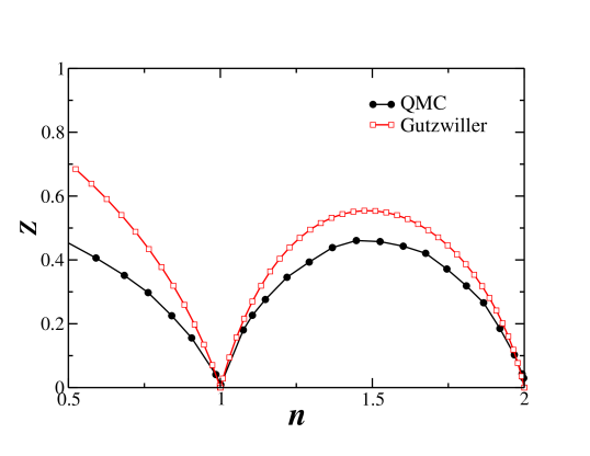
Figure 22: The quasiparticle residue $Z$ from the Gutzwiller method (open squares) is compared to the QMC $Z$ (full circles) extracted from imaginary axis data. Calculations were performed for the two–band Hubbard model on Bethe lattice with $U=4D$ for QMC and $U=5.8D$ for the Gutzwiller. The later value was chosen to keep ratio $U/U_{MIT}$ the same in both methods. MIT denotes metal-insulator transition.

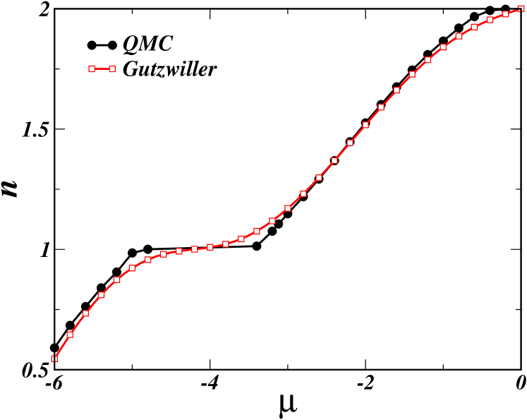
Figure 23: Doping versus chemical potential extracted from QMC (circles) and from the Gutzwiller method (squares) for two–band Hubbard model on Bethe lattice with $U=4D$.

In Fig. 22, we show a comparison between QMC and Gutzwiller quasiparticle renormalization amplitude $Z$ for the two–band Hubbard model on Bethe lattice. We notice that the Gutzwiller method captures all the basic low–frequency features of the model and compares very favorably with the QMC results. Remarkably, the chemical potential also shows a very good agreement between QMC and the Gutzwiller method as can be seen in Fig. 23.

The slave boson technique constructed in Ref. Kotliar and Ruckenstein (1986) is closely related and inspired by the famous Gutzwiller approximation, which appears as the saddle point of the functional integral in terms of the auxiliary boson fields describing the local collective excitations of the system. However there is a conceptual difference: rather than attempting to estimate the total energy, the slave boson approach constructs an approximation for the Green’s function at low energy Eq. (252). Fluctuations around the saddle point, then allow to recover the Hubbard bands as demonstrated in references Castellani et al. (1992); Read and Newns (1983); Read (1985); Lavagna (1990). The Gutzwiller approximation to the Gutzwiller wave function becomes exact in infinite dimensions Metzner and Vollhardt (1988) and has been recently evaluated in the general multiorbital case Bünemann and Weber (1997); Bünemann et al. (1998). In the limit of density-density interactions, the form of the renormalization function $z$ is identical to the one obtained from the slave boson method. The Gutzwiller approach is an approach that gives the total energy, and also the Green’s function if one makes the slave boson identification connecting the Gutzwiller renormalization factor to the Green’s function. It has been applied to Iron and Nickel by Bünneman and Weber Bünemann et al. (2003); Ohm et al. (2002). Additionally, the slave boson method gives the exact solution for the Mott transition in a system with large orbital degeneracy Florens et al. (2002).

III.6 Interpolative schemes

This section covers a different type of approximation to the functional $\Sigma(E_{imp},\Delta)$. These are not controlled approximations, in the sense that they are not based on a small parameter, but instead are attempts to provide approximations which are valid simultaneously for weak and strong coupling, high and low frequency, by combining different techniques as well as additional exact information. By combining various bits of information and various approaches one can obtain the self–energy which is more accurate over a broader range of parameters. Their accuracy has to be tested against more expensive and exact methods of solution.

III.6.1 Rational interpolation for the self–energy

The iterative perturbation theory (IPT) method was very successful in unraveling the physics of the Mott transition in the one–band Hubbard model. Its success is due to the fact that it captures not only the band limit but also the atomic limit of the problem at half filling. As we will show in section III.6.2, the extensions of the IPT method are possible, but less reliable in the multiorbital case. There have been some attempts to “define” interpolative methods that are robust enough and give reasonable results in the whole space of parameters of an multiorbital impurity model.

In this section, we will review the ideas from Savrasov et al. (2004) where a simple rational form for the self–energy was proposed and unknown coefficient from that rational expression were determined using the slave boson mean–field (SBMF) method. This scheme tries to improve upon SBMF, which gives the low–frequency information of the problem, by adding Hubbard bands to the solution. For simplicity, only $SU(N)$ symmetry will be considered.

It is clear that Hubbard bands are damped atomic excitations and to the lowest order approximation, appear at the position of the poles of the atomic Green’s function. Therefore, a good starting point to formulate the functional form for the self–energy might be the atomic self–energy

$$\Sigma^{(at)}(i\omega)=i\omega-\varepsilon_{f}-\left[G^{(at)}(i\omega)\right]^{-1},$$ (253)

where

$$G_{at}(i\omega)=\sum_{n=0}^{N-1}\frac{C_{n}^{N-1}(\tilde{P}_{n}+\tilde{P}_{n+1})}{i\omega+\mu-E_{n+1}+E_{n}},$$ (254)

and $E_{n}=\varepsilon_{f}n+\frac{1}{2}Un(n-1)$, $\tilde{P}_{n}$ is the probability to find an atom in a configuration with $n$ electrons, and $C_{n}^{N-1}=\frac{(N-1)!}{n!(N-n-1)!}$ arises due to the equivalence of all states with $n$ electrons in $SU(N)$.

The atomic self–energy can also be brought into the form

$$\Sigma^{(at)}(i\omega)=i\omega-\varepsilon_{f}-\frac{\prod\limits_{i=1}^{N}(i\omega-Z_{i})}{\prod\limits_{i=1}^{N-1}(i\omega-P_{i})},$$ (255)

where $Z_{i}$ are zeros and $P_{i}$ are the $N-1$ poles, which can be calculated from equations (253) and (254). Using the same functional form (255) for the self–energy at finite $\Delta$ and calculating probabilities $X_{n}$ self–consistently results in the famous Hubbard I approximation.

To add the quasiparticle peak in the metallic state of the system, one needs to add one zero and one pole to Eq. (255). To see this, let us consider the SU(N) case for the Hubbard model where the local Green’s function can be written by the following Hilbert transform $G_{loc}(\omega)=H(\omega-\varepsilon_{f}-\Sigma(\omega))$. If self–energy lifetime effects are ignored, the local spectral function becomes $A_{loc}=D(\omega-\varepsilon_{f}-\Sigma(\omega))$ where $D$ is the non–interacting density of states. The peaks in spectral function thus appear at zeros $Z_{i}$ of Eq. (255) and to add a quasiparticle peak, one needs to add one zero $Z_{i}$. To make the self–energy finite in infinity, one also needs to add one pole $P_{i}$ to Eq. (255). This pole can control the width of the quasiparticle peak. By adding one zero and one pole to the expression (255), the infinite frequency value of the self–energy is altered and needs to be fixed to its Hartree–Fock value. The pole which is closest to zero is the obvious candidate to be changed in order to preserve the right infinite value of the self–energy. The functional form for the self–energy in the metallic state of the system can take the following form

$$\Sigma(i\omega)=i\omega-\varepsilon_{f}-\frac{(i\omega-X_{1})\prod\limits_{i=1}^{N}(i\omega-Z_{i})}{(i\omega-X_{2})(i\omega-X_{3})\prod\limits_{i=1}^{N-2}(i\omega-P_{i})}.$$ (256)

To compute the $2N+1$ unknown coefficients in Eq. (256), the following algorithm was used in Savrasov et al. (2004)

• All $N$ zeros $Z_{i}$ are computed from the atomic form of the self–energy Eq. (253) and probabilities $X_{n}$ are calculated by the SBMF method.

• Poles of the atomic self–energy are also computed from Eq. (253) with $X_{n}$ obtained by SBMF. All but one are used in constructing self–energy in Eq.(256). The one closest to Fermi level needs to be changed.

• The self–energy at the Fermi level $\Sigma(0)$ is given by the Friedel sum–rule

  $$\langle n\rangle = \frac{1}{2}+\frac{1}{\pi}\mathrm{arctg}\left(\frac{\epsilon_{f}+\Re\Sigma(i0^{+})+\Re\Delta(i0^{+})}{\hbox{Im}\Delta(i0^{+})}\right)$$ (257)

  $$+ \int\limits_{-i\infty}^{+i\infty}\frac{dz}{2\pi i}G_{f}(z)\frac{\partial\Delta(z)}{\partial z}e^{z0^{+}}.$$

  This relation is used to determine one of three unknown coefficients $X_{i}$.

• The slope of the self–energy at zero frequency is used to determine one more unknown coefficient. The quasiparticle weight $z$ is calculated by the SBMF method and the following relationship is used

  $$\frac{{\partial\Re\Sigma}}{{\partial}\omega}\mid_{\omega=0}=1-z^{-1}.$$ (258)

• Finally, the infinite frequency Hartree–Fock value of $\Sigma$ is used to determine the last coefficient in Eq. (256)

The $2N+1$ coefficients can be computed very efficiently by solving a set of linear equations. The method is thus very robust and gives a unique solution in the whole space of parameters. It’s precision can be improved by adding lifetime effects, replacing $\omega$ by second order self–energy in the way it is done in section III.6.2.

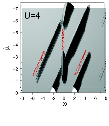
Figure 24: The density of states calculated by the rational interpolative method plotted as a function of the chemical potential $\tilde{\mu}=-\epsilon_{f}-(N-1)U/2$ and frequency for the two–band Hubbard model with $SU(4)$ symmetry and at $U=4D$.

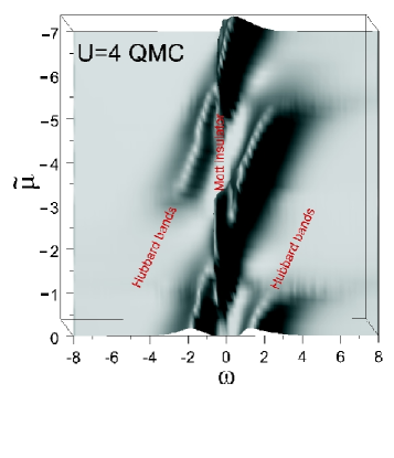
Figure 25: The density of states calculated by the QMC method plotted as a function of the chemical potential $\tilde{\mu}=-\epsilon_{f}-(N-1)U/2$ and frequency for the two–band Hubbard model within $SU(4)$ and at $U=4D$.

A typical accuracy of the method is illustrated in Fig. 24 by plotting the density of states as a function of the effective chemical potential $\tilde{\mu}=-\epsilon_{f}-(N-1)U/2$ and frequency in the regime of strong correlations. The corresponding QMC results are shown in 25 for comparison. Several weak satellites can also be seen on this figure (many atomic excitations are possible) which decay fast at high frequency.

The semicircular quasiparticle band, which is strongly renormalized by interactions, is seen at the central part of the figure. For the doping levels $\tilde{\mu}$ between 0 and -1 and between -3 and -5, the weight of the quasiparticle band collapses while lower and upper Hubbard bands acquire all the spectral weight. In the remaining region of parameters, both strongly renormalized quasiparticle bands and Hubbard satellites remain. When the bands are fully filled or emptied, the quasiparticle band restores its original bandwidth and the Hubbard bands disappear. From Fig. 24 and 25 it is clear that the rational interpolation for the self–energy in combination with the SBMF offers a satisfactory qualitative and quantitative solution of the multiorbital AIM which is useful for many applications of the LDA+DMFT to realistic systems.

III.6.2 Iterative perturbation theory

In this subsection we describe a different iterative perturbation theory which uses the second order self–energy Eq. (167) as a main building block and also achieves correct limits in the large frequency, zero frequency, band and atomic coupling limit. The idea originates from the fact that the second order perturbation theory works surprisingly well in the case of half–filled one–band Hubbard model and captures all the essential physics of the model. The success of this approach can be understood by noticing that $\Sigma^{(2)}$ from Eq. (167) gives the correct atomic limit although it is expected to work only in the weak coupling limit. The naive extension away from half–filling or for the multiband model treatment, however, fails because the latter property holds only in the special case of the half–filled one–band model. To circumvent this difficulty, a scheme can be formulated such that the atomic limit is also captured by the construction. In the following discussion, only $SU(N)$ symmetry will be considered.

To combine various bits of information in a consistent scheme, an analytic expression for the self–energy in the form of continuous fraction expansion

$${\Sigma}_{\alpha}(i\omega)={\Sigma}_{\alpha}(\infty)+\frac{A_{\alpha}}{i\omega-B_{\alpha}-\frac{C_{\alpha}}{i\omega-D_{\alpha}-\cdots}},$$ (259)

was set up in Ref. Oudovenko et al. (2004a). All the necessary coefficients, ${\Sigma_{\alpha}}(\infty),A_{\alpha},B_{\alpha},C_{\alpha}$, $D_{\alpha}$ …, can be determined by imposing the correct limiting behavior at high and low frequencies. The basic assumption of this method is that only a few poles in the continuous fraction expansion (259) are necessary to reproduce the overall frequency dependence of the self–energy.

Let us continue by examining the atomic limit of the second order self–energy Eq. (167) when evaluated in terms of the bare propagator $G^{0}_{\beta}(i\omega)=1/(i\omega+\widetilde{\mu}_{0}-\Delta_{\beta})$

$$\Sigma^{(2)}_{\alpha\;\Delta\rightarrow 0}={\gamma_{\alpha}\over i\omega+\widetilde{\mu}_{0}},$$ (260)

where $\gamma_{\alpha}=\sum_{\beta}(U_{\alpha\beta})^{2}n^{0}_{\beta}(1-n^{0}_{\beta})$ and $n^{0}_{\beta}$ is a fictitious particle number

$$n^{0}_{\beta}={1\over\pi}\int f(\omega){\rm Im}G^{0}_{\beta}(\omega-i0^{+})d\omega,$$ (261)

associated with bare propagator. The choice of $\tilde{\mu}_{0}$ will be discussed later.

The continuous fraction expansion in Eq. (259) can be made exact in the restricted atomic limit, i.e., when the three significant poles are considered in the Green’s function, and coefficients are calculated from the moments of the self–energy. By replacing $i\omega$ with $\gamma_{\alpha}/\Sigma^{(2)}_{\alpha}-\widetilde{\mu}_{0}$ in expansion Eq. (259), it is clear from Eq. (260) that the resulting self–energy functional has the correct atomic limit and reads

$$\Sigma_{\alpha}(i\omega)=\Sigma_{\alpha}(\infty)+{{A_{\alpha}\over\gamma_{\alpha}}\Sigma^{(2)}_{\alpha}\over 1-{\widetilde{\mu}_{0}+B_{\alpha}\over\gamma_{\alpha}}\Sigma^{(2)}_{\alpha}-{{(C_{\alpha}/\gamma_{a}^{2})}\left(\Sigma^{(2)}_{\alpha}\right)^{2}\over 1-(\widetilde{\mu}_{0}+D_{\alpha})\Sigma^{(2)}_{\alpha}/\gamma_{\alpha}-\cdots}}.$$ (262)

Coefficients $A$, $B$, $C$ and $D$ can be determined from the moment expansion

$$A_{\alpha}=\Sigma_{\alpha}^{(1)},$$ (263)

$$B_{\alpha}=\frac{\Sigma_{\alpha}^{(2)}}{\Sigma_{\alpha}^{(1)}},$$ (264)

$$C_{\alpha}=\frac{\Sigma_{\alpha}^{(3)}\Sigma_{\alpha}^{(1)}-(\Sigma_{\alpha}^{(2)})^{2}}{(\Sigma_{\alpha}^{(1)})^{2}},$$ (265)

where the self–energy moments can be expressed in terms of the density–density correlation functions (see Ref. Oudovenko et al. (2004a)).

Finally, the parameter $\widetilde{\mu}_{0}$ can be determined by imposing the Friedel sum rule, which is a relation between the total density and the real part of the self–energy at zero frequency, thereby achieving the correct zero frequency limit. Since the Friedel sum rule is valid only at zero temperature, the parameter $\widetilde{\mu}_{0}$ is determined at $T=0$, and after having it fixed, equation (262) is used at arbitrary temperatures.

An alternative scheme for determining the temperature–dependent $\widetilde{\mu}_{0}$ was proposed by Potthoff et al. Potthoff et al. (1997), and consists of the requirement that the fictitious occupancy computed from $G^{0}$ equals the true occupancy computed from $G$ Martín-Rodero et al. (1982). A careful comparison of these approaches was carried out by Potthoff et al. Potthoff et al. (1997); Meyer et al. (1999).

Note that one could continue the expansion in continuous fraction to the order in which the expansion gives not only restricted but the true atomic limit. However, in practice this is seldom necessary because only few poles close to the Fermi energy have a large weight.

It is essential that the self–energy Eq. (262) remains exact to $U^{2}$, which can be easily verified by noting that in the $U\rightarrow 0$ the fictitious occupancy $n^{0}$ approaches $n$ therefore $A_{\alpha}=\gamma_{\alpha}(1+O(U))$, $B\rightarrow-\widetilde{\mu}_{0}$ and $C\rightarrow 0$. At the same time, the self–energy Eq. (262) has correct first moment because expanding $\Sigma^{(2)}$ in the high–frequency limit yields $\Sigma_{\alpha}^{(2)}=\gamma_{\alpha}/(i\omega)+...$ and $A_{\alpha}$ is exact first moment.

Note that in the case of one–band model, the atomic limit requires only one pole in self–energy therefore the coefficient $C$ in Eq. (262) can be set to zero and one has

$$\Sigma_{\alpha}(i\omega)=\Sigma_{\alpha}(\infty)+{{A_{\alpha}\over\gamma_{\alpha}}\Sigma^{(2)}_{\alpha}\over 1-{\widetilde{\mu}_{0}+B_{\alpha}\over\gamma_{\alpha}}\Sigma^{(2)}_{\alpha}}.$$ (266)

Furthermore, double and triple occupancies do not enter the expression for the moments in the case of one–band model. If one chooses the functional form for the moments in the atomic limit, the interpolative self–energy (262) has still the same limiting behavior as discussed above. In this case, no additional external information is necessary and the system of equations (266), (263), (264) and (167) is closed.

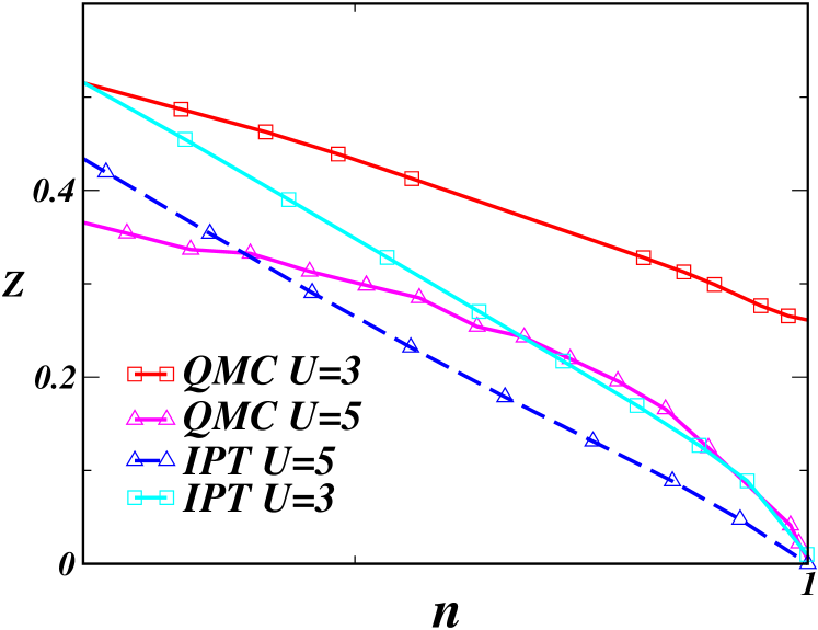
Figure 26: Comparison between QMC and the simplified IPT Eq. (266) renormalization amplitude $Z$ for the three–band Hubbard model on Bethe lattice at $U=3D$ and $5D$. QMC $Z$ was extracted at temperature $T=1/16$ and IPT at zero temperature.

For the multiband model, an approximate method is needed to calculate moments which in turn ensure a limiting form consistent with the simplified atomic limit. Many approaches discussed in previous sections can be used for that purpose, for example the Gutzwiller method or SUNCA. In Ref. Kajueter (1996b) the coherent potential approximation (CPA) was used to obtain moments in the functional form consistent with the atomic limit, i.e., neglecting last term in Eq. (264). Another possibility, also tested by Ref. Kajueter (1996b), is to use the ansatz Eq. (266) in the case of multiband model. In Fig. 26 the quasiparticle renormalization amplitude $Z$ versus particle number $n$ is displayed for $n$ less than one where this scheme compares favorably with the QMC method. CPA was used to obtain moments.

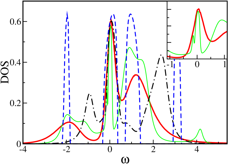
Figure 27: Density of states for the two–band Hubbard model on Bethe lattice at $U=2.5D$ and $n_{d}=1.1$. The tick full line marks QMC curve at temperature $T=1/16D$ while the rest of the curves correspond to various IPT schemes at $T=0$. The thin full line shows the IPT from Eq. (262) with all four coefficients determined by high–frequency moments in the functional form of atomic limit. The inset zooms the region around the chemical potential where the above mentioned IPT scheme develops a spurious double peak structure. The dot–dashed line corresponds to simplified IPT Eq. (266) with both two coefficients determined by moments. Finally, the dashed curve stands for the IPT schemes described in section III.6.1.

When the particle number slightly exceeds unity, the simplified IPT scheme Eq. (266) does not provide an accurate description of the multiorbital AIM. As shown in Fig. 27, the Hubbard bands are completely misplaced. Nevertheless, the quasiparticle peak is in good agreement with QMC result. By taking into account more terms in the continuous fraction expansion Eq. (262), the high–frequency part of spectra can be considerably improved since the resulting approximation obeys more high–frequency moments. Unfortunately, the quasiparticle peak develops a spurious double peak structure which severely limits the applicability of the method, as shown in the inset of Fig. 27. Systematically improving only the high–frequency part of the spectra, by incorporating more moments into the approximation, can thus spoil the low–frequency part. This type of unphysical feature can be avoided using the scheme from subsection III.6.1 where the derivative as well as the value of the spectra at zero frequency was imposed by the information obtained by a more accurate technique at low frequency, such as the Gutzwiller method.

The most general extension of IPT, and its simplified form Eq. (266) was set up in Ref. Kajueter (1996b) and in Ref. Martín-Rodero et al. (1982). The authors in Ref. Ferrer et al. (1987); Yeyati et al. (1999) tested it in the context of quantum dots, where it performs satisfactorily. However, Ref. Kajueter (1996b) tested it in the DMFT context, and the difficulties with the spurious double peak structure shown in Fig. 27 were found close to integer filling in the case of occupancies larger than one. When the occupancies are less than one, the simpler formula Eq. (266) is accurate and free from pathologies. It was used to compute the physical properties of ${\rm La}_{1-x}{\rm Sr}_{x}{\rm TiO}_{3}$ in Refs. Anisimov et al. (1997a); Kajueter et al. (1997). Various materials with strongly correlated $d$–bands were studied by the group of Craco, Laad and Müller-Hartmann using the IPT method for arbitrary filling of the correlated bands. The properties of ${\rm CrO_{2}}$ Laad et al. (2001); Craco et al. (2003b), ${\rm LiV_{2}O_{4}}$ Laad et al. (2003a), ${\rm V_{2}O_{3}}$ Laad et al. (2003b) and ${\rm Ga_{1-x}Mn_{x}As}$ Craco et al. (2003a) were explained by the IPT method.

IV Application to materials

In this section we illustrate the realistic dynamical mean–field methodology with examples taken from various materials. We chose situations where correlations effects are primarily responsible for the behavior of a given physical system. The examples include: (i) phase transitions between a metal and insulator where, in the absence of any long–range magnetic order, opening an energy gap in spectrum cannot be understood within simple–band theory arguments; (ii) large, isostructural volume collapse transitions where a localization–delocalization driven change in lattice parameters of the system is necessary to understand the transition; (iii) the behavior of systems with local moments which are not straightforward to study within band theory methods. We conclude this section with a brief, non–comprehensive summary of a few other illustrations of the power of the dynamical mean–field method that, for lack of space, cannot be covered in this review.

IV.1 Metal–insulator transitions

IV.1.1 Pressure driven metal–insulator transitions

The pressure driven metal–insulator transition (MIT) is one of the simplest and at the same time most basic problems in the electronic structure of correlated electrons. It is realized in many materials such as V₂O₃, where the metal–insulator transition is induced as function of chemical pressure via Cr doping, quasi–two–dimensional organic materials of the $\kappa$ family such as (BEDT–TSF)₂X (X is an anion) Ito et al. (1996); Lefebvre et al. (2000), and Nickel Selenide Sulfide mixtures (for a review see Imada et al. (1998) as well as articles of Rosenbaum and Yao in Edwards and Rao (1990)). The phase diagram of these materials is described in Fig. 28. It is remarkable that the high–temperature part of the phase diagram of these materials, featuring a first order line of metal–insulator transitions ending in a critical point, is qualitatively similar in spite of the significant differences in the crystal and electronic structure of these materials  Kotliar (1999b); Chitra and Kotliar (1999); Kotliar (2001). This is illustrated in Fig. 29 where the schematic phase diagram of the integer filled Hubbard model is included.

V₂O₃ has a Corundum structure in which the V ions are arranged in pairs along the $c$ hexagonal axis, and form a honeycomb lattice in the basal $ab$ plane. Each V ion has a $3d^{2}$ configuration. The $d$–electrons occupy two of the $t_{2g}$ orbitals which split into a non–degenerate $a_{1g}$ and a doubly degenerate $e_{g}^{\pi}$ orbital. The $e_{g}^{\sigma}$ states lie higher in energy Castellani et al. (1978a, b). NiSeS mixtures are charge transfer insulators, in the Zaanen–Sawatzky–Allen classification Zaanen et al. (1985), with a pyrite structure. In this compound the orbital degeneracy is lifted, the configuration of the $d$–electron in Ni is spin one, $d^{8}$, and the effective frustration arises from the ring exchange in this lattice structure. The $\kappa$ -(BEDT–TSF)₂X (X is an anion) Ito et al. (1996); Lefebvre et al. (2000) are formed by stacks of dimers and the system is described at low energies by a one–band Hubbard model with a very anisotropic next nearest neighbor hopping  McKenzie (1998); Kino and Fukuyama (1996).

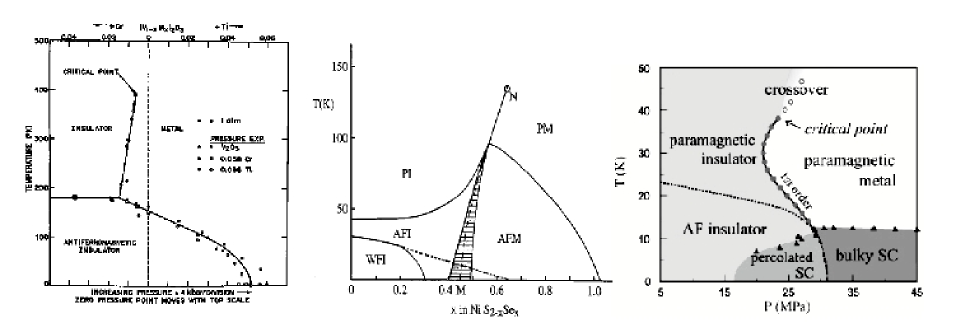
Figure 28: The phase diagrams of V₂O₃, NiS_2-xSe_x and organic materials of the $\kappa$ family (from McWhan et al. (1971) (left), Edwards and Rao (1990) (middle), and Kagawa et al. (2004) (right)).

The universality of the Mott phenomena at high temperatures allowed its description using fairly simple Hamiltonians. One of the great successes of DMFT applied to simple model Hamiltonians was the realization that simple electronic models are capable of producing such phase diagram and many of the observed physical properties of the materials in question. The qualitative features related to the Mott transition at finite temperature carry over to more general models having other orbital and band degeneracy as well as coupling to the lattice. The dependence of this phase diagram on orbital degeneracy has been investigated recently Florens et al. (2002); Ono et al. (2003); Kajueter and Kotliar (1997); Ono et al. (2001).

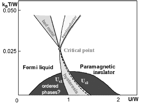
Figure 29: Schematic phase diagram of a material undergoing a Mott metal–insulator transition.

The determination of the extension of the qualitative phase diagram away from half filling includes regions of phase separation near half filling Kotliar et al. (2002). Determination of the low–temperature phases, which are completely different in the materials in Fig. 28, requires a more careful and detailed modeling of the material, and the study of the dependence of the magnetic properties on the properties of the lattice is only in the beginning stages Chitra and Kotliar (1999); Zitzler et al. (2004).

Dynamical mean–field theory Georges et al. (1996), provided a fairly detailed picture of the evolution of the electronic structure with temperature and interaction strength or pressure. Surprising predictions emerged from these studies: a) the observation that for a correlated metal, in the presence of magnetic frustration, the electronic structure (i.e. the spectral function) contains both quasiparticle features, and Hubbard bands Georges and Kotliar (1992). b) The idea that the Mott transition is driven by the transfer of spectral weight from the coherent to the incoherent features Zhang et al. (1993). This scenario, brought together the Brinkman–Rice–Gutzwiller ideas and the Hubbard ideas about the Mott transition in a unified framework. c) The existence of broad regions of parameters where the incoherent part of the spectra dominates the transport. The impurity model subject to the DMFT self–consistency condition is a minimal model to approach the understanding of the incoherent or bad metal, the Fermi liquid state, the Mott insulating state, and a “semiconducting” or “bad insulator” state where thermally induced states populate the Mott Hubbard gap. d) An understanding of the critical behavior near the Mott transition as an Ising transition Kotliar et al. (2000). This critical behavior had been surmised long ago by Castellani et al.  Castellani et al. (1979).

In the last few years experimental developments have confirmed many of the qualitative predictions of the DMFT approach. For recent reviews see  Kotliar and Vollhardt (2004); Georges (2004a, b).

a) Photoemission spectroscopy has provided firm evidence for a three peak structure of the spectral function in the strongly correlated metallic regime of various materials and its evolution near the Mott transition. This was first observed in the pioneering experiments of A. Fujimori et al.  Fujimori et al. (1992b). The observation of a quasiparticle peak near the Mott transition took some additional work. In Ref. Matsuura et al. (1998), angle resolved photoemission spectra in NiSeS reveal the presence of a quasiparticle band and a Hubbard band (see Figs.  30,31).

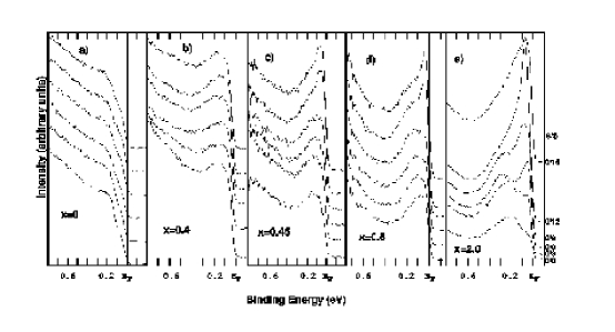
Figure 30: Near–Fermi–level ARPES spectra in NiSeS taken nearly along the (001) direction for (a) $x=0$ (insulating), (b) $x=0.4$ (insulating), (c) $x=0.45$ (metallic), (d) $x=0.5$ (metallic), and (e) $x=2.0$ (metallic) (from Ref. Matsuura et al. (1998)).

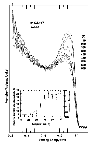
Figure 31: Temperature–dependence obtained in NiSeS of the near- $\varepsilon_{F}$ peak for $x=0.45$ at 22.4 eV incident photon energy. Inset: Distance of the 50% point of the leading edge from $\varepsilon_{F}$ (solid circles); reactivity (open circles, right–hand scale); area under the near-$\varepsilon_{F}$ peak (solid diamonds, scaled in arbitrary units). Analyzer angle: $0/9$ (from Ref. Matsuura et al. (1998)).

These results, together with a DMFT calculation by Watanabe and Doniach, in the framework of a two–band model are shown in Fig. 32.

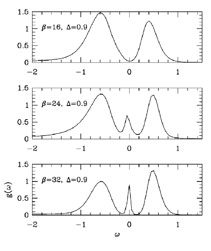
Figure 32: Single–particle Green’s functions at half–filling for a fixed charge–transfer gap and varying temperature. Horizontal axis is scaled in units of $2t$. Vertical axis has arbitrary units (from Ref. Matsuura et al. (1998)).

Cubic SrVO₃ and orthorhombic CaVO₃ perovskites are strongly correlated metals. LDA+DMFT calculations  Sekiyama et al. (2004) find their spectral functions to be very similar in agreement with recent bulk–sensitive photoemission experiments Sekiyama et al. (2002, 2004). The comparison of the high–energy LDA+DMFT photoemission results against the experiments is presented in Fig. 33. LDA qualitatively fails as it cannot produce the Hubbard band while LDA+DMFT successfully captures this and compares well with experiment.

Figure 33: A comparison of LDA (panel $a$), LDA+DMFT (panel $d$), and the photoemission data for $SrVO_{3}$ and $CaVO_{3}$ (after Sekiyama et al. (2004)).

Using high–energy photoemission spectroscopy, Mo et al.  Mo et al. (2003) studied the V₂O₃ system. The spectral function, which exhibits a quasiparticle peak and a Hubbard band, is displayed in Fig. 34 together with an LDA+DMFT calculation. The calculation was performed using the LDA density of states of the Vanadium $t_{2g}$ electrons and a Hubbard $U$ of 5 eV.

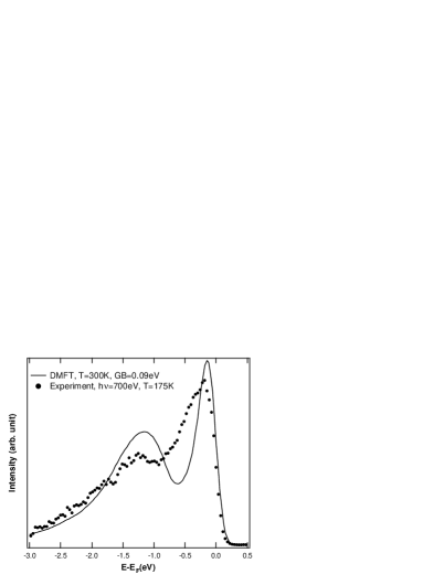
Figure 34: Comparison of $h\nu=700$ eV PES spectrum with LDA+DMFT(QMC) spectrum for $T=300$ K and $U=5.0$ eV in $V_{2}O_{3}$. (after Mo et al. (2003))

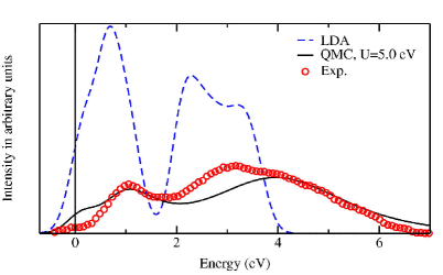
Figure 35: Comparison of the LDA and LDA+DMFT(QMC) spectra at $T=0.1$ eV (Gaussian broadened with 0.2 eV) with the x–ray absorption data of Müller et al. (1997) in $V_{2}O_{3}$. The LDA and QMC curves are normalized differently since the $\epsilon_{g}^{\sigma}$ states, which are shifted towards higher energies if the Coulomb interaction is included, are neglected in our calculation (from Ref. Held et al. (2001a)).

b) Optical spectroscopy has confirmed the idea of temperature driven transfer of spectral weight in the vicinity of the Mott transition. The first indications had been obtained in the V₂O₃ system Rozenberg et al. (1995) where it was found that as temperature is lowered, optical spectral weight is transferred from high energies to low energies. Similar observations were carried out in NiSeS  Miyasaka and Takagi (2004), and in the kappa organics Eldridge et al. (1991), confirming the high–temperature universal behavior of materials near a Mott transition.

c) The Ising critical behavior predicted by DMFT is now observed in Cr doped V₂O₃  Limelette et al. (2003a). The large critical region and the experimental observation of the spinodal lines (Figs. 36 and 37), was ascribed to the importance of electron–phonon coupling Kotliar (2003). The situation in organic materials at this point is not clear Kagawa et al. (2003); Kanoda (2004).

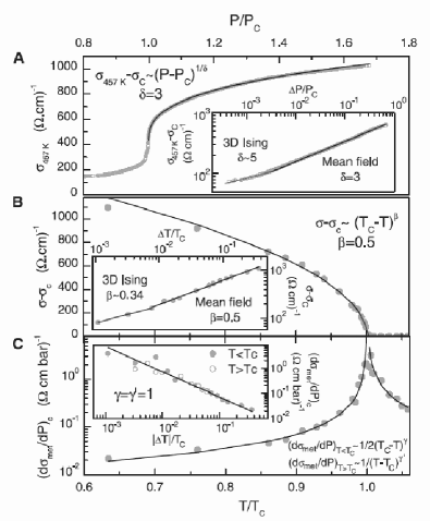
Figure 36: Temperature dependence of the conductivity (a), the order parameter (b) and derivative of the conductivity (analogous to a susceptibility) (c) in Cr doped V₂O₃ (from Ref. Limelette et al. (2003a)).

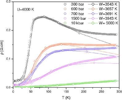
Figure 37: Temperature–dependence of the resistivity in Cr doped V₂O₃ at different pressures. The data (circles) are compared to a DMFT–NRG calculation (diamonds), with a pressure dependence of the bandwidth as indicated. The measured residual resistivity $\rho_{0}$ has been added to the theoretical curves (from Ref. Limelette et al. (2003b)).

e) Transport studies in V₂O₃ Kuwamoto et al. (1980) and in NiSeS Imada et al. (1998) have mapped out the various crossover regimes of the DMFT phase diagram (see Fig.  29), featuring a bad metal, a bad insulator, a Fermi liquid and a Mott insulator. More recent studies in the two–dimensional kappa organics Limelette et al. (2003b) are consistent with the DMFT picture, and can be fit quantitatively within single–site DMFT (see Fig. 38).

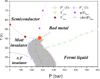
Figure 38: Pressure–Temperature phase diagram of the $\kappa$-Cl salt (from Ref. Limelette et al. (2003b)).

The dynamical mean field studies have settled a long standing question. Is the Mott transition in V₂O₃, NiSSe and kappa organics driven by an electronic structure mechanism or by the lattice (i.e. the position of the ions ) degrees of freedom.

This question can only be answered theoretically since lattice deformations are almost always generically induced by changes in the electronic structure (see below) and vice–versa. In a theoretical study one can freeze the lattice while studying a purely electronic model, and it is now accepted that the simple Hubbard model can account for the topology of the high temperature phase diagram Georges et al. (1996). Hence, lattice deformations are not needed to account for this effect even though they necessarily occur in nature. A cluster study of the frustrated, two-dimensional Hubbard model using CDMFT (ie. 2x2 plaquette)  Parcollet et al. (2004) demonstrated that the single site DMFT statement of the existence of a finite temperature Mott transition survives cluster corrections, even though qualitative modifications of the single site DMFT results appear at lower temperatures or very close to the transition. Finally new numerical approaches to treat systems directly on the lattice have further corroborated the qualitative validity of the single site DMFT results Onoda and Imada (2003).

Figure 39: Schematic volume dependence of free energy for a model within DMFT.

The fact that the coupling of the lattice is important near the electronically driven Mott transition was first pointed out in the dynamical mean field context in ref Majumdar and Krishnamurthy (1994). The electronic degrees of freedom are divided into those described by the low energy model Hamiltonian (see section I.2.5) and the rest, and the total free energy of the system is given by the sum of these two contributions $F_{other}$ and $F_{model}$. These free energies depend on the volume of the material. Formally the energy of the model Hamiltonian is a function of the model Hamiltonian parameters such as the bandwidth $t$ and Coulomb interaction $U$, but these parameters themselves depend on volume.

We have seen that in the absence of elastic interactions the Hubbard model has two solutions, a metallic and an insulating one, in a range of values of $U/t$. Hence $F_{model}(t(V))$ can have two branches which cross as depicted in Fig. 39. The free energy curve obtained by picking at each volume the lowest of the free energies has a cusp singularity (an infinitely negative second derivative at the critical volume)indicating the formation of a double well structure.

The addition of $F_{other}$, which by construction is smooth, cannot qualitatively modify this behavior. Furthermore, the double well structure, which must exist below the Mott transition temperature, also must persist slightly above the Mott transition point (given the infinite second derivative at the critical volume below the transition point of the model Hamiltonian). The position where the double well develops signals the position of the true (i.e. renormalized by the lattice ) metal to insulator transition. The exact free energy is a concave function of the volume and this concavity which is missed in mean field theory, is restored through a Maxwell construction.

This qualitative discussion sketches how the spectral density functional theory formalism is used to predict the volume of materials starting from first principles. The self-consistent application of LDA+DMFT determines the energy of model Hamiltonian and the one electron Hamiltonian of both the low energy and the high energy degrees of freedom in a self-consistent fashion. Results for Ce and Pu are shown in Figs. 46 and  47, respectively. In materials where the model exhibits a transition, the LDA+DMFT studies produce a double well as will be discussed for Ce and Pu in sections IV.2.1 and IV.2.2, respectively.

It has been recently emphasized  Amadon et al. (2005) that in Cerium the double well is of purely entropic nature, while the calculations for Pu only include the energy, but the qualitative argument for the existence of a double well applies to the free energy of both materials. An analysis of the influence of the coupling to the lattice on the compressibility and the electron-phonon coupling has been carried out in  Hassan et al. (2004).

IV.1.2 Doping driven metal–insulator transition

Doping driven metal–insulator transitions in the three–dimensional perovskites La_1-xSr_xTiO_3-δ has been extensively explored in the past decade Tokura et al. (1993); IV et al. (1992); Maeno et al. (1990); Crandles et al. (1992); Onoda and Yasumoto (1997b, a); Onoda and Kohno (1998); Hays et al. (1999). The electronic properties of the La_1-xSr_xTiO₃ series is governed by the $t_{2g}$ subset of the $3d$ orbitals. When $x=0$, there is one electron per Ti, and the system is a Mott insulator. Doping with Strontium or Oxygen introduces holes in the Mott insulator.

In the cubic structure the $t_{2g}$ orbital is threefold degenerate, but this degeneracy is lifted by an orthorhombic distortion of the GdFeO₃ structure resulting in the space group $Pbnm$. For $x>0.3$ the material is found to transform to another distorted perovskite structure with space group $Ibmm$. For larger values of $x>0.8$ the orthorhombic distortion vanishes and the material assumes the cubic perovskite structure of SrTiO₃ with space group $Pm3m$. LaTiO₃ is a Mott insulator which orders antiferromagnetically at $T_{N}\approx 140$ K, with a Ti magnetic moment of 0.45 $\mu_{B}$ and small energy gap of approximately 0.2 eV.

The lifting of the degeneracy plays a very important role for understanding the insulating properties of this compound, and they have recently been discussed by a single–site DMFT study of this compound Pavarini et al. (2004). For moderate dopings La_1-xSr_xTiO₃ behaves as a canonical doped Mott insulator. The specific heat and the susceptibility are enhanced, the Hall coefficient is unrenormalized, and the photoemission spectral function has a resonance with a weight that decreases as one approaches half filling. Very near half filling, (for dopings less than 8 %) the physics is fairly complicated as there is an antiferromagnetic metallic phase  Kumagai et al. (1993); Okada et al. (1993); Onoda and Kohno (1998). While it is clear that the parent compound is an antiferromagnetic Mott insulator, the orbital character of the insulator is not well understood, as recent Raman scattering  Reedyk et al. (1997) and neutron scattering investigations reveal Furukawa et al. (1997, 1999).

Very near half–filling when the Fermi energy becomes very small and comparable with the exchange interactions and structural distortion energies, a treatment beyond single–site DMFT becomes important in order to treat spin degrees of freedom. Alternatively, for moderate and large dopings, the Kondo energy is the dominant energy and DMFT is expected to be accurate. This was substantiated by a series of papers reporting DMFT calculations of a single–band or multiband Hubbard model with a simplified density of states. Ref. Rozenberg et al. (1994) addressed the enhancement of the magnetic susceptibility and the specific heat as the half–filling is approached. The optical conductivity and the suppression of the charge degrees of freedom was described in Ref. Rozenberg et al., 1996, while the observation that the Hall coefficient is not renormalized was reported in Ref. Kotliar and Kajueter, 1996; Kajueter and Kotliar, 1997. The thermoelectric power was investigated by Pálsson and Kotliar Pálsson and Kotliar (1998) and the magnetotransport by Lange and Kotliar Lange and Kotliar (1999).

Given the simplicity of the models used and the various approximations made in the solution of the DMFT equations, one should regard the qualitative agreement with experiment as very satisfactory. The photoemission spectroscopy of this compound as well as of other transition metal compounds do not completely reflect the bulk data, and it has been argued that disorder together with modeling of the specific surface environment is required to improve the agreement with experiment  Sarma et al. (1996); Maiti et al. (2001). More realistic studies were carried out using LDA+DMFT. The results are weakly sensitive to the basis set used while more sensitive to the value of the parameter $U$ and impurity solver. This was discussed in section  III, and it becomes very critical for materials near the Mott transition since different impurity solvers give slightly different values of critical $U$, and hence very different physical spectra for a given value of $U$ Nekrasov et al. (2000); Held et al. (2001c). However, if we concentrate on trends, and take as a given that $U$ should be chosen as to place the material near or above the Mott transition, nice qualitative agreement with experiment is obtained.

Anisimov Anisimov et al. (1997a) considered a realistic Hamiltonian containing Oxygen, Titanium, and Lanthanum bands and solved the resulting DMFT equations using IPT. Nekrasov et al. Nekrasov et al. (2000) solved the DMFT equations using $t_{2g}$ density of states obtained from an LMTO calculation. In this procedure, the bare density of states is rescaled so that it integrates to one. They solved the DMFT equations using QMC, IPT and NCA.

Comparison of photoemission experiments with results obtained using the QMC impurity solver for different values of $U$ is presented in Fig. 40. One can find favorable agreement between experimental and LDA+DMFT results for $U=5$ eV. LDA+DMFT reproduce the quasiparticle and Hubbard bands while LDA captures only the spectra around the Fermi level.

Figure 40: Comparison of the experimental photoemission spectrum  Fujimori et al. (1992b, a); Yoshida et al. (2002), the LDA result, and the LDA+DMFT(QMC) calculation for LaTiO₃ with 6% hole doping and different Coulomb interaction $U=3.2$, 4.25, and 5 eV (from Ref. Nekrasov et al. (2000)).

The linear term of the specific heat coefficient was computed by fitting the $t_{2g}$ density of states to a tight–binding parameterization. To capture the asymmetry in tight–binding DOS the next nearest neighbor term, $t^{\prime}$, on Ti sublattice have to be taken into account. The dispersion which has been obtained from the fit is $\epsilon_{\bf k}=2t(\cos k_{x}+\cos k_{y})+2t^{\prime}\cos(k_{x}+k_{y})+2t_{\perp}\cos k_{z}$, where $t=-0.329664$, $t^{\prime}=-0.0816$, $t_{\perp}=-0.0205$ in eV units. Using the tight–binding DOS and the QMC impurity solver, the Green’s function and the specific heat were calculated. The specific heat is given in terms of the density of states $N(\mu)$ at the Fermi level by $\gamma=2.357\left[\frac{mJ}{molK^{2}}\right]\frac{N(\mu)[\mbox{states/(eV unit cell)}]}{Z}$ where $Z$ is the quasiparticle residue or the inverse of the electronic mass renormalization. In the LDA, the value of $Z$ is equal to one and the doping dependence can be computed within the rigid band model. The LDA+DMFT results are plotted against the experiment in Fig. 41. Despite some discrepancies, there is good semiquantitative agreement.

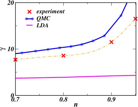
Figure 41: Filling dependence of the linear coefficient of specific heat, $\gamma$, of doped LaTiO₃ obtained from DMFT calculations using QMC as an impurity solver (solid line with stars) with $U=5$, temperature $\beta=16$ and LDA calculations (solid line). Experimental points are given by crosses and a dot–dashed line is used as a guide for eye. Tight–binding density of states was used in the self–consistency loop of the DMFT procedure. Energy unit is set to half bandwidth.

In general, the LDA data for $\gamma$ are much lower than the experimental values, indicating a strong mass renormalization. Also we note that as we get closer to the Mott–Hubbard transition the effective mass grows significantly. This is consistent with DMFT description of the Mott–Hubbard transition, which exhibits divergence of the effective mass at the transition.

Oudovenko et al. Oudovenko et al. (2004c) considered the optical properties of La_1-xSr_xTiO₃. The trends are in qualitative agreement with those of earlier model studies Kajueter and Kotliar (1997) but now the calculations incorporate the effects of realistic band structures. In Fig. 42 we plot the calculated optical conductivity for La_xSr_1-xTiO₃ at doping $x=0.1$ using the DMFT (solid line) and compare it with the experimental data (dashed line with open cycles symbols) measured by Fujishima et al. Fujishima et al. (1992) and with the LDA calculations (dot–dashed line). The low frequency behavior for a range of dopings is shown in Fig. 43.

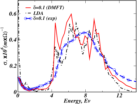
Figure 42: Calculated optical conductivity spectrum for La_xSr_1-xTiO₃, $x=0.10$, at large frequency interval using DMFT method as compared with the experimental data and results of the corresponding LDA calculations.

Figure 43: Low frequency behavior of the optical conductivity for La_1-xSr_xTiO₃ at $x=0.1,0.2,0.3$ calculated using the LDA+DMFT method. Experimental results Okimoto et al. (1995) are shown by symbols for the case $x=0.1$. In the inset the effective number of carriers is plotted as a function of doping. Squares show the results of the LDA+DMFT calculations. Circles denote the experimental data from Ref. Okimoto et al. (1995).

First we notice that the DMFT result agrees with the experiment up to the energy of 2 eV. Above 2 eV, both the LDA and DMFT optics are quite close and fit the experiment reasonably well.

Its worth emphasizing that corresponding calculations based on the local density approximation would completely fail to reproduce the doping behavior of the optical conductivity due to the lack of the insulating state of the parent compound LaTiO₃ within LDA. As a result, the LDA predicts a very large Drude peak even for zero doping, which remains nearly unchanged as a function of doping. In view of this data, DMFT captures the correct trend upon doping as well as the proper frequency behavior, which is a significant improvement over the LDA.

IV.1.3 Further developments

Understanding the simplest prototypes of the Mott transition within DMFT has opened the way to many investigations of modified and generalized models which are necessary to understand the rich physics of real materials. Materials with unfilled bands and very different bandwidth near the Fermi level (examples include ruthenates Ca_2-xSr_xRuO₄ Anisimov et al. (2002), CrO₂  Toropova et al. (2005), cobaltates  Ishida et al. (2005); Lechermann et al. (2005b), the classic Mott insulators VO₂ Goodenough (1971) and V₂O₃  Ezhov et al. (1999), in layered organic superconductors  Lefebvre et al. (2000), fullerenes  Takenobu et al. (2000), and many other compounds Imada et al. (1998)) raise the possibility of an orbitally selective Mott transition, where upon increase of the interaction $U$ one band can turn into an insulator while the other one remains metallic.

This was observed first in connection with the $\mathrm{Ca_{2-x}Sr_{x}RuO_{4}}$ system Nakatsuji and Maeno (2000); Nakatsuji et al. (2003) and also the $\mathrm{La_{n+1}Ni_{n}O_{3n+1}}$ system Sreedhar et al. (1994); Zhang et al. (1994); Kobayashi et al. (1996). The qualitative idea is that when two bands differ substantially in bandwidth, as the interaction strength is increased, there should be a sequence of Mott transitions, whereby first narrow band undergoes a localization transition with the broader band remaining itinerant while at large $U$ both bands are localized. The term orbital selective Mott transition (OSMT) was given for this situation Anisimov et al. (2002).

The Hubbard interaction is separated into $U$ among opposite spins, $U^{\prime}$ among different orbitals, and the flipping term, which is proportional to Hund’s coupling $J$.

This problem is receiving much attention recently. Most of the work was focused on the case of symmetric bands in the particle hole symmetric point. It has been shown that an OSMT is possible provided that the difference in bandwidth $t^{h}/t^{l}$ is small enough. The requirement on this ratio is made less extreme and therefore the OSMT more clearly visible as $J$ is increased, in particular if its spin rotationally invariant form is treated Anisimov et al. (2002); Koga et al. (2004, 2005); Ferrero et al. (2005); de’ Medici et al. (2005a); Arita and Held (2005); C. Knecht and N. Blümer and P. G. J. van Dongen (2005).

Interestingly, it was shown in references Biermann et al. (2005a) that in the regime where the heavy orbital is localized and the light orbital is itinerant, the heavy orbital forms a moment which scatters the light electron resulting in the type of non Fermi liquid behavior that was first found in the context of the Falikov Kimball model, and studied extensively in the context of manganites. This type of non Fermi liquid, containing light electrons scattered by local collective modes, is then realized in many situations in transition metal oxides.

The effects of interactions containing three electrons in the heavy bands and one electron in the light band have not been studied in detail. They can be eliminated at the expenses of generating a hybridization term, which at least in some cases, has been shown to be a relevant perturbation turning the insulating band into a metallic state via hybridization  de’ Medici et al. (2005b). Finally, we note that understanding this problem in the context of real materials will require the interplay of LDA band theory and DMFT many body calculations.

Bands are not necessarily symmetric and their center of gravity may be shifted relative to each other. The fundamental issue is how crystal field splittings and spin orbit splittings are renormalized by many body interactions. This is important not only for experiments which measure the orbital occupancies but also because the renormalization of the crystal field splitting is a relevant perturbation that can modify dramatically the nature of the OSMT. This is already seen in the atomic limit, where shifts in $\epsilon_{h}-\epsilon_{l}$ can have dramatic effect, even in static approaches. For example, in V₂O₃ Held et al. (2005); Held et al. (2001a); Keller et al. (2005) the “heavy” $a_{1g}$ orbital is quickly renormalized below the bottom of the LDA conduction band. Notice that if the heavy orbital is moved well above the light orbital, one can have an essentially weakly correlated situation, while if the heavy orbital moves well below the light orbital and if the number of electrons is such that the heavy orbital is not full, one encounters a situation where local collective modes scatter the light electrons.

A related issue is how interactions renormalize the Fermi surface beyond the LDA Fermi surface. While in many cases the LDA Fermi surface provides a good approximation to the true Fermi surface of many materials such as heavy fermions, there are materials where this is not the case. The issue was first raised in connection with De Haas van Alphen and photoemission experiments on CaVO₃ Inoue et al. (2002) and SrRuO₄ Kikugawa et al. (2004) (for a review see Mackenzie and Maeno (2003)). This problem was first approached theoretically by Liebsch and Lichtenstein using DMFT Liebsch and Lichtenstein (2000a) and then by Pavarini et al. (2004); Okamoto and Millis (2004a); Lechermann et al. (2005a); Ishida et al. (2005); Zhou et al. (2005). For a review and substantial new information on this topic see Lechermann et al. (2005b). Indeed, the shape of the Fermi surface is easily extracted from the LDA+DMFT Green’s function from the zeros of the eigenvalues of the matrix $h^{(LDA)}(\mathbf{k})+{\cal M}_{int}(0)-\mu-{\cal M}_{dc}$. The self-energy for a multi–orbital system treated within single–site DMFT cannot in general be absorbed in a chemical potential shift, even if the self-energy at zero frequency is diagonal, and therefore affects the shape Fermi surface. Moreover, let us notice that since the form of the double counting enters explicitly in the equation, a definitive answer to this issue will require the first principles calculations of this term, for example using the GW+DMFT technique described in section I.2.4.

IV.2 Volume collapse transitions

Several rare earths and actinide materials undergo dramatic phase transitions as a function of pressure characterized by a first-order volume decrease upon compression. A classical example of this behavior is the alpha to gamma ($\alpha\rightarrow\gamma$) transition in Cerium (see phase diagram in Fig. 44), where the volume change is of the order of 15 percent, but similar behavior is observed in Pr and Gd (for a review see: McMahan et al. (1998)).

Figure 44: The phase diagram of Cerium.

A volume collapse transition as a function of pressure was also observed in Americium, at around 15 GPa  Lindbaum et al. (2001). However, unlike the $\alpha\rightarrow\gamma$ transition which is believed to be isostructural, or perhaps having a small symmetry change Eliashberg and Capellmann (1998); Nikolaev and Michel (1999, 2002), the volume changing transitions in actinides are accompanied by changes in the structure.

In the larger volume phase the $f$–electrons are more localized than in the smaller volume phase, hence, the volume collapse is a manifestation of the localization–delocalization phenomenon. The susceptibility measurements indicate that, for example, in Ce the $\gamma$–phase is paramagnetic with well defined spins while the $\alpha$–phase is non–magnetic. The challenge is to understand how small changes in pressure and temperature lead to phases with different physical properties. A similar challenge is also posed by the generalized (Smith–Kmetko) phase diagram of actinides whereby one interpolates between different elements by alloying. Metallic Plutonium displays a sequence of phase transitions as a function of temperature between phases with very different volumes, and the physics of the localization–delocalization phenomena is believed to be important for their understanding  Johansson et al. (1995); Savrasov et al. (2001). Realistic calculations have been performed by McMahan and collaborators McMahan et al. (2003) for Ce and Savrasov et al. Savrasov et al. (2001) for Pu. Both groups concluded that while the localized picture of both materials is important, the delocalized phases ($\alpha$–Pu and $\alpha$–Ce) are not weakly correlated. This is also in agreement with recent optical measurements in Ce van der Eb et al. (2001). From the DMFT point of view, the “metallic phase” is more correlated than a naive band picture would suggest, having not only quasiparticles but some weight in the Hubbard band.

IV.2.1 Cerium

Johansson proposed a Mott transition scenario  Johansson (1974), where the transition is connected to the delocalization of the $f$–electron. In the alpha–phase the $f$–electron is itinerant while in the gamma–phase it is localized and hence does not participate in the bonding. In the absence of a theory of a Mott transition, Johansson and collaborators Johansson et al. (1995) implemented this model by performing LDA calculations for the alpha–phase, while treating the $f$–electrons as core in the gamma–phase.

Allen and Martin Allen and Martin (1982) proposed the Kondo volume collapse model for the $\alpha\rightarrow\gamma$ transition. Their crucial insight was that the transition was connected to changes in the spectra, resulting from modification in the effective hybridization of the $spd$- band with the $f$–electron. In this picture what changes when going from alpha to gamma is the degree of hybridization and hence the Kondo scale. In a series of publications  Liu et al. (1992); Allen and Liu (1992) they implemented this idea mathematically by estimating free energy differences between these phases by using the solution of the Anderson–Kondo impurity model supplemented with elastic energy terms. The modern dynamical mean–field theory is a more accurate realization of both the volume collapse model and the Mott transition model. In fact, these two views are not orthogonal, as it is known that the Hubbard model is mapped locally to an Anderson model satisfying the DMFT self–consistency condition. Furthermore, near the Mott transition this impurity model leads to a local picture which resembles the Kondo collapse model.

The Cerium problem was recently studied by Zölfl et al. Zölfl et al. (2001) and by McMahan and collaborators  McMahan et al. (2003); Held et al. (2001b). Their approach consists of deriving a Hamiltonian consisting of an $spd$–band and an $f$–band, and then solving the resulting Anderson lattice model using DMFT. McMahan et al. used constrained LDA to evaluate the position of the $f$–level as well as the value of the interaction $U$. The hopping integrals are extracted from the LDA Hamiltonian written in an LMTO basis. Zölfl et al. identified the model Hamiltonian with the Kohn–Sham Hamiltonian of the LDA calculation in a tight–binding LMTO basis after the $f$–level energy is lowered by $U(n_{f}-\frac{1}{2})$.

Strong hybridization not only between localized $f$ orbitals but also between localized $f$ and delocalized $spd$–orbitals is the main reason to go beyond the standard AIM or PAM and to consider the Hamiltonian with the full ($s,p,d,f$) basis set. The starting one–particle LDA Hamiltonian is calculated using the LMTO method considering $6s$-, $6p$-, $5d$-, and $4f$–shells. Claiming small exchange and spin–orbit interactions both groups used $SU(N)$ approximation to treat the $f$–orbitals with the Coulomb repulsion $U_{f}\approx 6$ eV. McMahan et al. McMahan et al. (2003) used $U_{f}=5.72$ and 5.98 eV for $\alpha$ and $\gamma$–Ce correspondingly) extracted from the constrained LDA calculations.

The differences between these two approaches are attributed to the impurity solvers used in the DMFT procedure and to the range of studied physical properties. Zölfl et al. used the NCA impurity solver to calculate the one–particle spectra for $\alpha$- and $\gamma$–Ce, Kondo temperatures, and susceptibilities while the McMahan group used QMC and Hubbard I methods to address a broader range of physical properties of Ce. Thermodynamic properties such as the entropy, the specific heat, and the free energy are studied by McMahan et al. McMahan et al. (2003) in a wide range of volume and temperatures in search of a signature of the $\alpha-\gamma$ transition. The details of the spectral function obtained in both publications differ somewhat mostly due to different impurity solvers used (NCA and QMC) but the qualitative result, a three peak spectra for $\alpha$–Ce and two peak spectra of $\gamma$-Ce, is clear for both methods (the spectra from Ref.  McMahan et al., 2003 are presented in Fig. 45). The Kondo temperatures, $T_{K,\alpha}\approx 1000$ K and $T_{K,\gamma}\approx 30$ K obtained by Zölfl et al. as well as $T_{K,\alpha}\approx 2100$ K and $T_{K,\gamma}<650$ K obtained by McMahan group, are reasonably close to the experimental estimates of $T_{K,\alpha}=945$ K and $1800-2000$  K as well as $T_{K,\gamma}=95$ K and 60 K extracted from the electronic  Liu et al. (1992) and high–energy neutron spectroscopy  Murani et al. (1993), correspondingly.

Figure 45: Comparison of the LDA+DMFT(QMC) (solid line) spectra with experiment (circles) Liu et al. (1992) (after McMahan et al. (2003)).

To find thermodynamic evidence for the $\alpha\rightarrow\gamma$ transition, the total energy was calculated. McMahan et al. compute the total energy which consists of three terms: all–electron LDA energy, DMFT total energy minus so called “model LDA” energy which originates from the double counting term in the DMFT calculations. Volume dependence of the total energy $E_{tot}(eV)$ is reproduced in Fig. 46. It was found that the DMFT contribution is the only candidate to create a region of the negative bulk modulus. In other words, the correlation contribution is the main reason for the thermodynamic instability revealing itself in the first order phase transition. As seen from Fig. 46 the minimum of the total energy in the zero–temperature limit corresponds to the volume of $\alpha$–phase, and for large temperature $T=0.14$ eV the minimum shifts to higher values of volume roughly corresponding to the $\gamma$–phase.

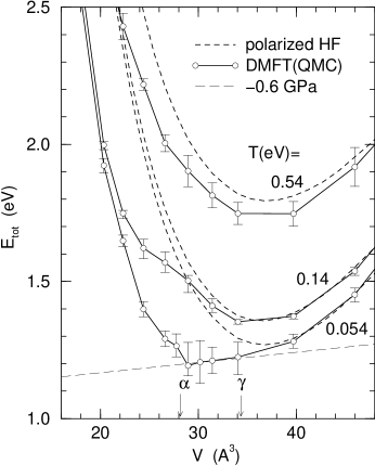
Figure 46: Total LDA+DMFT(QMC) and polarized Hartree–Fock (HF) energy as a function of volume at three temperatures. While the polarized HF energy has one pronounced minimum in the $\gamma$–Ce phase, the LDA+DMFT(QMC) shows a shallowness ($T=0.054,$ eV), which is consistent with the observed $\alpha$-$\gamma$ transition (arrows) within the error bars. These results are also consistent with the experimental pressure given by the negative slope of the dashed line. (from McMahan et al. (2003))

With increasing temperature, the contribution to free energy from the entropy term becomes important. Hence one can look for another signature of the $\alpha\rightarrow\gamma$ transition: the behavior of the entropy. The transition was attributed to rapid increase of the entropy in the region of volumes 28.2-34.4 Å. At large volumes, when spectral weight of the $4f$–electrons is removed from the Fermi level, the entropy saturates at value $k_{B}\mathrm{ln}(2J+1)$, and in the case of the $SU(N)$ approximation assumed in the calculation, the logarithm tends to $\mathrm{ln}(14)$. For smaller volumes the quasiparticle peak grows which causes changes in the specific heat and hence in the entropy through $\int dTC(T)/T$, substantially reducing it to smaller values.

So, the general qualitative picture which comes out from the LDA+DMFT calculations is the following. At large volume ($\gamma$–phase) the $4f$–spectrum is split into Hubbard bands and therefore a local moment is present in the system. With volume reduction a quasiparticle (Abrikosov–Suhl resonance) develops in the vicinity of the Fermi level which causes a drop in the entropy and disappearance of the local moment. Temperature dependence of the quasiparticle peak indicated a substantially larger Kondo temperature in the $\alpha$–phase than in $\gamma$–Ce phase. The obtained results also suggest that $\gamma$- and $\alpha$–phases of Ce are both strongly correlated.

Finally the optical properties of Cerium, were computed both in the alpha and gamma phases by Haule et. al.  Haule et al. (2005). These authors observed that the Kondo collapse and the Mott transition scenario can be differentiated by measuring the optical properties that are controlled by the light electrons, or by studying theoretically the photoemission spectra of the $spd$–electrons. In a Mott transition scenario, the $spd$–electrons are mere spectators, not strongly affected by the localization of the $f$’s. Alternatively, in the Kondo collapse scenario a typical hybridization gap should open up in the $spd$–spectra with a clear optical signature. Their calculation as well as their interpretation of the optical data of Van Der Eb van der Eb et al. (2001) supports the Kondo collapse scenario.

IV.2.2 Plutonium

Many properties of Plutonium have been a long standing puzzle Freeman and Darby (1974). Pu is known to have six crystallographic structures with large variation in their volume Hecker and Timofeeva (2000). Pu shows an enormous volume expansion between $\alpha$- and $\delta$–phases which is about 25%. Within the $\delta$–phase, the system is metallic and has a negative thermal expansion. Transition between $\delta$- and the higher–temperature $\varepsilon$–phase occurs with a 5% volume collapse. Also, Pu shows anomalous resistivity behavior Boring and Smith (2000) characteristic of a heavy fermion systems, but neither of its phases are magnetic, displaying small and relatively temperature independent susceptibility. Photoemission Arko et al. (2000) exhibits a strong narrow Kondo–like peak at the Fermi level consistent with large values of the linear specific heat coefficient, although inverse photoemission experiments have not been done up to now.

Given the practical importance of this material and enormous amount of past experimental and theoretical work, we first review the results of conventional LDA and GGA approaches to describe its properties. Electronic structure and equilibrium properties of Pu were studied earlier by Solovyev et al., 1991; Soderlind et al., 1994 as well as recently by Jones et al., 2000; Savrasov and Kotliar, 2000; Wan and Sun, 2000; Nordstrom et al., 2000; Soderlind, 2001; Soderlind et al., 2002; Kutepov and Kutepova, 2003; Robert, 2004. Using non–magnetic GGA calculations, it was found that the equilibrium volume of its $\delta$–phase is underestimated by 20-30$\%$. The spread in the obtained values can be attributed to different treatments of spin orbit coupling for the 6p semicore states. In particular, the problem was recognized Nordstrom et al. (2000) that many electronic structure methods employ basis sets constructed from scalar–relativistic Hamiltonians and treat spin–orbit interaction variationally Andersen (1975). Within the Pauli formulation (i.e. when only terms up to the order $\frac{1}{c^{2}}$ are kept) the spin–orbit Hamiltonian is given by

$$\frac{2}{rc^{2}}\frac{dV}{dr}\mathbf{\hat{l}\hat{s}},$$ (267)

whose matrix elements are evaluated on the radial solutions of the scalar relativistic version of the Schroedinger’s equation $\phi_{l}(r,E)$ carrying no total (spin+orbit) moment dependence. It has been pointed out Nordstrom et al. (2000) that in the absence of proper evaluations of $\phi_{j=1/2}(r,E_{p^{1/2}})$ $\phi_{j=3/2}(r,E_{p^{3/2}})$ orbitals, one of the options is to neglect the spin–orbital interaction for 6p states completely. This results in the improvement of volume which is of the order of 20% smaller than the experiment as compared to the relativistic Pauli treatment which gives a 30% discrepancy.

One can go beyond the Pauli Hamiltonian and treat the spin–orbital Hamiltonian as an energy–dependent operator Koelling and Harmon (1977).

$$\frac{2}{rc^{2}[1+\frac{1}{c^{2}}(E-V)]^{2}}\frac{dV}{dr}\mathbf{\hat{l}\hat{s}}.$$ (268)

For a narrow band, the energy in the denominator can be taken approximately at the center of the band and the average of the operator can be evaluated without a problem. Our own simulations done with the full potential LMTO method show that the discrepancy in atomic volume is improved from 27% when using Eq. (267) to 21% when using Eq.(268) and appear to be close to the results when the spin–orbit coupling for the 6 p states is neglected. The origin of this improvement lies in a smaller splitting between $6p^{1/2}$ and $6p^{3/2}$ states when incorporating the term beyond $\frac{1}{c^{2}}$.

Models with the assumptions of long range magnetic order have also been extensively explored in the past Solovyev et al. (1991); Soderlind et al. (1994); Savrasov and Kotliar (2000); Wan and Sun (2000); Soderlind (2001); Soderlind et al. (2002); Soderland and Sadigh (2004); Kutepov and Kutepova (2003); Robert (2004). While none of Pu phases are found to be magnetic of either ordered or disordered type Lashley et al. (2004) all existing density functional based calculations predict the existence of long range magnetism. Using GGA and imposing ferromagnetic order, the predictions in the theoretical volumes for the $\delta$–phase have ranged from underestimates by as much as 33% Savrasov and Kotliar (2000) to overestimates by 16% Soderlind et al. (2002). Again, the sensitivity of the results to the treatment of the spin orbit coupling for 6p semicore needs to be emphasized. Our most recent investigation of this problem shows that a 33% discrepancy found with simulation using the Pauli Hamiltonian Savrasov and Kotliar (2000) can be removed if Eq.(268) is utilized. This makes the result consistent with the calculations when spin–orbit coupling for 6p states is completely omitted Soderlind et al. (2002); Robert (2004) or when using fully relativistic calculation Kutepov and Kutepova (2003).

Despite the described inconsistencies between the theory and the experiment for the $\delta$–phase, the volume of the $\alpha$–phase is found to be predicted correctly by LDA Jones et al. (2000); Soderlind (2001); Kutepov and Kutepova (2003) . Since the transport and thermodynamic properties of $\alpha$- and $\delta$–Pu are very similar, the nature of the $\alpha$–phase and the LDA prediction by itself is another puzzle.

Several approaches beyond standard LDA/GGA schemes have been implemented to address these puzzles. The LDA+U method was applied to $\delta$–Pu Bouchet et al. (2000); Savrasov and Kotliar (2000). It is able to produce the correct volume of the $\delta$–phase, for values of the parameter U$\sim$4 eV consistent with atomic spectral data and constrained density functional calculations. However, the LDA+U calculation has converged to the artificial magnetically ordered state. This method is unable to predict the correct excitation spectrum and to recover the $\alpha$–phase. To capture these properties, $U$ must be set to zero. Another approach proposed in the past Eriksson et al. (1999) is the constrained LDA approach in which some of the 5f–electrons, are treated as core, while the remaining electrons are allowed to participate in band formation. Results of the self–interaction–corrected LDA calculations have been also discussed Setty and Cooper (2003); Svane et al. (1999). Recent simulations based on the disordered local moment method Niklasson et al. (2003) have emphasized that the volume of the $\delta$–Pu can be recovered without an assumption of long range magnetic order.

The dynamical mean–field theory offers a way to deal with the problem using the full frequency resolution. Within DMFT the magnetic moments do not need to be frozen and can live at short time scales while giving zero time average values. Also, performing finite temperature calculation ensures that the various orientations of moments enter with proper statistical weights. The LDA+DMFT calculations using Pauli Hamiltonians have been reported in Dai et al. (2003); Savrasov et al. (2001). To illustrate the importance of correlations, the authors Savrasov and Kotliar (2003); Savrasov et al. (2001) discussed the results for various strengths of the on–site Coulomb interaction U. The total energy as a function of volume of the FCC lattice is computed for $T=600$ K using the self–consistent determination of the density in a double iteration loop as described in Section II. The total energy is found to be dramatically different for non–zero $U$ with the possibility of a double minimum for $U^{\prime}s\cong 4$ eV which can be associated with the low volume $\alpha$- and high–volume $\delta$–phases.

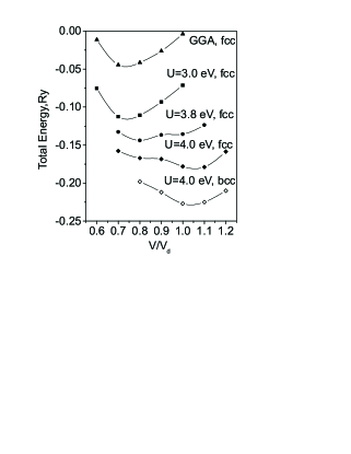
Figure 47: Total energy as a function of volume in Pu for different values of $U$ calculated using the LDA+DMFT approach. Data for the FCC lattice are computed at $T=600$ K, while data for the BCC lattice are given for $T=900$ K.

The calculations for the BCC structure using the temperature $T=900$ K have been also reported Savrasov and Kotliar (2004b). Fig. 47 shows these results for $U=4$ eV with a location of the minimum around $V/V_{\delta}=1.03$. While the theory has a residual inaccuracy in determining the $\delta$- and $\varepsilon$–phase volumes by a few percent, a hint of volume decrease with the $\delta\rightarrow\varepsilon$ transition was clearly reproduced.

The values of $U\sim 4$ eV, which are needed in these simulations to describe the $\alpha\rightarrow\delta$ transition, were found to be in good agreement with the values of on–site Coulomb repulsion between $f$–electrons estimated by atomic spectral data Desclaux and Freeman (1984), constrained density functional studies Turchi et al. (1999), and the LDA+U studies Savrasov and Kotliar (2000).

The double–well behavior in the total energy curve is unprecedented in LDA or GGA based calculations but it is a natural consequence of the proximity to a Mott transition. Indeed, recent studies of model Hamiltonian systems Kotliar et al. (2002) have shown that when the $f$–orbital occupancy is an integer and the electron–electron interaction is strong, two DMFT solutions which differ in their spectral distributions can coexist. It is very natural that allowing the density to relax in these conditions can give rise to the double minima as seen in Fig. 47.

The calculated spectral density of states for the FCC structure using the volume $V/V_{\delta}=0.8$ and $V/V_{\delta}=1.05$ corresponding to the $\alpha$- and $\delta$–phases have been reported  Savrasov et al. (2001); Savrasov and Kotliar (2004b). Fig. 48 compares the results of these dynamical mean–field calculations with the LDA method as well as with the experiment. Fig. 48 (a) shows density of states calculated using LDA+DMFT method in the vicinity of the Fermi level. The solid black line corresponds to the $\delta$–phase and solid grey line corresponds to the $\alpha$–phase. The appearance of a strong quasiparticle peak near the Fermi level was predicted in both phases. Also, the lower and upper Hubbard bands can be clearly distinguished in this plot. The width of the quasiparticle peak in the $\alpha$–phase is found to be larger by 30 percent compared to the width in the $\delta$–phase. This indicates that the low–temperature phase is more metallic, i.e. it has larger spectral weight in the quasiparticle peak and smaller weight in the Hubbard bands. Recent advances have allowed the experimental determination of these spectra, and these calculations are consistent with these measurements Arko et al. (2000). Fig. 48 (b) shows the measured photoemission spectrum for $\delta$- (black line) and $\alpha$–Pu (gray line). A strong quasiparticle peak can clearly be seen. Also a smaller peak located at 0.8 eV is interpreted as the lower Hubbard band. The result of the local density approximation within the generalized gradient approximation is shown in Fig. 48 (a) as a thin solid line. The LDA produces two peaks near the Fermi level corresponding to 5$f^{5/2}$ and 5$f^{7/2}$ states separated by the spin–orbit coupling. The Fermi level falls into a dip between these states and cannot reproduce the features seen in photoemission.

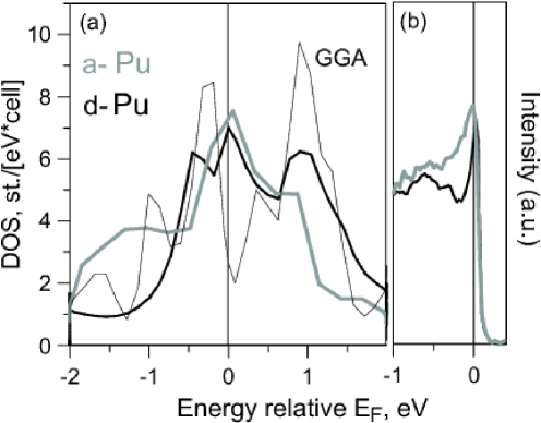
Figure 48: a) Comparison between calculated density of states using the LDA+DMFT approach for FCC Pu: the data for $V/V_{\delta}=1.05,\,U=4.0$ eV (thick black solid line), the data for $V/V_{\delta}=0.80,\,\,U=3.8$ eV (thick gray line) which correspond to the volumes of the $\delta$ and $\alpha$–phases respectively. The result of the GGA calculation (thin solid line) at $V/V_{\delta}=1\,\,(U=0)$ is also given. b) Measured photoemission spectrum of $\delta$ (black line) and $\alpha$ (grey line) Pu at the scale from -1.0 to 0.4 eV (after Ref. Arko et al., 2000).

A newly developed dynamical mean–field based linear response technique  Savrasov and Kotliar (2003) has been applied to calculate the phonon spectra in $\delta$- and $\varepsilon$–Pu Dai et al. (2003). Self–energy effects in the calculation of the dynamical matrix have been included using the Hubbard I approximation Hubbard (1963). A considerable softening of the transverse phonons is observed around the $L$ point in the calculated frequencies as a function of the wave vector along high–symmetry directions in the Brillouin zone for the $\delta$–phase (see Fig. 49) This indicates that the $\delta$–phase may be close to an instability with a doubling of the unit cell. Another anomaly is seen for the transverse acoustic mode along (011) which is connected to the non–linear behavior of the lowest branch at small $q$. Overall, the phonon frequencies are positive showing the internal stability of the positions of the nuclear coordinates in $\delta$–Pu.

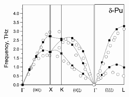
Figure 49: Calculated phonon spectrum of $\delta$–Pu (squares connected by full lines) in comparison with experiment (open circles Wong et al. (2003))

Remarkably, the experiment Wong et al. (2003) which came out after the publication  Dai et al. (2003) has confirmed these theoretical predictions. The measured points are shown on top of the calculated curves in Fig. 49.

The presented results allow us to stress that, in spite of the various approximations and their respective shortcomings discussed in the text, it is clear that LDA+DMFT is a most promising technique for studying volume collapse transition phenomena. Besides the satisfying agreement with experiment (given the crudeness of various approximations) both the studies of Plutonium and Cerium have brought in a somewhat unexpected view point for the electronic structure community. The delocalized phase ($\alpha$–Plutonium and $\alpha$–Cerium) are not weakly correlated, in spite of the success of density functional theory in predicting their volume and elastic properties.

IV.3 Systems with local moments

The magnetism of metallic systems has been studied intensively Moriya (1985). Metallic ferromagnets range from being very weak with a small magnetization to very strong with a saturated magnetization close to the atomic value. For a review of early theories see e.g. Refs. Herring (1966); Vonsovsky (1974); Moriya (1985). Weak ferromagnets are well described by spin density wave theory, where spin fluctuations are localized in a small region of momentum space. Quantitatively they are well described by LSDA. The ferromagnetic to paramagnetic transition is driven by amplitude fluctuations. In strong ferromagnets, there is a separation of time scales. $\hbar/t$ is the time scale for an electron to hop from site to site with hopping integral $t$, which is much shorter than $\hbar/J,$ the time scale for the moment to flip in the paramagnetic state. The spin fluctuations are localized in real space and the transition to the paramagnetic state is driven by orientation fluctuations of the spin. The exchange splitting $J$ is much larger than the critical temperature.

Obtaining a quantitative theory of magnetic materials valid both in the weak and strong coupling regime, both above and below the Curie temperature, has been a theoretical challenge for many years. It has been particularly difficult to describe the regime above $T_{c}$ in strong ferromagnets when the moments are well formed but their orientation fluctuates. A related problem arises in magnetic insulators above their ordering temperature, when this ordering temperature is small compared to electronic scales. This is a situation that arises in transition metal monoxides (NiO and MnO) and led to the concept of a Mott insulator. In these materials the insulating gap is much larger than the Néel temperature. Above the ordering temperature, we have a collection of atoms with an open shell interacting via superexchange. This is again a local moment regime which cannot be accessed easily with traditional electronic structure methods.

Two important approaches were designed to access the disordered local moment (DLM) regime. One approach Hubbard (1979a, b, 1981) starts form a Hubbard like Hamiltonian and introduces spin fluctuations via the Hubbard–Stratonovich transformation Stratonovich (1958); Wang et al. (1969); Evenson et al. (1970); Cyrot (1970) which is then evaluated using a static coherent potential approximation (CPA) and improvements of this technique. A dynamical CPA Al-Attar and Kakehashi (1999) was developed by Kakehashi Kakehashi (1992); Kakehashi et al. (1998); Kakehashi (2002) and is closely related to the DMFT ideas. A second approach begins with solutions of the Kohn–Sham equations of a constrained LDA approximation in which the local moments point in random directions, and averages over their orientation using the KKR–CPA approach Gyorffy and Stocks (1979); Faulkner (1982). The average of the Kohn–Sham Green’s functions then can be taken as the first approximation to the true Green’s functions, and information about angle resolved photoemission spectra can be extracted Gyorffy et al. (1985); Staunton et al. (1985). There are approaches that are based on a picture where there is no short range order to large degree. The opposite point of view, where the spin fluctuations far away form the critical temperature are still relatively long ranged was put forward in the fluctuation local band picture Capellmann (1974); Korenman et al. (1977a, b, c); Prange and Korenman (1979b, a).

To describe the behavior near the critical point requires renormalization group methods, and the low–temperature treatment of this problem is still a subject of intensive research Belitz and Kirkpatrick (2002). There is also a large literature on describing ferromagnetic metals using more standard many–body methods Liebsch (1981); Tréglia et al. (1982); Manghi et al. (1997, 1999); Nolting et al. (1987); Steiner et al. (1992).

While the density functional theory can in principle provide a rigorous description of the thermodynamic properties, at present there is no accurate practical implementation available. As a result, the finite–temperature properties of magnetic materials are estimated following a simple suggestion Liechtenstein et al. (1987). Constrained DFT at $T=0$ is used to extract exchange constants for a classical Heisenberg model, which in turn is solved using approximate methods (e.g. RPA, mean–field) from classical statistical mechanics of spin systems Liechtenstein et al. (1987); Rosengaard and Johansson (1997); Halilov et al. (1998); Antropov et al. (1996). The most recent implementation of this approach gives good values for the transition temperature of Iron but not of Nickel Pajda et al. (2001). However it is possible that this is the result of not extracting the exchange constants correctly, and a different algorithm for carrying out this procedure was proposed Bruno (2003).

DMFT can be used to improve the existing treatments of DLM to include dynamical fluctuations beyond the static approximation. Notice that single–site DMFT includes some degree of short range correlations. Cluster methods can be used to go beyond the single–site DMFT to improve the description of short range order on the quasiparticle spectrum. DMFT also allows us to incorporate the effects of the electron–electron interaction on the electronic degrees of freedom. This is relatively important in metallic systems such as Fe and Ni and absolutely essential to obtain the Mott–Hubbard gap in transition metal monoxides.

The dynamical mean–field theory offers a very clear description of the local moment regime. Mathematically, it is given by an effective action of a degenerate impurity model in a bath which is sufficiently weak at a given temperature to quench the local moment. This bath obeys the DMFT self–consistency condition. If one treats the impurity model by introducing the Hubbard–Stratonovich field and treats it in a static approximation, one obtains very simple equations as those previously used to substantiate the DLM picture.

IV.3.1 Iron and Nickel

Iron and Nickel were studied in Refs. Katsnelson and Lichtenstein, 2000; Lichtenstein et al., 2001. The values $U=2.3$ $(3.0)$ eV for Fe (Ni) and interatomic exchange of $J=0.9$ eV for both Fe and Ni were used, as obtained from the constrained LDA calculations Bandyopadhyay and Sarma (1989); Anisimov et al. (1997a); Lichtenstein and Katsnelson (1997, 1998). These parameters are consistent with those of many earlier studies and resulted in a good description of the physical properties of Fe and Ni. In Ref. Lichtenstein et al., 2001 the general form of the double counting correction $V_{\sigma}^{DC}=\frac{1}{2}Tr_{\sigma}\mathcal{M}_{\sigma}(0)$ was taken. Notice that because of the different self–energies in the $e_{g}$ and $t_{2g}$ blocks the DMFT Fermi surface does not coincide with the LDA Fermi surface.

The LDA+U method, which is the static limit of the LDA+DMFT approach, was applied to the calculation of the magnetic anisotropy energies Imseok et al. (2001). This study revealed that the double counting correction induces shifts in the Fermi surface which brings it in closer agreement with the De Haas Van Alphen experiments. The values of $U$ used in this LDA+U work are slightly lower than in the DMFT work, which is consistent with the idea that DMFT contains additional screening mechanisms, not present in LDA+U. This can be mimicked by a smaller value of the interaction $U$ in the LDA+U calculation. However, the overall consistency of the trends found in the LDA+U and the DMFT studies are very satisfactory.

More accurate solutions of the LDA+DMFT equations have been presented as well. The impurity model was solved by QMC in Ref.  Lichtenstein et al., 2001 and by the FLEX scheme in Ref. Katsnelson and Lichtenstein, 2002. It is clear that Nickel is more itinerant than Iron (the spin–spin autocorrelation decays faster), which has longer lived spin fluctuations. On the other hand, the one–particle density of states of Iron closely resembles the LSDA density of states while the DOS of Nickel, below $T_{c}$, has additional features which are not present in the LSDA spectra Iwan et al. (1979); Eberhardt and Plummer (1980); Altmann et al. (2000): the presence of the famous 6 eV satellite, the 30% narrowing of the occupied part of $d$–band and the 50% decrease of exchange splittings compared to the LDA results. Note that the satellite in Ni has substantially more spin–up contributions in agreement with photoemission spectra Altmann et al. (2000). The exchange splitting of the $d$–band depends very weakly on temperature from $T=0.6T_{C}$ to $T=0.9T_{C}$. Correlation effects in Fe are less pronounced than in Ni due to its large spin splitting and the characteristic BCC structural dip in the density of states for the spin–down states near the Fermi level, which reduces the density of states for particle–hole excitations.

The uniform spin susceptibility in the paramagnetic state, ${\chi}_{q=0}=dM/dH$, was extracted from the QMC simulations by measuring the induced magnetic moment in a small external magnetic field. It includes the polarization of the impurity Weiss field by the external field Georges et al. (1996). The dynamical mean–field results account for the Curie–Weiss law which is observed experimentally in Fe and Ni. As the temperature increases above $T_{c}$, the atomic character of the system is partially restored resulting in an atomic like susceptibility with an effective moment $\mu_{eff}$. The temperature dependence of the ordered magnetic moment below the Curie temperature and the inverse of the uniform susceptibility above the Curie point are plotted in Fig. 50 together with the corresponding experimental data for Iron and Nickel Wolfarth (1986). The LDA+DMFT calculation describes the magnetization curve and the slope of the high–temperature Curie–Weiss susceptibility remarkably well. The calculated values of high–temperature magnetic moments extracted from the uniform spin susceptibility are $\mu_{eff}=3.09$ $(1.50)\mu_{B}$ for Fe (Ni), in good agreement with the experimental data $\mu_{eff}=3.13$ $(1.62)\mu_{B}$ for Fe (Ni) Wolfarth (1986).

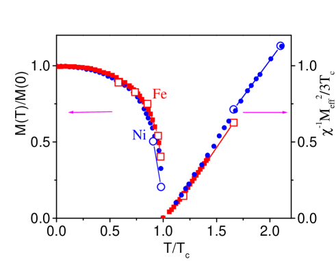
Figure 50: Temperature dependence of ordered moment and the inverse ferromagnetic susceptibility for Fe (open square) and Ni (open circle) compared with experimental results for Fe (square) and Ni (circle) (from Ref. Stocks et al., 1998). The calculated moments were normalized to the LDA ground state magnetization (2.2 $\mu_{B}$ for Fe and 0.6 $\mu_{B}$ for Ni).

The Curie temperatures of Fe and Ni were estimated from the disappearance of spin polarization in the self–consistent solution of the DMFT problem and from the Curie–Weiss law. The estimates for $T_{C}=1900$ $(700)$ K are in reasonable agreement with experimental values of $1043$ $(631)$ K for Fe (Ni) respectively Wolfarth (1986), considering the single–site nature of the DMFT approach, which is not able to capture the reduction of $T_{C}$ due to long–wavelength spin waves. These effects are governed by the spin–wave stiffness. Since the ratio of the spin–wave stiffness $D$ to $T_{C}$, $T_{C}$/$a^{2}D,$ is nearly a factor of 3 larger for Fe than for Ni Wolfarth (1986) ($a$ is the lattice constant), we expect the $T_{C}$ in DMFT to be much higher than the observed Curie temperature in Fe than in Ni. Quantitative calculations demonstrating the sizeable reduction of $T_{C}$ due to spin waves in Fe in the framework of a Heisenberg model were performed in Ref. Pajda et al., 2001. This physics whereby the long wavelength fluctuations renormalize the critical temperature would be reintroduced in the DMFT using E–DMFT. Alternatively, the reduction of the critical temperature due to spatial fluctuations can be investigated with cluster DMFT methods.

The local susceptibility is easily computed within the DMFT–QMC. Its behavior as a function of temperature gives a very intuitive picture of the degree of correlations in the system. In a weakly correlated regime we expect the local susceptibility to be nearly temperature independent, while in a strongly correlated regime we expect a leading Curie–Weiss behavior at high temperatures $\chi_{local}=\mu_{loc}^{2}/({3}T+const.)$ where $\mu_{loc}$ is an effective local magnetic moment. In the Heisenberg model with spin $S$, $\mu_{loc}^{2}=S(S+1)g_{s}^{2}$ and for the well–defined local magnetic moments (e.g., for rare–earth magnets) this quantity should be temperature independent. For the itinerant electron magnets, $\mu_{loc}$ is temperature–dependent due to a variety of competing many–body effects such as Kondo screening, the induction of local magnetic moment by temperature Moriya (1985) and thermal fluctuations which disorder the moments Irkhin and Katsnelson (1994). All these effects are included in the DMFT calculations.

The comparison of the values of the local and the $q=0$ susceptibility gives a crude measure of the degree of short–range order which is present above $T_{C}$. As expected, the moments extracted from the local susceptibility are a bit smaller (2.8  $\mu_{B}$ for Iron and 1.3  $\mu_{B}$ for Nickel) than those extracted from the uniform magnetic susceptibility. This reflects the small degree of the short–range correlations which remain well above $T_{C}$ Mook and Lynn (1985). The high–temperature LDA+DMFT clearly shows the presence of a local moment above $T_{C}$. This moment is correlated with the presence of high–energy features (of the order of the Coulomb energies) in the photoemission. This is also true below $T_{C}$, where the spin dependence of the spectra is more pronounced for the satellite region in Nickel than for that of the quasiparticle bands near the Fermi level. This can explain the apparent discrepancies between different experimental determinations of the high–temperature magnetic splittings Kisker et al. (1984); Kakizaki et al. (1994); Sinkovic et al. (1997); Kreutz et al. (1989) as being the results of probing different energy regions. The resonant photoemission experiments Sinkovic et al. (1997) reflect the presence of local–moment polarization in the high–energy spectrum above the Curie temperature in Nickel, while the low–energy ARPES investigations Kreutz et al. (1989) results in non–magnetic bands near the Fermi level. This is exactly the DMFT view on the electronic structure of transition metals above $T_{C}$. Fluctuating moments and atomic–like configurations are large at short times, which results in correlation effects in the high–energy spectra such as spin–multiplet splittings. The moment is reduced at longer time scales, corresponding to a more band–like, less correlated electronic structure near the Fermi level.

IV.3.2 Classical Mott insulators

NiO and MnO represent two classical Mott–Hubbard systems (in this section we shall not distinguish between Mott–Hubbard insulators and charge transfer insulators Zaanen et al. (1985)). Both materials are insulators with the energy gap of a few eV regardless whether they are antiferromagnetic or paramagnetic. The spin–dependent LSDA theory strongly underestimates the energy gap in the ordered phase. This can be corrected by the use of the LDA+U method. Both theories however fail completely to describe the local moment regime reflecting a general drawback of band theory to reproduce the atomic limit. Therefore the real challenge is to describe the paramagnetic insulating state where the self–energy effects are crucial both for the electronic structure and for recovering the correct phonon dispersions in these materials. The DMFT calculations have been performed Savrasov and Kotliar (2003) by taking into account correlations among $d$–electrons. In the regime of large $U$, adequate for both for NiO and MnO in the paramagnetic phase, the correlations were treated within the well–known Hubbard I approximation.

The calculated densities of states using the LDA+DMFT method for the paramagnetic state of NiO and MnO Savrasov and Kotliar (2003) have revealed the presence of both lower and upper Hubbard sub–bands. These were found in agreement with the LDA+U calculations of Anisimov Anisimov et al. (1991) which have been performed for the ordered states of these oxides. Clearly, spin integrated spectral functions do not show an appreciable dependence with temperature and look similar below and above phase transition point.

The same trend is known to be true for the phonon spectra which do not depend dramatically on magnetic ordering since the Néel temperatures in these materials are much lower of their energy gaps. Fig. 51 shows phonon dispersions for NiO along major symmetry directions. A good agreement with experiment Roy et al. (1976) can be found for both acoustic and transverse modes. A pronounced softening of the longitudinal optical mode along both $\Gamma X$ and $\Gamma L$ lines is seen at the measured data which is in part captured by the theoretical DMFT calculation: the agreement is somewhat better along the $\Gamma X$ direction while the detailed $q$–dependence of these branches shows some residual discrepancies.

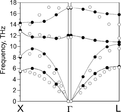
Figure 51: Comparison between calculated using the DMFT method (filled circles) and experimental (open circles) phonon dispersion curves for NiO.

The results of these calculations have been compared with the paramagnetic LDA, as well as with the antiferromagnetic LSDA and LSDA+U solutions in Ref. Savrasov and Kotliar, 2003. The paramagnetic LDA did not reproduce the insulating behavior and therefore fails to predict the splitting between the LO and TO modes. Due to metallic screening, it underestimates the vibrations for NiO and predicts them to be unstable for MnO. The spin resolved LSDA solution imposes the existence of long–range magnetic order and is an improvement, but strongly underestimates the energy gap. As a result, an apparent underestimation of the longitudinal optical modes has been detected Savrasov and Kotliar (2003). On the other hand, the calculations with correlations produce much better results. This is found both for the LSDA+U and the LDA+Hubbard I calculations which can be interpreted as good approximations to the DMFT solutions for the ordered and disordered magnetic states. Such an agreement can be related with the fact that the direct $d-d$ gap is fixed by $U$, and the charge transfer gap comes out better in the theory. Thus, the local screening of charge fluctuations are treated more appropriately.

IV.4 Other applications

DMFT concepts and techniques are currently being applied to investigate a broad range of materials and a wide variety of strong correlation problems. This is a very active research frontier, comprising topics as diverse as manganites, ruthenates, vanadates, actinides, lanthanides, Buckminster fullerenes, quantum criticality in heavy fermion systems, magnetic semiconductors, actinides, lanthanides, Bechgaard salts, high–temperature superconductors, as well as surfaces heterostructures alloys and many other types of materials. We mention below a small subset of the systems under investigation using the techniques described in this review, just in order to give the reader a glimpse of the breadth of this rapidly developing field and the great potential of DMFT methods to investigate strongly correlated materials. For earlier reviews see Ref. Held et al., 2001c and also Held et al. (2003), Lichtenstein et al. (2002b) and Lichtenstein et al. (2002a); Kotliar and Savrasov (2001); Georges (2004a, b); Kotliar and Vollhardt (2004); Kotliar (2005).

Transition Metal Oxides
$\bullet$ A large body of DMFT studies focused on the Manganites with the perovskite structure, like La_1-xCa_xMnO₃ or La_1-xSr_xMnO₃. These materials attracted attention because of their “colossal” magnetoresistance, which is an extreme sensitivity of resistance to an applied magnetic field Tokura (2003, 1990); Dagotto (2002). The phase diagram of these materials in the temperature composition plane is very rich, displaying ferromagnetism, antiferromagnetism, and charge and orbital ordering. Several physical mechanism and various interactions are important in these materials such as the double exchange mechanism (i.e. the gain in kinetic energy of the $e_{g}$ electrons when the $t_{2g}$ electrons are ferromagnetically aligned), the coupling of the $e_{g}$ electrons to Jahn–Teller modes (i.e. distortions of the Oxygen octahedra which lift the cubic degeneracy of the $e_{g}$ orbitals) and breathing Oxygen phonon modes. These materials, as well as the copper oxides, also spurred new studies on strong electron-phonon coupling problems and their interplay with the electron electron interactions. Semiclassical treatments of the core spins and the phonons, help to dramatically simplify the solution of the DMFT equations.

For various DMFT studies of the electron phonon coupling problem in the manganites see Furukawa (1994); Millis et al. (1996b); Phan and Tran (2003); Fishman and Jarrell (2002); Fishman and Jarrell (2003a, b); Chernyshev and Fishman (2003); Izyumov Yu and Letfulov (2001); Michaelis and Millis (2003); Held and Vollhardt (2000); Imai and Kawakami (2000); Tran (2003); Ciuchi and De Pasquale (1999); Blawid et al. (2003); Pankov et al. (2002); Deppeler and Millis (2002b, a); Fratini et al. (2001, 2000); Ciuchi et al. (1997); Benedetti and Zeyher (1999); Venketeswara Pai et al. (2003); Ramakrishnan et al. (2003, 2004).

$\bullet$ High-temperature superconductivity The discovery of high-temperature superconductivity in the cuprates posed the great theoretical and computational challenge of uncovering the mechanism of this phenomena, which is still not sufficiently understood to this day. The cluster extensions of DMFT are actively being applied in an effort to further unravel the mystery of the high-temperature superconductivity Civelli et al. (2005); Katsnelson and Lichtenstein (2000); Dahnken et al. (2005, 2004); Potthoff et al. (2003); Maier et al. (2005); Macridin et al. (2005); Maier et al. (2004b); Macridin et al. (2004); Maier et al. (2002b); Aryanpour et al. (2002); Huscroft et al. (2001); Maier et al. (2000a).

$\bullet$ Other transition-metal oxides have recently been studied with DMFT. Na_xCoO₂ has received much interest due to anomalous thermoelectric properties in addition to superconductivity upon hydration.  Ishida et al. (2005); Lechermann et al. (2005b); Saha-Dasgupta et al. (2005b). LiVO₂ displays an unusually large effective mass for a $d$-electron system, which gave rise to the idea that this may be an example of a heavy-fermion $d$-electron material  Nekrasov et al. (2003). TiOCl displays $1d$ orbital ordering at low temperatures, and exhibits a spin-Peierls transition  Seidel et al. (2003); Saha-Dasgupta et al. (2005a); Hoinkis et al. (2005). Ca_2-xSr_xRuO₄ attracted a lot of attention as it exhibits unconventional $p$–wave superconductivity at low temperatures, a Mott transition, and a surface-sensitive spectra Liebsch and Lichtenstein (2000b); Anisimov et al. (2002); Liebsch (2003b, a); Lichtenstein and Liebsch (2002).

Organic Materials and Supramolecular Structures
$\bullet$ Fullerines K_nC₆₀. The doped Buckminster fullerenes are solids formed from $C_{60}$ – a molecule shaped like a soccer ball – with the alkali metal sitting in the middle. Their proximity to the Mott transition was pointed out by Gunnarsson, 1997. At low temperatures K₃C₆₀ is an $s$–wave superconductor, where both the strong electron–phonon interaction and the Coulomb repulsion need to be taken into account. DMFT has been helpful in understanding the transition to superconductivity  Capone et al. (2002a); Han et al. (2003); Capone et al. (2000); Capone et al. (2002b). A Mott insulating state has also been realized recently in another nanostructured supercrystal family, that of potassium loaded zeolites, and realistic DMFT calculations have been carried out  Arita et al. (2004).

$\bullet$ Bechgaard salts Vescoli et al. (2000); Biermann et al. (2001). In addition to the quasi-two dimensional organic compounds of the kappa and theta families mentioned in section IV, there have been chain-DMFT studies of $(TMTTF)_{2}X$ and $(TMTSF)_{2}X$. These are strongly anisotropic materials made of stacks of organic molecules. Their optical properties are very unusual. At high temperatures the electrons move mainly along the chains, before undergoing inelastic collisions forming a “Luttinger liquid” – one of the possible states of the one–dimensional electron gas. By contrast, at sufficiently low temperatures the electronic structure becomes effectively three–dimensional. For example, they exhibit a very narrow Drude peak carrying only one percent of the total optical weight  Vescoli et al. (2000); Biermann et al. (2001). Investigations of the unusual properties of these materials, and in particular of the crossover between the low- and high–temperature regimes, using cluster generalizations of DMFT have been performed in Refs.  Vescoli et al., 2000; Biermann et al., 2001. Other aspects have recently been addressed in Refs. Georges et al., 2000; Giamarchi et al., 2004.

Heavy Fermion Systems and Silicides
$\bullet$ Heavy fermion materials are compounds containing both $f$–electrons and lighter $s,p,d$–electrons. They can form a “heavy” Fermi liquid state at low temperatures where the quasiparticles are composites of $f$–electron spins and conduction electron charges, or can order antiferromagnetically at low temperatures (for recent review see Stewart (2001)).

The boundary between the Fermi liquid and the itinerant antiferromagnet has been a subject of intensive theoretical and experimental study. Recent neutron scattering experiments are consistent with a local spin self–energy, and have motivated an extended dynamical mean–field descriptions of the Kondo lattice model  Si (2001); Si et. al. et al. (1999); Si et al. (2001); Jian-Xin et al. (2003); Grempel and Si (2003); Ingersent and Si (2002); Si et al. (2003) which reproduces many features of the experiment at zero temperature. For a recent discussion see  Si (2003). A corresponding study of Anderson lattice model Sun and Kotliar (2003) suggests that nonlocal effects, which require a cluster dynamical mean–field study, play an important role.

An interesting issue is whether the optical sum rule, integrated up to some cutoff of the order of one eV, can be a strong function of temperature in heavy fermion insulators. The $f$–sum rule states that if the integration is performed up to infinite frequency, the result is temperature independent. In most materials, this sum rule is obeyed even when a finite upper limit of the order of an electronic energy is used. This was found in Ce₃Bi₄Pt₃ Bucher et al. (1994) and in FeSi  Schlesinger et al. (1993)) Urasaki and Saso (2000); Smith et al. (2003); van der Marel (2003). In Ref. Damascelli, 1999, it has been shown that the integrated optical weight up to 0.5 eV is a strong function of temperature, and if an insulating gap much smaller than the cutoff is open, spectral weight is transferred to very high frequencies. This problem was theoretically addressed using single–site DMFT applied to the Anderson lattice model, and the theory supports a gradual filling of the gap without area conservation  Rozenberg et al. (1995). More recent studies applied to a multiband Hubbard model Urasaki and Saso (2000); Smith et al. (2003); van der Marel (2003) and to the Anderson lattice Vidhyadhiraja et al. (2003) yield excellent quantitative agreement with the most recent experiments. Of great interest is the behavior of these materials in an external field, which is easily incorporated into the DMFT equations  Meyer and Nolting (2001); de’ Medici et al. (2005b).One interesting phenomena is the possibility of metamagnetism, namely the anomalous increase of the magnetization and the concomitant changes in electronic structure as a function of external field, known as a metamagnetic transition. This is displayed in many heavy fermion systems such as CeRu₂Si₂. An important issue is whether a transition between a state with a large Fermi surface and a small Fermi surface takes place as a function of magnetic field.

Inhomogeneous Systems
$\bullet$ Magnetic semiconductors are materials where the magnetization is strongly tied to the carrier concentration. They offer the possibility of controlling the charge conductivity (as in the usual semiconductors) and the spin conductivity (by controlling the magnetization), by varying the carrier concentration. Great excitement in this field has been generated by the discovery of high–temperature ferromagnetism in these materials Vollhardt et al. (1999); Kübler (2000); Kuebler (2002). A main challenge is to understand the strong dependence of the magnetization on the carrier concentration of the magnetic atoms and on the concentration of the conduction electrons or holes. This problem is closely related to the Anderson lattice model and several DMFT studies of this problem have appeared Chattopadhyay et al. (2001); Das Sarma et al. (2003). DMFT has been successfully applied to half magnets such as NiMnSb  Chioncel et al. (2003a); Chioncel et al. (2005); Irkhin et al. (2004) as well as magnetic multilayers Chioncel and Lichtenstein (2004). For a recent DMFT study of the dependence of the critical temperature on various physical parameters see Moreno et al. (2005).

$\bullet$ Strongly inhomogeneous systems: systems near an Anderson transition. The dynamical mean–field theory has been formulated to accommodate strongly inhomogeneous situations such as systems near an Anderson transition, by allowing an arbitrary site dependence of the Weiss field Dobrosavljevic and Kotliar (1997). Recent progress in simplifying the analysis and solution of these equations was achieved using the typical medium approach of Dobrosavljevic et al. Dobrosavljec et al. (2003). The statistical DMFT approach can also be used to study the interplay of disorder and the electron–phonon coupling Bronold and Fehske (2003).

$\bullet$ Heterostructures surfaces and interfaces

Another application of DMFT is to study correlation effects on surfaces, which likely to be more pronounced than in the bulk Okamoto and Millis (2004b); Okamoto and Millis (2004c, d); Freericks (2004). For an early discussion of these effects see Refs. Sawatzky, 1995; Hesper et al., 2000. DMFT equations for the study of correlation effects on surfaces and surfaces phase transitions were written down by Potthoff and collaborators  Potthoff and Nolting (1999c, a, b). and successfully applied to study the Mott transition on surfaces by Perfetti et al. (2003); Liebsch (2003c). DMFT has been applied to inhomogeneous situations involving a much longer periodicity. These studies were motivated by the discovery of stripes in high–temperature superconductors.

V Outlook

Dynamical mean–field methods represent a new advance in many–body physics. They provide an excellent description of the strongly correlated regime of many three–dimensional transition–metal oxides, which had not been accessible to other techniques. Additionally, DMFT has given new insights into strongly correlated electron systems near a metal–insulator transition, or localization–delocalization boundary.

The combination of advanced electronic structure methods with the dynamical mean–field technique has already resulted in new powerful methods for modeling correlated materials. Further improvements are currently being pursued, as the implementations of GW methods and dynamical mean–field ideas Aryasetiawan and Gunnarsson (1998); Zein and Antropov (2002); Sun and Kotliar (2002, 2004); Biermann et al. (2003).

In the field of statistical mechanics, the development of mean–field theories was followed up by the development of renormalization group approaches incorporating the physics of long wavelength fluctuations which become dominant near critical points. The development of effective renormalization techniques for correlated electrons and electronic structure applications is a major challenge ahead. It will allow for more accurate derivation of low–energy Hamiltonians, and improve the solution of model Hamiltonians beyond the dynamical mean–field theory based on small clusters.

The forces acting on the atoms have been recently evaluated in the realistic DMFT treatment of phonons in correlated electron systems Savrasov and Kotliar (2003); Dai et al. (2003). The indications that DMFT captures correctly the forces on the atoms in correlated materials bodes well for combining this development with molecular dynamics to treat the motion of ions and electrons simultaneously. This remains one of the great challenges for the future.

In conclusion, DMFT is a theory which can accurately capture local physics. We emphasize that the notion of local is flexible, and generically refers to some predefined region in which correlations are treated directly (e.g. a single–site, or a cluster of sites). Current computational limitations restrict the local region to be a relatively small number of sites for lattice models. Despite this restriction, DMFT and its cluster extensions have been very successful in describing a wide variety of materials properties where conventional techniques such as LDA have failed. Therefore, it seems that there finally exists a general tool which can accurately treat many of the problems posed by strong correlation in realistic materials. With the increasing number of realistic DMFT implementations and studies of materials, more detailed comparisons with experiments will emerge. Ultimately, this experience will allow us to understand which aspects of the strong correlation problem lie within the scope of the method, and which aspects require the treatment of non–Gaussian, long wavelength fluctuations of collective modes not included in the approach.

Appendix A Derivations for the QMC section

Derivation of Eq. (216)

First, we show that

$$\text{Tr}_{{d^{\dagger},d}}\left(\prod_{1\leq k\leq K}e^{d^{\dagger}A^{(k)}d}\right)=\det\left(1+\prod_{1\leq k\leq K}e^{A^{(k)}}\right)$$ (269)

where $d_{i}$ ($1\leq i\leq n$) are fermionic operators, $A^{(k)}$ ($1\leq k\leq K$) $n\times n$ matrices, and the notation $d^{\dagger}A^{(k)}d\equiv\sum_{1\leq i,j\leq n}d^{\dagger}_{i}A^{(k)}_{ij}d_{j}$. Indeed using

$$\left[d^{\dagger}Ad,d^{\dagger}Bd\right]=d^{\dagger}\left[A,B\right]d$$ (270)

and Baker–Campbell–Hausdorff formula $e^{A}e^{B}=e^{M}$ with

$$M\equiv A+B+\frac{1}{2}[A,B]+a_{2}[A,[A,B]]+\dots$$ (271)

we have

$$\exp(d^{\dagger}Ad)\exp(d^{\dagger}Bd)=\exp(d^{\dagger}Md)$$

By recursion, this generalizes to $K$ matrices, so we just have to prove the result for $K=1$, $A^{(1)}=M$. If $M$ is diagonal, the result is straightforward. For a general matrix $M$, by directly expanding the exponential of the left hand side and using Wick theorem, we see that $\text{Tr}_{{d^{\dagger},d}}e^{d^{\dagger}Md}$ is a series in $\text{Tr}M^{k}$ ($k\geq 0$) and is therefore invariant under any change of basis, and therefore $\det(1+e^{M})$. Hence the result follows by diagonalizing $M$.

Second, we use the determinant formula

$$\begin{vmatrix}1&0&\dots&0&B_{L}\\ -B_{1}&1&\dots&\dots&0\\ 0&-B_{2}&1&\dots&\dots\\ \dots&\dots&\dots&1&0\\ \dots&\dots&\dots&-B_{L-1}&1\\ \end{vmatrix}=\det(1+B_{L}B_{L-1}\dots B_{1})$$

where $B_{1},\dots,B_{L}$ are $n\times n$ matrices. This formula results by recursion from the general formula for block matrices:

$$\det\begin{pmatrix}A&B\\ C&D\end{pmatrix}= \det\left[\begin{pmatrix}1&B\\ 0&D\end{pmatrix}\begin{pmatrix}A-BD^{-1}C&0\\ D^{-1}C&1\end{pmatrix}\right]$$

$$= \det D\det(A-BD^{-1}C)$$ (272)

Derivation of Eq.(217)

The first step is to obtain an explicit formula for $g_{\{S\}}$ Blankenbecler et al. (1981). A quick way is to replace $a_{p\mu}$ and $a_{p\nu}^{\dagger}$ in the trace by $\exp(\psi^{\dagger}\Lambda^{\dagger}_{\mu}a)$ and $\exp(a^{\dagger}\Lambda_{\nu}\psi)$, where $\psi$ is an auxiliary fermion and $(\Lambda_{\mu})_{ij}=\lambda\delta_{j0}\delta_{i\mu}$ where $0$ is the index of $\psi$. Starting from the explicit trace expression of the Green’s function, distinguishing the cases $l_{1}\geq l_{2}$ and $l_{1}<l_{2}$, using Eq. (269) and Eq. (A), we finally expand to second order in $\lambda$ and obtain (see also Georges et al. (1996) ):

$$g_{\{S\}}^{\sigma}(l_{1},l_{2})=\begin{cases}B^{\sigma}_{l_{1}-1}\dots B^{\sigma}_{l_{2}}\bigl{(}1+B^{\sigma}_{l_{2}-1}\dots B^{\sigma}_{1}B^{\sigma}_{L}\dots B^{\sigma}_{l_{2}}\bigr{)}^{-1}&\text{ for }l_{1}\geq l_{2}\\ -B^{\sigma}_{l_{1}-1}\dots B^{\sigma}_{1}B^{\sigma}_{L}\dots B^{\sigma}_{l_{2}}\bigl{(}1+B^{\sigma}_{l_{2}-1}\dots B^{\sigma}_{1}B^{\sigma}_{L}\dots B^{\sigma}_{l_{2}}\bigr{)}^{-1}&\text{ for }l_{1}<l_{2}\end{cases}$$ (273)

A straightforward calculation then shows that $g_{{\{S\}}}^{\sigma}{\cal O}_{\sigma}(\{S\})=1$.

Derivation of Eq.(219)

Equation (219) follows from the observation that ${\cal O}_{\sigma}(\{S\})\prod_{i=n}^{1}e^{-\widetilde{{\cal V}}^{i\sigma}(\{S\})}$ depends on the configuration $\{S\}$ only on its diagonal blocks, which leads to

$${\cal O}_{\sigma}(\{S\})\prod_{i=n}^{1}e^{-\widetilde{{\cal V}}^{i\sigma}(\{S\})}-{\cal O}_{\sigma}(\{S^{\prime}\})\prod_{i=n}^{1}e^{-\widetilde{{\cal V}}^{i\sigma}(\{S^{\prime}\})}=\\ \prod_{i=n}^{1}e^{-\widetilde{{\cal V}}^{i\sigma}(\{S\})}-\prod_{i=n}^{1}e^{-\widetilde{{\cal V}}^{i\sigma}(\{S^{\prime}\})}$$ (274)

which yields Eq. (219).

Derivation of the fast update formula (224)

We present here the steps to go from Eq. (224) to Eq. (225). Since the difference between the two $V$ is in the $l$ block, $A_{\sigma}$ has the form

$$A_{\sigma}=\begin{pmatrix}1&0&\dots&A^{\sigma}_{1l}&\dots&0\\ 0&1&\dots&A^{\sigma}_{2l}&\dots&0\\ \vdots&\vdots&\vdots&\vdots&\vdots&\vdots\\ 0&0&\dots&A^{\sigma}_{ll}&\dots&0\\ \vdots&\vdots&\vdots&\vdots&\vdots&\vdots\\ 0&0&\dots&A^{\sigma}_{Ll}&\dots&1\\ \end{pmatrix}$$

Using (A), we have $\det A_{\sigma}=\det A^{\sigma}_{ll}$. If $\det A^{\sigma}_{ll}\neq 0$, we use the Woodbury formula where $M$ is a $N\times N$ matrix and $U$ and $V$ are $N\times P$ matrices Golub and Loan (1996):

$$(M+U^{t}V)^{-1}=M^{-1}-M^{-1}U\bigl{(}1+{}^{t}VM^{-1}U\bigr{)}^{-1}{}^{t}VM^{-1}$$

with $N=L{\cal N}$, $P={\cal N}$, $M=1$, ${}^{t}U=\bigl{(}A_{il}\bigr{)},{}^{t}V=\bigl{(}\delta_{il}\bigr{)},1\leq i\leq L$). to get

$$A_{\sigma}^{-1}=\begin{pmatrix}1&0&\dots&-A^{\sigma}_{1l}(A^{\sigma}_{ll})^{-1}&\dots&0\\ 0&1&\dots&-A^{\sigma}_{2l}(A^{\sigma}_{ll})^{-1}&\dots&0\\ \vdots&\vdots&\vdots&\vdots&\vdots&\vdots\\ 0&0&\dots&(A^{\sigma}_{ll})^{-1}&\dots&0\\ \vdots&\vdots&\vdots&\vdots&\vdots&\vdots\\ 0&0&\dots&-A^{\sigma}_{Ll}(A^{\sigma}_{ll})^{-1}&\dots&1\\ \end{pmatrix}$$ (275)

which leads to Eq. (225).

Appendix B Software for carrying out realistic DMFT studies.

There is a growing interest to apply DMFT to realistic models of strongly–correlated materials. In conjunction with this review, we provide a suite of DMFT codes which implement some of the ideas outlined in the review (http://dmftreview.rutgers.edu). These codes should serve as a practical illustration of the method, in addition to lowering the barrier to newcomers in the field who wish to apply DMFT. A strong effort was made to isolate the various aspects of the DMFT calculation into distinct subroutines and programs. This is a necessity both for conceptual clarity, and due to the fact that various pieces of the code are under constant development. Additionally, we hope that this will increase the ability of others to borrow different aspects of our codes and apply them in future codes or applications. Each of the codes performs some task or set of tasks outlined in the LDA+DMFT flow chart (see Fig. 9) or the simpler DMFT flow chart (see Fig. 5).

B.0.1 Impurity solvers

DMFT is a mapping of a lattice problem onto an impurity problem. Therefore, at the heart of every DMFT calculation is the solution of the Anderson impurity model (section III). Solving the AIM is the most computationally demanding aspect of DMFT. No one solver is optimum for all of parameter space when considering both accuracy and computational cost. Therefore, we provide a variety of impurity solvers with this review. Additionally, more impurity solvers will be added to the webpage with time, and existing impurity solvers will be generalized. It should be noted that some solvers are more general than others, and some of the solvers are already embedded in codes which will perform DMFT on simple Hubbard models. The following solvers are currently available: QMC, FLEX, NCA, Hubbard I, and interpolative solver. (See sections III.4,III.1,III.2, III.3, and III.6, respectively.)

B.0.2 Density functional theory

Density functional theory (see section I.2.1) is the primary tool used to study realistic materials, and in practice it is usually the starting point for the study of realistic materials with strong correlations. Furthermore, current implementations of DMFT require the definition of local orbitals. Therefore, DFT performed using an LMTO basis set is ideal match for DMFT. However, we should emphasize that any basis set may be used (i.e. plane waves, etc) as long as local orbitals are defined.

Sergej Savrasov’s full–potential LMTO code (i.e. LMTART) is provided to perform both DFT and DFT+U (i.e. LDA+U or GGA+U) calculations (see sections I.2.1 and II.3, respectively). This code possesses a high degree of automation, and only requires a few user inputs such as the unit cell and the atomic species. The code outputs a variety of quantities such as the total ground state energy, bands, density of states, optical properties, and real–space hopping parameters. The code additionally calculates forces, but no automatic relaxation scheme is currently implemented.

A Microsoft windows based graphical interface for LMTART, Mindlab, is also provided. This allows an unfamiliar user an intuitive interface to construct the input files for LMTART, run LMTART, and analyze the results in a point–and–click environment. This code is especially helpful for plotting and visualization of various results ranging from the projected density of states to the Fermi surface.

B.0.3 DFT+DMFT

As stressed in this review, the ultimate goal of our research is a fully first–principles electronic structure method which can treat strongly–correlated systems (i.e. see section I.2.3 II.5). Because this ambitious methodology is still under development, we continue to rely on the simplified approach which is DFT+DMFT (section I.2.1). Although simplified, DFT+DMFT is still technically difficult to implement, and currently we only provide codes which work within the atomic–sphere approximation (ASA) for the DFT portion of the calculation. One of the great merits of DFT+DMFT is that it is a nearly first–principles method. The user only needs to input the structure, the atomic species, and the interactions (i.e. U). The DFT+DMFT code suite is broken into three codes.

The first part is the DFT code, which is simply a modified version of LMTART. It has nearly identical input files, with minor differences in how the correlated orbitals are specified. Therefore, the main inputs of this code are the unit cell and the atomic species. The main role of this code is to generate and export the converged DFT Hamiltonian matrix in an orthogonalized local basis for each k–point. Therefore, this code essentially generates the parameters of the unperturbed Hamiltonian automatically. This information is needed to construct the local Green’s function.

The second part is the code which implements the DMFT self–consistency condition Eq. (126), which requires a choice of correlated orbitals. This code takes the Hamiltonian matrix and the self–energy as input, and provides the bath function as output.

The third part is the various codes which solve the Anderson impurity model, and these have been described above in the first section. These codes take the bath function as input and provide the self–energy, which is used in the self–consistency condition in the preceding step.

These three pieces allow one to perform a non–self–consistent DFT+DMFT calculation as follows. First, the DFT code is used to generate the local, orthogonalized Hamiltonian matrix at each k–point. Second, one starts with a guess for the self–energy and uses the DMFT self–consistency condition code to find the bath function. Third, the bath function is fed into the impurity solver producing a new self–energy. The second and third steps are then repeated until DMFT self–consistency is achieved. This is considered a non–self–consistent DFT+DMFT calculation. In order to be fully self– consistent, one should recompute the total density after DMFT self–consistency is achieved and use this as input for the initial DFT calculation. This process should be continued until both the total density and the local Green’s function have converged. At the present time, we have not provided a routine to recompute the total density following the self–consistent DMFT calculation, and therefore only non–self–consistent DFT+DMFT calculations are currently supported.

One should note that the above pieces which compose the DFT+DMFT suite are three separate codes. Therefore, one must write a simple script to iterate the above algorithm until self–consistency is reached (ie. the self-energy converges to within some tolerance). Additionally, the DFT portion of this code suite (i.e. the first part) can in principle be replaced by any DFT code as long as a local basis set is generated.

B.0.4 Tight–binding cluster DMFT code (LISA)

The LISA (local Impurity Self-Consistent Approximation) project is designed to provide a set of numerical tools to solve the quantum many-body problem of solid state physics using Dynamical Mean Field Theory methods (single site or clusters). The input to the program can be either model Hamiltonians, or the output of other ab-initio calculations (in the form of tight binding parameters and interaction matrices). This should greatly facilitate the development of realistic implementations of dynamical mean field theory in electronic structure codes using arbitrary basis sets.

This tool is provided to allow non-DMFT specialists to make DMFT calculations with a reasonable investment. However, DMFT methods are still in development and undergoing constant improvements. In particular, new impurity solvers need to be developed and new cluster schemes will possibly be explored. Therefore numerical tools have to be flexible to accommodate foreseeable extensions of the methods. In particular, one needs to be able to switch the solver easily while keeping the same self-consistency condition. This can be achieved most efficiently with modern programming techniques (e.g. object orientation, generic programming without sacrificing speed since intensive parts of the program are quite localized and can be easily optimized). These techniques allow for a standardization of DMFT solvers by using an abstract solver class such that any new solver can be used immediately in various DMFT calculations. The use of an abstract Lattice class allows for programs designed for tight-binding models like the Hubbard model to also be used for realistic calculations. A decomposition of the self-consistency conditions into small classes is beneficial in that various summation techniques on the Brillouin zone can be used or new cluster schemes can be tested.

With LISA, we hope to achieve flexible, reusable, and efficient software that is general enough to solve a variety of models and to serve as a basis for future developments. Documentation, including examples, is provided with the web page. At present, a library and a self–contained DMFT program are provided to solve a generalized tight–binding Hamiltonian with single–site or many variants of cluster DMFT described in section II.2 with the Hirsch-Fye QMC method. The tight–binding Hamiltonian may be very simple, such as the traditional Hubbard model or the $p-d$ model of the cuprates, or very complex, such as a real material with longer range hoppings. This is markedly different than the DFT+DMFT code which takes the structure as input and generates the Hamiltonian. The tight–binding Hamiltonian may be generated by a variety of different electronic structure methods and codes, or trivially specified in the case of a model Hamiltonian.

Appendix C Basics of the Baym–Kadanoff functional

The aim of these online notes is to provide a more pedagogical description of the use of functionals by using the Baym–Kadanoff functional as an example, and to derive, step–by–step, a few simple relations and formulae which are used in the main text.

In the Baym–Kadanoff theory, the observable of interest is the following operator

$$\psi^{\dagger}(x)\psi(x^{\prime}),$$ (276)

and its average is the electron Green’s function $G(x^{\prime},x)=-\langle T_{\tau}\psi(x^{\prime})\psi^{\dagger}(x)\rangle$. As in the main text of the review we use the notation $x=(r,\tau)$. The aim of the theory is to construct a functional that expresses the free energy of the system when the Green’s function is constrained to have a given value.

First, we modify the action of the system so that it gives rise to the observable of our choice. This is achieved by adding a source term to the action in the following way

$$e^{-F[J]}=\int D[\psi^{\dagger}\psi]\exp\left({-S-\int dxdx^{\prime}\psi^{\dagger}(x)J(x,x^{\prime})\psi(x^{\prime})}\right),$$ (277)

where the action $S$ is given by $S=S{{}_{0}}+\lambda S_{1}$ where $S_{0}$ is the free part of the action and $S_{1}$ the interacting part. In electronic structure calculations

$$S_{1}=\frac{1}{2}\lambda\int dxdx^{\prime}\psi^{\dagger}(x)\psi^{\dagger}(x^{\prime})v_{C}(x-x^{\prime})\psi(x^{\prime})\psi(x).$$ (278)

and $v_{C}$ is the Coulomb interaction.

$\lambda$ is a coupling constant that allows us to ”turn on” the interaction. When $\lambda=0$ we have a non interacting problem and we have the interacting problem of interest when $\lambda=1$.

The modified free energy Eq. (277) is a functional of the source field $J$ . $F=F[J]$. By varying modified free energy Eq. (277), $F$ with respect to $J$ we get

$${{\delta F[J,\lambda]}\over{\delta J}}=G,$$ (279)

The solution of this equation, gives $J=J(\lambda,G)$.

Its meaning is the source that results for a given Green’s function G when the interaction is $\lambda$. Notice that when $\lambda$ is set to unity and G is the true Greens function of the original problem (i.e. $J=0,\lambda=1$ ) J vanishes by definition.

When G is the true Greens function of the original problem and $\lambda=0$, $J(\lambda=0,G)$ is non–zero and is equal to the interacting self–energy $\Sigma_{int}$. This is because the interacting self–energy is the quantity that needs to be added to the non–interacting action to get the interacting Green’s function. We will show how this works mathematically below.

We now make a Legendre transform from source the $J$ to Green’s function $G$, to get a functional of Green’s function only

$$\Gamma_{BK}[G,\lambda]=F[J[\lambda,G],\lambda]-\mbox{Tr}[JG]$$ (280)

with the differential

$$\delta\Gamma_{BK}=-\mbox{Tr}[J\,\delta G].$$ (281)

$\Gamma_{BK}[G]$ is the functional which, as we will show below, gives the free–energy and the Greens function of the interacting system at its saddle point. It is very useful for constructing numerous approximations. The Legendre transform is used extensively in statistical mechanics, and the above procedure parallels transforming from the canonical to the grand–canonical ensemble where the chemical potential replaces the density as the independent variable.

Now we want to connect the solution of the interacting system $\lambda=1$ with the corresponding non–interacting $\lambda=0$ problem and split functional $\Gamma_{BK}[G]$ into the simple non–interacting part and a more complicated interacting part.

C.1 Baym–Kadanoff functional at $\lambda=0$

If $\lambda$ is set to zero, the functional integral (277) can readily be computed

$$e^{-F_{0}[J_{0}]}=\int D[\psi^{\dagger}\psi]\exp\left({-\int dxdx^{\prime}\psi^{\dagger}(x)(\frac{\partial}{\partial\tau}-\mu+H_{0}+J_{0})\psi(x^{\prime})}\right)=\mathrm{Det}(\frac{\partial}{\partial\tau}-\mu+H_{0}+J_{0}),$$ (282)

and the free energy becomes

$$F_{0}[J_{0}]=-\mbox{Tr}\ln\left(G_{0}^{-1}-J_{0}\right),$$ (283)

where we neglected a constant term $\mbox{Tr}\ln(-1)$. Here $J_{0}$ is $J(\lambda=0)$ and $F_{0}$ is $F(\lambda=0)$, while $G_{0}=(\omega+\mu-H_{0})^{-1}$ is the usual non–interacting Green’s function. Taking into account Eq. (279), the Green’s function at $\lambda=0$ is

$$G=\frac{\delta F_{0}[J_{0}]}{\delta J_{0}}=\left(G_{0}^{-1}-J_{0}\right)^{-1}.$$ (284)

Since the Green’s function $G$ is fixed at the interacting Green’s function, it is clear that the source field $J_{0}$ is the interacting self–energy, viewed as a function of the Greens function G i.e.,

$${J_{0}}\equiv\Sigma_{int}[G]\equiv G_{0}^{-1}-G^{-1}$$ (285)

viewed as a functional of $G$ (since $G_{0}$ fixed and given from the very beginning). In general, $J_{0}$ is the constraining field that needs to be added to the non–interacting action $S_{0}$ to get the interacting Green’s function. Finally, the Baym–Kadanoff functional at $\lambda=0$, being the Legendre transform of $F_{0}[J_{0}]$, takes the form

$$\Gamma_{0}[G]=-\mbox{Tr}\ln\left[G_{0}^{-1}-\Sigma_{int}[G]\right]-\mbox{Tr}[\Sigma_{int}[G]G]$$ (286)

C.2 Baym–Kadanoff functional at $\lambda=1$

When the interaction is switched on, the functional is altered and in general we do not know its form. We will write it as

$$\Gamma_{BK}[G]=-\mbox{Tr}\ln\left[G_{0}^{-1}-\Sigma_{int}[G]\right]-\mbox{Tr}[\Sigma_{int}[G]G]+{\Phi}_{BK}[G]$$ (287)

where $\Phi_{BK}$ is a non–trivial functional of $\lambda$ and G. We are interested in $\lambda=1$ but it is useful sometime to retain its dependence of $\lambda$ for theoretical considerations. It will be shown (see section C.3) that $\Phi_{BK}$ can be represented as the sum of all two–particle irreducible skeleton diagrams.

We have seen in the previous subsection that $J$ vanishes at $\lambda=1$, $J(\lambda=1,G)=0$. This has the important consequence that the Baym–Kadanoff functional is stationary at $\lambda=1$ (see Eq. (281)) and is equal to free energy of the system (see Eq. (280)).

Stationarity of $\Gamma_{BK}$ means that the saddle point equations determine the relationship between the quantities that appear in the functional, i.e.,

$$\frac{\delta\Gamma_{BK}[G]}{\delta G} = \mbox{Tr}\left\{\frac{\delta\Sigma_{int}}{\delta G}\left[(G_{0}^{-1}-\Sigma_{int})^{-1}-G\right]\right\}$$ (288)

$$- \Sigma_{int}+\frac{\delta\Phi_{BK}[G]}{\delta G}=0.$$

The first term in parenthesis vanishes from Eq. (285). Therefore at the stationary point , which determines the Greens function of interest $G_{sp}$, the constraining field, denoted by $\Sigma_{int}[G]$ in Baym–Kadanoff theory, is equal to the derivative of the interacting part of functional, i.e.,

$$\Sigma_{int}[G_{sp}]=\left.\frac{\delta\Phi_{BK}[G]}{\delta G}\right|_{G_{sp}}$$ (289)

Using the definition of $\Sigma_{int}$ in eq. (285 ) we see that this is nothing but the standard Dyson equation, a non linear equation that determines the Greens function of interest, $G_{sp}$, at the saddle point of the BK functional:

$$\left(G_{0}^{-1}-G^{-1}_{sp}\right)=\left.\frac{\delta\Phi_{BK}[G]}{\delta G}\right|_{G_{sp}}$$ (290)

Eq. (289) offers a the diagrammatic interpretation of $\Phi_{BK}$ as a sum of all two particle irreducible skeleton graphs. Namely, a functional derivative amounts to opening or erasing one Green’s function line and since the self energy by definition contains all one particle irreducible graphs, ${\Phi}_{BK}$ must contain all two particle irreducible graphs (skeleton graphs, see deDominicis and Martin (1964a, b)).

Note that the functional $\Gamma_{BK}$ can also be regarded as a stationary functional of two independent variables, $G$ and $\Sigma_{int}$.

$$\Gamma_{BK}[G,\Sigma_{int}]=-\mbox{Tr}\ln\left[G_{0}^{-1}-\Sigma_{int}\right]-\mbox{Tr}[\Sigma_{int}G]+\Phi_{BK}[G]$$ (291)

The derivative with respect to $\Sigma_{int}$ gives Eq. (285), while derivative with respect to $G$ leads to Eq. (289).

Finally, by construction, the free energy of the interacting system at ($\lambda=1$) is simply obtained by evaluating $\Gamma_{BK}$ at its stationary point, which is the true Greens function of the system, which by abuse of notation we will still refer to as G (instead of $G_{sp}$):

$$F_{BK}=\mbox{Tr}\ln G-\mbox{Tr}[\left(G_{0}^{-1}-G^{-1}]G\right)+\Phi_{BK}[G].$$ (292)

C.3 Interacting part of Baym–Kadanoff functional

In this subsection, we want to give an alternative proof that the interacting part of the Baym–Kadanoff functional $\Phi_{BK}$ is the sum of all two–particle irreducible skeleton diagrams.

To prove this we go back and reintroduce the coupling constant $\lambda$ which multiplies the interacting part of the Hamiltonian $H_{int}=\lambda V$ and the interacting part of the action which was used to define the path between the non–interacting $\lambda=0$ and interacting $\lambda=1$ system.

We first evaluate the derivative of the Baym Kadanoff functional with respect to $\lambda$ at fixed G, namely

$$\frac{\partial{\Gamma}_{BK}[G,\lambda]}{\partial\lambda}=\frac{\partial{\Phi}_{BK}[G,\lambda]}{\partial\lambda}$$ (293)

Using Eq. (280) and the relation between J and G, Eq. (279) valid at any given $\lambda$, ($\Gamma_{BK}[G]=F[J_{\lambda},\lambda]-\mbox{Tr}[J_{\lambda},G]$), we obtain

$$\frac{\partial{\Phi}_{BK}[G,\lambda]}{\partial\lambda}=\left.{{\partial F[J,\lambda]}\over{\partial\lambda}}\right|_{J=J(\lambda,G)}$$ (294)

Here $J$ is a function of both $\lambda$ and $G$, i.e., $J(\lambda,G)$.

The derivative of the free energy functional with respect to the coupling constant (at fixed source ) is readily obtained

$$\frac{\partial F}{\partial\lambda}=\frac{1}{Z}\int D[\psi^{\dagger}\psi]Ve^{-S}=\frac{1}{\lambda}\langle H_{int}\rangle.$$ (295)

and

$$\frac{\partial{\Phi}_{BK}[G,\lambda]}{\partial\lambda}=\frac{1}{\lambda}\langle H_{int}\rangle[\lambda,J(\lambda,G)]$$ (296)

Notice that $H_{int}$ or $S_{1}$ is independent of of J, but the average $\langle\quad\rangle$ is carried out with respect to a weight which contains the source explicitly. Integrating equation (296) :

$$\Phi_{BK}[G]={\int_{0}}^{1}\frac{1}{\lambda}\langle H_{int}\rangle[\lambda,J(\lambda,G)]d\lambda$$ (297)

This is another example of the coupling constant integration formula for the interaction energy of the effective actions constructed in our review. Equation (297) can be expanded in a standard perturbation theory. We take as the inverse unperturbed propagator ${G_{0}}^{-1}-J(\lambda=0)$ ( namely $G$ ) and as interaction vertices $H_{int}$ and $[J(\lambda)-J(\lambda=0)]\psi^{\dagger}\psi$ as interaction vertices. This means that the perturbation theory contains two kinds of vertices , the first carries 4 legs and the second denoted by a cross carries only two legs and represents $[J(\lambda)-J(\lambda=0)]\psi^{\dagger}\psi$. The role of the second vertex is to eliminate the graphs which are two particle reducible, this cancellation is illustrated in figure 52. which demonstrates that for each reducible graph (i.e. one having a self energy insertion ), there is also a cross, their sum is zero as a result of the equation

$$J[\lambda]-J[\lambda=0]+\Sigma[\lambda]=0$$ (298)

This equation is proved by noticing that at a given value of $\lambda$ the Greens function of the problem is by definition ${{G_{0}}^{-1}-J(\lambda=0)-\Sigma[\lambda]}^{-1}=G$ and since by definition ${{G_{0}}^{-1}-J(\lambda=0)}^{-1}=G$ combining these two equations we obtain Eq. (298).

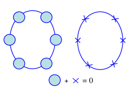
Figure 52: Mechanism of cancellation of reducible graphs. The ”X” denotes $J(\lambda)-J(\lambda=0)$ and the circles in blue are the self-energy insertions that make the graph reducible.

The role of the coupling constant integration is to provide the standard symmetry factors in the free energy graphs.

C.4 The total energy

In this subsection, we want to derive the relationship between the total energy of the system and the corresponding Green’s function. Let us start by the definition of the Green’s function

$$G(x_{1},x_{2})=-\langle T_{\tau}\psi(x_{1})\psi^{\dagger}(x_{2})\rangle.$$ (299)

The non–interacting (quadratic) part of the Hamiltonian

$$\beta H_{0}=\int dx_{1}dx_{2}\psi^{\dagger}(x_{1})H0_{x_{1}x_{2}}\delta(\tau_{1}-\tau_{2})\psi(x_{2}),$$ (300)

can be expressed by the Green’s function in the following way

$$\beta\langle H_{0}\rangle=\int dx_{1}dx_{2}H0_{x_{1}x_{2}}\delta(\tau_{1}-\tau_{2})\langle\psi^{\dagger}(x_{1})\psi(x_{2})\rangle$$ (301)

$$=\int dx_{1}dx_{2}H0_{x_{1}x_{2}}G(x_{2},x_{1})\delta(\tau_{2}-\tau_{1}+0^{+}).$$ (302)

To get the interacting part of the total energy, we are going to examine the time derivative of the Green’s function which follows directly from the definition Eq. (299) and takes the form

$$\left(\frac{\partial G(x_{1},x_{2})}{\partial\tau_{1}}\right)_{\begin{array}[]{l}\tau_{1}\rightarrow\tau_{2}-0^{+}\\ \mathbf{r}_{1}\rightarrow\mathbf{r}_{2}\end{array}}=\langle\psi^{\dagger}(x_{1})\left[H-\mu n,\psi(x_{1})\right]\rangle.\ \ \ \ \$$ (305)

The resulting commutator can be simplified by noting that the following two commutators take a very simple form

$$\int dx\psi^{\dagger}(x)\left[\psi(x),V\right] =2V$$ (306)

$$\int dx\psi^{\dagger}(x)\left[\psi(x),H_{0}\right] =H_{0}.$$ (307)

where $V$ is the normal–ordered electron–electron interaction. The factor two in the above equation follows from the fact that the interaction term is quartic in $\psi$ while $H_{0}$ is quadratic.

It is more convenient to express the equations in imaginary frequency than the imaginary time. Using the transformation

$$G(x_{1},x_{2})=T\sum_{i\omega}e^{-i\omega(\tau_{1}-\tau_{2})}G_{i\omega}(\mathbf{r}_{1},\mathbf{r}_{2}),$$ (308)

one obtains for the non–interacting part

$$T\int d\mathbf{r}_{1}d\mathbf{r}_{2}H0_{\mathbf{r}_{1}\mathbf{r}_{2}}\sum_{i\omega}G_{i\omega}(\mathbf{r}_{2},\mathbf{r}_{1})e^{i\omega 0^{+}}=\langle H_{0}\rangle,$$ (309)

while the time derivative from Eq. (305) gives

$$T\int d\mathbf{r}_{1}\sum_{i\omega}(i\omega)e^{i\omega 0^{+}}G_{i\omega}(\mathbf{r}_{1},\mathbf{r}_{1})=\langle H_{0}+2V-\mu n\rangle.$$ (310)

Combining equations (309) and (310) leads to the following expression for the interaction energy

$$\langle V\rangle=\frac{1}{2}T\int d\mathbf{r}_{1}d\mathbf{r}_{2}\sum_{i\omega}e^{i\omega 0+}\left[(i\omega+\mu)\delta(\mathbf{r}_{1}-\mathbf{r}_{2})-H0_{\mathbf{r}_{1}\mathbf{r}_{2}}\right]G_{i\omega}(\mathbf{r}_{2},\mathbf{r}_{1})=\frac{1}{2}\mbox{Tr}[e^{i\omega 0+}\;G_{0}^{-1}G]=\frac{1}{2}\mbox{Tr}[\Sigma G].$$ (311)

Here we took into account that $\sum_{i\omega}e^{i\omega 0+}=0$. Finally, the total energy becomes

$$\langle H\rangle=\frac{1}{2}T\int d\mathbf{r}_{1}d\mathbf{r}_{2}\sum_{i\omega}e^{i\omega 0+}\left[(i\omega+\mu)\delta(\mathbf{r}_{1}-\mathbf{r}_{2})+H0_{\mathbf{r}_{1}\mathbf{r}_{2}}\right]G_{i\omega}(\mathbf{r}_{2},\mathbf{r}_{1})=\mbox{Tr}[H_{0}G+\frac{1}{2}\Sigma G].$$ (312)

References

- Abrikosov (1965) Abrikosov, A. A., 1965, Physica 2, 21.
- Si et. al. et al. (1999) Si et. al., S., J. L. Smith, and K. Ingersent, 1999, Int. J. Mod. Phys. B 13, 2331.
- Al-Attar and Kakehashi (1999) Al-Attar, H., and Y. Kakehashi, 1999, J. Appl. Phys. 86, 3265.
- Allen and Liu (1992) Allen, J. W., and L. Z. Liu, 1992, Phys. Rev. B 46, 5047.
- Allen and Martin (1982) Allen, J. W., and R. M. Martin, 1982, Phys. Rev. Lett. 49, 1106.
- Almbladh et al. (1999) Almbladh, C. O., U. Von Barth, and R. Van Leeuwen, 1999, Int. J. Mod. Phys. B 13, 535.
- Altmann et al. (2000) Altmann, K. N., D. Y. Petrovykh, G. J. Mankey, N. Shannon, N. Gilman, M. Hochstrasser, R. F. Willis, and F. J. Himpsel, 2000, Phys. Rev. B 61, 15661.
- Amadon et al. (2005) Amadon, B., S. Biermann, and A. G. andF. Aryasetiawan, 2005, Electronic archive, xxx.lanl.gov, cond-mat/0504732 .
- Andersen (1975) Andersen, O. K., 1975, Phys. Rev. B 12, 3060.
- Andersen and Jepsen (1984) Andersen, O. K., and O. Jepsen, 1984, Phys. Rev. Lett. 53, 2571.
- Anderson (1961) Anderson, P. W., 1961, Phys. Rev. 124, 41.
- Anisimov et al. (1997a) Anisimov, V., A. Poteryaev, M. Korotin, A. Anokhin, and G. Kotliar, 1997a, J. Phys.: Condens. Matter 9, 7359.
- Anisimov et al. (1997b) Anisimov, V. I., F. Aryasetiawan, and A. I. Lichtenstein, 1997b, J. Phys.: Condens. Matter 9, 767.
- Anisimov and Gunnarsson (1991) Anisimov, V. I., and O. Gunnarsson, 1991, Phys. Rev. B 43, 7570.
- Anisimov et al. (2002) Anisimov, V. I., I. A. Nekrasov, D. E. Kondakov, T. M. Rice, and M. Sigrist, 2002, Eur. Phys. J. B 25, 191.
- Anisimov et al. (1991) Anisimov, V. I., J. Zaanen, and O. K. Andersen, 1991, Phys. Rev. B 44, 943.
- Antropov et al. (1996) Antropov, V. P., M. I. Katsnelson, B. N. Harmon, M. van Schilfgaarde, and D. Kusnezov, 1996, Phys. Rev. B 54, 1019.
- Argaman and Makov (2000) Argaman, N., and G. Makov, 2000, Am. J. Phys. 68, 69.
- Arita and Held (2005) Arita, R., and K. Held, 2005, Electronic archive, xxx.lanl.gov, cond-mat/0504040 .
- Arita et al. (2004) Arita, R., T. Miyake, T. Kotani, M. van Schilfgaarde, T. Oka, K. Kuroki, Y. Nozue, and H. Aoki, 2004, Phys. Rev. B 69, 195106.
- Arko et al. (2000) Arko, A. J., J. J. Joyce, L. Morales, J. Wills, J. Lashley, F. Wastin, and J. Rebizant, 2000, Phys. Rev. B 62, 1773.
- Arnaud and Alouani (2000) Arnaud, B., and M. Alouani, 2000, Phys. Rev. B 62, 4464.
- Aryanpour et al. (2002) Aryanpour, K., M. H. Hettler, and M. Jarrell, 2002, Phys. Rev. B 65, 153102.
- Aryanpour et al. (2005) Aryanpour, K., T. Maier, and M. Jarrell, 2005, Phys. Rev. B 71, 037101.
- Aryasetiawan et al. (2004a) Aryasetiawan, F., S. Biermann, and A. Georges, 2004a, Electronic archive, xxx.lanl.gov, cond-mat/0401626 .
- Aryasetiawan and Gunnarsson (1998) Aryasetiawan, F., and O. Gunnarsson, 1998, Rep. Prog. Phys. 61, 237.
- Aryasetiawan et al. (2004b) Aryasetiawan, F., M. Imada, A. Georges, G. Kotliar, S. Biermann, and A. I. Lichtenstein, 2004b, Phys. Rev. B 70, 195104.
- Bandyopadhyay and Sarma (1989) Bandyopadhyay, M. T., and D. D. Sarma, 1989, Phys. Rev. B 39, 3517.
- Barnes (1976) Barnes, S. E., 1976, J. Phys. F 6, 1375.
- Barnes (1977) Barnes, S. E., 1977, J. Phys. F 7, 2637.
- Baroni et al. (1987) Baroni, S., P. Gainnozzi, and A. Testa, 1987, Phys. Rev. Lett. 58, 1861.
- Baroni et al. (2001) Baroni, S., S. de Gironcoli, A. D. Corso, and P. Giannozzi, 2001, Rev. Mod. Phys. 73, 515.
- von Barth and Hedin (1972) von Barth, U., and L. Hedin, 1972, J. Phys. C 5, 1629.
- Baym (1962) Baym, G., 1962, Phys. Rev. 127, 1391.
- Baym and Kadanoff (1961) Baym, G., and L. P. Kadanoff, 1961, Phys. Rev. 124, 287.
- Belitz and Kirkpatrick (2002) Belitz, D., and T. R. Kirkpatrick, 2002, Phys. Rev. Lett. 89, 247202.
- Benedetti and Zeyher (1999) Benedetti, P., and R. Zeyher, 1999, Phys. Rev. B 59, 9923.
- Bickers and Scalapino (1989) Bickers, N. E., and D. J. Scalapino, 1989, Ann. Phys. (N.Y.) 193, 206.
- Bickers and White (1991) Bickers, N. E., and S. R. White, 1991, Phys. Rev. B 43, 8044.
- Biermann et al. (2003) Biermann, S., F. Aryasetiawan, and A. Georges, 2003, Phys. Rev. Lett. 90, 086402.
- Biermann et al. (2004) Biermann, S., F. Aryasetiawan, and A. Georges, 2004, Electronic archive, xxx.lanl.gov, cond-mat/0401653 .
- Biermann et al. (2005a) Biermann, S., L. de’ Medici, and A. Georges, 2005a, Electronic archive, xxx.lanl.gov, cond-mat/0505737 .
- Biermann et al. (2001) Biermann, S., A. Georges, A. Lichtenstein, and T. Giamarchi, 2001, Phys. Rev. Lett. 87, 276405.
- Biermann et al. (2005b) Biermann, S., A. Poteryaev, A. I. Lichtenstein, and A. Georges, 2005b, Phys. Rev. Lett. 94, 026404.
- Biroli and Kotliar (2002) Biroli, G., and G. Kotliar, 2002, Phys. Rev. B 65, 155112.
- Biroli and Kotliar (2004) Biroli, G., and G. Kotliar, 2004, Electronic archive, xxx.lanl.gov, cond-mat/0404537 .
- Biroli and Kotliar (2005) Biroli, G., and G. Kotliar, 2005, Phys. Rev. B 71, 037102.
- Biroli et al. (2004) Biroli, G., O. Parcollet, and G. Kotliar, 2004, Phys. Rev. B 69, 205108.
- Blankenbecler et al. (1981) Blankenbecler, R., D. J. Scalapino, and R. L. Sugar, 1981, Phys. Rev. D 24, 2278.
- Blawid et al. (2003) Blawid, S., A. Deppeler, and A. J. Millis, 2003, Phys. Rev. B 67, 165105.
- Blöechl (1989) Blöechl, P., 1989, Total Energies, Forces and Metal-Semiconductor Interfaces, Ph.D. thesis, Max-Planck Instuture für Festkoeperforschung, Stuttgart, Germany.
- Bohm and Pines (1951) Bohm, D., and D. Pines, 1951, Phys. Rev. 82, 625.
- Bohm and Pines (1952) Bohm, D., and D. Pines, 1952, Phys. Rev. 85, 338.
- Bohm and Pines (1953) Bohm, D., and D. Pines, 1953, Phys. Rev. 92, 609.
- Bolech et al. (2003) Bolech, C. J., S. S. Kancharla, and G. Kotliar, 2003, Phys. Rev. B 67, 75110.
- Bonca and Gubernatis (1993) Bonca, J., and J. E. Gubernatis, 1993, Phys. Rev. B 47, 13137.
- Boring and Smith (2000) Boring, A. M., and J. L. Smith, 2000, Los Alamos Science 26, 91.
- Bouchet et al. (2000) Bouchet, J., B. Siberchicot, F. Jollet, and A. Pasturel, 2000, J. Phys.: Condens. Matter 12, 1723.
- Bray and Moore (1980) Bray, A. J., and M. A. Moore, 1980, J. Phys. C 13(24), L655.
- Bronold and Fehske (2003) Bronold, F. X., and H. Fehske, 2003, Inst. Phys. Jagellonian Univ. Acta Physica Polonica B 34, 851.
- Bruno (2003) Bruno, P., 2003, Phys. Rev. Lett. 90, 087205.
- Bucher et al. (1994) Bucher, B., Z. Schlesinger, P. C. Canfield, and Z. Fisk, 1994, Phys. Rev. Lett. 72, 522.
- Bulut et al. (1993) Bulut, N., D. Scalapino, and S. White, 1993, Phys. Rev. B 47, 2742.
- Bünemann et al. (2003) Bünemann, J., F. Gebhard, T. Ohm, R. Umstätter, S. Weiser, W. Weber, R. Claessen, D. Ehm, A. Harasawa, A. Kakizak, A. Kimura, G. Nicolay, et al., 2003, Europhys. Lett. 61, 667.
- Bünemann and Weber (1997) Bünemann, J., and W. Weber, 1997, Phys. Rev. B 55, 4011.
- Bünemann et al. (1998) Bünemann, J., W. Weber, and F. Gebhard, 1998, Phys. Rev. B 57, 6896.
- C. Knecht and N. Blümer and P. G. J. van Dongen (2005) C. Knecht and N. Blümer and P. G. J. van Dongen, 2005, Electronic archive, xxx.lanl.gov, cond-mat/0505106 .
- Caffarel and Krauth (1994) Caffarel, M., and W. Krauth, 1994, Phys. Rev. Lett. 72, 1545.
- Capellmann (1974) Capellmann, H., 1974, J. Phys. F: Met. Phys. 4, 1466.
- Capone et al. (2004) Capone, M., M. Civelli, S. S. Kancharla, C. Castellani, and G. Kotliar, 2004, Phys. Rev. B 69, 195105.
- Capone et al. (2002a) Capone, M., M. Fabrizio, C. Castellani, and E. Tosatti, 2002a, Science 296, 2364.
- Capone et al. (2000) Capone, M., M. Fabrizio, P. Giannozzi, and E. Tosatti, 2000, Phys. Rev. B 62, 7619.
- Capone et al. (2002b) Capone, M., M. Fabrizio, and E. Tosatti, 2002b, J. Phys. Chem. Solids 63, 1555.
- Castellani et al. (1979) Castellani, C., C. Di Castro, D. Feinberg, and J. Ranninger, 1979, Phys. Rev. Lett. 43, 1957.
- Castellani et al. (1992) Castellani, C., G. Kotliar, R. Raimondi, M. Grilli, Z. Wang, and M. Rozenberg, 1992, Phys. Rev. Lett. 69, 2009.
- Castellani et al. (1978a) Castellani, C., C. R. Natoli, and J. Ranninger, 1978a, Phys. Rev. B 18, 4945.
- Castellani et al. (1978b) Castellani, C., C. R. Natoli, and J. Ranninger, 1978b, Phys. Rev. B 18, 5001.
- Ceperley and Alder (1980) Ceperley, D. M., and B. J. Alder, 1980, Phys. Rev. Lett. 45, 566.
- Chattopadhyay et al. (2001) Chattopadhyay, A., S. Das Sarma, and A. J. Millis, 2001, Phys. Rev. Lett. 87, 227202.
- Chernyshev and Fishman (2003) Chernyshev, A. L., and R. S. Fishman, 2003, Phys. Rev. Lett. 90, 177202.
- Chioncel et al. (2003a) Chioncel, L., M. I. Katsnelson, R. A. de Groot, and A. I. Lichtenstein, 2003a, Phys. Rev. B 68, 144425.
- Chioncel et al. (2005) Chioncel, L., M. I. Katsnelson, G. A. de Wijs, R. A. de Groot, and A. I. Lichtenstein, 2005, Phys. Rev. B 71, 85111.
- Chioncel and Lichtenstein (2004) Chioncel, L., and A. I. Lichtenstein, 2004, Electronic archive, xxx.lanl.gov, cond-mat/0403685 .
- Chioncel et al. (2003b) Chioncel, L., L. Vitos, I. A. Abrikosov, J. Kollar, M. I. Katsnelson, and A. I. Lichtenstein, 2003b, Phys. Rev. B 67, 235106.
- Chioncel et al. (2003c) Chioncel, L., L. Vitos, I. A. Abrikosov, J. Kollar, M. I. Katsnelson, and A. I. Lichtenstein, 2003c, Phys. Rev. B 67, 235106.
- Chitra and Kotliar (1999) Chitra, R., and G. Kotliar, 1999, Phys. Rev. Lett. 83, 2386.
- Chitra and Kotliar (2000a) Chitra, R., and G. Kotliar, 2000a, Phys. Rev. B 62, 12715.
- Chitra and Kotliar (2000b) Chitra, R., and G. Kotliar, 2000b, Phys. Rev. Lett. 84, 3678.
- Chitra and Kotliar (2001) Chitra, R., and G. Kotliar, 2001, Phys. Rev. B 63, 115110.
- Ciuchi and De Pasquale (1999) Ciuchi, S., and F. De Pasquale, 1999, Phys. Rev. B 59, 5431.
- Ciuchi et al. (1997) Ciuchi, S., F. de Pasquale, S. Fratini, and D. Feinberg, 1997, Phys. Rev. B 56, 4494.
- Civelli et al. (2005) Civelli, M., M. Capone, S. S. Kancharla, O. Parcollet, and G. Kotliar, 2005, Phys. Rev. Lett. 95, 106402.
- Coleman (1984) Coleman, P., 1984, Phys. Rev. B 29, 3035.
- Cornwall et al. (1974) Cornwall, J. M., R. Jackiw, and E. Tomboulis, 1974, Phys. Rev. D 10, 2428.
- Costi (1986) Costi, T. A., 1986, J. Phys. C 19, 5665.
- Costi et al. (1996) Costi, T. A., J. Kroha, and P. Wölfle, 1996, Phys. Rev. B 53, 1850.
- Cox and Ruckenstein (1993) Cox, D. L., and A. E. Ruckenstein, 1993, Phys. Rev. Lett. 71, 1613.
- Craco et al. (2003a) Craco, L., M. Laad, and E. Müller-Hartmann, 2003a, Phys. Rev. B 68, 233310.
- Craco et al. (2003b) Craco, L., M. Laad, and E. Müller-Hartmann, 2003b, Phys. Rev. Lett. 90, 237203.
- Crandles et al. (1992) Crandles, D. A., T. Timusk, J. D. Garrett, and J. E. Greedan, 1992, Physica C 201, 407.
- Cyrot (1970) Cyrot, M., 1970, Phys. Rev. Lett. 25, 871.
- Dagotto (1994) Dagotto, E., 1994, Rev. Mod. Phys. 66, 763.
- Dagotto (2002) Dagotto, E., 2002, Nanoscale Phase Separation and Colossal Magnetoresistance : The Physics of Manganites and Related Compounds (Springer-Verlag, Berlin, Germany).
- Dahnken et al. (2004) Dahnken, C., M. Aichhorn, W. Hanke, E. Arrigoni, and M. Potthoff, 2004, Physical Review B-Condensed Matter 70, 245110.
- Dahnken et al. (2002) Dahnken, C., E. Arrigoni, and W. Hanke, 2002, J. Low Temp. Phys. 126, 949.
- Dahnken et al. (2005) Dahnken, C., M. Potthoff, E. Arrigoni, and W. Hanke, 2005, Electronic archive, xxx.lanl.gov, cond-mat/0504618 .
- Dai et al. (2005) Dai, X., K. Haule, and G. Kotliar, 2005, Phys. Rev. B 72, 045111.
- Dai et al. (2003) Dai, X., S. Y. Savrasov, G. Kotliar, A. Migliori, H. Ledbetter, and E. Abrahams, 2003, Science 300, 953.
-
Damascelli (1999)
Damascelli, A.,
1999,
http://www.ub.rug.nl/eldoc/dis/science/a.damascelli/ . - Das Sarma et al. (2003) Das Sarma, S., E. H. Hwang, and A. Kaminski, 2003, Phys. Rev. B 67, 155201.
- de’ Medici et al. (2005a) de’ Medici, L., A. Georges, and S. Biermann, 2005a, Electronic archive, xxx.lanl.gov, cond-mat/0503764 .
- de’ Medici et al. (2005b) de’ Medici, L., A. Georges, G. Kotliar, and S. Biermann, 2005b, Electronic archive, xxx.lanl.gov, cond-mat/0502563 .
- Dederichs et al. (1984) Dederichs, P. H., S. Blugel, R. Zeller, and H. Akai, 1984, Phys. Rev. Lett. 53, 2512.
- deDominicis and Martin (1964a) deDominicis, C., and P. Martin, 1964a, J. Math. Phys. 5, 14.
- deDominicis and Martin (1964b) deDominicis, C., and P. Martin, 1964b, J. Math. Phys. 5, 31.
- Deppeler and Millis (2002a) Deppeler, A., and A. J. Millis, 2002a, Phys. Rev. B 65, 224301.
- Deppeler and Millis (2002b) Deppeler, A., and A. J. Millis, 2002b, Phys. Rev. B 65, 100301.
- Desclaux and Freeman (1984) Desclaux, J. P., and A. J. Freeman, 1984, in Handbook on the Physics and Chemistry of the Actinides, edited by A. J. Freeman and G. H. Lander (Elsevier, Amsterdam), volume 1, p. 46.
- Dobrosavljec et al. (2003) Dobrosavljec, V., A. A. Pastor, and B. K. Nikolic, 2003, Europhys. Lett. 62, 76.
- Dobrosavljevic and Kotliar (1997) Dobrosavljevic, V., and G. Kotliar, 1997, Phys. Rev. Lett. 78, 3943.
- Dobson et al. (1997) Dobson, J. F., G. Vignale, and M. P. Das (eds.), 1997, Electronic Density Functional Theory: Recent Progress and New Directions (Plenum, New York).
- Drchal et al. (1999) Drchal, V., V. Janiš, and J. Kudrnovský, 1999, Phys. Rev. B 60, 15664.
- Drchal et al. (2005) Drchal, V., V. Janiš, J. Kudrnovsky, V. S. Oudovenko, X. Dai, K. Haule, and G. Kotliar, 2005, J. Phys.: Condens. Matter 17, 61.
- Eberhardt and Plummer (1980) Eberhardt, W., and E. W. Plummer, 1980, Phys. Rev. B 21, 3245.
- Edwards and Rao (1990) Edwards, P., and C. N. Rao (eds.), 1990, Metal-Insulator Transitions Revisited (Taylor & Francis, London).
- Eldridge et al. (1991) Eldridge, J. E., K. Kornelsen, H. H. Wang, J. M. Williams, A. V. S. Crouch, and D. M. Watkins, 1991, Solid State Commun. 79, 583.
- Eliashberg and Capellmann (1998) Eliashberg, G., and H. Capellmann, 1998, JETP Lett. 67, 111.
- Eriksson et al. (1999) Eriksson, O., J. D. Becker, A. V. Balatsky, and J. M. Wills, 1999, J. Alloys Compd. 287, 1.
- Evenson et al. (1970) Evenson, W. E., S. Q. Wang, and J. R. Schrieffer, 1970, Phys. Rev. B 2, 2604.
- Ezhov et al. (1999) Ezhov, S. Y., V. I. Anisimov, D. I. Khomskii, and G. A. Sawatzky, 1999, Phys. Rev. Lett. 83, 4136.
- Faulkner (1982) Faulkner, J., 1982, Prog. Mater. Sci. 1, 27.
- Feldbacher et al. (2004) Feldbacher, M., K. Held, and F. F. Assaad, 2004, Phys. Rev. Lett. 93, 136405.
- Ferrer et al. (1987) Ferrer, J., A. Martín-Rodero, and F. Flores, 1987, Phys. Rev. B 36, 6149.
- Ferrero et al. (2005) Ferrero, M., F. Becca, M. Fabrizio, and M. Capone, 2005, Electronic archive, xxx.lanl.gov, cond-mat/0503759 .
- Fetter and Walecka (1971) Fetter, A., and J. Walecka, 1971, Quantum Theory of Many-Particle Systems (McGraw-Hill, New York).
- Fishman and Jarrell (2002) Fishman, R. S., and M. Jarrell, 2002, J. Appl. Phys. 91, 8120.
- Fishman and Jarrell (2003a) Fishman, R. S., and M. Jarrell, 2003a, J. Appl. Phys. 93, 7148.
- Fishman and Jarrell (2003b) Fishman, R. S., and M. Jarrell, 2003b, Phys. Rev. B 67, 100403.
- Florens and Georges (2002) Florens, S., and A. Georges, 2002, Phys. Rev. B 66, 165111.
- Florens and Georges (2004) Florens, S., and A. Georges, 2004, Phys. Rev. B 70(3), 35114.
- Florens et al. (2002) Florens, S., A. Georges, G. Kotliar, and O. Parcollet, 2002, Phys. Rev. B 66, 205102.
- Foulkes (1989) Foulkes, W. M. C., 1989, Unknown, Ph.D. thesis, Cambridge University.
- Fratini et al. (2000) Fratini, S., F. De Pasquale, and S. Ciuchi, 2000, Int. J. Mod. Phys. B 14, 3020.
- Fratini et al. (2001) Fratini, S., F. de Pasquale, and S. Ciuchi, 2001, Phys. Rev. B 63, 153101.
- Freeman and Darby (1974) Freeman, A. J., and J. B. Darby, 1974, The Actinides: Electronic Structure and Related Properties Vols 1 and 2 (Academic, New York).
- Freeman et al. (1987) Freeman, A. J., B. I. Min, and M. R. Norman, 1987, in Handbook on the Physics of Rare-Earths, edited by K. A. Gschneider, J. L. Eyring, and S. Hüfner (Elsevier, North-Holland, New York), volume 10, pp. 165–229.
- Freericks (2004) Freericks, J. K., 2004, Electronic archive, xxx.lanl.gov, cond-mat/0408226 .
- Freericks et al. (1993) Freericks, J. K., M. Jarrell, and D. J. Scalapino, 1993, Phys. Rev. B 48, 6302.
- Freericks and Zlatic (2003) Freericks, J. K., and V. Zlatic, 2003, Rev. Mod. Phys. 75, 1333.
- Fujimori et al. (1992a) Fujimori, A., I. Hase, M. Nakamura, H. Namatame, Y. Fujishima, Y. Tokura, M. Abbate, F. M. F. de Groot, M. T. Czyzyk, J. C. Fuggle, O. Strebel, F. Lopez, et al., 1992a, Phys. Rev. B 46, 9841.
- Fujimori et al. (1992b) Fujimori, A., I. Hase, H. Namatame, Y. Fujishima, Y. Tokura, H. Eisaki, S. Uchida, K. Takegahara, and F. M. F. de Groot, 1992b, Phys. Rev. Lett. 69, 1796.
- Fujishima et al. (1992) Fujishima, Y., Y. Tokura, T. Arima, and S. Uchida, 1992, Phys. Rev. B 46, 11167.
- Fukuda (1988) Fukuda, R., 1988, Phys. Rev. Lett. 61, 1549.
- Fukuda et al. (1995) Fukuda, R., M. Komachiya, S. Yokojima, Y. Suzuki, K. Okumura, and T. Inagaki, 1995, Prog. Theor. Phys. Suppl. 121, 1.
- Fukuda et al. (1994) Fukuda, R., T. Kotani, Y. Suzuki, and S. Yokojima, 1994, Prog. Theor. Phys. 92, 833.
- Furukawa (1994) Furukawa, N., 1994, J. Phys. Soc. Japan 63, 3214.
- Furukawa et al. (1999) Furukawa, Y., I. Okamura, K. Kumagai, T. Goto, T. Fukase, Y. Taguchi, and Y. Tokura, 1999, Phys. Rev. B 59, 10550.
- Furukawa et al. (1997) Furukawa, Y., I. Okamura, K. Kumagai, Y. Taguchi, and Y. Tokura, 1997, Physica B 237-238, 39.
- Fye and Hirsch (1989) Fye, R. M., and J. E. Hirsch, 1989, Phys. Rev. B 40, 4780 4796.
- Galitskii (1958) Galitskii, V. M., 1958, Soviet Phys. JETP 34, 698.
- Georges (1992) Georges, A., 1992, Phys. Rev. B 45, 6479.
- Georges (2002) Georges, A., 2002, in Strongly Correlated Fermions and Bosons in Low-Dimensional Disordered Systems, edited by I. V. Lerner, B. L. Althsuler, V. I. Fal’ko, and T. Giamarchi (Kluwer Academic Publishers, Dordrecht, Netherlands), NATO Science Series II.
- Georges (2004a) Georges, A., 2004a, AIP Conf. Proc. , 3.
- Georges (2004b) Georges, A., 2004b, Electronic archive, xxx.lanl.gov, cond-mat/0403123 .
- Georges et al. (2000) Georges, A., T. Giamarchi, and N. Sandler, 2000, Phys. Rev. B 61, 16393.
- Georges and Kotliar (1992) Georges, A., and G. Kotliar, 1992, Phys. Rev. B 45, 6479.
- Georges et al. (1993) Georges, A., G. Kotliar, and W. Krauth, 1993, Z. Phys. B 92, 313.
- Georges et al. (1996) Georges, A., G. Kotliar, W. Krauth, and M. J. Rozenberg, 1996, Rev. Mod. Phys. 68, 13.
- Georges and Krauth (1992) Georges, A., and W. Krauth, 1992, Phys. Rev. Lett. 69, 1240.
- Georges and Krauth (1993) Georges, A., and W. Krauth, 1993, Phys. Rev. B 48, 7167.
- Georges and Yedidia (1991a) Georges, A., and J. S. Yedidia, 1991a, J. Phys. A 24, 2173.
- Georges and Yedidia (1991b) Georges, A., and J. S. Yedidia, 1991b, Phys. Rev. B 43, 3475.
- Giamarchi et al. (2004) Giamarchi, T., S. Biermann, A. Georges, and A. Lichtenstein, 2004, J. de Physique 114, 23.
- Glazek and Wilson (1993) Glazek, S. D., and K. G. Wilson, 1993, Phys. Rev. D 48, 5863.
- Glazek and Wilson (1994) Glazek, S. D., and K. G. Wilson, 1994, Phys. Rev. D 49, 4214.
- Golub and Loan (1996) Golub, G., and C. V. Loan, 1996, Matrix Computations (MD: Johns Hopkins, Baltimore).
- Gonze et al. (1992) Gonze, X., D. C. Allan, and M. P. Teter, 1992, Phys. Rev. Lett. 68, 3603.
- Goodenough (1963) Goodenough, J., 1963, Magnetism and the Chemical Bond (John Wiley and Sons, New York).
- Goodenough (1971) Goodenough, J. B., 1971, Prog. Solid State Chem. 5, 145.
- Grempel and Rozenberg (1998) Grempel, D. R., and M. J. Rozenberg, 1998, Phys. Rev. Lett. 80, 389.
- Grempel and Si (2003) Grempel, D. R., and Q. Si, 2003, Phys. Rev. Lett. 91, 026401.
- Gros and Valenti (1993) Gros, C., and R. Valenti, 1993, Phys. Rev. B 48, 418.
- Gross et al. (1996) Gross, E. K. U., J. F. Dobson, and M. Petersilka, 1996, Density Functional Theory, Springer Series Topics in Current Chemistry (Springer, Heidelberg).
- Gunnarsson (1990) Gunnarsson, O., 1990, Phys. Rev. B 41, 514.
- Gunnarsson (1997) Gunnarsson, O., 1997, Rev. Mod. Phys. 69, 575.
- Gunnarsson et al. (1976) Gunnarsson, O., M. Jonson, and B. I. Lundqvist, 1976, Phys. Rev. A 59, 177.
- Gunnarsson and Koch (1997) Gunnarsson, O., and E. Koch, 1997, Phys. Lett. A 235, 530.
- Gunnarsson and Lundqvist (1976) Gunnarsson, O., and B. I. Lundqvist, 1976, Phys. Rev. B 13, 4274.
- Gyorffy et al. (1985) Gyorffy, B. L., A. J. Pindor, J. Staunton, G. M. Stocks, and H. Winter, 1985, J. Phys. F: Met. Phys. 15, 1337.
- Gyorffy and Stocks (1979) Gyorffy, B. L., and G. M. Stocks, 1979, in Electrons in Disordered Metals and at Metallic Surfaces, edited by P. Phariseau, B. L. Gyorffy, and L. Scheire (Plenum, New York), NATO ASI Series B42, pp. 89–192.
- Halilov et al. (1998) Halilov, S. V., H. Eschrig, A. Y. Perlov, and P. M. Oppeneer, 1998, Phys. Rev. B 58, 293.
- Han et al. (2003) Han, J. E., O. Gunnarsson, and V. H. Crespi, 2003, Phys. Rev. Lett. 90, 167006.
- Harris (1985) Harris, J., 1985, Phys. Rev. B 31, 1770.
- Harris and Jones (1974) Harris, J., and R. O. Jones, 1974, J. Phys. F: Met. Phys. 4, 1170.
- Hassan et al. (2004) Hassan, S., A. Georges, and H. Krishnamurthy, 2004, Electronic archive, xxx.lanl.gov, cond-mat/0405359 .
- Haule et al. (2001) Haule, K., S. Kirchner, J. Kroha, and P. Wölfle, 2001, Phys. Rev. B 64, 155111.
- Haule et al. (2005) Haule, K., V. Oudovenko, S. Y. Savrasov, and G. Kotliar, 2005, Phys. Rev. Lett. 94, 036401.
- Hays et al. (1999) Hays, C. C., J. S. Zhou, J. T. Markert, and J. B. Goodenough, 1999, Phys. Rev. B 60, 10367.
- Hecker and Timofeeva (2000) Hecker, S. S., and L. F. Timofeeva, 2000, Los Alamos Science 26, 244.
- Hedin (1965) Hedin, L., 1965, Phys. Rev. 139, A796.
- Hedin and Lundquist (1969) Hedin, L., and S. Lundquist, 1969, in Solid State Physics, edited by H. Ehrenreich, F. Seitz, and D. Turnbull (Academic, New York), volume 23, p. 1.
- Heid and Bohnen (1999) Heid, R., and K. P. Bohnen, 1999, Phys. Rev. B 60, R3709.
- Held et al. (2005) Held, K., J. W. Allen, V. I. Anisimov, V. Eyert, G. Keller, H.-D. Kim, and S.-K. M. andD. Vollhardt, 2005, Physica B 359-361, 642.
- Held et al. (2001a) Held, K., G. Keller, V. Eyert, D. Vollhardt, and V. I. Anisimov, 2001a, Phys. Rev. Lett. 86, 5345.
- Held et al. (2001b) Held, K., A. K. McMahan, and R. T. Scalettar, 2001b, Phys. Rev. Lett. 87, 276404.
- Held et al. (2001c) Held, K., I. A. Nekrasov, N. Blumer, V. I. Anisimov, and D. Vollhardt, 2001c, Int. J. Mod. Phys. B 15, 2611.
- Held et al. (2003) Held, K., I. A. Nekrasov, G. Keller, V. Eyert, N. Blümer, A. K. McMahan, R. T. Scalettar, T. Pruschke, V. I. Anisimov, and D. Vollhardt, 2003, Psi-k Newsletter #56, 65.
- Held and Vollhardt (1998) Held, K., and D. Vollhardt, 1998, Eur. Phys. J. B 5, 473.
- Held and Vollhardt (2000) Held, K., and D. Vollhardt, 2000, Phys. Rev. Lett. 84, 5168.
- Herring (1966) Herring, C., 1966, in Magnetism, edited by G. T. Rado and H. Suhl (Academic Press, New York, London), volume IV, pp. 345–385.
- Hesper et al. (2000) Hesper, R., L. H. Tjeng, A. Heeres, and G. A. Sawatzky, 2000, Phys. Rev. B 62, 16046.
- Hess and Serene (1999) Hess, D. W., and J. W. Serene, 1999, Phys. Rev. B 59, 15617.
- Hettler et al. (2000) Hettler, M. H., M. Mukherjee, M. Jarrell, and H. R. Krishnamurthy, 2000, Phys. Rev. B 61, 12739.
- Hettler et al. (1998) Hettler, M. H., A. N. Tahvildar-Zadeh, M. Jarrell, T. Pruschke, and H. R. Krishnamurthy, 1998, Phys. Rev. B 58, R7475.
- Hirsch (1983) Hirsch, J. E., 1983, Phys. Rev. B 28, 4059.
- Hirsch and Fye (1986) Hirsch, J. E., and R. M. Fye, 1986, Phys. Rev. Lett. 56, 2521.
- Hoinkis et al. (2005) Hoinkis, M., M. Sing, J. Schafer, M. Klemm, S. Horn, H. Benthien, E. Jeckelmann, T. Saha-Dasgupta, L. Pisani, R. Valenti, and R. Claessen, 2005, Phys. Rev. B 72, 125127.
- Holm (1999) Holm, B., 1999, Phys. Rev. Lett. 83, 788.
- Holm and von Barth (1998) Holm, B., and U. von Barth, 1998, Phys. Rev. B 57, 2108.
- Hubbard (1963) Hubbard, J., 1963, Proc. Roy. Soc. London A 276, 238.
- Hubbard (1979a) Hubbard, J., 1979a, Phys. Rev. B 19, 2626.
- Hubbard (1979b) Hubbard, J., 1979b, Phys. Rev. B 20, 4584.
- Hubbard (1981) Hubbard, J., 1981, Phys. Rev. B 23, 5974.
- Huscroft et al. (2001) Huscroft, C., M. Jarrell, T. Maier, S. Moukouri, , and A. N. Tahvildarzadeh, 2001, Phys. Rev. Lett. 86, 139.
- Hybertsen and Louie (1985) Hybertsen, M. S., and S. G. Louie, 1985, Phys. Rev. Lett. 55, 1418.
- Hybertsen and Louie (1986) Hybertsen, M. S., and S. G. Louie, 1986, Phys. Rev. B 34, 5390.
- Hybertsen et al. (1989) Hybertsen, M. S., M. Schlütter, and N. E. Christensen, 1989, Phys. Rev. B 39, 9028.
- Imada et al. (1998) Imada, M., A. Fujimori, and Y. Tokura, 1998, Rev. Mod. Phys. 70, 1039.
- Imai and Kawakami (2000) Imai, Y., and N. Kawakami, 2000, J. Phys. Soc. Japan 69, 3063.
- Imseok et al. (2001) Imseok, Y., S. Y. Savrasov, and G. Kotliar, 2001, Phys. Rev. Lett. 87, 216405.
- Ingersent and Si (2002) Ingersent, K., and Q. Si, 2002, Phys. Rev. Lett. 89, 076403.
- Inoue et al. (2002) Inoue, I., C. Bergemann, I. Hase, and S. R. Julian, 2002, Phys. Rev. Lett. 88, 236403.
- Irkhin et al. (2004) Irkhin, V., M. Katsnelson, and A. Lichtenstein, 2004, Electronic archive, xxx.lanl.gov, cond-mat/0406487 .
- Irkhin and Katsnelson (1994) Irkhin, V. Y., and M. I. Katsnelson, 1994, Physics - Uspekhi 37, 659.
- Ishida et al. (2005) Ishida, H., M. D. Johannes, and A. Liebsch, 2005, Phys. Rev. Lett. 94, 196401.
- Ito et al. (1996) Ito, H., T. Ishiguro, M. Kubota, and G. Saito, 1996, J. Phys. Soc. Japan 65, 2987.
- IV et al. (1992) IV, J. E. S., S. M. Kauzlarich, and P. Klavins, 1992, Chem. Mater. 4, 346.
- Iwan et al. (1979) Iwan, M., F. J. Himpsel, and D. E. Eastman, 1979, Phys. Rev. Lett. 43, 1829.
- Izyumov Yu and Letfulov (2001) Izyumov Yu, A., and B. M. Letfulov, 2001, Trans Tech Publications. Materials Science Forum 373-376, 681.
- J. T. Devreese and Camp (1983) J. T. Devreese, V. E. V. D., and P. E. V. Camp (eds.), 1983, Ab inition Calculations of Phonon Spectra (Plenum Press, New York).
- Jarrell (1992) Jarrell, M., 1992, Phys. Rev. Lett. 69, 168.
- Jarrell and Akhlaghpour (1993) Jarrell, M., and T. Akhlaghpour, H. Pruschke, 1993, in Quantum Monte Carlo Methods in Condensed Matter Physics, edited by M. Suzuki (World Scientific, Singapore), pp. 221–234.
- Jarrell and Gubernatis (1996) Jarrell, M., and J. E. Gubernatis, 1996, Phys. Rep. 269, 133.
- Jeschke and Kotliar (2005) Jeschke, H. O., and G. Kotliar, 2005, Phys. Rev. B 71(8), 85103.
- Jian-Xin et al. (2003) Jian-Xin, Z., D. R. Grempel, and Q. Si, 2003, Phys. Rev. Lett. 91, 156404.
- Johansson (1974) Johansson, B., 1974, Phil. Mag. 30, 469.
- Johansson et al. (1995) Johansson, B., I. A. Abrikosov, M. Aldén, A. V. Ruban, and H. L. Skriver, 1995, Phys. Rev. Lett. 74, 2335.
- Jones et al. (2000) Jones, M. D., J. C. Boettger, R. C. Albers, and D. J. Singh, 2000, Phys. Rev. B 61, 4644.
- Kagawa et al. (2003) Kagawa, F., T. Itou, K. Miyagawa, and K. Kanoda, 2003, Phys. Rev. B , 064511.
- Kagawa et al. (2004) Kagawa, F., T. Itou, K. Miyagawa, and K. Kanoda, 2004, Phys. Rev. Lett. 93, 127001/1.
- Kajueter (1996a) Kajueter, H., 1996a, Interpolating perturbation scheme for correlated electron systems, Ph.D. thesis, Rutgers University, Graduate School New Brunswick, NJ.
- Kajueter (1996b) Kajueter, H., 1996b, Interpolating perturbation scheme for correlated electron systems, Ph.D. thesis, Rutgers University.
- Kajueter and Kotliar (1996a) Kajueter, H., and G. Kotliar, 1996a, unpublished.
- Kajueter and Kotliar (1996b) Kajueter, H., and G. Kotliar, 1996b, Phys. Rev. Lett. 77, 131.
- Kajueter and Kotliar (1997) Kajueter, H., and G. Kotliar, 1997, Int. J. Mod. Phys. B 11, 729.
- Kajueter et al. (1997) Kajueter, H., G. Kotliar, D. D. Sarma, and S. Barman, 1997, Int. J. Mod. Phys. B 11, 3849.
- Kakehashi (1992) Kakehashi, Y., 1992, Phys. Rev. B 45, 7196.
- Kakehashi (2002) Kakehashi, Y., 2002, Phys. Rev. B 65, 184420.
- Kakehashi et al. (1998) Kakehashi, Y., S. Akbar, and N. Kimura, 1998, Phys. Rev. B 57, 8354.
- Kakizaki et al. (1994) Kakizaki, A., J. Fujii, K. Shimada, A. Kamata, K. Ono, K. Park, T. Kinoshita, T. Ishii, and H. Fukutani, 1994, Phys. Rev. Lett. 72, 2781.
- Kanamori (1963) Kanamori, J., 1963, Prog. Theor. Phys. 30, 275.
- Kanoda (2004) Kanoda, K., 2004, private communication.
- Katsnelson and Lichtenstein (2000) Katsnelson, M. I., and A. I. Lichtenstein, 2000, Phys. Rev. B 61, 8906.
- Katsnelson and Lichtenstein (2002) Katsnelson, M. I., and A. I. Lichtenstein, 2002, Eur. Phys. J. B 30, 9.
- Keller et al. (2005) Keller, G., K. H. andV. Eyert, D. Vollhardt, and V. I. Anisimov, 2005, Phys. Rev. B 70, 205116.
- Kikugawa et al. (2004) Kikugawa, N., A. Mackenzie, C. Bergemann, and Y. Maeno, 2004, Phys. Rev. B 70, 174501.
- Kino and Fukuyama (1996) Kino, H., and H. Fukuyama, 1996, J. Phys. Soc. Japan 65, 2158.
- Kisker et al. (1984) Kisker, E., K. Schröder, M. Campagna, and W. Gudat, 1984, Phys. Rev. Lett. 52, 2285.
- Kobayashi et al. (1996) Kobayashi, Y., S. Taniguchi, M. Kasai, M. Sato, T. Nishioka, and M. Kontani, 1996, J. Phys. Soc. Japan 65, 3978.
- Koelling and Harmon (1977) Koelling, D., and B. Harmon, 1977, JPC 10, 3107.
- Koga et al. (2005) Koga, A., N. Kawakami, T. Rice, and M. Sigrist, 2005, Electronic archive, xxx.lanl.gov, cond-mat/0503651 .
- Koga et al. (2004) Koga, A., N. Kawakami, T. M. Rice, and M. Sigrist, 2004, Phys. Rev. Lett. 92, 216402.
- Korenman et al. (1977a) Korenman, V., J. L. Murray, and R. E. Prange, 1977a, Phys. Rev. B 16, 4032.
- Korenman et al. (1977b) Korenman, V., J. L. Murray, and R. E. Prange, 1977b, Phys. Rev. B 16, 4048.
- Korenman et al. (1977c) Korenman, V., J. L. Murray, and R. E. Prange, 1977c, Phys. Rev. B 16, 4058.
- Kotani (2000) Kotani, T., 2000, J. Phys.: Condens. Matter 12, 2413.
- Kotliar (1999a) Kotliar, G., 1999a, Eur. Phys. J. B 11, 27.
- Kotliar (1999b) Kotliar, G., 1999b, Physica B 261, 711.
- Kotliar (2001) Kotliar, G., 2001, in Open Problems in Strongly Correlated Electron Systems, edited by J. Bonca, S. Sarkar, P. Prelovsek, and A. Ramsak (Kluwer Academic Publishers, Netherlands), NATO Science Series II, pp. 325–336.
- Kotliar (2003) Kotliar, G., 2003, Science 302, 67.
- Kotliar (2005) Kotliar, G., 2005, J. Phys. Soc. Japan 74, 147.
- Kotliar and Kajueter (1996) Kotliar, G., and H. Kajueter, 1996, Phys. Rev. B 54, R14221.
- Kotliar et al. (2000) Kotliar, G., E. Lange, and M. J. Rozenberg, 2000, Phys. Rev. Lett. 84, 5180.
- Kotliar et al. (2002) Kotliar, G., S. Murthy, and M. J. Rozenberg, 2002, Phys. Rev. Lett. 89, 046401.
- Kotliar and Ruckenstein (1986) Kotliar, G., and A. E. Ruckenstein, 1986, Phys. Rev. Lett. 57, 1362.
- Kotliar and Savrasov (2001) Kotliar, G., and S. Savrasov, 2001, in New Theoretical approaches to strongly correlated systems, edited by A. M. Tsvelik (Kluwer Academic Publishers, The Netherlands), pp. 259–301.
- Kotliar et al. (2001) Kotliar, G., S. Y. Savrasov, G. Palsson, and G. Biroli, 2001, Phys. Rev. Lett. 87, 186401.
- Kotliar and Vollhardt (2004) Kotliar, G., and D. Vollhardt, 2004, Physics Today 57, 53.
- Kreutz et al. (1989) Kreutz, T. J., T. Greber, P. Aebi, and J. Osterwalder, 1989, Phys. Rev. B 58, 1300.
- Kroha et al. (1997) Kroha, J., P. Wölfle, and T. A. Costi, 1997, Phys. Rev. Lett. 79, 261.
- Kübler (2000) Kübler, J., 2000, Theory of Itinerant Electron Magnetism (Oxford University Press).
- Kuebler (2002) Kuebler, J., 2002, Adv. Solid State Phys. 42, 407.
- Kumagai et al. (1993) Kumagai, K., T. Suzuki, Y. Taguchi, Y. Okada, Y. Fujishima, and Y. Tokura, 1993, Phys. Rev. B 48, 7636.
- Kutepov and Kutepova (2003) Kutepov, A., and S. Kutepova, 2003, JPCM 15, 2607.
- Kuwamoto et al. (1980) Kuwamoto, H., J. M. Honig, and J. Appel, 1980, Phys. Rev. B 22, 2626.
- Laad et al. (2001) Laad, M., L. Craco, and E. Müller-Hartmann, 2001, Phys. Rev. B 64, 214421.
- Laad et al. (2003a) Laad, M., L. Craco, and E. Müller-Hartmann, 2003a, Phys. Rev. B 67, 033105.
- Laad et al. (2003b) Laad, M., L. Craco, and E. Müller-Hartmann, 2003b, Phys. Rev. Lett. 91, 156402.
- Lambin and Vigneron (1984) Lambin, P., and J. P. Vigneron, 1984, Phys. Rev. B 29, 3430.
- Lange and Kotliar (1999) Lange, E., and G. Kotliar, 1999, Phys. Rev. B 59, 1800.
- Langreth and Perdew (1977) Langreth, D. C., and J. P. Perdew, 1977, Phys. Rev. B 15, 2884.
- Lashley et al. (2004) Lashley, J. C., A. C. Lawson, R. J. McQueeney, and G. H. Lander, 2004, Electronic archive, xxx.lanl.gov, cond-mat/0410634 .
- Lavagna (1990) Lavagna, M., 1990, Phys. Rev. B 41, 142.
- Lechermann et al. (2005a) Lechermann, F., S. Biermann, and A. Georges, 2005a, Phys. Rev. Lett. 94, 166402.
- Lechermann et al. (2005b) Lechermann, F., S. Biermann, and A. Georges, 2005b, Electronic archive, xxx.lanl.gov, cond-mat/0505241 .
- Lefebvre et al. (2000) Lefebvre, S., P. Wzietek, S. Brown, C. Bourbonnais, D. Jerome, C. Meziere, M. Fourmigue, and P. Batail, 2000, Phys. Rev. Lett. 85, 5420.
- Li et al. (1989) Li, T., P. Wölfle, and P. J. Hirschfeld, 1989, Phys. Rev. B 40, 6817.
- Lichtenstein and Liebsch (2002) Lichtenstein, A., and A. Liebsch, 2002, in Ruthenate and Rutheno-Cuprate Materials: Unconventional Superconductivity, Magnetism and Quantum Phase Transitions, edited by C. Noce, A. Vecchione, M. Cuoco, and A. Romano (Springer-Verlag, Berlin, Germany), pp. 76–90.
- Lichtenstein and Katsnelson (1997) Lichtenstein, A. I., and M. I. Katsnelson, 1997, Bull. Am. Phys. 42, 573.
- Lichtenstein and Katsnelson (1998) Lichtenstein, A. I., and M. I. Katsnelson, 1998, Phys. Rev. B 57, 6884.
- Lichtenstein and Katsnelson (2000) Lichtenstein, A. I., and M. I. Katsnelson, 2000, Phys. Rev. B 62, R9283.
- Lichtenstein et al. (2001) Lichtenstein, A. I., M. I. Katsnelson, and G. Kotliar, 2001, Phys. Rev. Lett. 87, 067205.
- Lichtenstein et al. (2002a) Lichtenstein, A. I., M. I. Katsnelson, and G. Kotliar, 2002a, in Electron Correlations and Materials Properties 2, edited by A. Gonis, N. Kioussis, and M. Ciftan (Kluwer Academic, Plenum Publishers, New York), p. 428.
- Lichtenstein et al. (2002b) Lichtenstein, A. I., M. I. Katsnelson, and G. Kotliar, 2002b, Electronic archive, xxx.lanl.gov, cond-mat/0211076 .
- Liebsch (1981) Liebsch, A., 1981, Phys. Rev. B 23, 5203.
- Liebsch (2003a) Liebsch, A., 2003a, Europhys. Lett. 63, 97.
- Liebsch (2003b) Liebsch, A., 2003b, Phys. Rev. Lett. 91, 226401.
- Liebsch (2003c) Liebsch, A., 2003c, Phys. Rev. Lett. 90, 096401.
- Liebsch and Lichtenstein (2000a) Liebsch, A., and A. Lichtenstein, 2000a, Phys. Rev. Lett. 84, 1591.
- Liebsch and Lichtenstein (2000b) Liebsch, A., and A. Lichtenstein, 2000b, Phys. Rev. Lett. 84, 1591.
- Liechtenstein et al. (1987) Liechtenstein, A. I., M. I. Katsnelson, V. P. Antropov, and V. A. Gubanov, 1987, J. Magn. Magn. Mater. 67, 65.
- Lima et al. (2002) Lima, N. A., L. N. Oliveira, and K. Capelle, 2002, Europhys. Lett. 60, 601.
- Limelette et al. (2003a) Limelette, P., A. Georges, D. Jerome, P. Wzietek, P. Metcalf, and J. M. Honig, 2003a, Science 302, 89.
- Limelette et al. (2003b) Limelette, P., P. Wzietek, S. Florens, A. Georges, T. A. Costi, C. Pasquier, D. Jerome, C. Meziere, and P. Batail, 2003b, Phys. Rev. Lett. 91, 016401.
- Lindbaum et al. (2001) Lindbaum, A., S. Heathman, K. Litfin, Y. Méresse, R. G. Haire, T. L. Bihan, and H. Libotte, 2001, Phys. Rev. B 63, 214101.
- Liu et al. (1992) Liu, L. Z., J. W. Allen, O. Gunnarsson, N. E. Christensen, and O. K. Andersen, 1992, Phys. Rev. B 45, 8934.
- Lixin et al. (2002) Lixin, H., J. B. Neaton, M. H. Cohen, D. Vanderbilt, and C. C. Homes, 2002, Phys. Rev. B 65, 214112.
- Logan and Vidhyadhiraja (2005) Logan, D. E., and N. S. Vidhyadhiraja, 2005, J. Phys.: Condens. Matter 17, 2935.
- Lundqvist and March (1983) Lundqvist, S., and S. H. March (eds.), 1983, Theory of the Inhomogeneous Electron Gas (Plenum Press, New York).
- Mackenzie and Maeno (2003) Mackenzie, A., and Y. Maeno, 2003, Rev. Mod. Phys. 75, 657.
- Macridin et al. (2004) Macridin, A., M. Jarrell, and T. Maier, 2004, Phys. Rev. B 70, 113105.
- Macridin et al. (2005) Macridin, A., T. Maier, M. Jarrell, and G. Sawatzky, 2005, Phys. Rev. B 71, 134527.
- Maeno et al. (1990) Maeno, Y., S. Awajo, H. Matsumoto, and T. Fujita, 1990, Physica B 165-166, 1185.
- Mahan (1993) Mahan, G. D., 1993, Many-Particle Physics (Plenum, New York), 2nd edition.
- Maier et al. (2004a) Maier, T., M. Jarrell, T. Pruschke, and M. Hettler, 2004a, Electronic archive, xxx.lanl.gov, cond-mat/0404055 .
- Maier et al. (2000a) Maier, T., M. Jarrell, T. Pruschke, and J. Keller, 2000a, Phys. Rev. Lett. 85, 1524.
- Maier et al. (2000b) Maier, T., M. Jarrell, T. Pruschke, and J. Keller, 2000b, Phys. Rev. Lett. 85, 1524.
- Maier et al. (2000c) Maier, T., M. Jarrell, T. Pruschke, and J. Keller, 2000c, Eur. Phys. J. B 13, 613.
- Maier et al. (2005) Maier, T., M. Jarrell, T. Schulthess, P. Kent, and J. White, 2005, Electronic archive, xxx.lanl.gov, cond-mat/0504529 .
- Maier (2003) Maier, T. A., 2003, Electronic archive, xxx.lanl.gov, cond-mat/0312447 .
- Maier et al. (2002a) Maier, T. A., O. Gonzalez, M. Jarrell, and T. Schulthess, 2002a, Electronic archive, xxx.lanl.gov, cond-mat/0205460 .
- Maier and Jarrell (2002) Maier, T. A., and M. Jarrell, 2002, Phys. Rev. B 65, 041104.
- Maier et al. (2004b) Maier, T. A., M. Jarrell, A. Macridin, and C. Slezak, 2004b, Phys. Rev. Lett. 92, 027005.
- Maier et al. (2002b) Maier, T. A., T. Pruschke, and M. Jarrell, 2002b, Phys. Rev. B 66, 075102.
- Maiti et al. (2001) Maiti, K., D. D. Sarma, M. J. Rozenberg, I. H. Inoue, H. Makino, O. Goto, M. Pedio, and R. Cimino, 2001, Europhys. Lett. 55, 246.
- Majumdar and Krishnamurthy (1994) Majumdar, P., and H. R. Krishnamurthy, 1994, Phys. Rev. Lett. 73(11), 1525.
- Maksimov et al. (1988) Maksimov, E. G., I. Mazin, S. N. Rashkeev, and A. Uspenski Yu, 1988, J. Phys. F: Met. Phys. 18, 833.
- Manghi et al. (1997) Manghi, F., V. Bellini, and C. Arcangelli, 1997, Phys. Rev. B 56, 7149.
- Manghi et al. (1999) Manghi, F., V. Bellini, J. Osterwalder, P. A. T. J. Kreutz, and C. Arcangeli, 1999, Phys. Rev. B 59, R10409.
- Martín-Rodero et al. (1982) Martín-Rodero, A., F. Flores, M. Baldo, and R. Pucci, 1982, Solid State Commun. 44, 911.
- Massidda et al. (1999) Massidda, S., M. Posternak, A. Baldereschi, and R. Resta, 1999, Phys. Rev. Lett. 82, 430.
- Mathur and Littlewood (2003) Mathur, N., and P. Littlewood, 2003, Physics Today 56, 25.
- Matsuura et al. (1998) Matsuura, A. Y., H. Watanabe, C. Kim, S. Doniach, Z.-X. Shen, T. Thio, and J. W. Bennett, 1998, Phys. Rev. B 58, 3690.
- Mazurenko et al. (2002) Mazurenko, V. V., A. I. Lichtenstein, M. I. Katsnelson, I. Dasgupta, T. Saha-Dasgupta, and V. I. Anisimov, 2002, Phys. Rev. B 66, 81104.
- McKenzie (1998) McKenzie, R., 1998, Comments Cond. Matter Phys 18, 309.
- McMahan et al. (2003) McMahan, A. K., K. Held, , and R. T. Scalettar, 2003, Phys. Rev. B 67, 075108.
- McMahan et al. (1998) McMahan, A. K., C. Huscroft, R. T. Scalettar, and E. L. Pollock, 1998, J. Comp.-Aided Mater. Design 5, 131.
- McMahan and Martin (1988) McMahan, A. K., and R. M. Martin, 1988, in Narrow-Band Phenomena, edited by J. C. Fuggle, G. A. Sawatzky, and J. W. Allen (Plenum Press, New York), p. 133.
- McMahan et al. (1988) McMahan, A. K., R. M. Martin, and S. Satpathy, 1988, Phys. Rev. B 38, 6650.
- McWhan et al. (1971) McWhan, D. B., J. P. Remeika, T. M. Rice, W. F. Brinkman, J. P. Maita, and A. Menth, 1971, Phys. Rev. Lett. 27, 941.
- Meider and Springborg (1998) Meider, H., and M. Springborg, 1998, Phys. Rev. B 10, 6953.
- Methfessel (1988) Methfessel, M., 1988, Phys. Rev. B 38, 1537.
- Methfessel (1995) Methfessel, M., 1995, Phys. Rev. B 52, 8074.
- Metzner (1991) Metzner, W., 1991, Phys. Rev. B 43, 8549.
- Metzner and Vollhardt (1988) Metzner, W., and D. Vollhardt, 1988, Phys. Rev. B 37, 7382.
- Metzner and Vollhardt (1989) Metzner, W., and D. Vollhardt, 1989, Phys. Rev. Lett. 62, 324.
- Meyer and Nolting (2001) Meyer, D., and W. Nolting, 2001, Phys. Rev. B 64, 052402.
- Meyer et al. (1999) Meyer, D., T. Wegner, M. Potthoff, and W. Nolting, 1999, Physica B 270, 225.
- Michaelis and Millis (2003) Michaelis, B., and A. J. Millis, 2003, Phys. Rev. B 68, 115111.
- Millis (2003) Millis, A. J., 2003, Solid State Commun. 126, 3.
- Millis et al. (1996a) Millis, A. J., R. Mueller, and B. I. Shraiman, 1996a, Phys. Rev. B 54, 5389.
- Millis et al. (1996b) Millis, A. J., R. Mueller, and B. I. Shraiman, 1996b, Phys. Rev. B 54, 5405.
- Minar et al. (2005) Minar, J., L.Chioncel, A. Perlov, H. Ebert, M. I. Katsnelson, and A. I. Lichtenstein, 2005, Electronic archive, xxx.lanl.gov, cond-mat/0504760 .
- Miyasaka and Takagi (2004) Miyasaka, S., and H. Takagi, 2004, Unknown, (unpublished).
- Mo et al. (2003) Mo, S.-K., J. D. Denlinger, H.-D. Kim, J.-H. Park, J. W. Allen, A. Sekiyama, A. Yamasaki, K. Kadono, S. Suga, Y. Saitoh, T. Muro, P. Metcalf, et al., 2003, Phys. Rev. Lett. 90, 186403.
- Moeller et al. (1995) Moeller, G., Q. Si, G. Kotliar, M. Rozenberg, and D. S. Fischer, 1995, Phys. Rev. Lett. 74, 2082.
- Mook and Lynn (1985) Mook, H. A., and J. W. Lynn, 1985, J. Appl. Phys. 57, 3006.
- Moreno et al. (2005) Moreno, J., R. S. Fishman, and M. Jarrell, 2005, Electronic archive, xxx.lanl.gov, cond-mat/0507487 .
- Moriya (1985) Moriya, T., 1985, Spin fluctuations in Itinerant Electron Magnetisms (Springer Verlag, Berlin, Heidelberg, New York, Tokio).
- Moruzzi et al. (1978) Moruzzi, V. L., J. F. Janak, and A. R. Williams, 1978, Calculated Electronic Properties of Metals (Pergamon Press, New York).
- Motome and Kotliar (2000) Motome, Y., and G. Kotliar, 2000, Phys. Rev. B 62, 12800.
- Müller et al. (1997) Müller, O., J. P. Urbach, E. Goering, T. Weber, R. Barth, H. Schuler, M. Klemm, S. Horn, and M. L. denBoer, 1997, Phys. Rev. B 56, 15056.
- Müller-Hartmann (1984) Müller-Hartmann, E., 1984, Z. Phys. B 57, 281.
- Murani et al. (1993) Murani, A. P., Z. A. Bowden, A. D. Taylor, R. Osborn, and W. G. Marshall, 1993, Phys. Rev. B 48, 13981.
- Nakatsuji et al. (2003) Nakatsuji, S., D. Hall, L. Balicas, Z. Fisk, K. Sugahara, M. Yoshioka, and Y. Maeno, 2003, Phys. Rev. Lett. 90, 137202.
- Nakatsuji and Maeno (2000) Nakatsuji, S., and Y. Maeno, 2000, Phys. Rev. Lett. 84, 2666.
- Negele and Orland (1998) Negele, J., and H. Orland, 1998, Quantum Many-Particle Systems (Perseus Books, Reading, Massachusetts).
- Nekrasov et al. (2000) Nekrasov, I. A., K. Held, N. Blüemer, A. I. Poteryaev, V. I. Anisimov, and D. Vollhardt, 2000, Eur. Phys. J. B 18, 55.
- Nekrasov et al. (2003) Nekrasov, I. A., Z. V. Pchelkina, G. Keller, T. Pruschke, K. Held, A. Krimmel, D. Vollhardt, and V. I. Anisimov, 2003, Phys. Rev. B 67, 085111.
- Niklasson et al. (2003) Niklasson, M. N., J. M. Wills, M. I. Katsnelson, I. Abrikosov, O. Eriksson, and B. Johansson, 2003, Phys. Rev. B 67, 235105.
- Nikolaev and Michel (1999) Nikolaev, A. V., and K. H. Michel, 1999, Eur. Phys. J. B 9, 619.
- Nikolaev and Michel (2002) Nikolaev, A. V., and K. H. Michel, 2002, Phys. Rev. B 66, 054103.
- Nolting et al. (1987) Nolting, W., S. Rex, and S. M. Jaya, 1987, J. Phys.: Condens. Matter 9, 1301.
- Nordstrom et al. (2000) Nordstrom, L., J. M. Wills, P. H. Andersson, P. Soderlind, and O. Eriksson, 2000, Phys. Rev. B 63, 035103.
- Norman and Freeman (1986) Norman, M. R., and A. J. Freeman, 1986, Phys. Rev. B 33, 8896.
- Ogasawara et al. (2000) Ogasawara, T., M. Ashida, N. Motoyama, H. Eisaki, S. Uchida, Y. Tokura, H. Ghosh, A. Shukla, S. Mazumdar, and M. Kuwata-Gonokami, 2000, Phys. Rev. Lett. 85, 2204.
- Ohm et al. (2002) Ohm, T., S. Weiser, R. Umstätter, W. Weber, and J. Bünemann, 2002, J. Low Temp. Phys. 126, 1081.
- Okada et al. (1993) Okada, Y., T. Arima, Y. Tokura, C. Murayama, and N. Mori, 1993, Phys. Rev. B 48, 9677.
- Okamoto and Millis (2004a) Okamoto, S., and A. J. Millis, 2004a, Phys. Rev. B 70, 195120.
- Okamoto and Millis (2004b) Okamoto, S., and A. J. Millis, 2004b, Nature 428, 630.
- Okamoto and Millis (2004c) Okamoto, S., and A. J. Millis, 2004c, Phys. Rev. B 70, 241104.
- Okamoto and Millis (2004d) Okamoto, S., and A. J. Millis, 2004d, Phys. Rev. B 70, 075101.
- Okimoto et al. (1995) Okimoto, Y., T. Katsufuji, Y. Okada, T. Arima, and Y. Tokura, 1995, Phys. Rev. B 51, 9581.
- Ono et al. (2001) Ono, Y., R. Bulla, A. C. Hewson, and M. Potthoff, 2001, Eur. Phys. J. B 22, 283.
- Ono et al. (2003) Ono, Y., M. Potthoff, and R. Bulla, 2003, Phys. Rev. B 67, 35119.
- Onoda and Kohno (1998) Onoda, M., and M. Kohno, 1998, J. Phys.: Condens. Matter 10, 1003.
- Onoda and Yasumoto (1997a) Onoda, M., and M. Yasumoto, 1997a, J. Phys.: Condens. Matter 9, 5623.
- Onoda and Yasumoto (1997b) Onoda, M., and M. Yasumoto, 1997b, J. Phys.: Condens. Matter 9, 3861.
- Onoda and Imada (2003) Onoda, S., and M. Imada, 2003, Phys. Rev. B 67, 161102.
- Opper and Winther (2001) Opper, M., and O. Winther, 2001, in Advanced Mean Field Methods: Theory and Practice, edited by M. Opper and D. Saad (MIT Press, Cambridge, MA), pp. 7–20.
- Oudovenko et al. (2004a) Oudovenko, V., K. Haule, S. Y. Savrasov, D. Villani, and G. Kotliar, 2004a, Electronic archive, xxx.lanl.gov, cond-mat/0401539 .
- Oudovenko and Kotliar (2002) Oudovenko, V., and G. Kotliar, 2002, Phys. Rev. B 65, 075102.
- Oudovenko et al. (2004b) Oudovenko, V., G. Palsson, S. Y. Savrasov, K. Haule, and G. Kotliar, 2004b, Phys. Rev. B 70, 125112.
- Oudovenko et al. (2004c) Oudovenko, V. S., G. Pálsson, G. Kotliar, K. Haule, and S. Y. Savrasov, 2004c, (unpublished).
- Ovchinnikov and Sandalov (1989) Ovchinnikov, S. G., and I. S. Sandalov, 1989, Physica C 161, 607.
- Pajda et al. (2001) Pajda, M., J. Kudrnovsky, I. Turek, V. Drchal, and P.Bruno, 2001, Phys. Rev. B 64, 174402.
- Pálsson and Kotliar (1998) Pálsson, G., and G. Kotliar, 1998, Phys. Rev. Lett. 80, 4775.
- Pankov et al. (2002) Pankov, S., G. Kotliar, and Y. Motome, 2002, Phys. Rev. B 66, 045117.
- Parcollet et al. (2004) Parcollet, O., G. Biroli, and G. Kotliar, 2004, Phys. Rev. Lett. 92(22), 226402.
- Parcollet and Georges (1997) Parcollet, O., and A. Georges, 1997, Phys. Rev. Lett. 79, 4665.
- Parcollet et al. (1998) Parcollet, O., A. Georges, G. Kotliar, and A. Sengupta, 1998, Phys. Rev. B 58, 3794.
- Parcollet and Kotliar (2005) Parcollet, O., and G. Kotliar, 2005, unpublished.
- Pavarini et al. (2004) Pavarini, E., S. Biermann, A. Poteryaev, A. I. Lichtenstein, A. Georges, and O. Andersen, 2004, Phys. Rev. Lett. 92, 176403.
- Perdew et al. (1996) Perdew, J. P., K. Burke, and M. Ernzerhof, 1996, Phys. Rev. Lett. 77, 3865.
- Perdew and Yue (1992) Perdew, J. P., and W. Yue, 1992, Phys. Rev. B 45, 13244.
- Perfetti et al. (2003) Perfetti, L., A. Georges, S. Florens, S. Biermann, S. Mitrovic, H. Berger, Y. Tomm, H. Hochst, and M. Grioni, 2003, Phys. Rev. Lett. 90, 166401.
- Perlov et al. (2004) Perlov, A., S. Chadov, H. Ebert, L. Chioncel, A. I. Lichtenstein, and M. I. Katsnelson, 2004, J. Magn. Magn. Mater. 272-276, 523.
- Petukhov et al. (2003) Petukhov, A. G., I. Mazin, L. Chioncel, and A. I. Lichtenstein, 2003, Phys. Rev. B 67, 153106.
- Phan and Tran (2003) Phan, V.-N., and M.-T. Tran, 2003, Mod. Phys. Lett. B 17, 39.
- Pines and Nozieres (1966) Pines, D., and P. Nozieres, 1966, Theory of quantum liquids (Benjamin, New York).
- Plefka (1982) Plefka, T., 1982, J. Phys. A 15, 1971.
- Poteryaev et al. (2004) Poteryaev, A., A. Lichtenstein, and G. Kotliar, 2004, Phys. Rev. Lett. 93, 086401.
- Potthoff (2001) Potthoff, M., 2001, Phys. Rev. B 64, 165114.
- Potthoff (2003a) Potthoff, M., 2003a, Eur. Phys. J. B 36(3), 335.
- Potthoff (2003b) Potthoff, M., 2003b, Eur. Phys. J. B 32, 429.
- Potthoff (2005) Potthoff, M., 2005, Electronic archive, xxx.lanl.gov, cond-mat/0503715 .
- Potthoff et al. (2003) Potthoff, M., M. Aichhorn, and C. Dahnken, 2003, Phys. Rev. Lett. 91, 206402.
- Potthoff and Nolting (1999a) Potthoff, M., and W. Nolting, 1999a, Eur. Phys. J. B 8, 555.
- Potthoff and Nolting (1999b) Potthoff, M., and W. Nolting, 1999b, Physica B 259-261, 760.
- Potthoff and Nolting (1999c) Potthoff, M., and W. Nolting, 1999c, Phys. Rev. B 60, 7834.
- Potthoff et al. (1997) Potthoff, M., T. Wegner, and W. Nolting, 1997, Phys. Rev. B 55, 16132.
- Prange and Korenman (1979a) Prange, R. E., and V. Korenman, 1979a, Phys. Rev. B 19, 4698.
- Prange and Korenman (1979b) Prange, R. E., and V. Korenman, 1979b, Phys. Rev. B 19, 4691.
- Putz et al. (1996) Putz, R., R. Preuss, A. Muramatsu, and W. Hanke, 1996, Phys. Rev. B 5133, 53.
- Quong and Klein (1992) Quong, A. A., and B. M. Klein, 1992, Phys. Rev. B 46, 10734.
- Raimondi et al. (1996) Raimondi, R., J. H. Jefferson, and L. F. Feiner, 1996, Phys. Rev. B 53, 8774.
- Ramakrishnan et al. (2003) Ramakrishnan, T. V., H. R. Krishnamurthy, S. R. Hassan, and G. V. Pai, 2003, Electronic archive, xxx.lanl.gov, cond-mat/0308396 .
- Ramakrishnan et al. (2004) Ramakrishnan, T. V., H. R. Krishnamurthy, S. R. Hassan, and G. V. Pai, 2004, Phys. Rev. Lett. 92, 157203.
- Rasul and Li (1988) Rasul, J. W., and T. Li, 1988, J. Phys. C 21, 5119.
- Read (1985) Read, N., 1985, J. Phys. C 18, 2651.
- Read and Newns (1983) Read, N., and D. M. Newns, 1983, J. Phys. C 16, 3273.
- Reedyk et al. (1997) Reedyk, M., D. A. Crandles, M. Cardona, J. D. Garrett, and J. E. Greedan, 1997, Phys. Rev. B 55, 1442.
- Robert (2004) Robert, G., 2004, Ph.D. thesis, University of Paris.
- Rombouts et al. (1999) Rombouts, S. M. A., K. Heyde, and N. Jachowicz, 1999, Phys. Rev. Lett. 82, 4155.
- Rosengaard and Johansson (1997) Rosengaard, N. M., and B. Johansson, 1997, Phys. Rev. B 55, 14975.
- Roth (1969) Roth, L. M., 1969, Phys. Rev. 184, 451.
- Roy et al. (1976) Roy, R. A., C. W. Tompson, and E. Gürmen, 1976, Solid State Commun. 18, 845.
- Rozenberg et al. (1994) Rozenberg, M., G. Kotliar, and X. Zhang, 1994, Phys. Rev. B 49, 10181.
- Rozenberg (1997) Rozenberg, M. J., 1997, Phys. Rev. B 55, R4855.
- Rozenberg et al. (1995) Rozenberg, M. J., G. K. H. Kajueter, G. A. Thomas, D. H. Rapkine, J. M. Honig, and P. Metcalf, 1995, Phys. Rev. Lett. 75, 105.
- Rozenberg et al. (1996) Rozenberg, M. J., G. Kotliar, and H. Kajueter, 1996, Phys. Rev. B 54, 8452.
- Rozenberg et al. (1992) Rozenberg, M. J., X. Y. Zhang, and G. Kotliar, 1992, Phys. Rev. Lett. 69, 1236.
- Rubtsov (2003) Rubtsov, A., 2003, Electronic archive, xxx.lanl.gov, cond-mat/0302228 .
- Rubtsov et al. (2004) Rubtsov, A. N., V. V. Savkin, and A. I. Lichtenstein, 2004, Electronic archive, xxx.lanl.gov, cond-mat/0411344 .
- Sachdev and Ye (1993) Sachdev, S., and J. Ye, 1993, Phys. Rev. Lett. 70, 3339.
- Saha-Dasgupta et al. (2005a) Saha-Dasgupta, T., A. Lichtenstein, and R. Valenti, 2005a, Phys. Rev. B 71, 153108.
- Saha-Dasgupta et al. (2005b) Saha-Dasgupta, T., A. Lichtenstein, and R. Valenti, 2005b, Phys. Rev. B 71, 153108.
- Sales et al. (1996) Sales, B. C., D. Mandrus, and R. K. Williams, 1996, Science 272, 1325.
- Sarma et al. (1996) Sarma, D., S. Barman, H. Kajueter, and G. Kotliar, 1996, Europhys. Lett. 36, 307.
- Savkin et al. (2005) Savkin, V. V., A. N. Rubtsov, M. I. Katsnelson, and A. I. Lichtenstein, 2005, Phys. Rev. Lett. 94, 026402.
- Savrasov (1992) Savrasov, S. Y., 1992, Phys. Rev. Lett. 69, 2819.
- Savrasov (1996) Savrasov, S. Y., 1996, Phys. Rev. B 54, 16470.
- Savrasov et al. (2005) Savrasov, S. Y., K. Haule, and G. Kotliar, 2005, Electronic archive, xxx.lanl.gov, cond-mat/0507552 .
- Savrasov and Kotliar (2000) Savrasov, S. Y., and G. Kotliar, 2000, Phys. Rev. Lett. 84, 3670.
- Savrasov and Kotliar (2003) Savrasov, S. Y., and G. Kotliar, 2003, Phys. Rev. Lett. 90, 056401.
- Savrasov and Kotliar (2004a) Savrasov, S. Y., and G. Kotliar, 2004a, Phys. Rev. B 69, 245101.
- Savrasov and Kotliar (2004b) Savrasov, S. Y., and G. Kotliar, 2004b, Phys. Rev. B 69, 245101.
- Savrasov et al. (2001) Savrasov, S. Y., G. Kotliar, and E. Abrahams, 2001, Nature 410, 793.
- Savrasov et al. (2004) Savrasov, S. Y., V. Oudovenko, K. Haule, D. Villani, and G. Kotliar, 2004, Electronic archive, xxx.lanl.gov, cond-mat/0410410 .
- Sawatzky (1995) Sawatzky, G. A., 1995, in Spectroscopy of Mott Insulators and Correlated Metals, edited by A. Fujimori and Y.Tokura (Springer-Verlag, Berlin), volume 119.
- Schlesinger et al. (1993) Schlesinger, Z., Z. Fisk, H. T. Zhang, M. B. Maple, J. F. DiTusa, and G. Aeppli, 1993, Phys. Rev. Lett. 71, 1748.
- Schonhammer et al. (1995) Schonhammer, K., O. Gunnarsson, and R. M. Noack, 1995, Phys. Rev. B 52, 2504.
- Seidel et al. (2003) Seidel, A., C. Marianetti, F. Chou, G. Ceder, and P. Lee, 2003, Phys. Rev. B 67, 020405.
- Sekiyama et al. (2002) Sekiyama, A., H. Fujiwara, S. Imada, H. Eisaki, S. I. Uchida, K. Takegahara, H. Harima, Y. Saitoh, and S. Suga, 2002, Electronic archive, xxx.lanl.gov, cond-mat/0206471 .
- Sekiyama et al. (2004) Sekiyama, A., H. Fujiwara, S. Imada, S. Suga, H. Eisaki, S. I. Uchida, K. Takegahara, H. Harima, Y. Saitoh, I. A. Nekrasov, G. Keller, D. E. Kondakov, et al., 2004, Phys. Rev. Lett. 93, 156402.
- Senechal et al. (2000) Senechal, D., D. Perez, and M. Pioro-Ladriere, 2000, Phys. Rev. Lett. 84, 522.
- Senechal et al. (2002) Senechal, D., D. Perez, and D. Plouffe, 2002, Phys. Rev. B 66, 075129.
- Senechal and Tremblay (2004) Senechal, D., and A. M. Tremblay, 2004, Phys. Rev. Lett. 92, 126401.
- Sengupta and Georges (1995) Sengupta, A. M., and A. Georges, 1995, Phys. Rev. B 52, 10295.
- Setty and Cooper (2003) Setty, A., and B. R. Cooper, 2003, Bulletin of March Meeting of American Physical Society Abstract G15.007.
- Shankar (1994) Shankar, R., 1994, Rev. Mod. Phys. 66, 129.
- Shvaika (2000) Shvaika, A. M., 2000, Phys. Rev. B 62, 2358.
- Si (2001) Si, Q., 2001, J. Magn. Magn. Mater. 226-230, 30.
- Si (2003) Si, Q., 2003, J. Phys.: Condens. Matter 15, S2207.
- Si et al. (2003) Si, Q., S. Rabello, K. Ingersent, and J. L. Smith, 2003, Phys. Rev. B 68, 115103.
- Si and Smith (1996) Si, Q., and J. L. Smith, 1996, Phys. Rev. Lett. 77, 3391.
- Si et al. (2001) Si, Q. M., S. Rabello, K. Ingersent, and J. L. Smith, 2001, Nature 413, 804.
- Sinkovic et al. (1997) Sinkovic, B., L. H. Tjeng, N. B. Brookes, J. B. Goedkoop, R. Hesper, E. Pellegrin, F. M. F. de Groot, S. Altieri, S. L. Hulbert, E. Shekel, and G. A. Sawatzky, 1997, Phys. Rev. B 79, 3510.
- Smith and Si (2000) Smith, J. L., and Q. Si, 2000, Phys. Rev. B 61, 5184.
- Smith et al. (2003) Smith, V. E., D. E. Logan, and H. R. Krishnamurthy, 2003, Eur. Phys. J. B 32, 49.
- Soderland and Sadigh (2004) Soderland, P., and B. Sadigh, 2004, Phys. Rev. Lett. 92, 185702.
- Soderlind (2001) Soderlind, P., 2001, Europhys. Lett. 55, 525.
- Soderlind et al. (1994) Soderlind, P., O. Eriksson, B. Johansson, and J. M. Wills, 1994, Phys. Rev. B 50, 7291.
- Soderlind et al. (2002) Soderlind, P., A. Landa, and B. Sadigh, 2002, Phys. Rev. B 66, 205109.
- Solovyev et al. (1991) Solovyev, I. V., A. I. Liechtenstein, V. A. Gubanov, V. P. Antropov, and O. K. Andersen, 1991, Phys. Rev. B 43, 14414.
- Springer and Aryasetiawan (1998) Springer, M., and F. Aryasetiawan, 1998, Phys. Rev. B 57, 4364.
- Sreedhar et al. (1994) Sreedhar, K., M. McElfresh, D. Perry, D. Kim, P. Metcalf, and J. M. Honig, 1994, J. Solid State Chem. 110, 208.
- Stanescu (2005) Stanescu, T., 2005, unpublished.
- Staunton et al. (1985) Staunton, J., B. L. Gyorffy, A. J. Pindor, G. M. Stocks, and H. Winter, 1985, J. Phys. F: Met. Phys. 15, 1387.
- Steiner et al. (1992) Steiner, M. M., R. C. Albers, and L. J. Sham, 1992, Phys. Rev. B 45, 13272.
- Stewart (2001) Stewart, G. R., 2001, Rev. Mod. Phys. 73, 797.
- Stocks et al. (1998) Stocks, G. M., B. Ujfalussy, X. Wang, Y. Wang, D. M. C. Nicholson, W. A. Shelton, A. Canning, and B. L. Gyorffy, 1998, Phil. Mag. 78, 665.
- Stratonovich (1958) Stratonovich, R., 1958, Sov. Phys. Dokl. 2, 416.
- Sun and Kotliar (2002) Sun, P., and G. Kotliar, 2002, Phys. Rev. B 66, 85120.
- Sun and Kotliar (2003) Sun, P., and G. Kotliar, 2003, Phys. Rev. Lett. 91, 037209.
- Sun and Kotliar (2004) Sun, P., and G. Kotliar, 2004, Phys. Rev. Lett. 92, 196402.
- Svane and Gunnarsson (1990) Svane, A., and O. Gunnarsson, 1990, Phys. Rev. Lett. 65, 1148.
- Svane et al. (1999) Svane, A., W. Temmerman, and Z. Szotek, 1999, Phys. Rev. B 59, 7888.
- Szotek et al. (1993) Szotek, Z., W. M. Temmerman, and H. Winter, 1993, Phys. Rev. B 47, 4029.
- Takegahara (1993) Takegahara, K., 1993, J. Phys. Soc. Japan 62, 1736.
- Takenobu et al. (2000) Takenobu, T., T. Muro, Y. Iwasa, and T. Mitani, 2000, Phys. Rev. Lett. 85, 381.
- Tiago et al. (2003) Tiago, M. L., S. Ismail-Beigi, and S. G. Louie, 2003, Electronic archive, xxx.lanl.gov, cond-mat/0307181 .
- Tokura (1990) Tokura, Y. (ed.), 1990, Colossal Magnetoresistive Oxides (Gordon and Breach, Amsterdam).
- Tokura (2003) Tokura, Y., 2003, Physics Today 56, 50.
- Tokura et al. (1993) Tokura, Y., Y. Taguchi, Y. Okada, Y. Fujishima, T. Arima, K. Kumagai, and Y. Iye, 1993, Phys. Rev. Lett. 70, 2126.
- Tong (2005) Tong, N.-H., 2005, Electronic archive, xxx.lanl.gov, cond-mat/0504778 .
- Toropova et al. (2005) Toropova, A., G. Kotliar, S. Y. Savrasov, and V. S. Oudovenko, 2005, Phys. Rev. B 71, 172403.
- Tran (2003) Tran, M.-T., 2003, Phys. Rev. B 67, 144404.
- Tréglia et al. (1982) Tréglia, G., F. Ducastelle, and D. Spanjaard, 1982, J. Phys. (Paris) 43, 341.
- Turchi et al. (1999) Turchi, P. E. A., A. Gonis, N. Kioussis, D. L. Price, and B. R. Cooper, 1999, in Proceedings of the International Workshop on Electron Correlations and Materials Properties, edited by A. Gonis, N. Kioussis, and M. Ciftan (Kluwer Academic, New York), p. 531.
- U. Schollwöck (2005) U. Schollwöck, 2005, Rev. Mod. Phys. 77, 259.
- Urasaki and Saso (2000) Urasaki, K., and T. Saso, 2000, Physica B 281-282, 313.
- Valiev and Fernando (1997) Valiev, M., and G. W. Fernando, 1997, Phys. Lett. A 227, 265.
- van der Eb et al. (2001) van der Eb, J. W., A. B. Kuz’menko, and D. van der Marel, 2001, Phys. Rev. Lett. 86, 3407.
- van der Marel (2003) van der Marel, D., 2003, Ab initio Many-body Theory for Correlated Electron Systems, Trieste, Italy, 25-29 August .
- Varma and Weber (1977) Varma, C. M., and W. Weber, 1977, Phys. Rev. Lett. 39, 1094.
- Venketeswara Pai et al. (2003) Venketeswara Pai, G., S. R. Hassan, H. R. Krishnamurthy, and T. V. Ramakrishnan, 2003, Europhys. Lett. 64, 696.
- Vescoli et al. (2000) Vescoli, V., F. Zwick, W. Henderson, L. Degiorgi, M. Grioni, G. Gruner, and L. K. Montgomery, 2000, Eur. Phys. J. B 13, 503.
- Vidhyadhiraja and Logan (2004) Vidhyadhiraja, N. S., and D. E. Logan, 2004, Eur. Phys. J. B 39, 313.
- Vidhyadhiraja and Logan (2005) Vidhyadhiraja, N. S., and D. E. Logan, 2005, J. Phys.: Condens. Matter 17, 2959.
- Vidhyadhiraja et al. (2003) Vidhyadhiraja, N. S., V. E. Smith, D. E. Logan, and H. R. Krishnamurthy, 2003, J. Phys.: Condens. Matter 15, 4045.
- Vollhardt et al. (1999) Vollhardt, D., N. Blümer, K. Held, M. Kollar, J. Schlipf, M. Ulmke, and J. Wahle, 1999, Adv. Solid State Phys. 38, 383.
- Vonsovsky (1974) Vonsovsky, S. V., 1974, Magnetism (Wiley, New York).
- Vosko et al. (1980) Vosko, S. H., L. Wilk, and M. Nusair, 1980, Can. J. Phys. 58, 1200.
- Wan and Sun (2000) Wan, Y., and Y. Sun, 2000, J. Phys.: Condens. Matter 12, L311.
- Wang et al. (1969) Wang, S. Q., W. E. Evenson, and J. R. Schrieffer, 1969, Phys. Rev. Lett. 23, 92.
- Wegner (1994) Wegner, F., 1994, Ann. Phys. (Leipzig) 3, 77.
- Wegner et al. (2000) Wegner, T., M. Potthoff, and W. Nolting, 2000, Phys. Rev. B 61, 1386 1395.
- Wei Ku (2002) Wei Ku, A. E., 2002, Electronic archive, xxx.lanl.gov, cond-mat/0203523 .
- Weyrich (1988) Weyrich, K. H., 1988, Phys. Rev. B 37, 10269.
- White (1992) White, S. R., 1992, Phys. Rev. Lett. 69, 2863.
- Wilson (1975) Wilson, K. G., 1975, Rev. Mod. Phys. 47, 773.
- Wilson (1983) Wilson, K. G., 1983, Rev. Mod. Phys. 55, 583.
- Wolfarth (1986) Wolfarth, E. P. (ed.), 1986, Ferromagnetic materials, volume 1 (North-Holland, Amsterdam).
- Wong et al. (2003) Wong, J., M. Krisch, D. L. Farber, F. Occelli, A. J. Schwartz, T. C. Chiang, M. Wall, C. Boro, and R. Q. Xu, 2003, Science 301, 1078.
- Yamada (1975) Yamada, K., 1975, Prog. Theor. Phys. 53, 970.
- Yaresko et al. (2000) Yaresko, A. N., V. N. Antonov, H. Eschrig, P. Thalmeier, and P. Fulde, 2000, Phys. Rev. B 62, 15538.
- Yedidia (2001) Yedidia, J. S., 2001, in Advanced Mean Field Methods: Theory and Practice, edited by M. Opper and D. Saad (MIT Press, Cambridge, MA), pp. 21–36.
- Yeyati et al. (1999) Yeyati, A. L., A. Martín-Rodero, and F. Flores, 1999, Electronic archive, xxx.lanl.gov, cond-mat/9910190 .
- Yoo et al. (2004) Yoo, J., S. Chandrasekharan, R. K. Kaul, D. Ullmo, and H. U. Baranger, 2004, Electronic archive, xxx.lanl.gov, cond-mat/0412771 .
- Yoshida et al. (2002) Yoshida, T., A. Ino, T. Mizokawa, A. Fujimori, Y. Taguchi, T. Katsufuji, and Y. Tokura, 2002, Europhys. Lett. 59, 258.
- Yosida and Yamada (1970) Yosida, K., and K. Yamada, 1970, Prog. Theor. Phys. 46, 244.
- Yosida and Yamada (1975a) Yosida, K., and K. Yamada, 1975a, Prog. Theor. Phys. 53, 1286.
- Yosida and Yamada (1975b) Yosida, K., and K. Yamada, 1975b, Prog. Theor. Phys. 54, 316.
- Yu and Krakauer (1994) Yu, R., and H. Krakauer, 1994, Phys. Rev. B 49, 4467.
- Zaanen et al. (1985) Zaanen, J., G. A. Sawatzky, and J. W. Allen, 1985, Phys. Rev. Lett. 55, 418.
- Zacher et al. (2000) Zacher, M. G., R. Eder, E. Arrigoni, and W. Hanke, 2000, Phys. Rev. Lett. 85, 2585.
- Zacher et al. (2002) Zacher, M. G., R. Eder, E. Arrigoni, and W. Hanke, 2002, Phys. Rev. B 65, 045109.
- Zein (2005) Zein, N., 2005, unpublished.
- Zein (1984) Zein, N. E., 1984, Fiz. Tverd. Tela (Leningrad) 26, 3028, [Sov. Phys. Solid State 26, 1825 (1984)].
- Zein and Antropov (2002) Zein, N. E., and V. R. Antropov, 2002, Phys. Rev. Lett. 89, 126402.
- Zhang et al. (1993) Zhang, X. Y., M. Rozenberg, and G. Kotliar, 1993, Phys. Rev. Lett. 70, 1666.
- Zhang et al. (1994) Zhang, Z., M. Greenblatt, and J. B. Goodenough, 1994, J. Solid State Chem. 108, 402.
- Zhou et al. (2005) Zhou, S., M. Gao, H. Ding, P. A. Lee, and Z. Wang, 2005, Phys. Rev. Lett. 94, 206401.
- Zitzler et al. (2004) Zitzler, R., N. H. Tong, T. Pruschke, and R. Bulla, 2004, Phys. Rev. Lett. 93, 016406.
- Zölfl et al. (2001) Zölfl, M. B., I. A. Nekrasov, T. Pruschke, V. I. Anisimov, and J. Keller, 2001, Phys. Rev. Lett. 87, 276403.
- Zölfl et al. (2000) Zölfl, M. B., T. Pruschke, J. Keller, A. I. Poteryaev, I. A. Nekrasov, and V. I. Anisimov, 2000, Phys. Rev. B 61, 12810.