Effects of strain, electric, and magnetic fields on lateral electron spin transport in semiconductor epilayers

Abstract

We construct a spin-drift-diffusion model to describe spin-polarized electron transport in zincblende semiconductors in the presence of magnetic fields, electric fields, and off-diagonal strain. We present predictions of the model for geometries that correspond to optical spin injection from the absorption of circularly polarized light, and for geometries that correspond to electrical spin injection from ferromagnetic contacts. Starting with the Keldysh Green’s function description for a system driven out of equilibrium, we construct a semiclassical kinetic theory of electron spin transport in strained semiconductors in the presence of electric and magnetic fields. From this kinetic theory we derive spin-drift-diffusion equations for the components of the spin density matrix for the specific case of spatially uniform fields and uniform electron density. We solve the spin-drift-diffusion equations numerically and compare the resulting images with scanning Kerr microscopy data of spin-polarized conduction electrons flowing laterally in bulk epilayers of n-type GaAs. The spin-drift-diffusion model accurately describes the experimental observations. We contrast the properties of electron spin precession resulting from magnetic and strain fields. Spin-strain coupling depends linearly on electron wave vector and spin-magnetic field coupling is independent of electron wave vector. As a result, spatial coherence of precessing spin flows is better maintained with strain than with magnetic fields, and the spatial period of spin precession is independent of the applied electrical bias in strained structures whereas it is strongly bias dependent for the case of applied magnetic fields.

PACS numbers: 72.25.Dc, 71.70.Ej, 85.75.-d

I Introduction

A new generation of electronic devices, with the potential to outperform conventional electronic circuits in speed, integration density and power consumption, has been proposed based on the ability to manipulate electron spin in semiconductors [1, 2, 3]. To design semiconductor structures whose function is based on electron spin, it is necessary to understand spin dynamics and spin-polarized transport, and in particular, how they are affected by electric, magnetic and strain fields. Spin dynamics and spin transport in semiconductors have been studied experimentally using time- and/or spatially-resolved spin-sensitive optical spectroscopies based on the magneto-optical Faraday and Kerr effects [4, 5, 6, 7, 8, 9, 10, 11, 12, 13, 14, 15, 16, 17]. Theoretical approaches to describe spin dynamics and spin-polarized transport include: the two-component drift-diffusion model[18, 19, 20, 21], Boltzmann equation approaches [22, 23, 24, 25, 26, 27, 28, 29, 30, 31], Monte-Carlo techniques [32, 33, 34] and microscopic approaches [35, 36, 37]. Many of these works have focused on the description of spin-relaxation times. In this paper we are particularly interested in describing the effects of strain on spin-polarized electron transport.

Recently, the possibility of using strain to control electron spin precession in zincblende structure semiconductors has been demonstrated [13, 14, 15, 16, 17]. The spatial part of the conduction electron wave function is modified in the presence of strain which affects the electron spin degrees of freedom due to spin-orbit coupling. Scanning polar Kerr-rotation microscopy (in which a linearly polarized laser propagating along the sample normal is raster scanned in the x-y sample plane and the polarization rotation angle of the reflected beam is detected) has been shown to be a valuable experimental technique to image electron spin flow in zincblende structure semiconductors. Scanning Kerr microscopy has recently been used to acquire 2-D images of electron spin flows in n-type GaAs epilayers subject to uniform electric, magnetic, and (off-diagonal) strain fields in which spin-polarized electrons have been optically injected by circularly polarized light [15] or electrically injected into lateral spin-transport devices using ferromagnetic iron (Fe) contacts [16].

In this paper, we microscopically derive an equation of motion for the electron Green’s function giving a full quantum-mechanical description of electron spin dynamics and transport in the presence of electric, magnetic and strain fields. From this equation of motion we construct a semiclassical kinetic theory of electron spin dynamics and transport in the presence of these fields. From the semiclassical kinetic theory, we derive a set of spin-drift-diffusion equations for the components of the spin density matrix for the case of spatially uniform fields and electron density. This approach extends beyond the two-component drift-diffusion model, because the spin distribution function has the form of a spin-density matrix to account for spin coherence effects. We are particularly interested in describing spin polarized electron transport in the presence of momentum-dependent coupling between spin and off-diagonal strain. Off-diagonal strain arises, e.g., from uniaxial stress along a $\langle 110\rangle$ crystal axis. Because the spin-strain coupling depends on electron wave vector, the diffusion coefficient and mobility appear in the strain coupling terms of the spin-drift-diffusion equation. We solve the spin-drift-diffusion equations numerically and find good agreement with scanning Kerr microscopy images of spin-polarized conduction electrons flowing laterally in bulk epilayers of n-type GaAs. We contrast the effects of magnetic and strain fields on electron spin transport. Both magnetic fields and strain fields (with off-diagonal strain components) lead to electron spin precession in zincblende semiconductor structures. However, spin-strain coupling is linear in electron wave vector whereas spin-magnetic field coupling is independent of electron wave vector, leading to qualitatively different behavior. We present calculations that contrast spin transport in strain and magnetic fields and then present a series of theoretical predictions for (and calculated images of) spin transport in geometries that correspond to optical spin injection and in geometries that correspond to electrical spin injection into lateral devices.

The outline of the paper is as follows: in Sec. II, we solve the spin-drift-diffusion equations for the spin density matrix (derived in the Appendix) and we compare results with experimental data; in Sec. III, we discuss differences between strain-induced and magnetic-field-induced spin precession; a series of theoretical predictions for spin transport are presented in Sec. IV; and in Sec. V, we summarize our conclusions. Details of the derivation of the transport equations are presented in the Appendix.

II Spin-Drift-diffusion Equations

Figure 1 shows schematics of the two experimental geometries considered. A [001]-oriented n:GaAs epilayer sample, whose surface normal is along the z-axis, is subject to in-plane electric and magnetic fields, as well as strain fields. As illustrated in Fig. 1a, the sample may be optically excited by a circularly polarized laser beam propagating along the surface normal so that electrons, spin polarized along the z-axis, are optically injected. Alternatively, spin polarized electrons may be electrically injected into the semiconductor from ferromagnetic (FM) contacts as illustrated in Fig. 1b. For electrical injection, the injected electron spin polarization follows the magnetization M of the ferromagnetic contact, and is therefore typically in the x-y plane of the sample surface (for certain special ferromagnetic contacts both M and the injected electron spin polarization may be directed along the surface normal). The spin polarized electrons subsequently drift and diffuse in the x-y sample plane. The epilayer, in which the electrons are confined, is thin compared to a spin diffusion length so that the spin density is essentially uniform in the z-direction. The resulting steady state spin polarization is imaged via scanning Kerr microscopy, which is sensitive to the z-component of electron spin polarization, $n_{z}$. In the experiments [15, 16], ohmic side contacts allow for a lateral electrical bias ($E_{x}$) in the x-y plane, Helmholtz coils provide an in-plane magnetic field ($B_{y}$), and uniform off-diagonal strain ($\epsilon_{xy}$) is provided by a controlled uniaxial stress applied to the sample along a [110] crystal axis. The experimental data in the lower panels of Fig. 1 show false color 2-D images of the measured z-component of electron spin polarization $n_{z}$, showing the flow of spin polarized electrons. In the lower left panel, spin-polarized electrons are optically injected using a laser focused to a 4 $\mu$m spot (spot size illustrated by the circular red dot) and these spins subsequently diffuse and drift to the right in an applied electric field ($E_{x}=10$ V/cm). In the lower right panel spin-polarized electrons are electrically injected from an iron (Fe) tunnel-barrier contact that is magnetized along $-\hat{x}$. The injected spin polarization is in the x-direction, and a small magnetic field in the y-direction ($B_{y}=3.6$ G) rotates the spins so that there is a z-component of spin polarization $n_{z}$ that can be detected by Kerr microscopy.

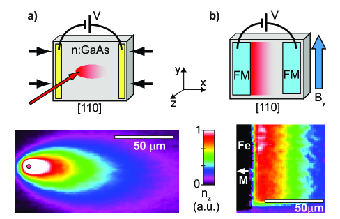
FIG. 1.: Diagrams and corresponding experimental data of the two measurement geometries considered in this work. (a) Spin polarized electrons, oriented along $\hat{z}$, are optically injected into an n:GaAs epilayer with a focused, circularly polarized laser incident along the z-axis (indicated by the red arrow). Lateral contacts provide an in-plane electric field (${\bf E}\parallel\pm\hat{x}$), Helmholtz coils provide an in-plane magnetic field (${\bf B}\parallel\pm\hat{y}$), and off-diagonal strain $\epsilon_{xy}$ results from controlled uniaxial stress applied along the [110] GaAs crystal axis. Scanning polar Kerr-rotation microscopy is used to spatially image $n_{z}$, the z-component of the resulting steady-state electron spin polarization. The drift, diffusion and precession of the spin flow are determined (in part) by the applied electric, magnetic and strain fields (see data below; adapted from Ref. [15]). (b) Electrical injection of spin-polarized electrons into an n:GaAs epilayer using ferromagnetic (FM) injector contacts. The contact magnetization (M) may be either in the x-y plane, or out-of-plane (M$\|\hat{z}$). As shown schematically, the injected spins then flow laterally within the n:GaAs epilayer, and $n_{z}$ can be spatially imaged with scanning Kerr microscopy. Experimental data, using an iron injector with M$\|-\hat{x}$ and $B_{y}=3.6$ G is shown below (adapted from Ref. [16]).

To theoretically describe the effects of spin-strain coupling, we consider a Hamiltonian of the form

$$H=\frac{1}{2m}[{\bf p}-\frac{e}{c}{\bf A}({\bf R})]^{2}+e\phi({\bf R})+\frac{\hbar}{2}\mbox{\boldmath$\Omega$}^{eff}\cdot\mbox{\boldmath$\sigma$},$$ (1)

$$\mbox{$\hbar$ \boldmath$\Omega$}^{eff}=g\mu_{B}{\bf B}+C_{3}\mbox{\boldmath$\varphi$}\ .$$ (2)

(Details of our microscopic treatment, that also include Dresselhaus [38] and Rashba [39] spin coupling terms, are described in the Appendix.) Here $\sigma$ is the vector having the three Pauli spin matrices as its components, $e=-|e|$ is the charge of an electron, $m$ is the conduction electron effective mass, $\phi$ is the scalar potential, $g$ is the conduction electron gyromagnetic ratio, $\mu_{B}$ is the Bohr magneton, $\bf B$ is the applied magnetic field and ${\bf A}$ is the corresponding vector potential. The term

$$\varphi_{x}=(\epsilon_{xy}k_{y}-\epsilon_{xz}k_{z}),$$ (3)

where $\varphi_{y}$ and $\varphi_{z}$ are obtained by cyclic permutations, describes the lowest-order $\bf k$-linear coupling of electron spin to the off-diagonal components of the crystal strain tensor[40]. Here, $\epsilon_{ij}$ is the strain tensor,

$\displaystyle C_{3}=\frac{4}{3}\hbar\frac{C_{2}\eta}{\sqrt{2E_{g}m(1-\eta/3)}}\ ,\ \ \ \eta=\frac{\Delta}{E_{g}+\Delta}\ ,$

$C_{2}$ is the interband deformation potential constant for acoustic phonons, $\Delta$ is the spin-orbit splitting of the valence band and $E_{g}$ is the band gap energy. For electrons moving laterally in the x-y sample plane, the spin-strain coupling term takes the form $\epsilon_{xy}(\sigma_{x}k_{y}-\sigma_{y}k_{x})$, which has the same form as the Rashba spin coupling in asymmetric heterostructures. That is, the presence of off-diagonal strain results in an effective magnetic field B_ϵ which is in-plane, orthogonal to the electron momentum k, and grows linearly with the magnitude of k. In contrast, spin-magnetic field coupling is independent of k. Because of this difference, strain and magnetic fields affect the flow of spin-polarized electrons in qualitatively different ways.

We derive spin-drift-diffusion equations for the spin density matrix

$$\rho_{s}=n({\bf R})+\sum_{i=x,y,z}n_{i}({\bf R})\sigma_{i},$$ (4)

accounting for the quantum nature of spin. Here $n$ is the total electron density and $n_{i}$ denote the three spin density components. Information about spin polarization along any given direction $\hat{s}$ is found by Tr$\rho_{s}\sum_{i=x,y,z}s_{i}\sigma_{i}$. We consider a case, corresponding to the experimental geometry, in which the net electron density is position independent and the electric, magnetic and strain fields are uniform. As shown in the Appendix, for electric and magnetic fields in the x-y plane and stress along a [110] crystal axis, the system of spin-drift-diffusion equations for the spin density matrix is given by

$$\left(D\nabla_{\bf R}^{2}+\mu{\bf E}\cdot\nabla_{\bf R}-C_{s}^{2}D-\frac{1}{\tau_{s}}\right)n_{x}$$ (5)

$$-\left[-C_{B_{y}}-C_{s}\left(2D\frac{\partial}{\partial x}+\mu E_{x}\right)\right]n_{z} = -G_{x}({\bf R}),$$ (6)

$$\left(D\nabla_{\bf R}^{2}+\mu{\bf E}\cdot\nabla_{\bf R}-C_{s}^{2}D-\frac{1}{\tau_{s}}\right)n_{y}\ \ \$$ (7)

$$-\left[C_{B_{x}}-C_{s}\left(2D\frac{\partial}{\partial y}+\mu E_{y}\right)\right]n_{z} = -G_{y}({\bf R}),$$ (8)

$$\left(D\nabla_{\bf R}^{2}+\mu{\bf E}\cdot\nabla_{\bf R}-2C_{s}^{2}D-\frac{1}{\tau_{s}}\right) n_{z}$$ (9)

$$+\left[-C_{B_{y}}-C_{s}\left(2D\frac{\partial}{\partial x}+\mu E_{x}\right)\right]n_{x}$$ (10)

$$+\left[C_{B_{x}}-C_{s}\left(2D\frac{\partial}{\partial y}+\mu E_{y}\right)\right]n_{y} = -G_{z}({\bf R}),$$ (11)

where $\tau_{s}$ is the spin relaxation time, $D$ is the electron diffusion coefficient, $\mu$ is the electron mobility, $C_{s}=C_{3}m\epsilon_{xy}/\hbar^{2}$, $\hbar C_{B_{i}}=g\mu_{B}B_{i}$ ($i=x,y$) and the vector $\bf G$ describes generation of the spin components. Because the spin-strain coupling depends on electron wave vector, both $D$ and $\mu$ appear in the strain coupling terms. $D$ and $\mu$ do not appear in the magnetic field coupling terms. A second order term in strain, $C_{s}^{2}D$, appears in the drift diffusion equations. The analogous second order term in magnetic field is proportional to the momentum relaxation time, which is short on the time scales of interest here, and thus this term is very small and can be neglected (see the Appendix for details.)

Performing a 2-D Fourier transform to momentum space, the system of equations for the spin polarization components, in our experimental geometry, is given by

$$O_{1}({\bf q})n_{x}({\bf q})+O_{2}({\bf q})n_{z}({\bf q}) = -G_{x}({\bf q})\ ,$$ (12)

$$O_{1}({\bf q})n_{y}({\bf q})+O_{3}({\bf q})n_{z}({\bf q}) = -G_{y}({\bf q})\ ,$$ (13)

$$O_{4}({\bf q})n_{z}({\bf q})-O_{2}({\bf q})n_{x}({\bf q})-O_{3}({\bf q})n_{y}({\bf q}) = -G_{z}({\bf q}),$$ (14)

where

$$O_{1}({\bf q}) = \left[-Dq^{2}+i\mu{\bf E}\cdot{\bf q}-C_{s}^{2}D-\frac{1}{\tau_{s}}\right]\,$$ (15)

$$O_{2}({\bf q}) = [C_{B_{y}}+C_{s}(i2Dq_{x}+\mu E_{x})]\ ,$$ (16)

$$O_{3}({\bf q}) = -[C_{B_{x}}-C_{s}(i2Dq_{y}+\mu E_{y})]\ ,$$ (17)

$$O_{4}({\bf q}) = \left[-Dq^{2}+i\mu{\bf E}\cdot{\bf q}-2C_{s}^{2}D-\frac{1}{\tau_{s}}\right].$$ (18)

The resulting spin density, $n_{i}({\bf R})$, is then given by the 2-D Fourier transform of $n_{i}({\bf q})$,

$$n_{i}({\bf R})=\frac{1}{2\pi}\int e^{i{\bf q}\cdot{\bf R}}n_{i}({\bf q})d^{2}{\bf q}.$$ (19)

The solutions for the spin polarization components from this system of equations are

$$n_{x}({\bf q})=\frac{-(O_{4}+\frac{{O_{3}}^{2}}{O_{1}})G_{x}+(\frac{O_{2}O_{3}}{O_{1}})G_{y}+O_{2}G_{z}}{d},$$ (20)

$$n_{y}({\bf q})=\frac{(\frac{O_{2}O_{3}}{O_{1}})G_{x}-(O_{4}+\frac{{O_{2}}^{2}}{O_{1}})G_{y}+O_{3}G_{z}}{d},$$ (21)

$$n_{z}({\bf q})=-\frac{O_{2}G_{x}+O_{3}G_{y}+O_{1}G_{z}}{d},$$ (22)

where the denominator, $d$, is

$$d=O_{1}O_{4}+(O_{2})^{2}+(O_{3})^{2}.$$ (23)

In Fig. 2 we compare our calculations with experimental results for the case of optical spin injection. These experimental data were obtained via scanning Kerr microscopy [15]. In these measurements, a linearly polarized narrowband Ti:sapphire laser, tuned just below the GaAs band-edge and focused to a 4 $\mu$m spot on the sample surface, was raster-scanned in the x-y sample plane to construct a 2-D image of $n_{z}$, the z-component of the electron spin density. The sample was a Si-doped n-type GaAs epilayer (electron density = $1\times 10^{16}$ cm^-3) grown on a [001] oriented semi-insulating GaAs substrate. Spin polarized electrons were optically injected into the sample by a separate, circularly-polarized 1.58 eV diode laser that was also focused to a 4 $\mu$m spot on the sample. Measurements were performed at a temperature of 4 K. For additional experimental details, see Ref.[15]. Figures (a), (c), and (e) compare calculated and measured results for spin flowing to the right in the presence of uniform off-diagonal strain ($\epsilon_{xy}=4\times 10^{-4}$; $E_{x}=12$ V/cm), while Figs. (b), (d), and (f) compare calculated and measured results for spins flowing to the right in the presence of an applied magnetic field ($B_{y}=16$ G; $E_{x}=7$ V/cm). There is very good agreement between theory and experiment. The material parameters used in the calculation were: mobility $\mu=3000$ cm²/Vs, spin relaxation time $\tau_{s}=125$ ns (we use these values for $\mu$ and $\tau_{s}$ throughout the paper), and diffusion constant $D=10$ cm²/s. Throughout the paper we use a value of $C_{3}=4.0$ eVÅ  for the spin-strain coupling coefficient based on the experiments of Ref. [41]. Both strain and magnetic field lead to precession of the electron spins. However, the spatial damping of the precession is more pronounced when magnetic rather than strain fields are applied (at the same precession length). In the remainder of the paper, we discuss various predictions of the spin-drift-diffusion model.

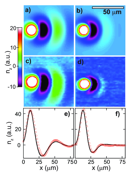
FIG. 2.: (a) and (b) show images of the calculated z-component of electron spin density ($n_{z}$) for optically injected spins that are flowing to the right and that are subject to (a) applied [110] stress (strain $\epsilon_{xy}=4\times 10^{-4}$; $E_{x}=12$ V/cm), and (b) applied magnetic field ($B_{y}=16$ G; $E_{x}=7$ V/cm). Note that the color scale is modified such that black indicates negative values of $n_{z}$ (i.e., spins that have precessed into the sample plane). For all calculations, $D=10$ cm²/s, $\mu=3000$ cm²/Vs, and $\tau_{s}=125$ ns. (c) and (d) show images of corresponding experimental data under the same conditions. (e) and (f) directly compare line cuts through the center of the corresponding calculated (black line) and measured (red dots) images.

III Contrasting the effects of magnetic and strain fields

Although strain and magnetic fields both lead to electron spin precession, spin precession due to strain differs qualitatively from that due to a magnetic field because spin-strain coupling depends linearly on the electron wave vector ${\bf k}$ whereas spin-magnetic field coupling is independent of electron wave vector. For spin precession in an applied magnetic field there is a pronounced spatial dephasing of spin precession due to the randomizing nature of diffusion. The net spin polarization at a remote location from the point of spin generation results from the combined sum of many random walk paths. Each path takes a different amount of time, giving a different precession angle. As a result the spatial coherence of the spin flow is rapidly lost. By contrast, the spin precession frequency in a strain field scales linearly with the electron wave vector. As a result the precession angle is correlated with electron velocity and therefore with the electron’s position. There is a partial cancelation of accumulated precession angle during the parts of the diffusive path that are traversed in the opposite direction, due to the linear dependence of effective magnetic field on electron momentum. Indeed, for motion strictly in one dimension, the spin ensemble would not dephase at all (however, it would still decohere with a timescale $\tau_{s}$). Scattering from $+\textbf{k}$ to $-\textbf{k}$ simply reverses the direction of precession, leading to an exact correspondence between spatial position and spin orientation.

A second difference between spin precession due to strain and that due to magnetic field is that for spin-magnetic field coupling the spatial precession length increases with increasing electric field (drift velocity), whereas for spin-strain coupling this length scale is independent of electric field. For spin-magnetic field coupling, the spin precession frequency is independent of electric field, but because the electrons drift faster in a larger electric field, the spatial precession length increases. For spin-strain coupling, the precession frequency scales directly with the average electron velocity, so that the spatial spin precession length is nearly independent of electric field.

To illustrate these differences, we consider the simple geometrical case in which spins are generated by a stripe optical excitation along the y-axis, the electric field ${\bf E}\parallel\hat{x}$, the magnetic field ${\bf B}\parallel\hat{y}$ and off-diagonal strain $\epsilon_{xy}$ is generated by stress applied along $\hat{x}$ (a [110] crystal axis). For this geometry, spin-drift-diffusion occurs along the x-axis so that the spin densities do not depend on the y-coordinate. Because of the orientation of strain and magnetic field, $n_{y}$ vanishes. For this geometrical case, $O_{3}$ vanishes and only the x-component, $q_{x}$, is of interest. The Green’s function for the z-component of spin density precesses and decays exponentially as $g_{z}(x)=A\exp(\eta\frac{x}{\sqrt{D\tau_{s}}})+CC$. The four complex decay parameters, $\eta$, can be found from the four zeros of the denominator $d$ in Eq. (18), $\eta=iq_{x}\sqrt{D\tau_{s}}$, where $q_{x}$ is a zero of $d$. Setting $\alpha={\mu E_{x}\tau_{s}}/{\sqrt{D\tau_{s}}}$, $\beta_{B}=C_{B_{y}}\tau_{s}$, $\beta_{s}=C_{s}\sqrt{D\tau_{s}}$, $Q=(\frac{\alpha}{2})^{2}+1$, and $\zeta=\eta+\frac{\alpha}{2}$, the zeros of $d$ are given by

$$[{\zeta}^{2}-(Q+{\beta_{s}}^{2})][{\zeta}^{2}-(Q+2{\beta_{s}}^{2})]=-[-\beta_{B}+2\beta_{s}\zeta]^{2}.$$ (24)

For strictly 1-D motion, in which the electrons are constrained to move only along the x-axis, the spin-drift-diffusion equations are modified in that the factor of 2 multiplying ${C_{s}}^{2}D$ in Eq. (6) is replaced by unity [see Eq. (48)]. The corresponding factor of 2 that appears in $O_{4}(\bf q)$, Eq. (13), and that multiplies ${\beta_{s}}^{2}$ in the second factor on the left hand side of Eq. (19) are also replaced by unity for this strictly 1-D case. The magnetic field terms of the spin-drift-diffusion equations are the same for the 1-D and 2-D cases.

We consider the solutions of Eq. (19) for three cases: (1) applied magnetic field without strain; (2) strain without magnetic field; and (3) strain without magnetic field for strictly 1-D motion. For case (1) the solutions are,

$$\zeta=\pm\sqrt{\frac{\sqrt{Q^{2}+{\beta_{B}}^{2}}+Q}{2}}\pm i\sqrt{\frac{\sqrt{Q^{2}+{\beta_{B}}^{2}}-Q}{2}}.$$ (26)

For case (2) the solutions are,

$$\zeta=\pm\sqrt{\frac{\sqrt{Q+{\beta_{s}}^{2}}\sqrt{Q+2{\beta_{s}}^{2}}+(Q-\frac{{\beta_{s}}^{2}}{2})}{2}}$$ (27)

$$\pm i\sqrt{\frac{\sqrt{Q+{\beta_{s}}^{2}}\sqrt{Q+2{\beta_{s}}^{2}}-(Q-\frac{{\beta_{s}}^{2}}{2})}{2}}.$$ (28)

For case (3) the solutions are,

$$\zeta=\pm\sqrt{Q}\pm i\beta_{s}.$$ (29)

From Eq. (20) we see that the real part of $\zeta$ increases with increasing magnetic field so that the decay length for spin density decreases with increasing magnetic field. From Eq. (21), we see that the real part of $\zeta$ also increases with increasing strain, but that there is a partial cancellation, due to the appearance of the term $-\frac{{\beta_{s}}^{2}}{2}$. The decay length for spin polarization also decreases with increasing strain, but more slowly than for magnetic field. To compare the strain and magnetic field cases, we consider strains and magnetic fields that give the same spatial precession length. For the case of strain in strictly 1-D motion, the factor of 2 and of $1/2$ that appear in the numerator of Eq. (21) are both replaced by unity and the partial cancelations that occur for the 2-D case become complete in the 1-D case, giving the result of Eq. (22). In this case strain does not reduce the decay length of spin polarization.

In Fig. 3, we calculate $n_{z}$ as a function of position for a narrow stripe excitation. The solid curve, which is the same in each of the panels, is for the non-precessing case of electric field only, with neither strain nor magnetic field. The dashed lines in the upper row show the case of applied magnetic field. The dashed lines in the center row show the case of applied strain, and the dashed lines in the lower row show the case of applied strain for strictly 1-D motion. If there is no strain, Eqs. (4)-(6) for the strictly 1-D motion case are the same as the 2-D case. The values of magnetic field and strain were chosen so that the spatial precession periods are approximately equal for the two cases. The values of strain and magnetic field in the right column of Fig. 3 are twice that in the left column. Comparing the solid and dashed lines in the upper row of Fig. 3 shows that $n_{z}$ decreases significantly when a magnetic field is applied. When the magnetic field is increased, the decay length is shorter. When strain is applied instead of magnetic field, as in the center row of Fig. 3, $n_{z}$ also decays more rapidly. However, the decay length remains longer for the case of strain than for the case of an equivalent magnetic field. When strain is applied for the case of strictly 1-D motion, the decay length is unchanged. The accumulated spin-precession angle due to strain depends only on the electron’s location and not on the path taken to reach that location, resulting in no dephasing of the ensemble spin-polarization. This behavior does not occur for strictly 1-D motion with magnetic field.

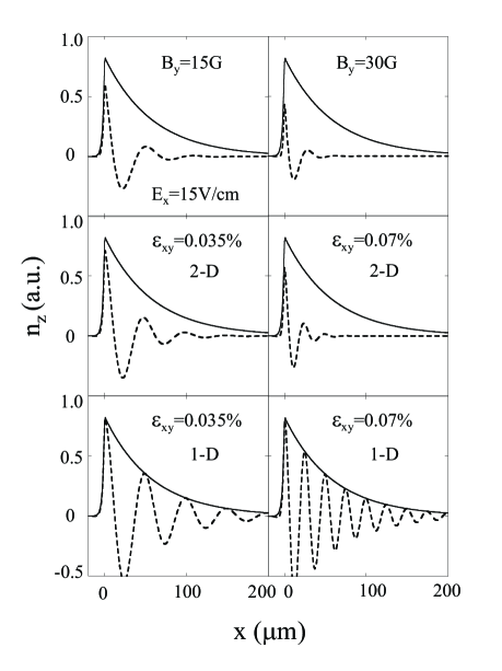
FIG. 3.: Calculated z-component of spin polarization ($n_{z}$) generated by a narrow stripe excitation at $x=0$ under the influence of a fixed electric field of $E_{x}=15$ V/cm and: Top row, a magnetic field of $B_{y}=15$ G (left) or $B_{y}=30$ G (right); center and lower rows, strain $\epsilon_{xy}=3.5\times 10^{-4}$ (left) or $\epsilon_{xy}=7\times 10^{-4}$ (right). The solid line is for electric field alone, without magnetic field or strain. The dashed lines represent cases where, in addition to the electric field, a magnetic or strain field is applied. The bottom row is for the case of strain and strictly 1-D motion. $D=10$ cm²/s, $\mu=3000$ cm²/Vs, and $\tau_{s}=125$ ns.

In Fig. 4, we compare the effect of increasing the electric field while in the presence of either a fixed magnetic field or a fixed off-diagonal strain. The geometry and material parameters are the same as for Fig. 3. The two panels in the left column show calculated results for $B_{y}=15$ G and $E_{x}=10$ V/cm (top panel) and $E_{x}=20$ V/cm (bottom panel). The two panels in the right column show calculated results for a strain of $\epsilon_{xy}=3.5\times 10^{-4}$ and the same electric fields as in the left column. Comparing the top and bottom panels in the left column, we see that for fixed applied magnetic field the spatial precession period increases with increasing electric field. By contrast, comparing the top and bottom panels in the right column, we see that for fixed strain the spatial precession period does not change with increasing electric field. This behavior was observed in Ref. [15]. For both strain and magnetic field, the spatial decay length increases as the electric field increases, due to the fact that spin transport is governed more by drift than by diffusion.

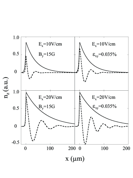
FIG. 4.: Calculated z-component of spin polarization ($n_{z}$) generated by a narrow stripe excitation at $x=0$ under the influence of a lateral electric field $E_{x}=10$ V/cm (top row) and $E_{x}=20$ V/cm (bottom row). $B_{y}=15$ G in the left column; $\epsilon_{xy}=3.5\times 10^{-4}$ in the right column. The solid line is for electric field alone, without magnetic field or strain (no precession). The dashed lines represent cases where, in addition to the electric field, a magnetic field or strain is present. $D=10$ cm²/s, $\mu=3000$ cm²/Vs, and $\tau_{s}=125$ ns.

IV Predictions of the Spin-Drift-Diffusion Model

In this section we present specific examples and predictions of the spin-drift-diffusion model. We first consider geometries that correspond to optical spin injection (initial spin density ${\bf n}_{0}\parallel\hat{z}$), and then consider geometries that correspond to electrical spin injection (${\bf n}_{0}\parallel\hat{x}$, with spatially extended source contacts).

Figure 5 shows the deleterious effect of diffusion on the spatial coherence of precessing spin flows. A steady-state spin polarization ${\bf n}_{0}\parallel\hat{z}$ is generated by a Gaussian source term with 4 $\mu$m full-width at half-maximum (FWHM), similar to the case of local optical spin injection. Spin-polarized electrons diffuse, and drift to the right in the presence of a lateral electric field, $E_{x}=10$ V/cm. We compare and contrast spin flows in the case of small diffusion constant (left column; $D=1$ cm²/s) with the case of large diffusion constant (right column; $D=20$ cm²/s). In Fig. 5(a) and (b), there is no applied magnetic field and no effective magnetic field due to strain, therefore the spin density $n_{z}$ decays monotonically away from the point of injection. The larger diffusion constant in Fig. 5(b) is reflected in the greater diffusive spread of spin polarization along the y-axis. In Figs. 5(c) and (d) there is an additional magnetic field ($B_{y}=20$ G), and the spins now precess as they flow to the right. With increasing distance from the point of spin injection, many spin precession cycles are observed when the diffusion constant is small (Fig. 5c). In contrast, only a single full precession cycle is visible when the diffusion constant is large (Fig. 5d). These images directly reveal how the effects of an increased diffusion constant can lead to significant spatial dephasing of precessing spin flows. Figures 5(e) and (f) show the spin flow precessing in the presence of an effective magnetic field due to strain ($\epsilon_{xy}=7\times 10^{-4}$). Again, the degree of spatial spin coherence is much higher when the diffusion constant is smaller. Further, the line-cuts in Figs. 5 (g) and (h) show that the degree of spatial spin coherence is better maintained for the case of strain than for the case of magnetic field, as discussed in section III.

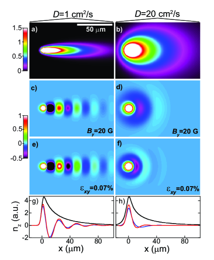
FIG. 5.: Calculated 80 x 120 $\mu$m images of $n_{z}$ for optically-injected spins, showing how diffusion directly influences the degree of spatial spin coherence for precessing spin flows. Images in the left column are for $D=1$ cm²/s; images in the right column are for $D=20$ cm²/s. All calculations use $E=10$ V/cm, $\mu=3000$ cm²/Vs, and $\tau_{s}=125$ ns. (a) and (b) show spin flow in the absence of magnetic or strain fields. (c) and (d) show precessing spin flow in the presence of $B_{y}=20$ G. (e) and (f) show precessing spin flow in the presence of strain ($\epsilon_{xy}=7\times 10^{-4}$). (g) and (h) show line-cuts through the center of the corresponding images, with blue and red lines showing the case of finite $B_{y}$ and $\epsilon_{xy}$, respectively.

Figure 6 shows how the effective magnetic field due to strain (${\bf B}_{\epsilon}$) can either augment or oppose a real magnetic field ($B_{y}$), leading to markedly different spin flows depending on the flow direction. The schematic diagrams at the top of Fig. 6 illustrate how a uniform applied magnetic field $B_{y}$ is vectorially summed with the effective magnetic field ${\bf B}_{\epsilon}$ due to finite strain, for the case of spin polarized electrons diffusing radially away from the point of injection (no drift). Since ${\bf B}_{\epsilon}$ is always orthogonal to electron momentum k, ${\bf B}_{\epsilon}$ is chiral for radially-diffusing spins, as shown. Under the conditions of Fig. 6, the vector sum of these two fields is given by ${\bf B}_{net}$, which is finite for spins diffusing to the left, and negligible for spins diffusing to the right. In Fig. 6(a), spin polarization ${\bf n}_{0}\parallel\hat{z}$ is generated by a 4 $\mu$m Gaussian FWHM source term, the applied field $B_{y}=6$ G, and the strain is $\epsilon_{xy}=2\times 10^{-4}$. Spin polarized electrons are subject to diffusion only ($E_{x}=0$). The resulting image of $n_{z}$ is completely asymmetric – spins diffusing to the left “see” a net magnetic field and precess, while electrons diffusing to the right experience negligible net magnetic field and do not precess. This behavior was observed in Ref. [15]. The asymmetry is even more apparent when the spins drift in the presence of a lateral electric field ${\bf E}\parallel\pm\hat{x}$. Fig. 6 (b) shows that spins flowing to the left ($E_{x}=-10$ V/cm) exhibit pronounced precession with many precession cycles, while Fig. 6 (c) shows that spins flowing to the right under the opposite lateral bias ($E_{x}=+10$ V/cm) do not precess ($B_{y}$ and ${\bf B}_{\epsilon}$ effectively cancel in this direction, under these conditions). Fig. 6 (d) shows corresponding line-cuts through the images.

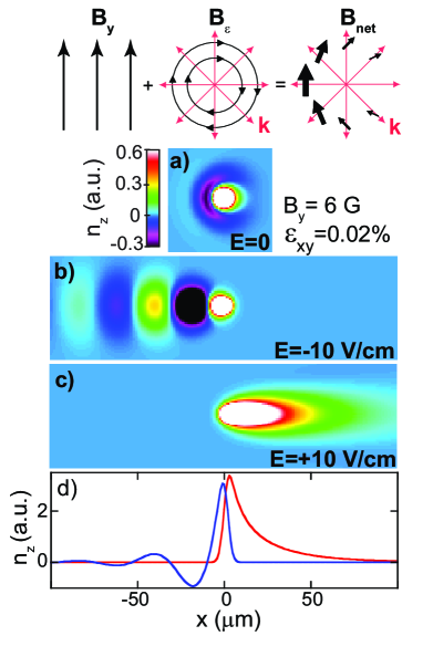
FIG. 6.: Diagram and calculated images showing how an effective magnetic field due to off-diagonal strain (${\bf B}_{\epsilon}$) can either augment or oppose a real magnetic field $B_{y}$, depending on the electron momentum k. (a) Calculated 60 x 60 $\mu$m image of spin diffusion with no electric field, and with $B_{y}=6$ G and strain $\epsilon_{xy}=2\times 10^{-4}$. Spins diffuse radially away from the point of injection, “sampling” all momenta k in the x-y plane. Spins diffusing to the left see a net effective magnetic field and precess; spins diffusing to the right see negligible net effective magnetic field and do not precess. (b) With $E_{x}=-10$ V/cm, electrons flowing to the left show pronounced spatial precession. (c) With $E_{x}=+10$ V/cm, electrons flowing to the right show essentially no precession. (d) Corresponding line-cuts through the center of the images in (b) and (c). In all images, $D=3$ cm²/s, $\tau_{s}=125$ ns, and $\mu=3000$ cm²/Vs.

The spin drift-diffusion equations [Eqs. (15) - (18)] can also be used to compute the in-plane components of electron spin polarization ($n_{x}$ and $n_{y}$). Knowledge of $n_{x}$ and $n_{y}$ is useful for comparison with experiments that are directly sensitive to in-plane components of electron spins, such as longitudinal or transverse (as opposed to polar) magneto-optical Kerr effect studies, or for direct electrical measurement of in-plane electron spin using ferromagnetic electrical drain contacts that exhibit a spin-sensitive conductance [16]. Figure 7 demonstrates the utility of Eqs. (15)-(18) by computing all three components of electron spin polarization ($n_{z}$, $n_{x}$, and $n_{y}$) for the case of optically injected electrons (${\bf n}_{0}\parallel\hat{z}$) diffusing in the presence of both a real uniform magnetic field $B_{y}$ (left column), and in the presence of an effective chiral magnetic field due to strain ${\bf B}_{\epsilon}$ (middle column). The rightmost column shows horizontal line-cuts through the center of the corresponding images of $n_{z}$ and $n_{x}$. The diagrams at the bottom of Fig. 7 illustrate how electron spins, generated at the center of the image, precess from initially out-of-plane (${\bf n}_{0}\parallel\hat{z}$) to an in-plane direction as they diffuse. In the case of a uniform applied magnetic field $B_{y}$, all electrons precess in the same direction about $B_{y}$ regardless of their momentum, so that $n_{x}$ is finite with circular symmetry, and $n_{y}$ is everywhere zero. In contrast, electrons diffusing in the presence of strain precess about the chiral effective magnetic field ${\bf B}_{\epsilon}$ such that their spins are oriented radially away from the point of injection (at some characteristic radial distance). This radial spin distribution is reflected in the asymmetric images of $n_{x}$ and $n_{y}$. In the presence of strain, the fact that the sign of electron spin polarization (for a spin component orthogonal to the spin generation term) is dependent on the direction of spin flow has been shown to be a valuable diagnostic tool (see Ref. [16]).

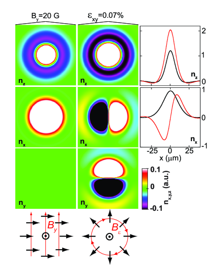
FIG. 7.: 40 x 40 $\mu$m images of the calculated z-, x-, and y-components of optically-injected spin polarization ($n_{z},n_{x},n_{y}$). Spins are injected with ${\bf n}_{0}\parallel\hat{z}$ at the center of the images, and subject to diffusion only (no electric field) in the presence of either an applied magnetic field (left column; $B_{y}=20$ G), or strain (middle column; $\epsilon_{xy}=7\times 10^{-4}$). $D=10$ cm²/s and $\tau_{s}=125$ ns. The rightmost column shows horizontal line-cuts through the center of the corresponding images of $n_{z}$ and $n_{x}$. The diagrams at the bottom illustrate how spins precess from initially out-of-plane (${\bf n}_{0}\parallel\hat{z}$) to in-plane while diffusing in the uniform magnetic field $B_{y}$, or in the chiral effective magnetic field ${\bf B}_{\epsilon}$.

For electrical spin injection from ferromagnetic contacts, the generation source is usually spatially extended and the orientation of injected spins follows the contact magnetization, which is typically in the x-y plane of the sample surface. However, polar magneto-optical Kerr microscopy is sensitive to $n_{z}$, the z-component of spin polarization. Therefore, a magnetic or strain field must be used to rotate the injected spin polarization out-of-plane in order to allow detection. In Fig. 8, we show calculated images of $n_{z}$ resulting from a (theoretical) 40 $\mu$m wide ferromagnetic stripe contact having in-plane magnetization (M$\parallel\hat{x}$). This spin polarization source is analogous to the Fe/GaAs spin injection contacts used experimentally in Ref. [16]. The left column shows $100\times 200$ $\mu$m images of $n_{z}$, and the right column shows horizontal line-cuts through the images. In Fig. 8(a), electrons injected with initial spin orientation ${\bf n}_{0}\parallel\hat{x}$ diffuse in the presence of strain ($\epsilon_{xy}=1\times 10^{-4}$). Spins diffusing to the left and right precess into-plane and out-of-plane, respectively, giving the asymmetric image shown. The maxima and minima of $n_{z}$ nearly coincide with the edges of the source contact because the contact width greatly exceeds the characteristic spin diffusion length $\sqrt{D\tau_{s}}$. In Fig. 8(b), we consider the injected spins diffusing in the presence of a applied magnetic field ($B_{y}=1$ G). The image of $n_{z}$ is symmetric, because electrons precess in the same direction (out-of-plane) regardless of which way they diffuse. Lastly, Fig. 8(c) includes an additional uniform drift electric field ($E_{x}=4$ V/cm), which shifts the spin polarization in the direction of electron drift (we consider the simplest case here, in which electric field is uniform across the image; i.e., the electric field is not generated by the injection contact, nor does the injection contact distort the uniform electric field.) Note that finite spin polarization $n_{z}$ still exists on the “upstream” side of the source contact due to diffusion of injected electrons against the net electron current.

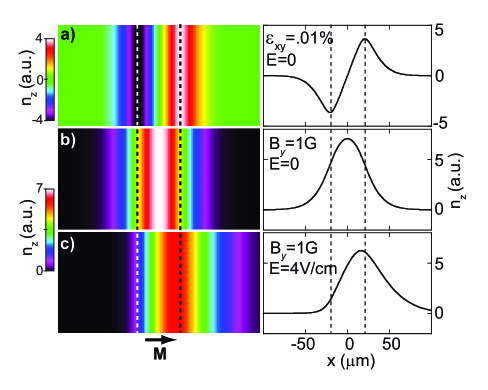
FIG. 8.: 100 x 200 $\mu$m images of the calculated z-component of electron spin polarization ($n_{z}$) resulting from in-plane spin injection (${\bf n}_{0}\parallel{\bf M}\parallel\hat{x}$) by a 40-$\mu$m wide magnetized stripe contact (edges of the stripe are shown by dashed lines). Corresponding horizontal line-cuts through the center of the images are shown to the right. (a) Spin diffusion alone for the case of a strained sample ($\epsilon_{xy}=1\times 10^{-4}$). Spins diffusing to the left or right precess in opposite directions. (b) Spin diffusion alone for the case of an applied magnetic field ($B_{y}=1$ G). (c) Spin diffusion and drift for the case of applied magnetic and lateral electric fields ($B_{y}=1$ G, $E_{x}=4$ V/cm). For all images, $\mu=3000$ cm²/Vs, $D=10$ cm²/s, $\tau_{s}=125$ ns.

Finally, we demonstrate the utility of the spin drift-diffusion equations in modeling the two-dimensional spin flows resulting from nontrivially-shaped injection sources (having either in-plane or out-of-plane magnetization), such as might be realized in actual experiments. Figure 9 shows calculated images of $n_{z}$ in a semiconductor epilayer resulting from a uniform square $80\times 80$ $\mu$m injection contact. In Fig. 9 (a) and (c), the contact magnetization (and injected spin polarization) is oriented out-of-plane (${\bf M}\parallel{\bf n}_{0}\parallel\hat{z}$). For comparison, the contact magnetization (and injected spin polarization) in Figs. 9 (b) and (d) is in-plane and along the x-axis (${\bf M}\parallel{\bf n}_{0}\parallel\hat{x}$). Spins drift to the right in an electric field of $E_{x}=8$ V/cm in all of the images.

In actual experiments, it is often desirable to measure the spin polarization $n_{z}$ at a specific location on the sample as a function of in-plane magnetic field $B_{y}$ [11, 16]. These “Hanle curves” [40] provide valuable information on the dynamics of the flowing spins, and in certain cases can be used to infer spin drift velocities and also, in conjunction with controlled strain, the direction of spin flow [16]. Figures 9(e) and (f) show calculated Hanle curves acquired at 4, 20, 40, and 80 $\mu$m from the right edge of the square injection contact. Solid (dashed) lines show the Hanle curves in the absence (presence) of strain. For the case of out-of-plane injection [Fig. 9 (e)], the Hanle curves are symmetric with respect to $B_{y}$. In contrast, for the case of in-plane injection [Fig. 9(f)], the Hanle curves are antisymmetric with respect to $B_{y}$, as expected for orthogonal spin generation and detection axes. Unlike conventional Hanle measurements which are typically sensitive to the spin polarization of all injected spins (e.g., the case of optical spin injection and detection via spatially-integrated luminescence polarization), in these studies the injection source and the point of detection may be spatially separated, so that only a subset of the injected electrons are detected by the probe laser. Further, these experiments allow access to a regime wherein the spin drift length exceeds the characteristic spin diffusion length. In this regime the Hanle curves can exhibit highly atypical shapes, even showing multiple oscillations as $B_{y}$ is swept [16]. For the images of Fig. 9, where the injected spins subsequently flow to the right, the effect of strain is to shift the Hanle curves to negative values of $B_{y}$ (dashed lines), implying that the effective magnetic field due to strain (${\bf B}_{\epsilon}$) is oriented along $+\hat{y}$. Conversely, a shifted Hanle curve can be used to infer the presence of strain in the sample, and also can be used (in conjunction with controlled strain) to infer the actual direction in which the spin polarized electrons are flowing [16].

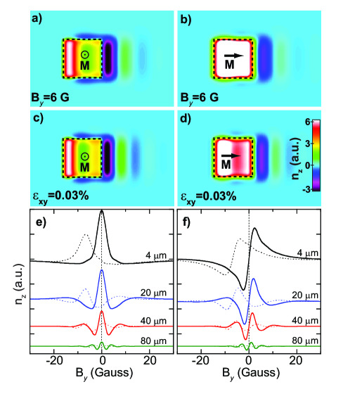
FIG. 9.: Calculated images of $n_{z}$ resulting from either out-of-plane (left column) or in-plane (right column) spin injection and subject to either magnetic or strain fields. The 300 x 200 $\mu$m images show the z-component of calculated electron spin polarization ($n_{z}$) resulting from a square 80 x 80 $\mu$m injection contact (edges of the source are indicated by dashed lines). In (a) and (c) the contact magnetization is out-of-plane (${\bf n}_{0}\parallel\hat{z}$), and in (b) and (d) the contact magnetization is in-plane (${\bf n}_{0}\parallel\hat{x}$). Measuring $n_{z}$ at a specific position as a function of in-plane magnetic field $B_{y}$ yields the “Hanle curves” [40] shown in (e) and (f). These curves are acquired at distances of 4, 20, 40 and 80 $\mu$m from the right edge of the square source contact. Solid lines correspond to sweeping $B_{y}$ alone; dashed lines include the presence of strain ($\epsilon_{xy}=0.03\%$), which shifts the Hanle curves to the left. In the calculations, $\mu=3000$ cm²/Vs, $E_{x}=8$ V/cm, $D=3$ cm²/s, and $\tau_{s}=125$ ns.

V Summary and Conclusion

We investigated the effects of electric fields, magnetic fields, and off-diagonal strain on the transport of spin-polarized electrons in zincblende semiconductors. Starting with a quantum kinetic approach, we first derived a semiclassical kinetic theory of electron spin dynamics and transport, and from this kinetic theory constructed spin-drift-diffusion equations when the total electron density is position independent and for spatially uniform electric, magnetic, and strain fields. This case of spatially uniform fields and uniform electron density corresponds to the experimental situation realized in Refs. [15] and [16]. We compared the results of our spin-drift-diffusion model with Kerr microscopy images and found very good agreement. Our semiclassical kinetic theory is formulated on a microscopic foundation and can be extended to the cases of spatially varying (electric, magnetic and strain) fields and electron density. We contrasted the spin precession resulting from magnetic and strain fields. We found that because spin-strain coupling depends linearly on electron wave vector whereas spin-magnetic field coupling is independent of electron wave vector k, spatial coherence of electron spin precession is much better maintained with strain than with magnetic fields. This effect is most dramatic for 1-D systems. In contrast to the case of a magnetic field, we find that the spatial period of electron spin precession is independent of the applied electrical bias in samples with off-diagonal strain. The freedom to operate at variable electric bias may benefit functional devices that are based on rotation of spin from one point in space to the other, as in spin transistor designs. Finally, we explore the utility of the spin drift-diffusion model by considering spin flows in a variety of potential cases, such as in-plane and out-of-plane spin injection from spatially extended sources in the presence of electric, magnetic, and/or strain fields.

VI Acknowledgment

The authors thank Lev Boulaevskii, Thomas Luu, Slobodan Matić, Paul Crowell, Chris Palmstrøm and Peter Littlewood for useful discussions and input. This work was supported by the Los Alamos National Laboratory LDRD program.

VII Appendix: Semiclassical Kinetic Theory of Electron Spin Dynamics with Electric, Magnetic and Strain Fields

We start from the Keldysh Green’s function description [42] for a system driven out of equilibrium [43]. The Dyson equation

$$(\hat{G}_{0}^{-1}-\hat{\Sigma})\otimes\hat{G}=\delta(1,2)$$ (30)

is written for the 4x4 matrix Green’s function in the tensor product of spin and Keldysh space

$$\hat{G}=\left(\begin{array}[]{cc}G^{R}&G^{K}\\ 0&G^{A}\end{array}\right),$$ (31)

where $G^{R}$, $G^{A}$ and $G^{K}$ are the retarded, advanced and Keldysh Green’s function which are 2x2 matrices in spin space (for more details on this Larkin-Ovchinnikov notation see Ref. [44]). The operator $\hat{G}_{0}^{-1}$ is defined as

$$\hat{G}_{0}^{-1}(1,2) = \left(\begin{array}[]{cc}G_{0}^{-1}&0\\ 0&G_{0}^{-1}\end{array}\right)\ ,$$ (34)

$$G_{0}^{-1} = [i\hbar\partial_{t_{1}}-\hat{\epsilon}(1)]\delta(1,2),$$ (35)

where the indices $1,2$ represent the first and the second set of coordinate, time and spin variables and $\delta(1,2)$ represents a product of delta-functions in these variables; the operation $\otimes$ denotes matrix product in relevant spaces. Here $\hat{\Sigma}$ is the self-energy operator while $\hat{\epsilon}$ expresses the effective mass Hamiltonian for the two spin states near the conduction band minimum. It is diagonal in Keldysh space and given by [40]

$$\hat{\epsilon} = \left(\begin{array}[]{cc}\epsilon&0\\ 0&\epsilon\end{array}\right)\ ,$$ (38)

$$\epsilon(1) = \frac{1}{2m}[{\bf p}_{\bf{x_{1}}}-\frac{e}{c}{\bf A}(1)]^{2}+e\phi(1)+\frac{\hbar}{2}\mbox{\boldmath$\Omega$ }^{eff}\cdot\mbox{\boldmath$\sigma$},$$ (39)

$$\mbox{$\hbar$ \boldmath$\Omega$}^{eff} = g\mu_{B}{\bf B}+C_{3}\mbox{\boldmath$\varphi$}+\frac{\alpha_{c}\hbar^{3}}{\sqrt{2m^{3}E_{g}}}\mbox{\boldmath$\kappa$}+\alpha(\mbox{\boldmath{$k$}}\times\mbox{\boldmath{$\hat{n}$}})\ .$$ (40)

The last term in $\mbox{\boldmath$\Omega$}^{eff}$ with the coefficient $\alpha$ is the Rashba term (for an asymmetric heterostructure with symmetry-breaking axis $\bf\hat{n}$), while

$$\kappa_{x}=k_{x}(k_{y}^{2}-k_{z}^{2})$$ (41)

is the Dresselhaus term arising from bulk inversion asymmetry, $\alpha_{c}=(4/3)(m/m_{cv})\eta/\sqrt{1-\eta/3}$, $m_{cv}$ determines an interband term quadratic in $\bf k$ and is related to the interaction of the conduction and valence bands with other bands. The components $\kappa_{y}$ and $\kappa_{z}$ are obtained by cyclic permutations of Eq. (26). From symmetry considerations alone [40, 45] $\mbox{\boldmath$\Omega$}^{eff}$ could also contain terms that couple spin to diagonal strain components, e.g., terms of the form $\xi_{z}=k_{z}(\epsilon_{xx}-\epsilon_{yy})$, etc. However, these terms only appear if spin-orbit mixing of states widely separated in energy is included [see Ref.[40] for more details] and therefore their numerical coefficients are small.

The Dyson equation gives an exact description of the system. However, it cannot be reduced to an expression involving equal-time Green’s functions which determine physical quantities, such as densities and particle currents, via the single-particle density matrix. Deriving the quantum-kinetic equation involves considering the difference of the Dyson equation and its conjugate,

$$[\hat{G}_{0}^{-1}-\hat{\Sigma}\stackrel{{\scriptstyle\otimes}}{{,}}\hat{G}]_{-}=0$$ (42)

and approximations including a gradient expansion and a quasiclassical approximation. (Here $[A\stackrel{{\scriptstyle\otimes}}{{,}}B]_{-}$ denotes a commutator of quantities $A$ and $B$ with respect to the operation $\otimes$.) We use a result due to Langreth [46] within the gradient expansion to obtain the kinetic equation for a gauge invariant distribution function.

To introduce the gradient expansion, we transform to a mixed Wigner representation:

$${\bf R}=\frac{{\bf r_{1}}+{\bf r_{2}}}{2},\ T=\frac{t_{1}+t_{2}}{2},\ {\bf r}={\bf r_{1}}-{\bf r_{2}},\ t=t_{1}-t_{2} \ .$$

After performing a Fourier transform with respect to relative coordinates $\bf r$ and $t$

$$\hat{G}(X,p)=\int dt\int d{\bf r}e^{-ip\cdot x}\hat{G}(X+x/2,X-x/2)\ ,$$ (43)

where $X=(T,{\bf R})$, $x=(t,{\bf r})$, $p=(\omega,{\bf p}/\hbar)$ and the dot product is given by $p\cdot x=-\omega t+{\bf p}\cdot{\bf r}/\hbar$, we represent the Fourier transform as a Taylor expansion expression involving products of those quantities in the Fourier transformed mixed representation:

$$(M\otimes N)(X,p)=e^{i(\partial_{X}^{M}\cdot\partial_{p}^{N}-\partial_{p}^{M}\cdot\partial_{X}^{N})/2}M(X,p)N(X,p)\ .$$ (44)

We defined the exclusive partial derivatives $\partial_{X}^{M}=(-\partial_{T},\nabla_{\bf R})$, $\partial_{p}^{M}=(-\partial_{\omega},\hbar\partial_{\bf p})$ acting only on the quantity M; the scalar product of derivatives amounts to $\partial_{X}\cdot\partial_{p}=-\partial_{T}\partial_{\omega}+\hbar\partial_{\bf R}\partial_{\bf p}$. In the mixed representation the operator $G_{0}^{-1}$ is given by

$$G_{0}^{-1}({\bf R};\omega,{\bf p}) = \hbar\omega-\frac{1}{2m}({\bf p}-\frac{e}{c}{\bf A})^{2}-e\phi({\bf R})$$ (46)

$$-\frac{\hbar}{2}\mbox{ \boldmath$\Omega$}^{eff}({\bf R};{\bf p})\cdot\mbox{ \boldmath$\sigma$}\ .$$

Using the gradient expansion Eq. (44), Eq. (42) is written as

$$0=[\hat{G}_{0}^{-1}-\hat{\Sigma}\stackrel{{\scriptstyle\otimes}}{{,}}\hat{G}]_{-}(T,{\bf R};\omega,{\bf p})=i[\hat{G}_{0}^{-1}-\hat{\Sigma},\hat{G}]_{p}-$$ (47)

$$[\frac{\hbar}{2}\mbox{\boldmath$\Omega$}^{eff}({\bf R};{\bf p})\cdot\sigma\odot\hat{1}+\hat{\Sigma}(T,{\bf R};\omega,{\bf p}),\hat{G}(T,{\bf R};\omega,{\bf p})]_{-},$$ (48)

where

$$[M,N]_{p} = \frac{1}{2}(\partial_{X}^{M}M\partial_{p}^{N}N-\partial_{p}^{M}M\partial_{X}^{N}N)$$ (50)

$$-\frac{1}{2}(\partial_{X}^{N}N\partial_{p}^{M}M-\partial_{p}^{N}N\partial_{X}^{M}M)$$

is the generalized Poisson bracket and $\odot$ denotes a tensor product.

Within the gradient approximation, we introduce gauge-invariant quantities as

$${\tilde{A}}(\Omega,{\bf P},{\tilde{\bf R}},{\tilde{T}})=A(\omega,{\bf p},{\bf R},T)$$ (51)

by a change of variables

$${\bf P}={\bf p}-\frac{e{\bf A}}{c}({\bf R},T),\ \Omega=\omega-(e/\hbar)\phi({\bf R},T)\ .$$ (52)

The relations between the derivatives in old and new coordinates are

$$\partial_{\bf R} = -\frac{e}{\hbar}\nabla\phi\partial_{\Omega}-\frac{e}{c}\sum_{i,j}\hat{e}_{j}\frac{\partial A_{i}}{\partial R_{j}}\partial_{P_{i}}+\partial_{\tilde{\bf R}},$$

$$\partial_{T} = -e\frac{\partial\phi}{\partial T}\partial_{\Omega}-\frac{e}{c}\frac{\partial{\bf A}}{\partial T}\cdot\partial_{\bf P}+\partial_{\tilde{T}},$$

and $\partial_{\bf p}=\partial_{\bf P},\ \partial_{\omega}=\partial_{\Omega}$, where ${\bf E}$ is the electric field. From these relations one can prove the identity connecting the generalized Poisson brackets in old and new coordinates [46]

$$[M,N]_{p}=[{\tilde{M}},{\tilde{N}}]_{P}+$$ (53)

$$\frac{e}{2}\{[{\bf B}\cdot(\nabla_{\bf P}^{\tilde{M}}{\tilde{M}}\times\nabla_{\bf P}^{\tilde{N}}{\tilde{N}})+{\bf E}\cdot(\partial_{\Omega}^{\tilde{M}}{\tilde{M}}\nabla_{\bf P}^{\tilde{N}}{\tilde{N}}-\nabla_{\bf P}^{\tilde{M}}{\tilde{M}}\partial_{\Omega}^{\tilde{N}}{\tilde{N}})]$$ (54)

$$-[N\leftrightarrow M]\}\ .$$ (55)

The generalized Poisson bracket in the new variables is given by

$$\frac{1}{\hbar}[\hat{G}_{0}^{-1},\hat{G}]_{P}=\partial_{T}\hat{G}+{\bf v}\cdot\partial_{\bf R}\hat{G}$$ (56)

$$+\frac{\hbar}{2}\sum_{i,j}\sigma_{i}([\partial_{P_{j}}\Omega_{i}^{eff},\partial_{R_{j}}\hat{G}]_{+}-[\partial_{R_{j}}\Omega_{i}^{eff},\partial_{P_{j}}\hat{G}]_{+}),$$ (57)

where ${\bf v}={\bf P}/m$ and $[A,B]_{+}$ denotes an anticommutator. The Dyson equation in gauge invariant form becomes

$$\{\partial_{T}+{\bf v}\cdot\partial_{\bf R}+e{\bf E}\cdot(\partial_{\bf P}+\frac{{\bf v}^{eff}}{\hbar}\partial_{\Omega})\}\hat{G}$$ (58)

$$+\frac{1}{2}\sum_{i}([\sigma_{i}\partial_{\bf P}\Omega_{i}^{eff},\partial_{\bf R}\hat{G}]_{+}-[\sigma_{i}\partial_{\bf R}\Omega_{i}^{eff},\partial_{\bf P}\hat{G}]_{+})$$ (59)

$$+\frac{e}{c}({\bf v}^{eff}\times{\bf B})\cdot\partial_{\bf P}\hat{G}+\frac{i}{2}[\mbox{\boldmath$\Omega$}^{eff}\cdot\mbox{\boldmath$\sigma$},\hat{G}]_{-}=-i[\hat{\Sigma},\hat{G}]_{-},$$ (60)

where ${\bf v}^{eff}={\bf v}-(\hbar/2)\sigma_{i}\partial_{\bf P}\Omega_{i}^{eff}$. Equation  (60) is a central result of our microscopic derivation. It describes spin dynamics in the presence of electric, magnetic and strain fields provided the lengthscale of spatial variation is large compared to the characteristic lengthscale for wavefunction variation. For the case of uniform strain, the strain terms in Eq. (60) agree with those found in Ref.[35]. In the absence of strain fields, the half-sum of the $R$, $A$ and $K$ components of Eq.  (60) in the equal-time limit yields the kinetic equation obtained in Ref. [27] for the distribution function $N=-(i/2)(G^{K}+G^{R}-G^{A})$ [43].

The diagonal components $G^{R}$ and $G^{A}$ of the Green’s function characterize the states, while the Keldysh component $G^{K}$ contains information on the occupation of these states [44]. We consider the Keldysh component of Eq.  (60) in order to derive the kinetic equation. A distribution function $f(T,{\bf R};\Omega,{\bf P})$ is introduced by the ansatz

$$G^{K}=G^{R}\otimes f-f\otimes G^{A}\ .$$ (61)

Using $[G_{0}^{-1}-\Sigma^{R}\stackrel{{\scriptstyle\otimes}}{{,}}G^{R}]_{-}=0$ and $[G_{0}^{-1}-\Sigma^{A}\stackrel{{\scriptstyle\otimes}}{{,}}G^{A}]_{-}=0$, the Keldysh component of Eq.  (60) gives

$$G^{R}\otimes B-B\otimes G^{A}=0\ ,$$ (62)

where the $2\times 2$ matrix $B$ is given by

$$B[f] = [G_{0}^{-1}\stackrel{{\scriptstyle\otimes}}{{,}}f]_{-}-\Sigma^{R}\otimes f+f\otimes\Sigma^{A}+\Sigma^{K}$$ (63)

$$\equiv [G_{0}^{-1}\stackrel{{\scriptstyle\otimes}}{{,}}f]_{-}-C(\hat{\Sigma},f),$$ (64)

and in the mixed representation we have

$$-\frac{i}{\hbar}[G_{0}^{-1}\stackrel{{\scriptstyle\otimes}}{{,}}f]_{-}=i\frac{1}{2}[\mbox{\boldmath$\Omega$}^{eff}\cdot\mbox{\boldmath$\sigma$},f]_{-}$$ (65)

$$+\frac{\hbar}{2}\sum_{i}\left([\sigma_{i}\partial_{\bf P}\Omega_{i}^{eff},\partial_{\bf R}f]_{+}-[\sigma_{i}\partial_{\bf R}\Omega_{i}^{eff},\partial_{\bf P}f]_{+}\right)$$ (66)

$$+\{\partial_{T}+{\bf v}\cdot\partial_{\bf R}+e{\bf E}\cdot(\partial_{\bf P}+\frac{{\bf v}^{eff}}{\hbar}\partial_{\Omega})\}f,$$ (67)

where the Lorentz force term was neglected. In the geometry that we consider (Fig. 1), electrons are confined to move in a two-dimensional layer perpendicular to [001], and electric and magnetic fields are applied in the plane of electron motion. Hence the Lorentz force is along the z-axis and does not affect the motion in this case.

We seek the solution of Eq. (62) for the distribution function as the solution of the equation $B[f]=0$ i.e.

$$[G_{0}^{-1}\stackrel{{\scriptstyle\otimes}}{{,}}f]_{-}=C(\hat{\Sigma},f)\ .$$ (68)

Taking the equal-time limit (which amounts to integrating over $\Omega$ so that terms with derivative $\partial_{\Omega}$ vanish), Eq. (68) is then written as

$$\{\partial_{T}+{\bf v}\cdot\partial_{\bf R}+e{\bf E}\cdot\partial_{\bf P}\}h$$ (69)

$$+\frac{\hbar}{2}\sum_{i}([\sigma_{i}\partial_{\bf P}\Omega_{i}^{eff},\partial_{\bf R}h]_{+}-[\sigma_{i}\partial_{\bf R}\Omega_{i}^{eff},\partial_{\bf P}h]_{+})$$ (70)

$$+\frac{i}{2}[\mbox{\boldmath$\Omega$}^{eff}\cdot\mbox{\boldmath$\sigma$},h]_{-}=-\frac{i}{\hbar}\int d\Omega C(\hat{\Sigma},f),$$ (71)

where $h(T,{\bf R},{\bf P})=\int d\Omega f(T,{\bf R};\Omega,{\bf P})$.

For the experimental situation that we consider the applied electric, magnetic, and strain fields are spatially uniform and the net electron density is constrained by electrostatics to be spatially uniform. It is convenient to write $h={\rho_{0}+\sum_{i=1}^{3}\rho_{i}\sigma_{i}}$. For the steady state, spatially uniform case considered experimentally, Eq. (69) for the spin components of $\rho$ becomes a Boltzmann type equation of the form

$$\left\{\frac{{\bf P}}{m}\cdot\partial_{\bf R}+e{\bf E}\cdot\partial_{\bf P}\right\}{\rho}_{i}-[\mbox{\boldmath$\Omega$}^{eff}\times\mbox{\boldmath$\rho$}]_{i}={I^{i}}_{C},$$ (72)

where ${I^{i}}_{C}$ is a collision integral representing the right hand side of Eq. (69). To construct a spin-drift-diffusion equation from Eq. (72), we make the ansatz

$$\rho_{i}({\bf R},{\bf P})=n_{i}({\bf R})f^{0}({\bf P})+\delta_{i}({\bf R},{\bf P}),$$ (73)

where $n_{i}(\bf R)$ is a spin density that is to be determined, $f^{0}(\bf P)$ is a known equilibrium momentum distribution function and $\delta_{i}(\bf R,\bf P)$ is a small correction. The collision integral is described using a relaxation time approximation

$${I^{i}}_{C}=-\frac{\delta_{i}(\bf R,\bf P)}{\tau},$$ (74)

where $\tau$ is a momentum scattering time that may depend on $\bf P$ but not on $\bf R$. Substituting Eq. (73) into Eq. (72) and neglecting contributions for the correction term $\delta_{i}$ on the left hand-side gives a first approximation for $\delta_{i}$

$$\delta_{x}=-\tau\biggl{[}\left(\frac{\bf P}{m}\cdot\frac{\partial n_{x}}{\partial\bf R}\right)f^{0}+n_{x}\left(e{\bf E}\cdot\frac{\partial f^{0}}{\partial\bf P}\right)-$$ (75)

$$(\Omega^{eff}_{y}n_{z}-\Omega^{eff}_{z}n_{y})f^{0}\biggr{]}$$ (76)

with cyclic permutation of indices for the other components of $\delta_{i}$. This procedure can be iterated to give a systematic expansion for $\delta_{i}$, that is $\delta_{i}=\delta^{0}_{i}+\delta^{1}_{i}+...$ with the momentum scattering time $\tau$ being the small parameter in the expansion. We consider the case of rapid momentum scattering and keep only the lowest order term.

We integrate Eq. (72) over all momenta to give

$$\partial_{\bf R}\cdot\int d^{3}{\bf P}\left(\frac{{\bf P}}{m}{\rho}_{i}\right)+e{\bf E}\cdot\int d^{3}{\bf P}(\partial_{\bf P}{\rho}_{i})$$ (77)

$$-\int d^{3}{\bf P}[\mbox{\boldmath$\Omega$}^{eff}\times\mbox{\boldmath$\rho$}]_{i}=\int d^{3}{\bf P}({I^{i}}_{C})=(G_{i}-R_{i}).$$ (78)

The second term on the left-hand side of Eq. (77) vanishes identically and the possibility of spin generation ($G_{i}$) and relaxation ($R_{i}$) has been included empirically in the momentum integration of the scattering integral. [A more rigorous discussion of how momentum scattering (Elliot-Yafet mechanism) and the Dresselhaus term in the Hamiltonian (Dyakonov-Perel mechanism) lead to spin relaxation within this formal structure is given in Ref.[27].] Substituting Eq. (73) into Eq. (77) and using Eq. (75) for $\delta_{i}$, gives

$$-\partial_{\bf R}\cdot\int d^{3}{\bf P}\left(\frac{{\bf P}}{m}\right){\tau}\left[\left(\frac{{\bf P}}{m}\cdot\partial_{\bf R}n_{x}\right)f^{0}+n_{x}(e{\bf E}\cdot\partial_{\bf P}f^{0})\right]$$ (79)

$$-\left[n_{z}\int d^{3}{\bf P}(\Omega^{eff}_{y}f^{0})-n_{y}\int d^{3}{\bf P}(\Omega^{eff}_{z}f^{0})\right]$$ (80)

$$+\int d^{3}{\bf P}\tau\Omega^{eff}_{y}\left[\left(2\frac{{\bf P}}{m}\cdot\partial_{\bf R}n_{z}\right)f^{0}+n_{z}(e{\bf E}\cdot\partial_{\bf P}f^{0})\right]$$ (81)

$$-\int d^{3}{\bf P}\tau\Omega^{eff}_{z}\left[\left(2\frac{{\bf P}}{m}\cdot\partial_{\bf R}n_{y}\right)f^{0}+n_{y}(e{\bf E}\cdot\partial_{\bf P}f^{0})\right]$$ (82)

$$+\int d^{3}{\bf P}\tau[(\Omega^{eff}_{z})^{2}+(\Omega^{eff}_{y})^{2}]f^{0}n_{x}$$ (83)

$$-\int d^{3}{\bf P}\tau\Omega^{eff}_{x}(\Omega^{eff}_{y}n_{y}+\Omega^{eff}_{z}n_{z})f^{0}$$ (84)

$$=G_{x}-\frac{n_{x}}{\tau_{s}}$$ (85)

with cyclic permutations of indices for the other components of $n_{i}$. Here the spin relaxation was taken to have the form $R_{i}={n_{i}}/{\tau_{s}}$ where $\tau_{s}$ is a spin relaxation time. Using the form given in Eq. (1) for $\mbox{\boldmath$\Omega$}^{eff}$ gives Eqs. (4)-(6) with the mobility and diffusivity given by

$$\mu=e\int d^{3}{\bf P}\tau\frac{P^{2}}{3m^{2}}(\partial_{\epsilon}f^{0})$$ (86)

and

$$D=\int d^{3}{\bf P}\tau\frac{P^{2}}{3m^{2}}f^{0},$$ (87)

where $\partial_{\epsilon}$ denotes a derivative with respect to energy. The first term on the left-hand side (LHS) of Eq. (79) gives the usual diffusion and drift terms. The second term on the LHS, which does not contain the momentum scattering time $\tau$, is even in momentum for the magnetic field contributions to $\mbox{\boldmath$\Omega$}^{eff}$ and odd in momentum for the strain contributions. Thus, the magnetic field contribution to this term survives the momentum integration but the strain contribution does not. By contrast the third and fourth terms on the LHS contribute for the strain terms but not for the magnetic field terms. The fifth term on the LHS is even in momentum for both magnetic field and strain terms, but odd for the cross term. For the strain terms there are quadratic-in-momentum contributions from $\mbox{\boldmath$\Omega$}^{eff}$ that combine with the momentum scattering time $\tau$ to give a diffusivity whereas the magnetic field terms are proportional to the averaged momentum scattering time. Because the momentum scattering time is short, these magnetic field dependent terms are very small and can be neglected. For the experimental geometry $\Omega_{z}^{eff}$ is zero and $\Omega_{x}^{eff}/P_{y}=\Omega_{y}^{eff}/P_{x}$. Therefore, the contribution of this term in the equation for $n_{z}$ is twice that in the corresponding equations for $n_{x}$ and $n_{y}$. This accounts for the factor of two multiplying $C_{s}^{2}D$ in Eq. (6) compared to Eqs, (4) and (5). For strictly 1-D motion in the $x$-direction $\Omega_{y}^{eff}$ vanishes and the factor of two multiplying $C_{s}^{2}D$ in Eq. (6) is replaced by unity. The sixth term on the LHS vanishes for the geometry that we consider.

REFERENCES

- [1] G. Prinz, Phys. Today 48, No. 4, 24 (1995); S. A. Wolf, D.D. Awschalom, R. A. Buhrman, J.M. Daughton, S. von Molnár, M. L. Roukes, A. Y. Chtchelkanova, and D. M. Treger, Science 294, 1488 (2001); “Semiconductor Spintronics and Quantum Computation”, eds. D.D. Awschalom, D. Loss, and N. Samarth (Springer, Berlin, 2002); I. Žutić, J. Fabian, and S. Das Sarma, Rev. Mod. Phys. 76, 323 (2004).
- [2] S. Datta and B. Das, Appl. Phys. Lett. 56, 665 (1990).
- [3] J. Schliemann, J. C. Egues, and D. Loss, Phys. Rev. Lett. 90, 146801 (2003); K. C. Hall, W. H. Lau, K. Gundogdu, M. E. Flatte, and T. F. Boggess, Appl. Phys. Lett. 83, 2937 (2003); X. Cartoixá, D. Z.-Y. Ting, and Y.-C. Chang, Appl. Phys. Lett. 83, 1462 (2003).
- [4] D. D. Awschalom, J. M. Halbout, S. vol Molnár, T. Siegrist, F. Holtzberg, Phys. Rev. Lett. 55, 1128 (1985).
- [5] S. A. Crooker, D. D. Awschalom, N. Samarth, IEEE J. Sel. Top. Quant. Elec. 1, 1082 (1995).
- [6] S. A. Crooker, J. J. Baumberg, F. Flack, N. Samarth and D. D. Awschalom, Phys. Rev. Lett.77, 2814 (1996).
- [7] J. M. Kikkawa and D. D. Awschalom, Nature 397, 139 (1999).
- [8] C. Buss, R. Pankoke, P. Leisching, J. Cibert, R. Frey, and C. Flytzanis, Phys. Rev. Lett. 78, 4123 (1997).
- [9] A. Kimel, F. Bentivegna, V. N. Gridnev, W. Pavlov, R. V. Pisarev, and T. Rasing, Phys. Rev. B 63, 235201 (2001).
- [10] J. S. Sandhu, A. P. Heberle, J. J. Baumberg, and J.R.A. Cleaver, Phys. Rev. Lett. 86, 2150 (2001).
- [11] J. Stephens, J. Berezovsky, J. P. McGuire, L. J. Sham, A. C. Gossard, and D. D. Awschalom, Phys. Rev. Lett. 93, 097602 (2004).
- [12] H. Sanada, S. Matsuzaka, K. Morita, C. Y. Hu, Y. Ohno, and H. Ohno, Phys. Rev. Lett. 94, 097601 (2005).
- [13] Y. Kato, R. C. Myers, A. C. Gossard, and D. D. Awschalom, Nature 427, 50 (2004).
- [14] Y. K. Kato, R. C. Myers, A. C. Gossard, and D. D. Awschalom, Phys. Rev. Lett. 93, 176601 (2004).
- [15] S. A. Crooker and D. L. Smith, Phys. Rev. Lett. 94, 236601 (2005).
- [16] S. A. Crooker, M. Furis, X. Lou, C. Adelmann, D. L. Smith, C. J. Palmstrøm, and P. A. Crowell, Science 309, 2192 (2005).
- [17] M. Beck, cond-mat/0504668.
- [18] M. E. Flatté and J. M. Byers, Phys. Rev. Lett. 84, 4220 (2000).
- [19] Z. G. Yu and M. E. Flatté, Phys. Rev. B 66 201202R (2002).
- [20] I. Žutić, J. Fabian, and S. Das Sarma, Phys. Rev. Lett. 88, 066603 (2002).
- [21] Yu. V. Pershin and V. Privman, Phys. Rev. Lett. 90, 256602 (2003).
- [22] M. Q. Weng and M. W. Wu, Phys. Rev. B 66, 235109 (2002).
- [23] M. Q. Weng, M. W. Wu, and Q. W. Shi, Phys. Rev. B 69, 125310 (2004).
- [24] M. Q. Weng and M. W. Wu, Phys. Rev. B 68, 075312 (2003); J. Phys. Condens. Matter 15, 5563 (2003); Chin. Phys. Lett. 22, 671 (2005).
- [25] J. Fabian and S. Das Sarma, Phys. Rev. B 66, 024436 (2002).
- [26] F. X. Bronold, I. Martin, A. Saxena, and D. L. Smith, Phys. Rev. B 66, 233206 (2002).
- [27] F. X. Bronold, A. Saxena, and D. L. Smith, Solid State Physics 58, 73 (2004); Phys. Rev. B 70, 245210 (2004).
- [28] V. K. Kalevich, V. L. Korenev, and I. A. Merkulov, Solid State Commun. 91, 559 (1994).
- [29] T. Valet and A. Fert, Phys. Rev. B 48 , 7009 (1993).
- [30] C. Grimaldi, Phys. Rev. B 72, 075307 (2005).
- [31] O. Bleibaum, Phys. Rev. B 71, 195329 (2005); ibid. 235318 (2005).
- [32] A. A. Kiselev and K. W. Kim, Phys. Rev. B 61, 13115 (2000).
- [33] S. Pramanik, S. Bandyopadhyay, and M. Cahay, Phys. Rev. B 68, 75313 (2003).
- [34] Yu. V. Pershin and V. Privman, Phys. Rev. B 69, 73310 (2004).
- [35] E. G. Mishchenko and B. I. Halperin, Phys. Rev. B 68, 045317 (2003).
- [36] D. Schmeltzer, A. Saxena, A. R. Bishop, and D. L. Smith, Phys. Rev. B 68, 195317 (2003).
- [37] B. K. Nikolić and S. Souma, Phys. Rev. B 71, 195328 (2005).
- [38] G. Dresselhaus, Phys. Rev. 100, 580 (1955).
- [39] Y. A. Bychkov and E. I. Rashba, J. Phys. C 17, 6039 (1984).
- [40] G. E. Pikus and A. N. Titkov in “Optical Orientation”, ed. by F. Meier and B. P. Zakharchenya, Elsevier Science Publishers, 1984.
- [41] M. Cardona, V. A. Maruschak, and A. N. Titkov, Solid State Comm. 50, 701 (1984).
- [42] L. V. Keldysh, Zh. Eksp. Teor. Fiz. 47, 1515 (1964) [Sov. Phys. JETP 20, 1018 (1965)].
- [43] A. V. Kuznetsov, Phys. Rev. B 44, 8721 (1991).
- [44] J. Rammer and H. Smith, Rev. Mod. Phys. 58, 323 (1986).
- [45] B. Andrei Bernevig and Shou-Cheng Zhang, Phys. Rev. B 72, 115204 (2005).
- [46] D. C. Langreth, Phys. Rev. 148, 707 (1966).