Dry Friction Avalanches: Experiment and Robin Hood model

Abstract

This paper presents experimental evidence and theoretical models supporting that dry friction stick-slip is described by self-organized criticality. We use the data, obtained with a pin-on-disc tribometer set to measure lateral force to examine the variation of the friction force as a function of time. We study nominally flat surfaces of aluminum and steel. The probability distribution of force jumps follows a power law with exponents $\mu$ in the range 2.2 – 5.4. The frequency power spectrum follows a $1/{f^{\alpha}}$ pattern with $\alpha$ in the range 1 – 2.6. In addition, we present an explanation of these power-laws observed in the dry friction experiments based on the Robin Hood model of self organized criticality. We relate the values of the exponents characterizing these power laws to the critical exponents $D$ an $\nu$ of the Robin Hood model. Furthermore, we numerically solve the equation of motion of a block pulled by a spring and show that at certain spring constant values the motion is characterized by the same power law spectrum as in experiments. We propose a physical picture relating the fluctuations of the force with the microscopic geometry of the surface.

I Introduction

There are experimental and theoretical studies suggesting that certain far from equilibrium systems with many degrees of freedom naturally organize in a critical state, releasing energy through rapid relaxation events (avalanches) of different sizes, these sizes being distributed according to a power law probability density. Examples of such behavior are found in earthquakes Hallgass ; Elmer , biological systems Sole , the stock market Plerou , rainfall Peters , and friction Slanina ; Ciliberto ; Vallette . All these phenomena share the features of the prototypical sand pile model Bak for which the concepts of self-organized criticality (SOC) were first proposed. Recently, the possibility of SOC Janson in systems presenting stick-slip due to dry friction has been under scrutiny Turcotte . In particular, Slanina Slanina presented theoretical attempts to explain dry friction in terms of SOC. However, the central question remains unanswered: to what extent is dry friction stick-slip a manifestation of SOC? The clarification of this issue has practical as well as fundamental implications. From the practical point of view, the power law exponents could be used as parameters to characterize friction and wear of surfaces. From the fundamental point of view, there is a growing interest to understand systems driven far away from equilibrium from a single unifying principle. In addition, there is not yet a full understanding of the dissipation mechanisms in friction. Particularly, an overall description of the topography of the interface would be useful.

In the present study, we first present experimental results on stick slip in dry friction using a pin-on-disc arrangement, set to measure lateral forces. The probability distributions of force jumps sizes and the corresponding frequency power spectra for aluminum and steel are examined for evidence of SOC. Second, we present a theoretical explanation of the observed power laws based on the Robin Hood model Zaitsev ; Slanina , which has been successfully used in the past to study dislocation motion and friction.

II Experiment

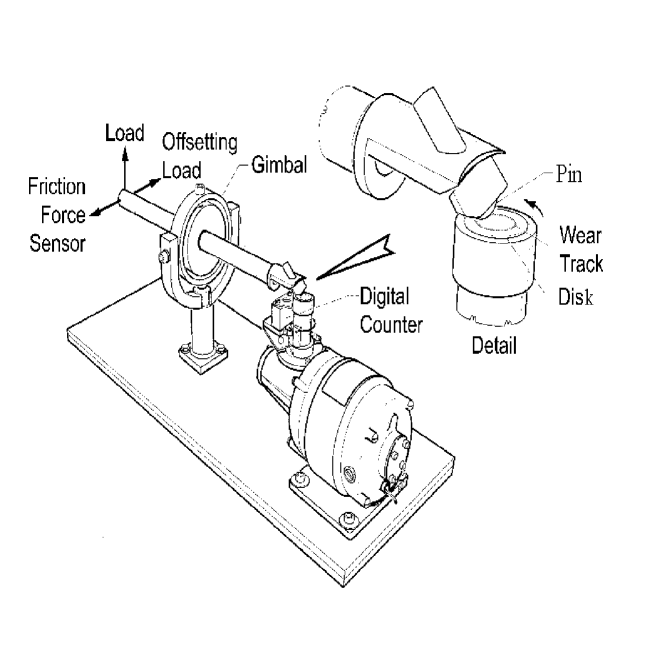
Figure 1: Pin-on-disk tribometer. The arrow points at the location where the spherical pin and the disk touch. The disk lies horizontally while the pin attached to the arm, rests above it.

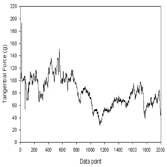
Figure 2: Typical signal from the tribometer. The effective spring constant of the apparatus is $~{}1$g/${\mu}$m, giving the largest force jumps as a few hundred ${\mu}m$.

The pin-on-disk tribometer used for these experiments is shown in Fig. 1. This configuration was chosen because it allows for easy replacement of the contacting surfaces, and it is the standard method for measuring friction and wear in unlubricated and lubricated contacts. The apparatus uses a $2.54$ cm diameter disk and a spherical pin with a $0.95$ cm radius machined on its end. The pin is attached to a load arm that is mounted on a gimbal supported at the center through which a load applied at the end of the arm is transferred to the contact zone. A strain-gauge is mounted at the end of the arm to monitor tangential friction force. The tangential force is monitored at a sample rate of 1,000 scans/sec and conversion is done using a 16-bit data acquisition card controlled by LabVIEW. Data is recorded to a text file for later analysis. Frictional force measurements are done on matching aluminum and steel (M50) pin-and-disc tribometers. The signal is collected at 1KHz during 16min, thus collecting $10^{6}$ points. The first quarter of each data set, or about 4 minutes, is discarded to assure that steady state is reached. In order to drive the system very slowly away from static equilibrium, we select slow rotational speeds in the range 10-20 RPM. Each disk is used for up to four tests by changing the radial position of the pin on the disk. Loads for aluminum range from 250 g to 1000 g. Steel is studied with a 1000 g normal load between pin and disk. Figure 2 shows a typical tangential friction force time series. It shows force jumps of various sizes. We first construct the probability distribution of force jumps. Force jumps are taken as those events corresponding to negative changes in the tangential force.

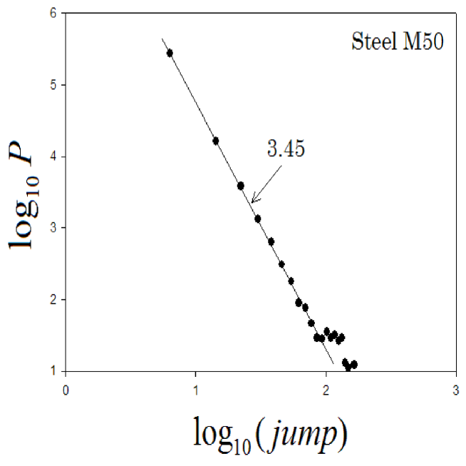
Figure 3: Probability density for jump size distribution on steel M50.

We next obtain the probability distributions of the tangential friction forces corresponding to aluminum under various loads and M50 steel. Results of such analysis are presented in Figs. 3 through 6. We observe an approximate linear behavior on the double logarithmic plots suggesting the power law behavior of the distributions $P(F)\sim F^{\mu}$ with the exponents $\mu$ in the range between 2.2 and 5.4.

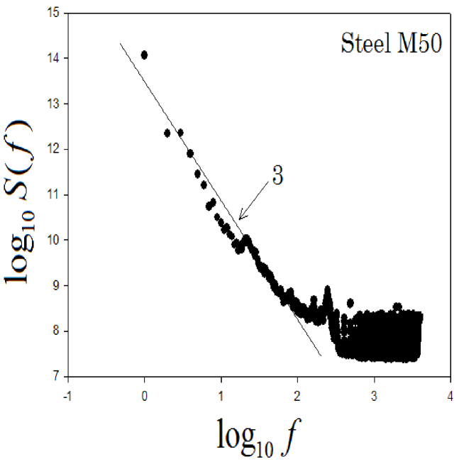
Figure 7: Power spectrum of jump sizes for a steel M50 sample.

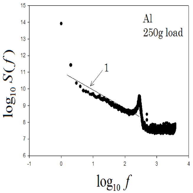
Figure 8: Power spectrum of jump sizes for an aluminum sample with a normal load of 250g.

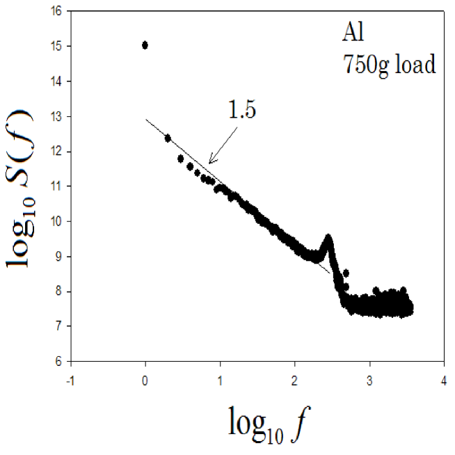
Figure 9: As in Fig. 8 with a normal load of 750g.

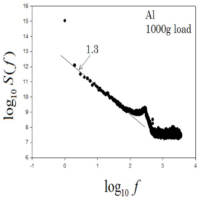
Figure 10: As in Fig. 8 with a normal load of 1000g.

We also compute the power spectra of the tangential friction force time series. We divide the original data ($2^{19}$) into $2^{8}$ statistically independent non-overlapping data sets of $2^{11}$ points each. Next, we calculate $2^{8}$ individual power spectra and finally average them to obtain the resulting power spectrum. Specific double-logarithmic plots are shown in Figs. 7-10. The power spectra follow power laws with exponents $1.0\leq\alpha\leq 2.6$. The results of the probability distribution and power spectra analysis are summarized in Table I.

III Theory

Friction is believed to occur on the atomic scale due to asperities on the surfaces in contacts. The simplest way to model such asperities is to use lattice models in the spirit of the invasion percolation Guyon , the sandpile model Bak , Bak-Sneppen evolution model Sneppen , and Zaitsev’s Robin Hood model Zaitsev . In general, these models are too crude to provide quantitative agreement with all experimental statistical quantities. However, quantities such as distribution of avalanche sizes are usually described by power laws characterized by exponents belonging to a few distinct universality classes. These exponents may be compared with experimentally found ones. If several models belong to the same universality class, it is reasonable to study the simplest among them, since it will provide the clearest understanding of the physical mechanisms of the phenomenon under study. One such simple and elegant example is the Robin Hood model, which was originally proposed for dislocation movement Zaitsev and later was adopted for modeling dry friction Slanina by Slanina who added to the original Robin-Hood model several parameters aimed to better capture the dry friction mechanism, but essentially obtained the same type of behavior as the original model had. Here we return to the original Robin Hood model due to its simplicity.

The model consist of a $d$-dimensional lattice. Each site $i$ on this lattice at any time step $n$ is characterized by the height $h_{i}(n)$ which we assume to be the height of an atomic scale asperity at a given point of the interface between two bodies in contact. Here we present the model for $d=1$, which is an appropriate choice to model slide friction but the analytical treatment is the same in any dimension, although the physically relevant cases are only $d=1$ and $d=2$. As the bodies slide against each other, the asperity with the maximal height is destroyed and some random number of atoms from this asperity is distributed among the neighboring asperities. To be specific, at each time step the site $i$ with maximal height $h_{m}(n)=\max h_{i}(n)$ is found and the new heights are determined according to the following rule: $h_{m}(n+1)=h_{m}(n)-r(n)$ and $h_{m\pm 1}(n+1)=h_{m\pm 1}(n)+r(n)/2$, where $r(n)$ are independent random variables uniformly distributed between 0 and 1. (Robin Hood determines the richest merchant in the market, robs him by a random amount $r(n)$ and distributes it equally among the neighbors without leaving anything for himself). If we assume periodic boundary conditions so that the sites with $i=0$ and $i=L$ are equivalent, the total amount of matter $\sum_{i=0}^{L}h_{i}(n)$ is conserved and we can assume it to be zero. The distance between the surfaces at a given site $i$ can be determined as $h_{m}(n)-h_{i}(n)$.

The particular details of the model such as the distribution of $r(n)$ or the rule of dividing it among neighbors can vary, but the model still retains its SOC behavior . The critical exponents appear to be sensitive to the details of dividing $r(n)$, for example, an exactly solvable asymmetric model (in which all the profit is given to the site on the left) Maslov95 belongs to a different universality class.

It has been shownMaslov ; Paczuski that in a wide class of depinning SOC models, all the critical exponents can be expressed in terms of the two main exponents : avalanche dimension $D$ and correlation exponent $\nu$. The avalanche of threshold $h_{0}$ is defined as sequence of time steps during which the hight of the maximal asperity is above $h_{0}$. Namely, if $h_{m}(n_{0})\geq h_{0}$ and $h_{m}(n_{0}+s)\geq h_{0}$ while for $n_{0}<n<n_{0}+s$, $h_{m}(n)<h_{0}$, the sequence $n=n_{0}+1,..,n_{0}+s$ is called a punctuating avalanche of threshold $h_{0}$ and mass $s$. The avalanche dimension describes how the avalanche mass $s$, scales with the horizontal dimension of the avalanche $R$. To be more precise, the mass distribution of forward avalanches with threshold $h_{0}$, scales as

$$P_{s}(s)\sim s^{-\tau_{s}}g_{s}(s(h_{0}-h_{c})^{D\nu})$$ (1)

and the distribution of the avalanche horizontal size, $R$, scales as

$$P_{R}(R)\sim R^{-\tau_{R}}g_{R}(R(h_{0}-h_{c})^{\nu}),$$ (2)

where $h_{c}\approx 0.114$ is the critical height,

$$\tau_{s}=1+(d-1/\nu)/D$$ (3)

and

$$\tau_{R}=1+d-1/\nu$$ (4)

are Fisher exponents first introduced to characterized cluster distributions in percolation theory Stauffer , while $g_{s}$ and $g_{R}$ are exponentially decreasing cutoff functions. It has been suggested Roux , that the Robin Hood model belongs to the same universality class as the linear interface model, for which the values ($D=2.23$ and $\tau_{s}=1.13$ in $d=1$; $D=2.725$ and $\tau_{s}=1.29$ in $d=2$) are given in Ref.Paczuski . Using these values and Eq. (3), one gets $\nu=1.41$ for $d=1$ and $\nu=0.83$ for $d=2$.

It can be shown that after the initial equilibration number of time steps $T\sim L^{D}$, any initial shape of the interface $h_{i}(0)$ reaches a steady state such that very few $N(L)$ “rich” sites have $h_{i}(n)>h_{c}\approx 0.114$, where

$$N(L)\sim L^{d_{f}}$$ (5)

and

$$d_{f}=d-1/\nu$$ (6)

plays the role of fractal dimension of rich sites. Only those few rich sites have a chance to be robbed. The chance $P_{m}(h_{m})$ that at a given time step, the maximal height is equal to $h_{m}$ decreases for an infinite system Maslov as

$$P_{m}(h_{m})=(h_{m}-h_{c})^{\gamma-1},$$ (7)

where the exponent

$$\gamma=1+\nu(D-d)$$ (8)

characterizes the dependence of the average avalanche size on its threshold $h_{0}$: $\langle s\rangle\sim(h_{0}-h_{c})^{-\gamma}$.

The distribution of heights of the poor sites converges to a smooth distribution on the interval $[h_{c}-1,h_{c}]$, while the distribution of the rich sites converges to the distribution with a power law singularity

$$P_{h}(h)\sim(h-h_{c})^{-d\nu}.$$ (9)

This result is not presented in Refs. Maslov ; Paczuski but can be justified by the following heuristic arguments. Indeed, the number of sites with $h>h_{0}$ scales as the number of the active sites in an avalanche of threshold $h_{0}$, and thus scales as $R^{d_{f}}(h_{0})$, where $R(h_{0})$ is the cutoff of the avalanche distribution (2) which scales as

$$R(h_{0})\sim(h_{0}-h_{c})^{-\nu}.$$ (10)

Thus the probability that $h>h_{0}$ scales as $(h_{0}-h_{c})^{-d_{f}\nu}$ and the probability density of $h=h_{0}$ scales as

$$P_{h}(h_{0})\sim(h_{0}-h_{c})^{-d_{f}\nu-1}=(h_{0}-h_{c})^{-d\nu}.$$ (11)

We can assume that the friction force, $F(n)$, at a given time step is proportional to the number $P_{h}(h_{m}(n))\Delta h$ of asperities with heights between $h_{m}(n)-\Delta h$ and $h_{m}(n)$:

$$F(n)=F_{1}P_{h}(h_{m}(n))\Delta h,$$ (12)

where $\Delta h$ is the interaction distance of atomic forces acting between the two surfaces and $F_{1}$ is a proportionality coefficient, corresponding to the surfaces interaction force at the asperity. Accordingly, the distribution of the friction forces $P(F)$ satisfies the equation $P(F)dF=P_{m}(h_{m})dh_{m}$, where the random variables $F$ and $h_{m}$ are linked by Eq. (12). Taking into account Eqs. (9) and (12) we have $dh_{m}/dF\sim dF^{-1/d\nu}/dF\sim F^{-1/d\nu-1}$. Finally Eq. (7) yields

$$P(F)=P_{m}(h_{m}(F)){dh_{m}\over dF}\sim F^{-(\gamma-1)/d\nu}F^{-1/d\nu-1}=F^{-\mu},$$ (13)

where

$$\mu=(D+1/\nu)/d.$$ (14)

For $d=1$, using values of Ref.Paczuski we have $P(F)=F^{\mu}$ with $\mu=2.94$ which is consistent with the experimental observations of the density of jump sizes presented here and in Ref.Zypman . For $d=2$ we have $\mu=1.96$.

In order to test this theoretical predictions, we perform simulations of the one dimensional Robin Hood model. Starting at $n=0$ with a flat interface $h_{i}(0)=0$, and selecting the first site to rob at random, after $T$ steps we get all $L$ sites of the interface updated at least once. Measuring the average $\langle T\rangle$ for many independent runs for different system sizes, and plotting it versus $L$ in a double-logarithmic scale (Fig. 11), we can obtain the avalanche dimension $D$ as the limit of the successive slopes of this graph for $L\to\infty$.

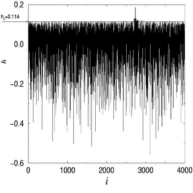
Figure 12: A typical shape of the steady state interface. The horizontal line shows the critical height.

A typical shape of the interface at time $n>T$ is presented in Fig. 12. One can see that the height of the majority of sites do not exceed the critical value $h_{c}\approx 0.114$. Interestingly, the majority of rich sites with heights above the critical barrier are localized in the vicinity of the richest site.

Figure 13 shows the histogram of all the interface heights $P_{h}(h)$ collected over many time steps after the system has reached the steady state and the histogram of the heights of the robbed sites $P_{m}(h_{m})$. One can see that while $P_{h}(h)$ dramatically increases as $h\to h_{c}^{+}$, no sites below the critical value are robbed and $P_{m}(h_{m})\to 0$ as $h_{m}\to h_{c}^{+}$. In order to find the exponents governing the behavior of these distributions near the critical point, we plot these quantities in a double logarithmic scale as functions of $h-h_{c}$ (Fig. 13b).

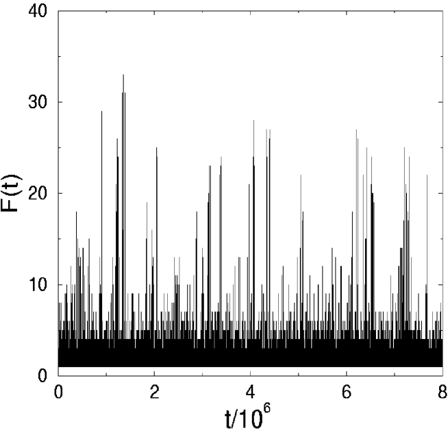
Figure 14: Time series of $F(t)$ for L=4096, $\Delta h=2^{-10}$

Finally we determine the time series of forces, defined as the number of heights between $h_{m}(n)$ and $h_{m}(n)-\Delta h$ as function of time. (Fig. 14). The histogram of this time series is presented in Fig. 15 in a double logarithmic scale. The slope of this plot is $\mu=3.0$, which is consistent with the theoretical prediction (14).

Note that the time series $F(n)$ is slightly correlated, which can be demonstrated by the negative slope of its power spectrum $S_{F}(f)\sim f^{-\alpha}$ in the log-log scale (Fig.16). The explanation of this phenomenon is based on the fact that values $h_{m}(n)$ fluctuate in the vicinity of $h_{c}$ in a non-trivial way, so that $h_{m}(n)$ become less than $h_{c}+\epsilon$ at time steps $n$ separated by intervals distributed according to Eq. (1). This is because these intervals coincide with avalanches for the threshold $h_{0}=h_{c}+\epsilon$. The values of $h_{m}(n)$ below $h_{c}+\epsilon$ correspond to the large values forces $F(n)$ and thus the intervals between the forces $F(n)$ above certain threshold are also distributed according to Eq. (1). It can be shown Paczuski ; Lowen that the exponent $\alpha$ of a time series generated by peaks separated by intervals of zero signal distributed according to a power law as in Eq. (1) is equal to $\tau_{s}-1$ for $1<\tau_{s}<2$. Thus according to Eq. (3) $\alpha=(d-1/\nu)/D\approx 0.13$. Indeed, the numerical data of Fig. 16 give $\alpha\approx 0.14$ in a very good agreement to the above theoretical prediction. However, this value of spectral exponent is much smaller than the values observed experimentally which are in the range between 1 and 2.6.

This difference is to be expected since the materials in contact as well as the strain gauge have finite elastic constants and inertia which produce a time delay between the applied force and the displacement record by the tribometer and lead to an effective integration of the input force time series. We would expect that if the materials were infinitely stiff then the experimental force power spectrum should agree with the theoretical predictions. Therefore, we construct a mechanical model of a tribometer, that accounts for these effects.

We assume that the pin of the tribometer contacts the sample at time $t$ at a point with coordinate $x(t)$ and it is dragged along the sample by the strain gauge spring with spring constant $k$ attached to the body of the instrument moving along the sample with constant velocity $v_{0}$, which is equivalent to the rotational speed of the disk. The force measured by the tribometer is thus $k[v_{0}t-x(t)]$, which fluctuates as the pin moves against the sample with velocity $v(t)=dx/dt$ and acceleration $a(t)=d^{2}x/dt^{2}$. The equation of motion of the pin is thus

$$ma=(v_{0}t-x)k-F(t,v),$$ (15)

where $F(t,v)$ is the friction force generated by the highest asperity of the sample and $m$ is the mass of the pin.

Now our goal is to relate $F(t,v$) with the input from the Robin Hood model. Note, that the physical time $t$ is not directly proportional to the time step $n$ of the Robin Hood model, but is equal to the sum of the durations of each time step

$$t=\sum_{i=1}^{n}t_{i},$$ (16)

where the durations $t_{i}$ are the times needed for the pin to travel a characteristic distance $\Delta x$, which is the linear size of each asperity. We assume that if the pin moves along the sample by $\Delta x$ , the current asperity is destroyed and the landscape of the contact between the pin and the sample is rearranged according to the rules of the model. Thus the time step $n_{t}$ of the Robin Hood model, corresponding to a given moment of time $t$ can be determined as $n_{t}={\rm int}[x(t)/\Delta x]$, where ${\rm int}[...]$ denotes the integer part of the expression in the brackets.

If $v=0$, $F(t,v)={\rm sign}(v_{0}t-x)\min[bF(n_{t}),k(v_{0}t-x)]$, where $F(n_{t})$ is the input from the Robin Hood model, and $b$ is some material and load-dependent constant. If $v\neq 0$, $F(x,v)={\rm sign}(v)[bF(n_{t})+\eta v]$, where $\eta>0$ is some dissipative constant. Constant $b$ is proportional to the load and depends on the elastic properties of the material. Introducing dimensionless variables by $x^{\prime}=x/\Delta x$ and $t^{\prime}=tv_{0}/\Delta x$, we arrive to a dimensionless equation

$$a^{\prime}=(t^{\prime}-x^{\prime})k^{\prime}-F^{\prime}(t^{\prime},v^{\prime}),$$ (17)

where $k^{\prime}=k\Delta x^{2}/mv_{0}^{2}$ and $F^{\prime}(t^{\prime},v^{\prime})$ is the same as $F(t,v)$ but the constants $b$ and $\eta$ are changed by $b^{\prime}=b\Delta x/mv_{0}^{2}$, $\eta^{\prime}=\eta\Delta x/mv_{0}$.

Thus, there are three independent dimensionless parameters of the model: $k^{\prime}$, $b^{\prime}$ and $\eta^{\prime}$. Varying these parameters, we found a wide region in the parameter space in which the power spectrum of the model resembles the experimental one. A typical example of the spectrum for $k^{\prime}=0.001$, $b^{\prime}=0.3$ and $\eta^{\prime}=0.01$ is shown on Fig.(17). The frequency of the resonance peak is determined by $\sqrt{k^{\prime}}/2\pi\approx 5\cdot 10^{-3}$. The peak becomes more pronounced as we decrease $\eta^{\prime}$. The increase in $\eta^{\prime}$ also increases the slope of the spectrum. The increase of $b^{\prime}$ at given $k^{\prime}$ increases the frequency region in which the power spectrum follows the power law but it also increases the absolute value of the slope closer to $2$, a characteristic value of the Brownian motion. In general, an integration of the time series corresponds to the increase of the spectral exponent by 2, so the integration of the white noise produces the Brownian noise. The observed spectral exponent $\alpha=1.45$ suggests that in a certain range of parameters, our model acts as the fractional integrator of the input signal. For a very stiff spring and large dissipation ($k=1$, $b=0.1$, $\eta=1$) the output signal of our equation is not much different from the input time series $F(n_{t})$ and we recover the small value of the spectral exponent $\alpha=0.14$.

IV Conclusions

We present experimental results and theoretical arguments that support the presence of self organized criticality in dry sliding friction. The experiments are pin-on-disk friction force traces of aluminum-aluminum and steel-steel systems. In both cases and for a variety of normal loads, the distribution of the friction force jumps and the frequency power spectra are power laws. The theoretical arguments are based on the application of the Robin Hood model to the friction problem. This model provides rules by which the surface profile changes as a function of time. The model introduces a height $h$ that we interpret physically as the height of the asperity. At each time step, atoms from the highest asperity are distributed among neighboring sites. We use the known distribution of heights and of maximal heights $h_{m}$ of the Robin Hood model to obtain the time series of the friction forces created by the asperities. As the maximum height fluctuates near the critical value, the number of smaller asperities whose heights are within the reach of atomic forces also fluctuates, diverging as $h_{m}$ comes close to the critical value $h_{c}$. These smaller asperities correspond to the contact sites and are responsible for the friction force. Specifically, the friction force is proportional to the number of contacts. Thus we propose that the friction force at a given time step is proportional to the probability density of the interface heights at the current value of the maximal height. The statistical distribution of the friction forces is studied both numerically and analytically.

We also find that the large forces are bunched in time. This is due to fluctuations of the maximal heights above a constant critical height. When the maximum heights return to the critical value, the forces become large. Thus, the surface waxes and wanes between a situation of large force due to many asperities acting, and a situation of smaller force in which only few asperities are in contact.

In addition, we use the time series of forces as an input to the Newton’s equation which describes the kinematics of the pin. For stiff or massless materials, the experimental distribution of force jumps should coincide with the theoretical distribution of forces. However, materials have finite mass and elasticity and thus the experimentally measured friction forces differ from the actual forces at the contact. To investigate these effects, we solve this equation numerically for different values of the parameters and find good agreement with the experiment.

V Acknowledgments

.

SVB thanks Yeshiva University for providing the high performance computer cluster that made this work possible. FRZ acknowledges support by Research Corporation through grant CC5786. FRZ thanks Phillip Abel, Mark Jansen, Kathleen Scanlon of NASA-Glenn Tribology Group for collaboration in the initial stages of this project.

Table 1: The values of exponents $\mu$ characterizing the power law behavior of the distribution of the force jump sizes and spectral exponents $\alpha$ characterizing the power spectrum of the friction force time series for different materials and loads.

Material	Load	$\mu$	$\alpha$
M50	1000g.	3.5	3.0
Al	250g.	5.4	1.0
Al	750g.	2.2	1.5
Al	1000g.	3.2	1.3

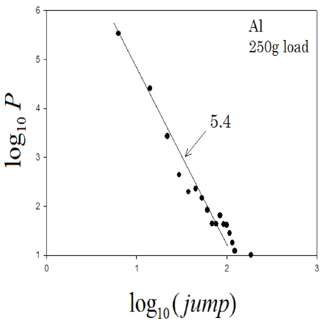
Figure 4: Probability density for jump size distribution on aluminum with a normal load of 250g.

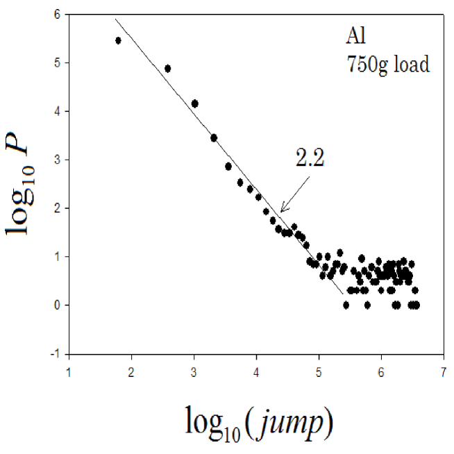
Figure 5: As in Fig. 4 with normal load of 750g.

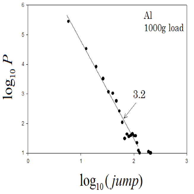
Figure 6: As in Fig. 4 with normal load of 1000g.

Figure 11: Double logarithmic plot of the average equilibration time $\langle T\rangle$ versus system size $L=2^{3},2^{4},...,2^{12}$. The inset shows the successive slopes of the main graph versus $1/L$. The intercept $D=2.23$, agrees with the data of Ref.Paczuski .

Figure 13: (a) The semi-logarithmic plot of the distribution of heights $P_{h}(h)$ of all sites (solid line) and the distribution of heights $P_{m}(h_{m})$ of robbed sites (dashed bold line). Vertical dotted line shows the position of the critical height $h_{c}=0.114$. (b) Double logarithmic plot of the same quantities plotted as functions of $h-h_{c}$. The slopes of the curves in the fitted regions are in agreement with Eq.(9) $-d\nu=-1.4$ and Eq. (7) $\nu(D-1)=1.72$.

Figure 15: Distribution of forces $P_{F}(F)$ for L=8192, $\Delta h=2^{-10}$. The slope of the straight line fit is $-\mu=-3$.

Figure 16: Power spectrum of the time series F(t) presented in Fig.(14). The slope of the straight line fit is $-\alpha-0.14$.

Figure 17: Power spectrum of the time series produced by Eq.(17) for $k^{\prime}=0.001$, $b^{\prime}=0.3$ end $\eta^{\prime}=0.01$.

References

- (1) R. Hallgass, V. Loreto, O. Mazzella, G. Paladin, L. Pietronero, Phys. Rev. E 56, 1346 (1997).
- (2) F.-J. Elmer, Phys. Rev. E 56, R6225 (1997).
- (3) R.V. Sole, S. C. Manrubia, Phys. Rev. E 54, R42 (1996).
- (4) V. Plerou, P. Gopikrishnan, L.A. Nunes Amaral, M. Meyer, and H.E. Stanley, Phys. Rev. E 60 6519 (1999).
- (5) O. Peters, C. Hertlein, K. Christensen, Phys. Rev. Lett. 88, 018701-1 (2002).
- (6) F. Slanina, Phys. Rev. E 59, 3947 (1999).
- (7) S. Ciliberto, C. Laroche, J. Phys. I France 4, 223 (1994)
- (8) D.P. Vallette, J.P. Gollub, Phys. Rev. E 47, 820 (1993)
- (9) P. Bak, C. Tang, and K. Wiesenfeld, Phys. Rev. Lett. 59 381 (1987).
- (10) H. J. Jensen , Self-Organized Criticality: Emergent Complex Behavior in Physical and Biological Systems, Cambridge Lecture Notes in Physics (No. 10) (London, 1998).
- (11) D.L. Turcotte, Rep. Prog. Phys. 62, 1377 (1999).
- (12) S. I. Zaitsev, Physica A 189 411 (1992).
- (13) S. Raux and E. Guyon, J. Phys. A 22 3693 (1989)
- (14) P. Bak and K. Sneppen, Phys. Rev. Lett. 71, 4083 (1993)
- (15) S. Maslov and Y.-C. Zhang, Phys. Rev. Lett. 75 1550 (1995)
- (16) S. Maslov, Phys. Rev. Lett. 74 562 (1995)
- (17) M. Paczuski, S. Maslov, and P. Bak , Phys. Rev. E 53 414 (1996).
- (18) D. Stauffer and A. Aharony, Introduction to Percolation Theory (Taylor & Francis, Philadelphia, 1994).
- (19) S. Raux and A. Hansen, J. Physique I 4 515 (1994)
- (20) F. R. Zypman,J. Ferrante, M. Jansen, K. Scanlon, and P. Abel, J. Phys.-Cond. Mat.15 L191 (2003)
- (21) S. B. Lowen and M. C. Teich, Phys. Rev. E, 47, 992 (1993).