Coupled-channel pseudo-potential description of the Feshbach resonance in two dimensions

Abstract

We derive pseudo-potentials that describe the scattering between two particles in two spatial dimensions for any partial wave $m$, whose scattering strength is parameterized in terms of the phase shift $\delta_{m}$. Using our $m=0$ pseudo-potential, we develop a coupled channel model with 2D zero-range interactions, which describes the two-body physics across a Feshbach resonance. Our model predicts the scattering length, the binding energy and the “closed channel molecular fraction” of two particles; these observables can be measured in experiments on ultracold quasi-2D atomic Bose and Fermi gases with present-day technology.

The success in creating Bose-Einstein condensates and Fermi degenerate gases has resulted in a renewed interest in the scattering between two atoms. At very low temperatures the de Broglie wavelengths of the atoms are large compared to the typical Van der Waals length of atom-atom potentials. As a result, atoms at ultracold temperatures do not probe the detailed structure of the interaction potential. Consequently, the shape-dependent potential can be replaced by an appropriate zero-range (ZR) pseudo-potential, which is characterized by a single parameter, the generalized scattering length. For example, $s$-wave scattering in three spatial dimensions can in many cases be described accurately through Fermi-Huang’s pseudo-potential huan57 . Generalizations of Fermi-Huang’s pseudo-potential, applicable to higher partial wave scattering in 3D, have also been considered huan57 ; kanj04 ; stoc05 . The foremost advantage of using ZR pseudo-potentials is that a number of two-body and some many-body problems become analytically solvable, thus highlighting the physical meaning of a few key parameters.

An exciting development in the area of ultracold atom physics is the creation of low-dimensional quantum gases. The trapping of bosons in quasi-1D geometries, e.g., has allowed the fermionization of 1D Bose gases to be verified experimentally bloch04 and the binding energy of 1D molecules to be extracted from experiment mori05 . This paper considers quasi-2D systems, for which the motion in the tight confining direction, the $z$-direction, is frozen out petr00 ; grimm . The equation of state then depends on the (generalized) 2D scattering length. A thorough understanding of the two-particle physics in 2D for any partial wave would aid studies of the 2D many-body problem. Toward this end, we derive 2D ZR pseudo-potentials for any partial wave $m$ and develop a coupled channel model applicable to two particles with $m=0$ across a Feshbach resonance.

Experiments on ultracold gases routinely utilize Feshbach resonances, which allow the interaction strength between two particles to be tuned to essentially any value through application of an external magnetic field. A detailed understanding of Feshbach resonances in 3D underlies studies of, e.g., the BEC-BCS crossover and $p$-wave pairing. Confinement induced resonances in 2D have been predicted petr00 ; italian , and recently been observed for $p$-wave interactions gunter , thus allowing the effective 2D coupling constant to be tuned to essentially any value including zero and infinity. Assuming a strictly 2D geometry, we propose a coupled channel model for the lowest partial wave, i.e., $m=0$, with four parameters, the scattering lengths $b_{1}$ and $b_{2}$ of the “open” and “closed” channel, the coupling strength $\beta$ and the detuning $\epsilon$. While $b_{1}$, $b_{2}$ and $\beta$ are fixed for a given system, varying the detuning $\epsilon$ corresponds to changing the strength of an external magnetic field. To the best of our knowledge, no coupled-channel model for 2D resonances has been proposed to date. Our model predicts that the dependence of the effective 2D scattering length on the external control parameter is distinctly different than that of the effective 3D scattering length, thus highlighting the non-intuitive behavior of systems with reduced dimensionality. We also determine the binding energy and the occupation of the open and closed channel across a 2D resonance. These observables have been measured across a 3D resonance observable_experiment1 ; observable_experiment2 but not yet across a 2D resonance; however, we expect measurements on quasi-2D systems to be performed in the near future.

To derive 2D ZR potentials for any partial wave we assume that the atom-atom potential $V_{int}(\rho)$ depends only on the distance $\rho$ between the two atoms, that is, we neglect any angular dependence that may arise from spin-dependent interactions. The center of mass motion can then be separated off, and the radial Schrödinger equation reads

$$\left[\frac{\partial^{2}}{\partial\rho^{2}}+\frac{1}{\rho}\frac{\partial}{\partial\rho}-\frac{m^{2}}{\rho^{2}}-\frac{2\mu}{\hbar^{2}}\left(V(\rho)-E\right)\right]R_{m}(\rho)=0,$$ (1)

where $\mu$ denotes the reduced mass of the two-atom system, and $V(\rho)=V_{int}(\rho)+V_{ext}(\rho)$ [$V_{ext}(\rho)$ denotes the $\rho$-dependent part of an external confining potential, see below; for now we set $V_{ext}=0$]. In Eq. (1), $m$ denotes the orbital quantum number; $m=0$ applies to scattering between two 2D bosons or two 2D fermions with opposite spin, $m=1$ to scattering between two spin-polarized fermions, and so on. We now derive $m$-dependent 2D ZR pseudo-potentials, $V_{int}(\rho)=V^{ps}_{m}(\rho)$, which reproduce the low-energy observables of a shape-dependent short-range atom-atom potential.

We write the pseudo-potential $V^{ps}_{m}(\rho)$ in terms of a $\delta$-shell of radius $s$ and a yet to be determined operator $\hat{O}_{m}(\rho)$ stoc05 ,

$$V^{ps}_{m}(\rho)={\{\hat{O}_{m}(\rho)\delta(\rho-s)\}}_{s\rightarrow 0}.$$ (2)

The solutions to Eq. (1) for $V_{int}=V_{m}^{ps}$ can be written in terms of the cylindrical Bessel functions $J_{m}(k\rho)$ and $N_{m}(k\rho)$. For $\rho<s$, only $J_{m}$, which is regular at the origin, contributes,

$$R^{-}_{m}(\rho)=B_{m}J_{m}(k\rho),$$ (3)

where $k=\sqrt{2\mu E/\hbar^{2}}$. The $\delta$-shell introduces a phase shift $\delta_{m}(k)$ of the $m$th partial wave so that the wave function for $\rho>s$ is given by

$$R^{+}_{m}(\rho)=A_{m}\left[J_{m}(k\rho)-\tan(\delta_{m}(k))N_{m}(k\rho)\right].$$ (4)

In Eqs. (3) and (4), $B_{m}$ and $A_{m}$ denote constants to be determined below.

For $s$-wave scattering ($m=0$), the phase shift $\delta_{0}(k)$ determines the 2D energy-dependent scattering length $a_{0}(k)$ verhaar ,

$$a_{0}(k)=\frac{2}{k}\exp\left[\frac{\pi}{2}\cot\delta_{0}(k)-\gamma\right],$$ (5)

where $\gamma$ denotes Euler’s constant. The energy-dependent scattering length $a_{0}(k)$, which is always greater or equal to zero, is defined such that the scattering wave function has a node at $\rho=a_{0}(k)$. The unusual functional form of $a_{0}(k)$, i.e., the exponential dependence on the phase shift, is a direct consequence of the logarithmic dependence of $N_{m}(k\rho)$ on $k\rho$, $N_{0}(k\rho)\approx\frac{2}{\pi}[\ln(k\rho/2)+\gamma]$ for $k\rho\rightarrow 0$. For higher partial waves, we define generalized energy-dependent “scattering lengths” $a_{m}(k)$, which have dimensions of (length)^2m, as

$$a_{m}(k)=-\frac{\tan(\delta_{m}(k))}{k^{2m}}\frac{\Gamma(m)\Gamma(m+1)2^{2m}}{\pi}.$$ (6)

Since $a_{1}(k)$ has dimensions of (length)² we refer to it as scattering area. Energy-independent generalized scattering lengths $a_{m}$ are readily defined through $a_{m}=\lim_{k\rightarrow 0}a_{m}(k)$.

Imposing continuity of the wave function $R_{m}(\rho)$ at $\rho=s$, that is, requiring $R_{m}^{+}(s)=R_{m}^{-}(s)$, allows $B_{m}$ to be expressed in terms of $A_{m}$. Integrating the Schrödinger equation from $\rho=s-\epsilon$ to $s+\epsilon$, and then taking the limit $\epsilon\rightarrow 0$, results in

$$\frac{\hbar^{2}}{2\mu}\left[\frac{\partial}{\partial\rho}R^{+}_{m}(\rho)-\frac{\partial}{\partial\rho}R^{-}_{m}(\rho)\right]_{\rho=s}=\hat{O}_{m}(s)R_{m}(s).$$ (7)

Plugging Eqs. (3) and (4) into Eq. (7) and taking $ks\ll 1$, determines the operator $\hat{O}_{m}(s)$, and hence the pseudo-potential $V_{m}^{ps}(\rho)$. For $m=0$, we find

$$V_{0}^{ps}(\rho)=\left\{\frac{-\frac{\hbar^{2}}{\mu}\tan(\delta_{0}(k))}{\left(1-\frac{2\tan(\delta_{0}(k))}{\pi}f_{0}(k,\rho)\right)\pi\rho}\frac{\partial}{\partial\rho}\rho\delta(\rho-s)\right\}_{s\rightarrow 0},$$ (8)

where $f_{0}(k,\rho)=1+\gamma+\ln(k\rho/2)$. The explicit $k$ dependence of the $m=0$ ZR potential drops out when $V_{0}^{ps}$ is written in terms $a_{0}(k)$. Our $s$-wave pseudo-potential agrees with the $\Lambda$ potential derived in Ref. olsh02 if one sets $\Lambda$ equal to $k$ (see also Ref. wolsch ). Below, we use the boundary condition implied by the pseudo-potential $V_{0}^{ps}$ to develop a coupled-channel ZR model for 2D scattering.

For $m>0$, a straightforward yet somewhat tedious calculation gives

$$V_{m}^{ps}(\rho,k)=$$

$$\left\{\frac{-\frac{\hbar^{2}[\Gamma(m+1)]^{2}\tan(\delta_{m}(k))}{\mu(2m)!\pi}\left(\frac{2}{k}\right)^{2m}}{(1+\frac{\tan(\delta_{m}(k))}{\pi}f_{m}(k,\rho))\rho^{m+1}}\frac{\partial^{2m}}{\partial\rho^{2m}}\rho^{m}\delta(\rho-s)\right\}_{s\rightarrow 0},$$ (9)

where

$$f_{m}(k,\rho)=\bar{\psi}(m)-2\ln\left(\frac{k\rho}{2}\right)-\sum_{r=0}^{r=2m-1}\frac{2}{2m-r}.$$ (10)

Here, $\bar{\psi}(m)=\psi(1)+\psi(m+1)$, where $\psi$ denotes the digamma function. As written in Eq. (Coupled-channel pseudo-potential description of the Feshbach resonance in two dimensions), the $m>0$ pseudo-potential leads, despite the regularization operator, to divergencies at $\rho\rightarrow 0$ if the energy-dependent coefficients $C_{m}$ and $D_{m}$ of the $\rho^{-m}$ and $\ln(\rho)\rho^{m}$ terms in the expansion of the eigenfunction sought differ from the corresponding coefficients $c_{m}$ and $d_{m}$ of the expansion of the irregular free particle solution $N_{m}(k\rho)$. To cure this divergence, the right hand side of Eq. (Coupled-channel pseudo-potential description of the Feshbach resonance in two dimensions) has to be multiplied by $d_{m}C_{m}/(c_{m}D_{m})$, resulting in a pseudo-potential that has to be determined self-consistently tobepublished . A similar self-consistency condition is not needed for systems with odd dimensionality.

The bound state energies $E_{m}^{bind}$ of the pseudo-potentials $V_{m}^{ps}$ can be determined through analytic continuation stoc05 . For $m=0$, we recover the well known expression for the ZR binding energy $E_{0}^{bind}$ jens04 ,

$$E_{0}^{bind}=\frac{-\hbar^{2}}{2\mu(a_{0}(k))^{2}}\;4\exp(-2\gamma).$$ (11)

For $m>0$, the binding energies $E_{m}^{bind}$ are given by

$$E_{m}^{bind}=\frac{-2\hbar^{2}}{\mu[-i(-1)^{m}a_{m}(k)]^{1/m}}\;\left(\frac{\Gamma(m)\Gamma(m+1)}{\pi}\right)^{1/m}.$$ (12)

The occurance of an “$i$” in Eq. (12) appears odd at first sight. This puzzle is resolved by noting that the 2D generalized energy-dependent scattering lengths $a_{m}(k)$ with $m>0$ are, in contrast to the 1D and 3D counterparts, complex. Consequently, the binding energies $E_{m}^{bind}$ are determined by those $a_{m}(k)$ for which the real part vanishes. For $m=1$, e.g., we find excellent agreement between the exact binding energy determined from the energy-dependent scattering area via Eq. (12) and that for a square well potential with range $\rho_{0}$, $V_{int}(\rho)=V_{SW}(\rho)=-V_{0}$ for $\rho<\rho_{0}$ and zero otherwise.

We now use the proposed pseudo-potentials to determine the eigenspectrum of two atoms in 2D under external harmonic confinement, that is, in Eq. (1) we consider $V_{ext}(\rho)=\mu\omega^{2}\rho^{2}/2$. Such a two-body system can be realized experimentally with the aid of a 1D optical lattice with doubly-occupied lattice sites, for which the tunneling between neighboring sites is neglegible. The solutions for $\rho<s$ and $\rho>s$ are proportional to the confluent hypergeometric functions $M$ and $U$, i.e., $R_{m}^{-}(\rho)\propto\rho^{m}\exp(-\rho^{2}/2a_{ho}^{2})M(-\chi,m+1,\rho^{2}/a_{ho}^{2})$ and $R_{m}^{+}(\rho)\propto\rho^{m}\exp(-\rho^{2}/2a_{ho}^{2})U(-\chi,m+1,\rho^{2}/a_{ho}^{2})$, where $a_{ho}=\sqrt{\hbar/(\mu\omega)}$ denotes the oscillator length and $\chi$ a non-integer quantum number, $E_{m\chi}=(2\chi+1+m)\hbar\omega$. Enforcing continuity at $\rho=s$ determines the eigenenergies $E_{m\chi}$ implicitly in terms of $a_{m}(k)$,

$$(-1)^{m+1}\frac{\Gamma(-\chi-m)}{\Gamma(-\chi)}\sum_{r=0}^{m-1}\frac{(-\chi-m)_{r}(-1)^{m-r}}{(1-m)_{r}r!(2m-2r)!!}$$

$$=\frac{\ln\left(\chi+\frac{m+1}{2}\right)-\psi(-\chi)}{\Gamma(m)\Gamma(m+1)}+\frac{a_{ho}^{2m}}{a_{m}(k_{m\chi})}\frac{1}{\left(\chi+\frac{m+1}{2}\right)^{m}},$$ (13)

where $k_{m\chi}=\sqrt{2\mu E_{m\chi}}/\hbar$ and $(x)_{r}=x(x+1)\cdots(x+r-1)$ with $(x)_{0}=1$. Equation (Coupled-channel pseudo-potential description of the Feshbach resonance in two dimensions) contains the generalized energy-dependent blum02 2D scattering length $a_{m}(k)$ evaluated at $k=k_{m\chi}$ and is valid for $m>0$; for $m=0$ the eigenenergies are given by Eq. (Coupled-channel pseudo-potential description of the Feshbach resonance in two dimensions) with $\beta=0$ and $b_{1}=a_{0}(k)$.

Asterisks in Fig. 1 show the $m=1$ eigenenergies for two particles interacting through the proposed ZR potential, Eq. (Coupled-channel pseudo-potential description of the Feshbach resonance in two dimensions), under harmonic confinement over a large range of zero-energy scattering areas $a_{1}$. For comparison, solid lines show the exact eigenenergies, determined semi-analytically, for two particles under harmonic confinement interacting through a square well potential with range $\rho_{0}=0.01a_{ho}$. Figure 1 illustrates excellent agreement between the eigenenergies for two 2D particles interacting through the pseudo-potential and those interacting through the square well potential. We find similar behaviors for higher partial waves.

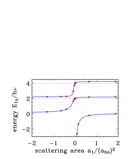
Figure 1: $E_{1\chi}$ as a function of $a_{1}(k=0)$ ($\omega=2\pi\nu$). Asterisks show $E_{1\chi}$, Eq. (Coupled-channel pseudo-potential description of the Feshbach resonance in two dimensions), for the energy-dependent pseudo-potential $V_{1}^{ps}(\rho)$ and solid lines show $E_{1\chi}$ for $V_{SW}$ with $\rho_{0}=0.01a_{ho}$. For comparison, horizontal dotted lines indicate the energy levels for $a_{1}=0$.

To describe the two-body physics across a 2D Feshbach resonance for two bosons or for two fermions with opposite spin, we develop a coupled-channel ZR model for $m=0$. For $\rho>0$, the wave function with components $R_{0}^{(1)}(\rho)$ and $R_{0}^{(2)}(\rho)$ satisfies the harmonic oscillator Schrödinger equation in the relative coordinate,

$$\left(\begin{array}[]{c}\left[\frac{\hbar^{2}}{2\mu}(\frac{\partial^{2}}{\partial\rho^{2}}+\frac{1}{\rho}\frac{\partial}{\partial\rho})-\frac{1}{2}\mu\omega^{2}\rho^{2}+E\right]R_{0}^{(1)}(\rho)\\ \left[\frac{\hbar^{2}}{2\mu}(\frac{\partial^{2}}{\partial\rho^{2}}+\frac{1}{\rho}\frac{\partial}{\partial\rho})-\frac{1}{2}\mu\omega^{2}\rho^{2}+E-\epsilon\right]R_{0}^{(2)}(\rho)\end{array}\right)=0,$$ (16)

where $\epsilon$ denotes a detuning ($\epsilon\geq 0)$, which can be changed, e.g., by varying the strength of an external magnetic field. The 2D pseudo-potential $V_{0}^{ps}$ imposes a boundary condition at $\rho=0$, which we parameterize as

$$\left(\begin{array}[]{cc}\ln(\rho/b_{1})&\beta\\ \beta&\ln(\rho/b_{2})\end{array}\right)\left(\begin{array}[]{c}\rho\frac{\partial}{\partial\rho}R_{0}^{(1)}\\ \rho\frac{\partial}{\partial\rho}R_{0}^{(2)}\end{array}\right)=\left(\begin{array}[]{c}R_{0}^{(1)}\\ R_{0}^{(2)}\end{array}\right).$$ (23)

The coupling between the two channels is characterized by the dimensionless parameter $\beta$. To ensure a divergence-free treatment, Eq. (23) takes this coupling parameter to be proportional to the derivative of the wave function components, and not, as done in 3D dunn05 , to be proportional to the wave function components themselves. The scattering length $a_{0}^{CC}(E,\epsilon)$ predicted by Eqs. (16) and (23) in the limit $\omega\rightarrow 0$ is

$$a_{0}^{CC}(E,\epsilon)=b_{1}\exp\left\{-\beta^{2}/\left[\gamma+\frac{1}{2}\ln\left(\frac{\mu b_{2}^{2}}{2\hbar^{2}}(\epsilon-E)\right)\right]\right\}.$$ (24)

To determine the behavior of the scattering length $a_{0}^{CC}(E,\epsilon)$ in the vicinity of the resonance as a function of the magnetic field strength $B$, we Taylor-expand $a_{0}^{CC}(E,\epsilon)$ about the resonance position $\epsilon_{R}$, which is given by the binding energy $E_{0}^{bind}$ of the strongly closed molecular channel, $\epsilon_{R}=2\exp(-2\gamma)\hbar^{2}/(\mu b_{2}^{2})$. We find a simple functional form for $a_{0}^{CC}(E=0,B)$ in terms of the background scattering length $A_{bg}$, the resonance width $\Delta$ and the resonance position $B_{R}$,

$$a_{0}^{CC}(E=0,B)=A_{bg}\exp[-\Delta/(B-B_{R})],$$ (25)

where $A_{bg}=b_{1}$, $B_{R}=\epsilon_{R}/M$ and $\Delta=2\beta^{2}\epsilon_{R}/M$ ($M$ denotes the difference in magnetic moment between atoms in the open and closed channel). Just as the 2D single-channel scattering length $a_{0}$ [Eq. (5)], the functional dependence of the 2D coupled-channel scattering length $a_{0}^{CC}$ on $B$ near a resonance is distinctly different from that of the 3D counterpart. In principle, the parameters $b_{1}$, $b_{2}$ and $\beta$ can be determined by comparing Eq. (25) with experimental data for a specific 2D Feshbach resonance. Since no such data exist to date, the inset of Fig. 2 illustrates the behavior of $a_{0}^{CC}$ as a function of $\epsilon$ for $E=0$, $a_{1}=0.5a_{ho}$, $a_{2}=0.05a_{ho}$ and $\beta=0.1$. The scattering length $a_{0}^{CC}$ changes from infinity to zero at the resonance value $\epsilon_{R}$ (indicated by a vertical dotted line).

We find an implicit eigenequation for the eigenenergies $E_{0n}$, $E_{0n}<\epsilon$, of the coupled-channel ZR model for two particles under harmonic confinement with $m=0$ [Eqs. (16) and (23)],

$$\beta^{2}\left\{\ln\left(\frac{b_{1}}{a_{ho}}\right)+\frac{1}{2}\psi\left(\frac{1}{2}-\frac{E_{0n}}{2\hbar\omega}\right)-\psi(1)\right\}^{-1}$$

$$=\left\{\ln\left(\frac{b_{2}}{a_{ho}}\right)+\frac{1}{2}\psi\left(\frac{1}{2}-\frac{E_{0n}-\epsilon}{2\hbar\omega}\right)-\psi(1)\right\}.$$ (26)

Figure 3 shows the eigenenergies $E_{0n}$ as a function of $\epsilon$ for $b_{1}=0.5a_{ho}$, $b_{2}=0.05a_{ho}$ and three different values of $\beta$, i.e., $\beta=0.03$ (solid lines), $0.1$ (dotted lines) and $\beta=0.3$ (dashed lines).

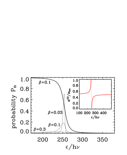
Figure 2: Molecular fractions $P_{0}$ (solid line) and $P_{1}$ (dotted lines), Eq. (27), for $b_{1}=0.5a_{ho}$, $b_{2}=0.05a_{ho}$ and different coupling constants $\beta$ as a function of $\epsilon$. Inset: 2D scattering length $a_{0}^{CC}(E,\epsilon)$ as a function of $\epsilon$ for $E=0$, $b_{1}=0.5a_{ho}$, $b_{2}=0.05a_{ho}$ and $\beta=0.1$.

The non-vanishing coupling leads to a series of energy level crossings at $\epsilon\approx\epsilon_{R}$, which become narrower as the coupling $\beta$ decreases. For higher-lying states, i.e., larger $E_{0n}$, the resonance of the energy-dependent scattering length $a_{0}^{CC}(\epsilon,E)$, Eq. (24), moves to larger $\epsilon$ values, and thus explains why the energy level crossings move to larger $\epsilon$ for higher $n$. The energy of the state $n=1$ for $\epsilon<\epsilon_{R}$ corresponds to the binding energy of the open channel, i.e., of channel $(1)$. We checked that a 2D coupled channel square-well system (see Ref. greene for the 3D analog) reproduces the results obtained for our proposed coupled-channel ZR system.

Our coupled channel model leads to a mixing of the strongly closed molecular channel $R_{0n}^{(2)}$ and the open channel $R_{0n}^{(1)}$. To quantify the admixture of the strongly closed molecular level across the resonance, we define the molecular fraction $P_{n}$ greene ,

$$P_{n}=\int|R_{0n}^{(2)}|^{2}\rho d\rho/\left[\int\left(|R_{0n}^{(1)}|^{2}+|R_{0n}^{(2)}|^{2}\right)\rho d\rho\right].$$ (27)

The main part of Fig. 2 shows $P_{n}$ for $b_{1}=0.5a_{ho}$, $b_{2}=0.05a_{ho}$ and different $\beta$ values as a function of $\epsilon$; a solid line shows $P_{0}$ for $\beta=0.1$, and dotted lines show $P_{1}$ for $\beta=0.03$, $0.1$ and $0.3$. The molecular fraction $P_{0}$ is close to one for small $\epsilon$, and drops to zero as $\epsilon$ is swept across the resonance. This indicates that the character of the $n=0$ state changes from “strongly closed molecular” to “weakly closed molecular” as $\epsilon$ changes from $\epsilon<\epsilon_{R}$ to $\epsilon>\epsilon_{R}$. The molecular fraction of the $n=1$ state is close to zero away from resonance for all coupling strengths considered. Near resonance, however, $P_{1}$ depends on $\beta$. For weak coupling, $P_{1}$ approaches one on resonance. For strong coupling, in contrast, $P_{1}$ is comparatively small as shown in Fig. 2 for $\beta=0.3$. This suggests that the 2D analog of the BEC-BCS crossover can be best studied utilizing 2D Feshbach resonances with strong coupling for which the admixture of the strongly closed molecular channel is small. Similar behavior is found for 3D systems moor05 .

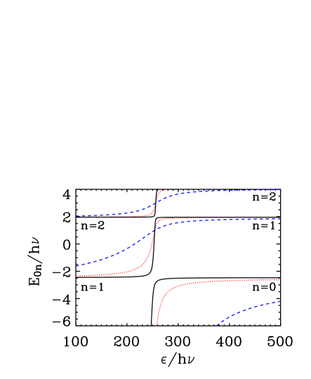
Figure 3: Eigenenergies $E_{0n}$, Eq. (Coupled-channel pseudo-potential description of the Feshbach resonance in two dimensions), for $b_{1}=0.5a_{ho}$, $b_{2}=0.05a_{ho}$ and three different values of $\beta$, i.e., $\beta=0.03$ (solid lines), $0.1$ (dotted lines) and $0.3$ (dashed lines) as a function of $\epsilon$.

In summary, this paper derives a series of 2D pseudo-potentials, which describe the low-energy scattering of two particles with partial wave $m$. The boundary condition implied by the $m=0$ pseudo-potential is then used to develop an analytically solvable coupled-channel model, which describes the physics across a 2D Feshbach resonance. The predicted dependence of the effective 2D scattering length $a_{0}^{CC}$ on the strength $B$ of the external magnetic field, Eq. (25), may prove useful in analyzing experimental data for quasi-2D Bose gases or two-component Fermi gases. We also determine the binding energy of 2D dimers, which can be measured with present-day technology by utilizing optical lattices with doubly-occupied lattice sites in the no-tunneling regime observable_experiment1 , across a Feshbach resonance.

Fruitful discussions with Chris Greene and Stefano Giorgini, and support by the NSF under grant PHY-0331529 are gratefully acknowledged.

References

- (1) K. Huang and C. N. Yang, Phys. Rev. 105, 767 (1957).
- (2) K. Kanjilal and D. Blume, Phys. Rev. A 70, 042709 (2004).
- (3) R. Stock, A. Silberfarb, E. L. Bolda and I. Deutsch, Phys. Rev. Lett. 94, 023202 (2005).
- (4) B. Paredes et al., Nature 429, 277 (2004); T. Kinoshita, T. Wenger and D. S. Weiss, Science 305, 1125 (2004).
- (5) H. Moritz et al., Phys. Rev. Lett. 94, 210401 (2005).
- (6) D. S. Petrov, M. Holzmann and G. V. Shlyapnikov, Phys. Rev. Lett. 84, 2551 (2000).
- (7) D. Rychtarik, B. Engeser, H.-C. Nägerl and R. Grimm, Phys. Rev. Lett. 92, 173003 (2004).
- (8) Z. Idziaszek and T. Calarco, Phys. Rev. Lett. 96, 013201 (2006).
- (9) K. Günter et al., Phys. Rev. Lett. 95, 230401 (2005).
- (10) T. Stöferle et al., cond-mat/0509211.
- (11) G. B. Partridge et al., Phys. Rev. Lett. 95, 020404 (2005).
- (12) B. J. Verhaar, J. P. H. W. van den Eijnde, M. A. J. Voermans and M. M. J. Schaffrath, J. Phys. A 17, 595 (1984).
- (13) M. Olshanii and L. Pricoupenko, Phys. Rev. Lett. 88, 010402 (2002).
- (14) K. Wódkiewicz, Phys. Rev. A 43, 68 (1991).
- (15) K. Kanjilal and D. Blume, to be published.
- (16) A. S. Jensen, K. Riisager, D. V. Fedorov and E. Garrido, Rev. Mod. Phys. 76, 215 (2004).
- (17) D. Blume and C. H. Greene, Phys. Rev. A 65, 043613 (2002); E. L. Bolda, E. Tiesinga and P. S. Julienne, idib. 66, 013403 (2002).
- (18) J. W. Dunn et al., Phys. Rev. A, 71, 033402 (2005).
- (19) M. G. Moore, cond-mat/0506383.
- (20) see http://lumberjack.colorado.edu/Feshbach/ (unpublished materials by C. H. Greene).