Generation of dynamic structures in nonequilibrium reactive bilayers

Abstract

We present a nonequlibrium approach for the study of a flexible bilayer whose two components induce distinct curvatures. In turn, the two components are interconverted by an externally promoted reaction. Phase separation of the two species in the surface results in the growth of domains characterized by different local composition and curvature modulations. This domain growth is limited by the effective mixing due to the interconversion reaction, leading to a finite characteristic domain size. In addition to these effects, first introduced in our earlier work [Phys. Rev. E 71, 051906 (2005)], the important new feature is the assumption that the reactive process actively affects the local curvature of the bilayer. Specifically, we suggest that a force energetically activated by external sources causes a modification of the shape of the membrane at the reaction site. Our results show the appearance of a rich and robust dynamical phenomenology that includes the generation of traveling and/or oscillatory patterns. Linear stability analysis, amplitude equations and numerical simulations of the model kinetic equations confirm the occurrence of these spatiotemporal behaviors in nonequilibrium reactive bilayers.

I Introduction

Due to hydrophobic repulsions, amphiphilic molecules such as lipids spontaneously aggregate in water to form bilayer membranes. These bilayers typically exhibit an in-plane fluidlike nature, and are highly flexible surfaces so they can display a large variety of conformations. The experimental study of equilibrium lipid bilayers has attracted a great deal of attention in the past decades lipnat ; lip . Issues such as membrane conformational behavior, shape fluctuations, fusion and fission, and phase segregation in multicomponent bilayers have been extensively investigated lipnat ; lip ; seif . Among many other manipulation techniques, the fabrication of synthetic giant vesicles and planar lipid membranes blm as well as micropipet aspiration evans have been used to perform these studies, leading to a fairly detailed current understanding of equilibrium membranes.

Parallel to the experimental advances, theoretical modeling of equilibrium flexible membranes has also come a long way. Typical theoretical approaches are based on the search for minimum energy conformations according to the Canham-Helfrich bending elasticity description canham ; nuovo of a tensionless membrane, plus (optionally) the corresponding area-difference contributions for closed surfaces adif . More recently, it has been recognized that internal degrees of freedom such as chemical composition can crucially influence the shape of the bilayer, especially when dealing with multicomponent membranes undergoing phase separation. In particular, models containing a local coupling between composition and curvature have been developed and ; sun ; goz ; dyn3 ; dyn2 ; dyn1 , resulting in an interesting outcome, namely, the appearance of phase separating domains that grow and adopt distinct membrane curvatures. This is understood as the initiation mechanism for budding phenomena in real membranes. Kinetic mesoscopic schemes, Monte Carlo approaches, and a variety of discrete dynamic algorithms have been proposed on this basis, and have mainly been devoted to the study of the equilibrium behavior and the dynamics toward equilibrium of flexible bilayers.

The ultimate motivation for the study of lipid bilayers lies in their likeness to cell membranes. A biological membrane is a complex mixture of lipids, sterols and proteins that represents the main structural component of the cell architecture. Rather than an inert static boundary, a membrane has to be viewed as a dynamical surface directly and actively involved in many biological cell processes hous . In addition to their compositional complexity, cell membranes are also continuously subjected to nonequilibrium driving forces, chemical gradients, and energy fluxes, so it should be recognized that nonequilibrium behavior may underlie many aspects of their dynamics lenon ; exert1 ; exert2 . Therefore, although experimental and theoretical studies on thermally equilibrated membranes have had considerable success and are a good starting point, nonequilibrium approaches are fundamental for a more accurate understanding of the dynamical properties of both natural membranes and synthetic lipid bilayers.

Excellent work on nonequilibrium lipid bilayers has recently been presented by the experimental groups of J. Prost and H.-G. Döbereiner. J. Prost et al. have studied the effects of active proteins inserted in a vesicle membrane. Acting as ion pumps externally activated by light, these proteins provide a nonthermal energy source that directly affects membrane shape behavior prost4 . As an example of another nonequilibrium source, H.-G. Döbereiner et al. investigated the morphological transformations of a vesicle membrane due to a photoinduced chemical reaction that modifies the local lipid composition of the bilayer petrov . Some progress has also been made on the modeling front. For example, parallel to their experimental findings, a novel nonequilibrium scheme has been proposed by J. Prost et al. that successfully explains the observed experimental phenomenology prost2 ; prost3 . In addition to this proposal, other nonequilibrium situations have been modeled very recently, such as those of membranes confined between parallel plates wada , membranes with active inclusions chen , and bilayers near repulsive walls sum .

We are mainly interested in the nonequilibrium situation proposed by H.-G. Döbereiner et al., where the bilayer’s own lipid constituents are chemically transformed, leading to changes in the membrane curvature. The influence of lipid composition on the curvature of cell membranes has recently been established in cell fusion processes where high-curvature lipids play an important role sci04 . Chemically induced lipid modifications are also known to be responsible for membrane shape transformations involved in nervous synaptic processes such as the formation of microvesicles that release the neurotransmitter to the gap between two nerve cells scales . Furthermore, in addition to biological membranes, an understanding of the coupling between chemical reactions and the interfacial curvature is essential in elucidating dynamical processes in artificial bilayers that may be useful in nanotechnology applications. As an example, self-assembly techniques based on biomineralization can lead to hierarchically organized materials built from reactive amphiphilic interfaces biomin .

Based on the nonequilibrium ingredients described above, in a previous paper primer we presented a model for a two-component reactive membrane that exhibits a particular compositional and morphological organization. In that model the two lipid constituents have a distinctly different shape, so that they are able to produce distinct curvatures in the membrane. Moreover, they are assumed to be thermodynamically immiscible, so they spontaneously induce the development of phase separating domains. Additionally, an externally induced reaction (promoted by a nonequilibrium source such as a chemical flux, an applied light, etc.) interconverts the two lipids. The combination of these ingredients leads to stationary patterns involving heterogeneous modulations of composition and curvature. The novelty of the resulting pattern organization is that although stationary, the patterns are generated in a nonequilibrium context, that is, they are actively maintained by the competition between thermodynamic (equilibrium) phase separation and the environmentally induced (nonequilibrium) reaction. At thermal equilibrium, the low affinity between the two immiscible components generates domains with a characteristic composition and curvature. In the absence of reaction, these domains grow indefinitely and coalesce until complete segregation into two large domains is achieved. However, the reactive process converts one lipid component into the other, resulting in a large-scale mixing mechanism that halts the growth of the segregated structures when the mixing action balances the short-scale ordering effect of phase separation. This balance leads to a stationary state with patterns of a finite size.

In our previous model primer , we assumed that the nonthermal energy contribution that promoted the lipid interconversion reaction simply dissipates to the medium. In this paper we generalize our original model to the case where such an energetic process directly alters the membrane shape by exerting local forces on it, that is, the induced reactive process locally ’kicks’ the membrane. Conformational changes of the membrane constituents due to the reaction can reasonably be expected to have mechanical effects on the membrane. We model this effect in a very generic way, and will demonstrate that the inclusion of this new ingredient is essential for the generation of dynamic spatial organization. As a typical feature of soft-matter systems, robust spatiotemporal phenomena such as those displayed in this paper are interesting in their applicability to real bilayer membranes.

Although our ideas are inspired by phenomena observed in real cellular systems, we hasten to disclaim a direct analogy between our model and in vivo systems which are far more complex than our stripped model. We only wish to suggest that the mechanisms proposed herein might play a role in real membranes in which the energy sources for the local membrane-shape-altering processes might include ATP consumption, the asborption of light, or any of a number of other possible energy providing mechanisms. We point out here and again later in the paper that the spatiotemporal structures of interest require parameters that constrain the range of applicability of the model. In particular, we will see that elastic properties (bending rigidity) play a central role, and that the most likely candidates for the observation of our predictions due to their flexibility are in vitro lipid bilayers formed from single- and/or short-chain lipid surfactants, especially those composed of surfactants of rather distinct shapes that are interconverted by a reactive process that can be controlled experimentally. We discuss these and other possibilities for experimental realization later in the paper.

The outline of this paper is as follows. Section II presents our basic mesoscopic free energy description as well as the derivation of the kinetic equations for the composition and curvature variables in the proposed model. The linear stability analysis and the amplitude equation analysis are presented in Sec. III, with the details of the derivation of the latter relegated to the Appendix. Organized spatiotemporal behaviors are predicted in some regions of parameter space provided that the parameter describing the activity of the reactive process on the membrane dynamics is sufficiently large. In good agreement with the analytical predictions, numerical simulations exhibiting traveling and/or oscillating domains are shown in Sec. IV. Finally, in Sec. V we summarize the main conclusions of this paper.

II The Model

In our earlier work we considered the simplest scenario where one layer of the membrane (say the outer one) was composed of two differently shaped lipids $A$ and $B$, whereas the other layer was composed of a single component without any curvature effect. We also disregarded any lipid flip-flop exchange between the inner and outer layers. Under these assumptions, we modeled the properties of the non-active membrane as a two-dimensional surface characterized by the local concentration difference $\phi$ between the $A$ and $B$ components and the local extrinsic curvature $H$ of the surface. At this point we do not specifically identify the components $A$ and $B$ in any further detail since this is to be seen as a schematic and highly streamlined representation of any number of possible realizations. Indeed, $A$ and $B$ need not even be single compounds; for example, $A$ may be a group of lipids or biomolecules some of which induce a particular curvature, while $B$ may be another group that induces a different curvature. $A$ and $B$ could be the isomers of an amphiphillic azobenzene derivative, or groups of lipids as in Fig. 2 in scales or those suggested in sci04 , or simply a given lipid with its polar head more or less charged as in the experiments in petrov .

The free energy functional in terms of the two order parameters was assumed to be

$${\mathcal{F}}= \int dxdy\left[-\frac{\alpha}{2}\phi^{2}+\frac{\beta}{4}\phi^{4}+\frac{\gamma}{2}|{\mathbf{\nabla}}\phi|^{2}\right.$$ (1)

$$\left.+\frac{\kappa}{2}(\nabla^{2}h-\phi H_{0})^{2}\right].$$

The first three terms correspond to the typical Ginzburg-Landau expansion that leads to phase separation when $\alpha$, $\beta$, and $\gamma$ are all positive, with an equilibrium concentration difference $\phi_{eq}=\pm\sqrt{\alpha/\beta}$ and a typical interface length $\zeta=\sqrt{\gamma/\alpha}$. When $\alpha$ is negative the components are completely miscible, leading to a homogeneous state. The last term is the elastic energy contribution due to the rigidity of the membrane, and $\kappa$ is the bending rigidity modulus. For simplicity we have assumed that the spontaneous (equilibrium) curvature $H_{sp}(\phi)$, which reflects the shape asymmetry between the two lipid components, is linear in the order parameter, $H_{sp}=\phi H_{0}$. In the Monge parametrization geom a deformable surface is described by $(x,y,h(x,y))$, where $h(x,y)$ is the displacement (height) field for the local separation from the flat conformation. This representation is valid for surfaces that are nearly flat with only gradual variations of $h$, and allows the approximation $H\approx\nabla^{2}h$ that we have incorporated in the free energy functional. For self-assembled free membranes, the surface tension contribution ($\frac{\sigma}{2}|{\mathbf{\nabla}}h|^{2}$) in the free energy can be neglected, and we have not included it in Eq. (1).

The kinetics of $\phi$ and $h$ are assumed to be driven by the free energy functional, and by the chemical reaction that interconverts the two lipid components, $A\rightleftarrows B$. The effect of the reaction is two-fold: it affects the concentration difference order parameter $\phi$, and it also affects the shape of the membrane. This last effect is our new contribution in this paper. The kinetics is thus a generalized version of that introduced in primer :

$$\frac{\partial\phi}{\partial t} = D\nabla^{2}\left[\frac{\partial{\mathcal{F}}}{\partial\phi}\right]-\Gamma(\phi-\phi_{0}),$$ (2a)

$$\frac{\partial h}{\partial t} = -\Lambda\frac{\delta{\mathcal{F}}}{\delta h}+\Gamma(\phi-\phi_{0})\xi.$$ (2b)

The concentration difference $\phi$ follows a conserved scheme sancho with diffusion coefficient $D$, augmented by the reaction contributions. The rate parameter $\Gamma=k_{+}+k_{-}$ and the stationary concentration difference parameter $\phi_{0}=(k_{-}-k_{+})/(k_{+}+k_{-})$ are determined by the forward and backward reaction rate constants $k_{+}$ and $k_{-}$. Note that we have assumed local overdamped relaxational dynamics for the membrane height, that is, Rouse-like dynamics, where $\Lambda$ denotes a mobility parameter proportional to the inverse of the typical relaxatio time $\tau_{h}$. This approximation is only valid when the membrane is immersed in a high viscosity medium and/or when the membrane is highly permeable frey . When hydrodynamic effects can not be neglected, a more realistic, albeit complex, description of the membrane dynamics (Zimm-like dynamics) is required, where inertial effects and a space dependent relaxation parameter are in order moldovan .

The last term in Eq. (2b) is based on the following hypothesis. The reaction that interconverts $A$ and $B$ can be understood as an isomerization-like chemical transformation, involving a strong modification in the shape of the membrane constituents. This process implies the displacement of parts of these molecules that could have a mechanical effect on the local membrane shape. If additionally the process is strongly energetically activated by an external energy source, it might exert a local force on the membrane. A simplifying approximation is to assume that the forward and backward reactions exert opposite forces on the membrane. These forces are assumed to act locally for a negligible period of time (the time needed to complete the reaction is much shorter than any other time scale of the system), in the same direction as the preferred curvature of the reaction product component, that is, positive (outwards) for $A\rightarrow B$, and negative (inwards) for $B\rightarrow A$, see Fig. 1. This is modeled in a generic way gov by the last term in the membrane height kinetic equation, where $\xi$ is a parameter accounting for the strength of the effect of the reaction on the shape of the membrane. Here we take the parameter $\xi$ to have the same sign as $H_{0}$ (in Fig. 1 both are positive). Active proteins are known to act as force centers when inserted in lipid bilayers prost4 , and other experimental studies exert1 ; exert2 also provide evidence that reactive processes may locally modify the membrane shape in red blood cells. However, we must recognize ours as an experimentally verifiable conjecture of what might happen at the lipid component level since the cited experimental evidence only corresponds to chemical processes involving much larger molecules (proteins).

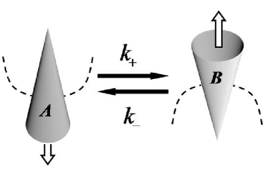
Figure 1: Schematic representation of the model. Placed in one of the layers of the membrane, the two constituents constituents $A$ and $B$ induce positive and negative curvatures, respectively (dashed lines). The species are interconverted by means of a nonequilibrium reaction: $k_{+}$ and $k_{-}$ are the forward and backward rate constants, respectively. The mechanical effect of the reactive process on the membrane shape is illustrated by the hollow arrows.

We write Eqs. (2a) and (2b) in detail in terms of dimensionless parameters where the energy is measured in units of the thermal energy $k_{B}T$, the time in units of $\tau_{h}$, and length in units of $\sqrt{D\tau_{h}}$:

$$\frac{\partial\phi}{\partial t} = (\kappa H_{0}^{2}-\alpha)\nabla^{2}\phi+3\beta\phi^{2}\nabla^{2}\phi+6\beta\phi|{\mathbf{\nabla}}\phi|^{2}$$ (3a)

$$~{}~{}-\gamma\nabla^{4}\phi-\kappa H_{0}\nabla^{4}h-\Gamma\left(\phi-\phi_{0}\right),$$

$$\frac{\partial h}{\partial t} = -\kappa\nabla^{4}h+\kappa H_{0}\nabla^{2}\phi+\Gamma(\phi-\phi_{0})\xi.$$ (3b)

In the next two sections we show analytically and confirm numerically that the new force term can have profound effects on the instability and pattern formation properties of the model. In particular, this term may lead to dynamical patterns, whereas in its absence only stationary patterns are possible.

III Analytical treatments

The stationary uniform state corresponds to $\overline{\phi}=\phi_{0}$ and arbitrary $\overline{h}$. The linear stability of these uniform solutions is tested by adding small plane-wave perturbations of wave numer $q$ to the uniform state and linearizing Eqs. (3a) and (3b) in these perturbations. This procedure leads to the $2\times 2$ linearization matrix ${\mathcal{L}}$ with the following coefficients,

$${\mathcal{L}}_{11} = -q^{2}\left[\left(\kappa H_{0}^{2}-\alpha+3\beta\phi_{0}^{2}\right)+\gamma q^{2}\right]-\Gamma$$

$${\mathcal{L}}_{12} = -\kappa H_{0}q^{4}$$

$${\mathcal{L}}_{21} = -\kappa H_{0}q^{2}+\Gamma\xi$$

$${\mathcal{L}}_{22} = -\kappa q^{4}.$$ (4)

The eigenvalues $\omega_{q}$ of the Jacobian associated with the matrix ${\mathcal{L}}$ correspond to the linear growth rates of the perturbations.

The solutions of the eigenvalue problem are given by $\omega_{q}=\frac{1}{2}\left(Tr[{\mathcal{L}}]\pm\sqrt{\Delta[{\mathcal{L}}]}\right)$, where $\Delta[{\mathcal{L}}]=Tr[{\mathcal{L}}]^{2}-4Det[{\mathcal{L}}]$. At the instability boundary, ${\rm Re}(\omega_{q})$ vanishes for one finite wave number that is defined as the first unstable mode. If the imaginary part of $\omega_{q}$ is not zero at this wave number, we have a wave bifurcation. The condition for this bifurcation is obtained by requiring $Tr[{\mathcal{L}}]=0$ and $\Delta[{\mathcal{L}}]<0$. If the imaginary part of the growth rate is zero, one has a Turing-like bifurcation. The condition for this bifurcation is $Det[{\mathcal{L}}]=0$.

In the absence of the interconversion reaction it is of course well known that immiscibility leads to complete phase separation. This occurs because a continuous range of modes starting from $q=0$ is unstable, and phase separation does not stop until there is complete segregation into two large domains. In our previous work primer we showed that the interconversion reaction provides a mixing mechanism that stabilizes the longest wavelength modes. If the reaction rate parameter $\Gamma$ is sufficiently large,

$$\Gamma>\Gamma_{1}=\frac{\left(\alpha-3\beta\phi_{0}^{2}\right)^{2}}{4\gamma},$$ (5)

then mixing is complete, the instability disappears, and the bilayer becomes stable and essentially flat. If $\Gamma<\Gamma_{1}$, the reaction no longer stabilizes all modes, but it does stabilize the longest wave vector modes. The first mode to become unstable is

$$q^{2}_{1}=\frac{\alpha-3\beta\phi_{0}^{2}}{2\gamma}=\sqrt{\frac{\Gamma_{1}}{\gamma}}.$$ (6)

The longest wavelength unstable mode now lies at the finite value

$$q_{min}^{2}=\frac{\alpha-3\beta\phi_{0}^{2}}{2\gamma}-\frac{1}{2\gamma}\sqrt{(\alpha-3\beta\phi_{0}^{2})^{2}-4\gamma\Gamma}.$$ (7)

This means that the phase separation process stops when the separated regimes are of characteristic size $\sim q_{min}^{-1}$. The patterns are Turing-like (stationary) because the imaginary part of the growth rate is zero at the bifurcation point. A typical phase diagram found earlier for this case is shown in Fig. 2. Note that the pattern size is independent of curvature parameters. Curvature reduces the unstable mode growth rates (see the $\xi=0$ curves in Fig. 3), but without changing either the characteristic size of the patterns nor the marginal condition (5). The effect of curvature is thus restricted to the kinetics of the phase separation process, as has been extensively analyzed in primer .

Figure 2: Phase diagram for the case of immiscible components in the plane $(\alpha,\Gamma)$ for $\gamma=1$ and $\phi_{0}=0$ when there is no force on the membrane caused by the interconversion reaction. From primer .

Figure 3: Dispersion relation functions $\omega_{q}$ for different values of $\Gamma$ and $\xi$. The other parameters are held fixed at $\alpha=\gamma=1$, $\phi_{0}=0$, $\kappa=0.5$ and $H_{0}=0.2$. Only the case with $\xi=5$ has a nonzero imaginary part of the dispersion relation (plotted with symbols).

The new questions of interest here are the consequences of the reaction–shape coupling in the kinetic equations. To place the analytic results obtained in this section in context, we anticipate the numerical results of the next section and exhibit two different views of a typical phase diagram in Fig. 4. Regime III is the stable regime where the mixing due to the interconversion is sufficiently strong to produce a homogeneous phase. Here “sufficiently strong” depends on the value of the parameter $\xi$. Beyond this stable regime, there are now two instability regimes. One, called region II in the diagrams, is the Turing instability regime leading to stationary nonequilibrium patterns, that is, the same sorts of patterns observed in the absence of the reaction–shape coupling (upper region of Fig. 2) primer . The condition for the Turing-like bifurcation, $Det[{\mathcal{L}}]=0$, obtained from the linear stability conditions now is $\Gamma<\Gamma_{2}$, with

$$\Gamma_{2}=\frac{\left(\alpha-3\beta\phi_{0}^{2}\right)^{2}}{4\gamma\left(1+H_{0}\xi\right)}.$$ (8)

This is the curve bounding region II in the figure. The first Turing-like unstable mode occurs at

$$q^{2}_{2}=\frac{\alpha-3\beta\phi_{0}^{2}}{2\gamma}=\sqrt{\frac{\Gamma_{2}\left(1+H_{0}\xi\right)}{\gamma}}.$$ (9)

Figure 4: Phase diagrams in the planes $(\alpha,\Gamma)$ for $\xi=5$, and $(\xi,\Gamma)$ for $\alpha=1$. The other parameter values are $\gamma=1$, $\kappa=0.5$, $H_{0}=0.2$ and $\phi_{0}=0$. The boundaries in these diagrams have been calculated numerically (see Sec. IV).

The new regime, region I, is one in which one observes dynamical (i.e., time-dependent) patterns. Provided the reaction parameter is sufficiently small and the reaction–shape coupling parameter is sufficiently large, the linear stability analysis in this regime leads to wave bifurcation solutions, $Tr[{\mathcal{L}}]=0$ and $\Delta[{\mathcal{L}}]<0$. The explicit conditions for these time dependent solutions obtained from the linear stability conditions are $\Gamma<\Gamma_{0}$, with

$$\Gamma_{0}=\frac{\left(\alpha-3\beta\phi_{0}^{2}-\kappa H_{0}^{2}\right)^{2}}{4\left(\gamma+\kappa\right)},$$ (10)

and $\xi>\xi_{0}$, with

$$\xi_{0}=\frac{\kappa q^{2}_{0}}{\Gamma H_{0}}\left(H_{0}^{2}+q^{2}_{0}\right).$$ (11)

The first unstable mode in the above expression now is

$$q^{2}_{0}=\frac{\alpha-3\beta\phi_{0}^{2}-\kappa H_{0}^{2}}{2\left(\gamma+\kappa\right)}=\sqrt{\frac{\Gamma_{0}}{\gamma+\kappa}}.$$ (12)

The curves bounding region I in Fig. 4 arise from these expressions. A typical dispersion relation function $\omega(q)$ in this regime is shown in Fig. 3. The function now has a nonzero imaginary part as well as a real part, as appropriate for spatiotemporal pattern formation. Typical spatiotemporal field configurations in the unstable regions of the phase diagram can only be found numerically. We do so in the next section.

Before doing so, however, we can go a step further in the analytic approach to the problem by introducing a weakly nonlinear analysis based on the amplitude equation formalism. Such a nonlinear expansion is valid near the bifurcation threshold to pattern formation and sheds light on the expected pattern configurations and their dynamical properties. For simplicity, we restrict the calculation of the amplitude equations to one spatial dimension. Nonetheless, we can readily deduce the possible arrangements in two dimensions by an appropriate interpretion of the coupling terms.

The details of the derivation of the amplitude equations are presented in the Appendix. The analysis reveals that a solution for equations (3a) and (3b) near the bifurcation to pattern formation reads

$$\phi(x,t) = \phi_{0}+A_{+}(x,t)\exp\left[i(q_{0}x+\omega_{0}t)\right]$$ (13a)

$$+A_{-}(x,t)\exp\left[i(q_{0}x-\omega_{0}t)\right]+c.c.,$$

$$h\left(x,t\right) = B_{+}(x,t)\exp\left[i(q_{0}x+\omega_{0}t)\right]$$ (13b)

$$+B_{-}(x,t)\exp\left[i(q_{0}x-\omega_{0}t)\right]+c.c.,$$

where $c.c.$ stands for the complex conjugate, $\omega_{0}=\left|{\rm Im}(\omega_{q_{0}})\right|$, and the amplitudes $A_{\pm}(x,t)$ and $B_{\pm}(x,t)$ satisfy the equations

$$\frac{\partial A_{\pm}}{\partial t} = (\Gamma_{0}-\Gamma)A_{\pm}-\frac{3\beta q_{0}^{2}(\Gamma_{0}-\Gamma)}{\Gamma_{0}}$$ (14a)

$$\times \left(1-\frac{24\beta\phi_{0}^{2}q_{0}^{2}(8\kappa q_{0}^{4}+i\omega_{0})}{c_{1}}\right)A_{\pm}\left|A_{\pm}\right|^{2}$$

$$-c_{2}A_{\pm}\left|A_{\mp}\right|^{2}$$

$$+(3\beta\phi_{0}^{2}+H_{0}^{2}\kappa+6\gamma q_{0}^{2}-\alpha)\frac{\partial^{2}A_{\pm}}{\partial x^{2}}$$

$$+6H_{0}\kappa q_{0}^{2}\frac{\partial^{2}B_{\pm}}{\partial x^{2}},$$

$$\frac{\partial B_{\pm}}{\partial t} = -\xi(\Gamma_{0}-\Gamma)A_{\pm}$$ (14b)

$$+H_{0}\kappa\frac{\partial^{2}A_{\pm}}{\partial x^{2}}+6\kappa q_{0}^{2}\frac{\partial^{2}B_{\pm}}{\partial x^{2}},$$

where

$$c_{1} = 8\kappa q_{0}^{4}\left[\Gamma_{0}(1+H_{0}\xi)+4q_{0}^{2}(3\beta\phi_{0}^{2}+4\gamma q_{0}^{2}-\alpha)\right]-2\omega_{0}^{2}$$

$$-i\omega_{0}\left[\Gamma_{0}+4q_{0}^{2}\left(3\beta\phi_{0}^{2}+H_{0}^{2}\kappa-\alpha+4q_{0}^{2}(\gamma+\kappa)\right)\right),$$

$$c_{2} = \frac{6\beta q_{0}^{2}(\Gamma_{0}-\Gamma)}{\Gamma_{0}}$$

$$\times \left(1-\frac{24\beta\phi_{0}^{2}q_{0}^{2}}{\Gamma_{0}(1+H_{0}\xi)+4q_{0}^{2}(3\beta\phi_{0}^{2}+4\gamma q_{0}^{2}-\alpha)}\right).$$

Note that no pattern develops if $\Gamma>\Gamma_{0}$ since the amplitudes then decay with time, $A_{\pm},B_{\pm}\rightarrow 0$. Note also the coupling term between the rightward, $A_{-}$, and leftward, $A_{+}$, traveling waves. This interaction is responsible for generating either standing or traveling waves in the membrane dynamics. Standing waves appear as a result of a kink-antikink dynamics where both waves have the same amplitude, $A_{-}=A_{+}$. Traveling waves require these amplitudes to be different. Therefore, if the coefficient $c_{2}$ of this interaction term is small (strictly speaking, zero) we expect the two amplitudes to be equal, so that

$$\phi(x,t) = \phi_{0}+4A_{+}(x,t)\cos(q_{0}x)\cos(\omega_{0}t),$$ (16a)

$$h(x,t) = 4B_{+}(x,t)\cos(q_{0}x)\cos(\omega_{0}t),$$ (16b)

that is, the solution is a standing wave. On the other hand, if $c_{2}$ is not zero, a traveling wave appears. Observe that if $\phi_{0}=0$, that is, if the composition of the membrane is 50% lipid $A$ and 50% lipid $B$, then the $A_{+}\leftrightarrow A_{-}~{}$interaction term is always relevant and no standing waves are possible. This scenario is confirmed by the numerical simulations described in the next section (cf. Figs. 5 and 6, where we see a composition-curvature traveling wave in the membrane. For the parameters in that figure, $c_{2}\approx 0.25$). On the other hand, this restriction does not apply if the membrane composition is such that $\phi_{0}\neq 0$ (cf. Figs. 7 and 8, where $\phi_{0}=0.14$ and $c_{2}\approx$ $10^{-2}$; the simulations show that in those cases there is a standing oscillatory contribution to the pattern). As for the different spatial configurations, one obtains either rolls or hexagons depending on the symmetries of the system. Thus, note that in Eqs. (3a) and (3b) the inversion symmetry

$$\phi\rightarrow-\phi,\qquad h\rightarrow-h$$ (17)

is satisfied only if $\phi_{0}=0$ and in that case roll-like arrangements are obtained. On the other hand, if $\phi_{0}\neq 0$ there is no inversion symmetry, and the resulting structures are expected to be hexagonal.

IV Numerical Results

Representative numerical results are presented in this section, showing good agreement with the predictions of the linear stability and amplitude equation analyses. We numerically solve Eqs. (3a) and (3b) in a two-dimensional square lattice of $100\times 100$ sites with a mesh size $\Delta x=1$ and periodic boundary conditions. The spatial derivatives are calculated by means of a simple centered scheme, and a first-order Euler algorithm with time step $\Delta t=10^{-4}$ is used for the temporal integration. These coordinate and time steps insure good numerical accuracy. Simulations are started from a slightly randomly perturbed homogeneous distribution $\phi(\vec{r})=\overline{\phi}=\phi_{0}$ and $h(\vec{r})=\overline{h}=0$. In this section we present numerical results that correspond to highly immiscible components (deep quench, $\alpha=1$ and $\beta=1$, leading to an equilibrium value of $\phi_{eq}=\pm 1$), and an interface thickness of the order of the space discretization ($\zeta=1$, which leads to $\gamma=1$). The bending rigidity modulus is taken equal to $0.5$ (in units of $k_{B}T$), and very different shapes are implemented for the two constituents by setting $H_{0}=0.2$.

When dealing with mesosopic or coarse-grained modeling schemes one has to be concerned about the applicability of the results. The limit on the predictive power of these models is mainly determined by the identification of the correct time, length and energy scales accessible to the experiments. In our case, we have adimensionalized the kinetic equations in order to have $D=\Lambda=k_{B}T=1$, so we can return dimensions to these equations by choosing typical values for these parameters. The diffusion coeficient is known to be in the range $10^{-7}-10^{-8}$cm²/s (for lipids in a liquid-disordered phase membrane hous ). In the absence of the nonlinear and mechanical effects considered in this paper, solvent hydrodynamic effects (Zimm dynamics) seif can be incorporated with a renormalized height mobility $\Lambda=\left(4\mu q\right)^{-1}$ in Eq. (2b) in Fourier space frey . Here $\mu$ stands for the solvent kinematic viscosity, which is $1$cp for water at $20^{\circ}$C. For $\kappa=0.5k_{B}T$ the linear stability analysis shows typical unstable modes at $q\approx q_{0}\approx 0.5$, which corresponds to a pattern size in the range of $2-20\mu$m. Such a size may be accessible in experiments on giant vesicles and planar bilayers. However, when mechanical effects are included, a more elaborate analysis such as that provided by dynamical renormalization methods frey is in order. A simple and plausible hypothesis might be to include such effects by simply renormalizing both $\Lambda$ and $\xi$ in Eq. (2b), both with a $1/q$ decay in Fourier space since one might expect a non-local viscous kernel to decay as a power law with distance moldovan . In any case, a more detailed consideration of this issue is beyond the scope of this work.

Figure 5: Spatiotemporal behavior for the case of an unstable membrane in region I of the pase diagram Fig. 4 and the following set of parameters: $\alpha=\beta=\gamma=1$, $\phi_{0}=0$, $\kappa=0.5$, $H_{0}=0.2$, $\Gamma=0.14$ and $\xi=5$ (dashed curve in Fig. 3). The two upper panels correspond to the $\phi$- and $h$-field distributions at $t=15000$, once the structures are robust. The stripes travel from left to right at constant velocity. In the third panel we plot the temporal evolution (horizontal axis) of a one-dimensional cross-section $\phi$-profile (vertical axis) at $y=50$, starting at $t=15000$ until $t=19000$. In the fourth panel, the corresponding $h$-profile (horizontal axis) is plotted against time (downward below sheet axis), starting at $t=15000$ until $t=15500$. Darker (lighter) regions are richer in the $A$ ($B$) lipid in the concentration snapshots, and some exaggeration along the vertical direction has been applied to the height plots.

Figure 6: $\phi$- and $h$-profiles for the case in Fig. 5 at a given time $t=18000$. The arrow represents the direction of propagation of the traveling pattern.

However, in order to accurately delimit the range of applicability of our model, it is useful to add some comments regarding the value of $\kappa$. The elastic properties, and thus the bending rigidity, of lipid bilayers are strongly determined by the size, shape and molecular elasticity of their constituents. Membranes composed of phospholipids (which have two hydrophobic chains) are characterized by a bending rigidity of the order of tens of $k_{B}T$ kapa . Cell membranes containing large molar fractions of cholesterol (rather rigid molecules) display even higher rigidities lenon . In our model, the typical sizes of the predicted dynamical patterns emerging from a wave instability for such large values of $\kappa$ exceed the experimentally accessible sizes. Moreover, for $\kappa\gtrsim 10$, wave-like unstable modes are observed to be supressed at long times by the other existing Turing-like unstable modes, so that only stationary structures are asymptotically generated in this parameter region. However, single- and/or short-chain lipid surfactants are known to form much more flexible bilayers, with bending rigidities of the order of $k_{B}T$ or even less lowkapa . Furthermore, recent theoretical models lowklip show how bilayers composed of surfactants of rather distinct shapes (as in our case) may exhibit smaller rigidities than one-component membranes. This, therefore, delimits the range of applicability of the model results in this paper.

Our quantitative assigment of $\xi$ has been made with the energetic feasibility of a number of external sources in mind. To see this, note that the characteristic time for a single reactive event is of order $1/\Gamma$. During this time interval the change in the height of the membrane due to the contribution of the reactive term is of order $~{}\xi$ [see. Eq. (2b); $\phi-\phi_{0}$ is of $O(1)$]. Moreover, the local energetic “cost” of such a height increase due to the reactive term is of order $2\kappa\xi^{2}/(\Delta x)^{2}$ [see Eq. (1)]. In most of our simulations we have used $\xi=5$ (in simulation length units), which, for $\kappa=0.5$, corresponds to an energy cost of order $25$ (in units of $k_{B}T$). The dephosphorylation of an ATP releases about $50$kJ/mol or $10^{-19}$J/ATP, which at room temperature is precisely of order $25k_{B}T$. If the energy source is light, the power required to produce $25k_{B}T$ within a time interval of order $\Gamma^{-1}$ for $\Gamma=0.14$ as used in our simulations is only approximately $0.3\times 10^{-6}$mW/cm², which is much lower than the power produced by typical commercial light sources used, for example, in photosensitive Langmuir monolayer experiments. While some of the energy provided by these external sources (ATP, light, etc.) would be used for processes other than the purely elastic motion of the membrane, including dissipation into the thermal surroundings and the movement of other masses, this order of magnitude estimate shows that the mechanism is feasible and provides a basis for the value of the parameter $\xi$ chosen for our simulations.

For a highly flexible bilayer, typical phase diagrams are those of Fig. 4. As noted earlier, region I corresponds to a regime where at least one of the unstable modes has nonzero imaginary part, so both types of instablity are present. Region II is the unstable phase also present in Fig. 2. Here, the unstable modes have no imaginary parts, so that stationary finite-sized patterns are predicted. In region III, there are no unstable modes (stable phase). Here we have exhibit spatiotemporal patterns associated with the new region I.

The nature of the spatiotemporal patterns is determined by the value of $\phi_{0}$ and by the associated relative magnitudes of the amplitudes of waves traveling in different directions. These assertions are supported by the amplitude equation analysis of the previous section. Thus, for a critical quench ($\phi_{0}=0$), the system typically displays some transients with domains that travel in different directions until they organize into a coherent train of traveling stripes. The post-transient spatiotemporal behavior is described in the different panels in Fig. 5. We plot the concentration and height fields (upper panels), and one-dimensional cross-sections showing the temporal evolution, for both order parameters. The traveling waves are consistent with the predictions of the amplitude equation analysis. Numerical profiles at a given post-transient stage reveal the mechanism that leads to the motion of the generated spatial structures. In Fig. 6 we observe that $\phi$- and $h$-profiles are slightly displaced, the field $\phi$ being ahead in the direction of propagation. That there is such a phase difference between the two fields is consistent with the appearance of the contribution with an imaginary coefficient on the right hand side of Eq. (14b).

Off-critical quenches ($\phi_{0}=-0.14$) display different spatial and temporal behaviors, again consistent with the amplitude equation results. As before, we first observe transients, but now involving concentration droplets and bud-like surface deformations. The fields settle into an oscillating pattern of buds rich in the minority species and whose geometry depends on the value of the parameter $\xi$ that measures the mechanical effect of the reaction on the shape of the membrane. This behavior is shown in Fig. 7. For $\xi=5$ a spatial Fourier transform of the pattern indicates clear square symmetry. For $\xi=3$, the domains are rather hexagonal and they oscillate as well as move in one direction, as shown in Fig. 8.

Figure 7: Spatiotemporal behavior for the same case as in Fig. 5 except for $\phi_{0}=-0.14$ (still in region I). The snapshots correspond to $t=22500$ and the temporal profile evolutions go from this time up to $t=26500$ for $\phi$, and to $t=23000$ for $h$. The same panel organization and specifications as in Fig. 5 apply. Bud-like curvature domains oscillate.

Figure 8: Spatiotemporal behavior for the same case in Fig. 5 except for $\phi_{0}=-0.14$ and $\xi=3$ (still in region I). In the upper panels, the droplet-like structures move from the upper-left corner to the lower-right one at constant velocity, while they oscillate. The snapshots correspond to $t=18000$ and the temporal profile evolutions go from this time up to $t=22000$ for $\phi$, and to $t=18500$ for $h$. The same panel organization and specifications as in Fig. 5 apply.

V Conclusions

In a previous model for a flexible reactive bilayer composed of two differently shaped lipids, we demonstrated the occurrence of stationary finite-sized domains of composition and curvature as a result of the competition between thermodynamic phase segregation and a nonequilibrium reaction primer . A generalization of the model that includes the local effect of the reaction on the membrane shape has been presented here. We have shown how the mechanical influence of the reactive process on the membrane may lead to the formation of spatiotemporal structures. The linear stability analysis of the model equations shows the existence of a wave instability for sufficiently large reaction–shape coupling. A weakly nonlinear analysis based on the amplitude equation formalism provides insight into the spatial and temporal symmetries of the emerging patterns. Correspondingly, numerical simulations display the spontaneous generation of traveling lamelar phases, and oscillating or moving buds, showing an important potential for the formation of spatiotemporal patterns in deformable nonequilibrium reactive lipid membranes.

This extension of the model should be considered as a formal issue in reactive deformable surfaces. However, we believe that experimental work on giant vesicles and on planar membranes can be designed to qualitatively capture the spatiotemporal phenomenology obtained in our model. Azobenzene derivatives, which are also known to display dynamical organization in nonequilibrium Langmuir monolayers our , may be suitable compounds to test our predictions since their shapes can be strongly modified by means of well-known (externally controlled) photoisomerization reactions rau , and the resulting isomers normally exhibit phase separation.

Finally, we note that it would be interesting to study the crossover between Rouse and Zimm dynamics in our model system so as to elucidate how the different parameters are renormalized due to solvent hydrodynamic effects, and to clarify the resulting consequences for the pattern formation mechanism proposed herein. Such a study has been carried out for tethered membranes, where different coarsening exponents are found frey ; moldovan .

Appendix A Derivation of the amplitude equations

For convenience of notation, we rewrite the one dimensional version of the model equations (3a) and (3b) for reactive membranes in terms of the shifted field variable $\varphi=\phi-\phi_{0}$ and the control parameter $\varepsilon=(\Gamma_{0}-\Gamma)/\Gamma_{0}$ that accounts for the “distance” to the threshold of the bifurcation to pattern formation so that a pattern develops if $\varepsilon>0$:

$$\varphi_{t} = (\kappa H_{0}^{2}-\alpha)\varphi_{xx}+3\beta(\varphi+\phi_{0})\varphi_{xx}$$ (18a)

$$+6\beta(\varphi+\phi_{0})\left(\varphi_{x}\right)^{2}-\gamma\varphi_{xxxx}$$

$$-\kappa H_{0}h_{xxxx}-\Gamma_{0}(1-\varepsilon)\varphi,$$

$$h_{t} = -\kappa h_{xxxx}+\kappa H_{0}\varphi_{xx}+\xi\Gamma_{0}(1-\varepsilon)\varphi.$$ (18b)

The subscripts indicate partial derivatives. The homogeneous state is $\varphi=0$ and arbitrary $h=\bar{h}$. With no loss of generality we take $\bar{h}=0$.

Slightly above the bifurcation to pattern formation, the following expansion holds (see primer ; hecke and references therein):

$$\varphi = \sum_{n=1}^{\infty}\varepsilon^{n/2}\varphi^{(n)},$$ (19a)

$$h = \sum_{n=1}^{\infty}\varepsilon^{n/2}h^{(n)},$$ (19b)

and a separation of spatial scales can be implemented between the most unstable mode (fast growth), $q_{0}$, and the rest of the modes within the unstable band (slower growth). In terms of the control parameter, we let $X=\varepsilon^{1/2}x$ denote the spatial modulation scale of the slow modes and $T=\varepsilon t$ the associated time scale. The separation of scales between the fastest growing mode and the slower modes can be implemented in Eqs. (18a) and (18b) by expanding the spatial and temporal derivatives according to the chain rule so that $\partial_{x}\rightarrow\partial_{x}+\varepsilon^{1/2}\partial_{X}$ and $\partial_{t}\rightarrow\partial_{t}+\varepsilon\partial_{T}$. Implementation of this scale separation and substitution of Eqs. (19a) and (19b) into (18a) (18b) leads to a rather cumbersome expansion in terms of $\varepsilon$. The lowest order contribution is of order $\varepsilon^{1/2}$, and balancing all terms of this order gives

$$(3\beta\phi_{0}^{2}+H_{0}^{2}\kappa-\alpha)\varphi_{xx}^{(1)}-\gamma\varphi_{xxxx}^{(1)}-\Gamma_{0}\varphi^{(1)}$$

$$~{}~{}~{}~{}~{}~{}-H_{0}\kappa h_{xxxx}^{(1)}-\varphi_{t}^{(1)}=0,$$ (20a)

$$\xi\Gamma_{0}\varphi^{(1)}+H_{0}\kappa\varphi_{xx}^{(1)}-\kappa h_{xxxx}^{(1)}-h_{t}^{(1)}=0.$$ (20b)

Equations (20a) and (20b) are in fact simply the linearized versions of Eqs. (18a) and (18b). With the definition of the linear operator $\mathbb{L}$ with elements

$$\mathbb{L}_{11} = (3\beta\phi_{0}^{2}+H_{0}^{2}\kappa-\alpha)\frac{\partial^{2}}{\partial x^{2}}-\gamma\frac{\partial^{4}}{\partial x^{4}}-\Gamma_{0}-\frac{\partial}{\partial t}$$

$$\mathbb{L}_{12} = -H_{0}\kappa\frac{\partial^{4}}{\partial x^{4}}$$

$$\mathbb{L}_{21} = \xi\Gamma_{0}+H_{0}\kappa\frac{\partial^{2}}{\partial x^{2}}$$

$$\mathbb{L}_{22} = -\kappa\frac{\partial^{4}}{\partial x^{4}}-\frac{\partial}{\partial t},$$

Eqs. (20a) and (20b) can trivially be written as $\mathbb{L}\mathbf{\chi}_{1}=0$, where $(\mathbf{\chi}_{n})^{T}=\left(\varphi^{(n)},h^{(n)}\right)$.

The next order of the expansion gives us terms of $\mathcal{O}(\varepsilon)$ and yields $\mathbb{L}\mathbf{\chi}_{2}=\mathbf{\psi}_{2}\left(\left\{\varphi^{(1)};h^{(1)}\right\}\right)$, where $\mathbf{\psi}_{2}^{T}=\left(\mathbf{\psi}_{2}^{(a)}\mathbf{,\psi}_{2}^{(b)}\right)$, and

$$\mathbf{\psi}_{2}^{(a)} = -6\beta\phi_{0}\left[\left(\varphi_{x}^{(1)}\right)^{2}+\varphi^{(1)}\varphi_{xx}^{(1)}\right)$$

$$+2\left(\alpha-3\beta\phi_{0}^{2}-H_{0}^{2}\kappa\right)\varphi_{xX}^{(1)}+4\gamma\varphi_{xxxX}^{(1)}$$

$$+4H_{0}\kappa h_{xxxX}^{(1)},$$

$$\mathbf{\psi}_{2}^{(b)} = 2\kappa\left(-H_{0}\varphi_{xX}^{(1)}+2h_{xxxX}^{(1)}\right).$$

At order $\varepsilon^{3/2}$ we get $\mathbb{L}\mathbf{\chi}_{3}=\mathbf{\psi}_{3}\left(\left\{\varphi^{(1)},\varphi^{(2)};h^{(1)},h^{(2)}\right\}\right)$, where the components of $\mathbf{\psi}_{3}^{T}=\left(\mathbf{\psi}_{3}^{(a)}\mathbf{,\psi}_{3}^{(b)}\right)$ are given by

$$\mathbf{\psi}_{3}^{(a)} = \varphi_{T}^{(1)}-\Gamma_{0}\varphi^{(1)}$$

$$-6\beta\varphi_{x}^{(1)}\left(\varphi^{(1)}\varphi_{x}^{(1)}+2\phi_{0}\left(\varphi_{X}^{(1)}+\varphi_{x}^{(2)}\right)\right)$$

$$+\left(\alpha-H_{0}^{2}\kappa\right)\left(\varphi_{XX}^{(1)}+2\varphi_{xX}^{(2)}\right)$$

$$-3\beta\left\{\phi_{0}^{2}\left(\varphi_{XX}^{(1)}+2\varphi_{xX}^{(2)}\right)\right.$$

$$\left.+\varphi_{xx}^{(1)}\left[\left(\varphi^{(1)}\right)^{2}+2\phi_{0}\varphi^{(2)}\right]\right.$$

$$\left.+2\phi_{0}\varphi^{(1)}\left(2\varphi_{xX}^{(1)}+\varphi_{xx}^{(2)}\right)\right\}$$

$$+2\gamma\left(3\varphi_{xxXX}^{(1)}+2\varphi_{xxxX}^{(2)}\right)$$

$$+2H_{0}\kappa\left(3h_{xxXX}^{(1)}+2h_{xxxX}^{(2)}\right),$$

$$\mathbf{\psi}_{3}^{(b)} = h_{T}^{(1)}+\xi\Gamma_{0}\varphi^{(1)}+\kappa\left[2\left(3h_{xxXX}^{(1)}+2h_{xxxX}^{(2)}\right)\right.$$

$$\left.-H_{0}\left(\varphi_{XX}^{(1)}+2\varphi_{xX}^{(2)}\right)\right].$$

We could continue up to any order with the expansion. However, at order $\varepsilon^{3/2}$ we are able to extract a closed evolution equation for the amplitudes of the pattern, as shown below, and we therefore stop at this order. Note that beyond order $\varepsilon^{1/2}$, which corresponds to the linear problem, in all cases we obtain a non-homogeneous equation, such that at order $\varepsilon^{n/2}$

$$\mathbb{L}\mathbf{\chi}_{n}=\mathbf{\psi}_{n}\left(\left\{\varphi^{(1)},\ldots,\varphi^{(n-1)};h^{(1)},\ldots,h^{(n-1)}\right\}\right).$$ (21)

At order $\varepsilon^{1/2}$ the problem is homogeneous and, with appropriate boundary conditions, we can write the solution as

$$\varphi^{(1)} = A_{1+}(X,T)e^{i(q_{0}x+\omega_{0}t)}$$ (22a)

$$+A_{1-}(X,T)e^{i(q_{0}x-\omega_{0}t)}+c.c.,$$

$$h^{(1)} = B_{1+}(X,T)e^{i(q_{0}x+\omega_{0}t)}$$ (22b)

$$+B_{1-}(X,T)e^{i(q_{0}x-\omega_{0}t)}+c.c.,$$

where $c.c.$ stands for the complex conjugate and $\omega_{0}=\left|{\rm Im}(\omega_{q_{0}})\right|$. However, the amplitudes $A_{1\pm}$ and $B_{1\pm}$ are undetermined at this point. As mentioned above, the subsequent orders are no longer homogeneous and therefore the existence of an analytical solution can not be ensured. However, we can enforce solvability by evoking the Fredholm alternative theorem newell . In our case the application of the theorem simply states, as a recipe, that for Eqs.(21) to have a solution, the functions $\psi_{n}$ can not contain the fundamental mode $\exp\left[\pm\left(iq_{0}x\pm\omega_{0}t\right)\right]$. In other words, the particular solutions of the non-homogeneous problem are orthogonal to the solutions of the homogeneous problem. Thus, by substituting the solutions (22a) and (22b) into the next order of the hierarchy and imposing the solvability condition we obtain the following particular solution,

$$\varphi^{(2)} = c_{1\varphi}\left[A_{1+}(X,T)\right]^{2}e^{2i(q_{0}x+\omega_{0}t)}$$

$$+c_{2\varphi}\left[A_{1-}(X,T)\right]^{2}e^{2i(q_{0}x-\omega_{0}t)}$$

$$+c_{3\varphi}A_{1+}(X,T)A_{1-}(X,T)e^{2iq_{0}x}+c.c.,$$

$$h^{(2)} = c_{1h}\left[\left(A_{1+}(X,T)\right)^{2}e^{2i(q_{0}x+\omega_{0}t)}\right.$$

$$\left.+\left(A_{1-}(X,T)\right)^{2}e^{2i(q_{0}x-\omega_{0}t)}\right]$$

$$+c_{2h}A_{1+}(X,T)A_{1-}(X,T)e^{2iq_{0}x}+c.c.,$$

where

$$c_{1\varphi} = \frac{c_{1\varphi}^{num}}{c_{1\varphi}^{den}}$$

$$c_{1\varphi}^{num} = \left[12\beta\phi_{0}q_{0}^{2}\left(8\kappa q_{0}^{4}+i\omega_{0}\right)\right]$$

$$c_{1\varphi}^{den} = \left[8H_{0}\kappa q_{0}^{4}(4H_{0}\kappa q_{0}^{2}-\Gamma_{0}\xi)\right.$$

$$-(8\kappa q_{0}^{4}+i\omega_{0})\left(\Gamma_{0}+4q_{0}^{2}(3\beta\phi_{0}^{2}+H_{0}^{2}\kappa\right.$$

$$\left.\left.+4\gamma q_{0}^{2}-\alpha)+2i\omega_{0}\right)\right],$$

$$c_{2\varphi} = -\frac{\left[12\beta\phi_{0}q_{0}^{2}(8\kappa q_{0}^{4}-i\omega_{0})\right]}{c},$$

$$c_{3\varphi} = -\frac{24\beta\phi_{0}q_{0}^{2}}{\Gamma_{0}(1+H_{0}\xi)+4q_{0}^{2}(3\beta\phi_{0}^{2}+4\gamma q_{0}^{2}-\alpha)},$$

$$c_{1h} = \frac{\left[6\beta\phi_{0}q_{0}^{2}\left(-\xi\Gamma_{0}+4H_{0}\kappa q_{0}^{2}\right)\right]}{c^{\ast}},$$

$$c_{2h} = -\frac{3\beta\phi_{0}q_{0}^{2}(\xi\Gamma_{0}-4H_{0}\kappa q_{0}^{2})}{2\kappa q_{0}^{4}\left[\Gamma_{0}(1+H_{0}\xi)+4q_{0}^{2}(3\beta\phi_{0}^{2}+4\gamma q_{0}^{2}-\alpha)\right]},$$

$$c = 8\kappa q_{0}^{4}\left[\Gamma_{0}(1+H_{0}\xi)+4q_{0}^{2}(3\beta\phi_{0}^{2}+4\gamma q_{0}^{2}-\alpha)\right]$$

$$-2\omega_{0}^{2}-i\omega_{0}\left[\Gamma_{0}\right.$$

$$\left.+4q_{0}^{2}\left(3\beta\phi_{0}^{2}+H_{0}^{2}\kappa-\alpha+4q_{0}^{2}(\gamma+\kappa)\right)\right],$$

and $c^{\ast}$ is the complex conjugate of $c$. The values of $A_{1\pm}$ and $B_{1\pm}$ can not be determined at this order either. However, at order $\varepsilon^{3/2}$ the Fredholm theorem provides closed equations for the conditions that must be satisfied by these amplitudes. These conditions are the amplitude equations for our pattern forming system, and are given in terms of the original variables $x$ and $t$ in Eqs. (13a) and (13b). In those equations the “1” in the subscript has been dropped for economy of notation.

References

- (1) R. Lipowsky and E. Sackmann, Structure and Dynamics of Membranes (Elsevier, Amsterdam, 1995).
- (2) R. Lipowsky, Nature 349, 475 (1991).
- (3) U. Seifert, Adv. Phys. 46, 13 (1997).
- (4) H. T. Tien, A. L. Ottova, Colloids Surf. A, 149, 217 (1999).
- (5) E. Evans and W. Rawicz, Phys. Rev. Lett. 64, 2094 (1990).
- (6) P. B. Canham, J. Theor. Biol. 26, 61 (1970).
- (7) W. Helfrich and R-M. Servuss, Nuovo Cimento D 3, 137 (1984).
- (8) L. Miao, U. Seifert, M. Wortis and H.-G. Döbereiner, Phys. Rev. E 49, 5389 (1994).
- (9) D. Andelman, T. Kawakatsu and K. Kawasaki, Europhys. Lett. 19, 57 (1992).
- (10) P. B. Sunil Kumar, G. Gompper and R. Lipowsky, Phys. Rev. E 60, 4610 (1999).
- (11) W. T. Gozdz and G. Gompper, Phys. Rev. E 59, 4305 (1999).
- (12) T. Taniguchi, Phys. Rev. Lett. 76, 4444 (1996).
- (13) P. B. Sunil Kumar and M. Rao, Phys. Rev. Lett. 80, 2489 (1998).
- (14) P. B. Sunil Kumar, G. Gompper and R. Lipowsky, Phys. Rev. Lett. 86, 3911 (2001).
- (15) M. D. Houslay and K. K. Stanley, Dynamics of Biological Membranes (Wiley, NY, 1982).
- (16) F. Brochard and J. Lennon, J. Phys. (Paris) 36, 1035 (1975).
- (17) S. Levin and R. Korenstein, Biophys. J. 60, 733 (1991).
- (18) S. Tuvia, A. Almagor, A. Bitler, S. Levin, R. Korenstein and S. Yedgar, Proc. Nat. Acad. Sci. USA 94, 5045 (1997).
- (19) J. -B. Manneville, P. Bassereau, D. Lévy and J. Prost, Phys. Rev. Lett. 82, 4356 (1999).
- (20) P. G. Petrov, J. B. Lee and H. -G. Döbereiner, Europhys. Lett. 48, 435 (1999).
- (21) S. Ramaswamy, J. Toner and J. Prost, Phys. Rev. Lett. 84, 3494 (2000).
- (22) J. -B. Manneville, P. Bassereau, S. Ramaswamy and J. Prost, Phys. Rev. E 64, 021908 (2001).
- (23) H. Wada, J. Phys. Soc. Jpn. 72, 3142 (2003).
- (24) H. -Y. Chen, Phys. Rev. Lett. 92, 168101 (2004).
- (25) S. Sankararaman, G. I. Menon and P. B. Sunil Kumar, Phys. Rev. E 66, 031914 (2002).
- (26) S. G. Ostrowski, C. T. Van Bell, N. Winograd and A. G. Ewing, Science 305, 71 (2004).
- (27) S. J. Scales and R. H. Scheller, Nature 401, 123 (1999).
- (28) S. Mann and G. A. Ozin, Nature 382, 313 (1996).
- (29) R. Reigada, J. Buceta and K. Lindenberg, Phys. Rev. E 71, 051906 (2005).
- (30) M. do Carmo, Differential Geometry of Curves and Surfaces (Prentice-Hall, Englewood Cliffs, 1976).
- (31) J. García-Ojalvo and J. M. Sancho, Noise in Spatially Extended Systems (Springer, New York, 1999) and references therein.
- (32) E. Frey and D. R. Nelson, J. Phys. I France 1, 1715 (1991).
- (33) D. Moldovan and L. Golubovic, Phys. Rev. E 60, 4377 (1999).
- (34) N. Gov, Phys. Rev. Lett. 93, 268104 (2004).
- (35) See for instance, M. Kummrow and W. Helfrich, Phys. Rev. A 44, 8356 (1991).
- (36) N. Lei and X. Lei, Langmuir 14, 2155 (1998).
- (37) A. Imparato, J. C. Shillcock and R. Lipowsky, Europhys. Lett. 69, 650 (2005).
- (38) Y. Tabe and H.Yokoyama, Langmuir 11, 4609 (1995). F. Sagués, R. Albalat, R. Reigada, J. Crusats, J. Ignés-Mullol and J. Claret, J. Am. Chem. Soc. 127, 5296 (2005).
- (39) H. Rau, Photochemistry and Photophysics, Vol II, pp. 119-141, (CRC Press, Boca Raton, Florida, 1990).
- (40) A. C. Newell, in the Proceedings of the 1988 Complex Systems Summer School, Lectures in the Sciences of Complexity Santa Fe, New Mexico, edited by D. L. Stein (Addison-Wesley, Reading, MA, 1989).
- (41) M. van Hecke, W. van Saarlos, and P.C. Hohenberg, Amplitude Equations for Pattern Forming Systems, in: Fundamental Problems in Statistical Mechanics VIII, edited by H. van Beijeren and M.H. Ernst (North Holland, Amsterdam, 1994).