Evolving network - simulation study.
From regular lattice to scale free network
Abstract
The Watts-Strogatz algorithm of transferring the square lattice to a small world network is modified by introducing preferential rewiring constrained by connectivity demand. The evolution of the network is two-step: sequential preferential rewiring of edges controlled by and updating the information about changes done. The evolving system self-organizes into stationary states. The topological transition in the graph structure is noticed with respect to . Leafy phase - a graph formed by multiple connected vertices (graph skeleton) with plenty of leaves attached to each skeleton vertex emerges when is small enough to pretend asynchronous evolution. Tangling phase where edges of a graph circulate frequently among low degree vertices occurs when is large. There exist conditions at which the resulting stationary network ensemble provides networks which degree distribution exhibit power-law decay in large interval of degrees.
PACS: 02.50.Ey, 89.75.Fb, 89.20.Ff
1 Introduction
From communication networks like World Wide Web or phone networks, through nets of social relations, namely networks of acquaintances or collaborating scientists, to biological systems where protein networks, neural networks or cell metabolisms are considered — all of them manifests a similar structural organization: small-world properties (short distances , strong clustering) and the power-law vertex degree distribution. See, e.g., [1, 2, 3, 4] for review of data analysis and bibliography. Most of these natural and man-made networks change in time. Although these networks undergo different restructuring processes, their crucial statistical properties are time independent. The networks are self-organized to stationary states. Any stationary state can be realized by many (usually huge) number of microscopically different configurations. Evolution of a stationary state denotes that microscopic changes performed do not influence the global characteristics.
In the present paper we propose a stochastic microscopic dynamic rule which leads a regular lattice into the stationary network state. By simulations we show the relation between the details of microscopic rule and the distribution of the vertex degree in a stationary state. Our proposition is based the Watts-Strogatz construction of the small-world network by rewiring edges [5].
Here, we do not consider any dynamics on a network. However, our studies are motivated by models of large spatially extended systems with short-range interactions, like Ising models, in which a spin is attached to each vertex [7, 8, 9, 10, 11, 12]. Such networks can model the magnetic nanomaterials. Electronic components are represented as vertices and the wires are edges [13]. The neural networks may also be considered as kind of electronic circuits [14, 15] following the idea of ‘save wiring’ as an organizing principle of the brain [16].
Our research is aimed on giving hints about the matter in which changes are performed on two levels. The first level means that the network topology evolves. The second level denotes that spins located in nodes are adjusted according to the new network structure. Preliminary study of such materials can be found in [17, 18, 19]. Stochastically evolving connections between at average constant number of vertices can also be viewed as the playground for modeling community structures in networks [20] or coauthorship networks [21].
The studies of the network topology began with the random graph theory of Erdös and Rényi [22]. The proposition of Watts and Strogatz [5] that followed, called small world network, captures the features of regular lattice and random graph. The algorithm may be summarized as follows: begin with a regular lattice, then rewire an edge with some probability . Traditionally, the evolution in the Watts-Strogatz network is measured by . Let us divide the process of rewiring of -part of edges into substeps such that . Hence, we can say that the - part of edges is rewired synchronously at each time step. If rewiring is stochastic, like in the Watts-Strogatz algorithm, then the resulting network after steps with -part edges rewired each time step is equivalent to a network obtained after one step with -part edges rewired. However, if rewiring goes preferentially and information about modifications introduced is updated once in a time step then different networks can be observed.
We show, by simulation, that under some conditions the resulting networks are different from networks obtained in the 1-step evolution with the corresponding . In particular, it appears that if rewiring is accompanied with ‘synchronized’ preference then the self-organization of the network state occurs. Namely, the stable vertex degree distribution is reached though the evolution of edges continuous. It is said that the ensemble of graphs emerges and the evolution walks on graphs belonging to this ensemble [23].
Moreover, we present arguments that the topological transition between the graph ensembles takes place. If values are small then, so-called, leafy phase emerges. The phase ensemble consists of graphs formed by multiple inter connected vertices, called graph skeleton, with plenty of leaves attached to each skeleton vertex. Occurrence of connections between vertices of similar properties such as, e.g., similar degrees, is termed assortativity and the high probability of connections between vertices with different degrees is termed disassortativity [23]. The strong assortativity between hubs present in the stationary state results from preferences in dynamics considered. Moreover, the vertices of the graph skeleton are surrounded by leaves, namely each hub belongs to a star-like subgraph. Hence together with strong assortativity of hubs the strong disassortativity is present also. On the other hand, if is large enough then the network stabilizes in, so-called, tangling phase where edges of a graph circulate frequently among low degree vertices.
All network ensembles are characterized by the distinct degree distributions with exponentially vanishing tails. However, when the parameters driving the network evolution are specially adjusted, then the power-law decay appears in the rather wide interval of vertex degrees. The exponent for this decay is close to what suggests strong inhomogeneity in the network.
The algorithm is presented in Section 2. Section 3 contains results obtained by simulations. The discussion and development of the model is proposed in Section 4.
2 Algorithm
Let us number vertices of the lattice as . Then each edge is characterized by the two numbers (, ) representing two vertices linked by this edge. The graph is represented as the vector of size of lists of vertices — neighbors of subsequent vertices. The graph is not considered as directed, though the algorithm can easily be adapted to a directed one.
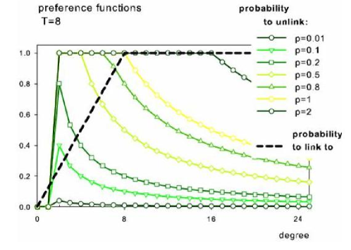
There are two basic parameters in the model: — probability to rewire an edge each time step, and — threshold in the preference function.
The synchronized preferential rewiring step means:
-
1.
Choose at random any of nodes. For the node chosen the set of its edges is reviewed. The following decisions are made:
(i) the subset of edges to rewire is selected with probability calculated as follows, see Fig. 1:(ii) for each selected to rewire the new attachment is assigned with probability to link to -node given by
-
2.
The global information on the vertex degrees is updated.
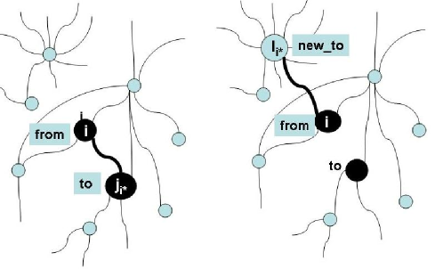
Since there are possible differences in applying Watts-Strogatz idea of rewiring, below we give the evolution procedure. The basic procedure, called, EdgeEvolution, requires three parameters: , and . The illustration of the networks before (left graph) and after(right graph) rewiring is shown in Fig. 2.
.
EdgeEvolution ( , , ) :
(a)for each vertex from the list of edges of the vertex
do
(b) if deg then
(c) choose at random and
(d) if then accept the vertex
for
(e)for each vertex accepted for
(f) choose at random but
(g) choose at random and
(h) if then accept , i.e.,
(i) otherwise go to (f)
Remarks:
— The algorithm conserves both the number of vertices and the number of edges. Steps (a)–(d) prepare the list of edges of the vertex to be rewired, while steps (f)–(i) fix new connections. Each edge accepted for rewiring must be rewired (see the loop(i)).
— The condition (b) is introduced to avoid presence of zero-degree vertices. Any vertex with a degree equal to 1 cannot be unlinked. Otherwise we face the problem of dramatically increasing number of isolated nodes. However, this condition does not protect a graph from being disconnected.
— A randomly selected new vertex for linking to must be different from the vertex to avoid loops in a graph, line (f), however, multiple edge links are not forbidden.
— Since information regarding the vertex degree is updated after each time step, hence if the network is evolving with small , then the evolution may be seen as asynchronous.
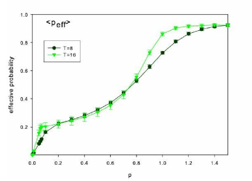
— If deg then the probability to unlink from the vertex is equal to while if deg (deg) then probability to unlink is greater (smaller, respectively) than . Therefore, the rewiring goes with some effective probability . The mean values of are shown in Fig. 3. One should notice that the number of edges rewired each time step is time independent.
3 Results
3.1 Reaching stationarity
We test by simulations the algorithm described in the previous section applied to a square lattice with for different and with preferences governed by the following two values and . It effects that number of vertices considered is and the constant number of edges is . Since each edge is represented double - on both lists of vertices associated to the edge, the total number of edges considered in rewiring process is .
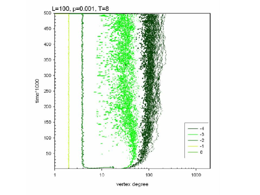
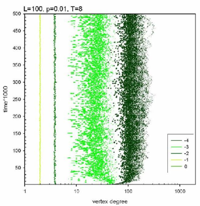
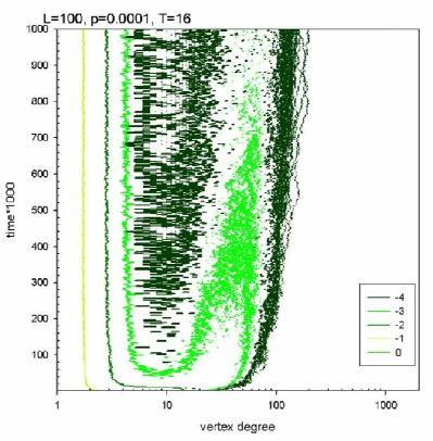
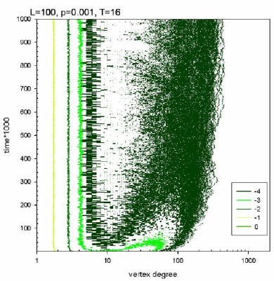
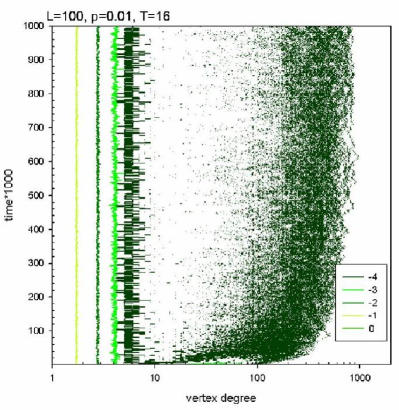
If preferences are not switched on then the network quickly reaches the stationary state with the Poisson degree distribution centered at [17]. If the preferences are switched on then for any and in a few time steps the initial degree distribution centered at transforms into some other distribution. Our focus is on the process of graph restructuring. In the series of figures: Figs 4, 5, 6 we present arguments to prove the fact that a graph evolving at any reaches a state for which further edge changes do not influence on the vertex degree distribution. Then we say that the system is self-organized into the fixed stationary state.
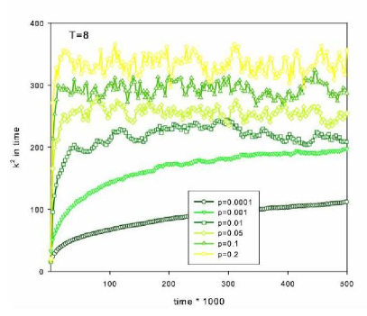
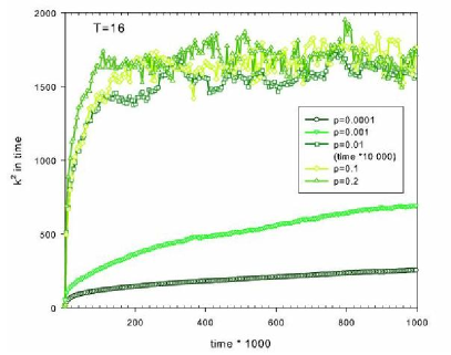
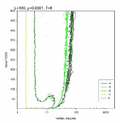
In Figs 4 and 5 typical evolutions of vertex degree distributions are presented. The horizontal axis describes vertex degree in log-scale. The vertical axis is for time steps. To quantify properties of the evolving graph, in Fig. 6 we characterize the state of the self-organization by the second moment of the distributions. The statistical physics of graphs says that graphs with a fixed number of edges compose the canonical ensemble [12, 23, 24] and the second moment (or equivalently the sum of degrees squared of all vertices) can be interpreted as the energy carried by a graph with fixed number of edges, [23, 25].
The obtained results show that changes in a graph evolving with are similar to those found for corresponding first steps of a graph evolving with . The passing time cannot be distinguished from the value of . Comparing figures with to figures with the similar observation holds. Therefore the first simulation proved fact is that rewirings in each time step after time steps is equivalent to the change made by rewiring edges in one time step for sufficiently low. In particular, the evolution with the preference threshold goes in this asynchronous way for all and the stationary state of the asynchronous evolution is reached within the observed . If then the stabilization of a system needs more time. Therefore all our observations are of time steps long. Nevertheless to reach the asynchronous dynamics ensemble in case of we let the system evolve ten times longer, so that we can state again that for all the same stationary state is observable, see legends to Fig. 6.
With increasing , namely , stationary states are reached definitely faster for both values. Here the ‘synchronized’ preferential rewiring dominates in one-step transition what results that at each the system constitutes different stationary ensemble. These ensembles are distinct quantitatively from each other by the different vertex degree distributions what reflects in the distinct values of .
3.2 Stationary state vertex distribution
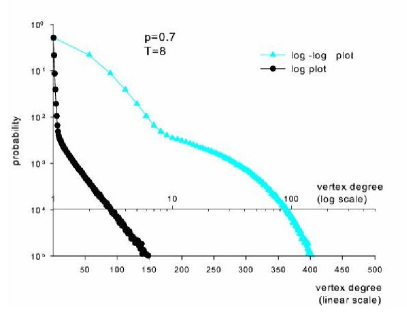
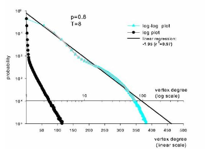
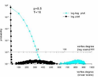
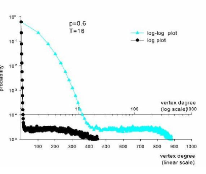
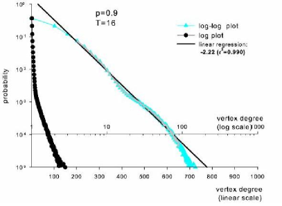
In Figs 7, 8, 9 and 10 we show distributions of the stationary states obtained at different and for and , respectively.
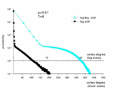
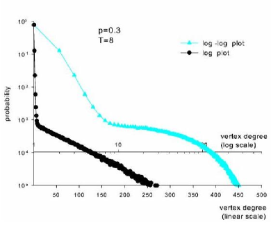
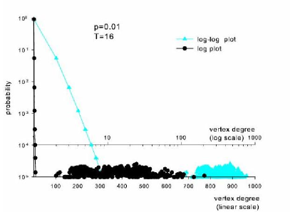

In Fig. 7 the top panel describes the graph ensemble resulting from asynchronous evolution. The degree distribution is like a two-part function. The first part represents properties of vertices which are not preferred, i.e., vertices with its degree smaller than the threshold (). The second part of the distribution represents the tail properties, i.e., probabilities to find vertices with degrees much greater than the threshold , . The tail decays exponentially with the rate (the Pearson -error is added in brackets). Between these two separated regions there is a transient region, here the transient region means , which can be described by the power-law dependence on vertex degree. The exponent for this decay is . Notice, that this transient region is not visible on the exponential curve.
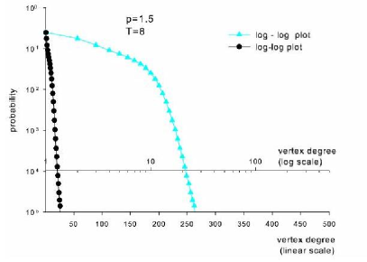
With rewiring rate increasing, the exponential tail decay slows down (at , and this is the minimal value observed by us) and then grows up to at , see the second and third panels in Fig.7. Together with fast tail decay, the transient region with power-law characteristics links to the first part of the distribution what forms the largest vertex degree interval with power-law type of distribution. At we have the exponent of the power-law decay for , see Fig. 8 top panel. However, for the decay changes into . Finally, when then the transient region vanishes. The decay corresponding to vertices with can be still approximated by a power-law but then if the fast exponential decay occurs. In particular at we have exponential rate decay and power law decay with exponent when , see Fig. 8 bottom panel.
In case the first and tail parts of degree distribution are isolated from each other for a large interval of , see the first and second panels in Fig.9. The noticeable transient region constitutes at ( for ), see Fig.9 the bottom panel. With growing , similarly to the ensembles resulting from evolution with , we observe the junction between the first and transient regions of the distribution, and the largest interval of the power-law decay establishes. Namely, when then for , see the top panel in Fig.10. However for vertices with a degree we observe the fast exponential-like decay. Stationary ensembles arising from the evolution with are similar to those described in case . The first part, which can be approximated by power-law, spreads to . Then the fast exponential decay occurs, see Fig.10.
3.3 Phase transition
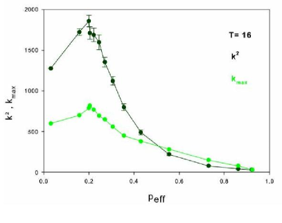
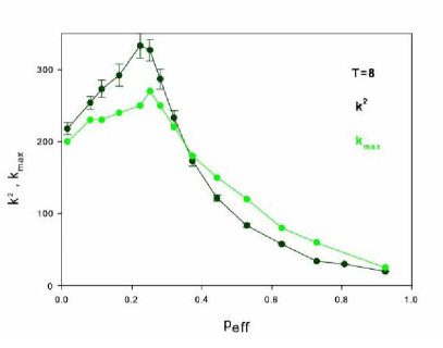
From the vertex degree distribution study it appears that at fixed there exist two different self-organized graph ensembles corresponding to the small and large value. It is said that if some global statistical property representative for a graph topology changes then such a phenomenon is referred to as topological phase transition [23]. As the most appropriate order parameters to describe this transition we consider — mean energy in the ensemble, and — the largest vertex degree which occur with probability greater than . Fig. 11 show dependences of both order parameters on . For both values and both order parameters two regions of are observed. The point of topological phase transition can be localized as
The two phases in graph topology can be described as follows:
Leafy phase:
There is a huge component consisting of almost all vertices and few little 2, 3-vertices graphs. Small number of vertices with extremely high degrees (hubs) serve as centers of this component. These centers are multiple interconnected between each other what together establishes a firm long living graph skeleton. The skeleton is close to the complete graph. Hence the strong assortativity between hubs is present. Since the vertices of the graph skeleton are surrounded by plenty of leaves then one can find the strong disassortativity between skeleton vertices and leaves. At low about 90% of vertices are leaves and therefore we call a typical network of the ensemble as leafy-complete graph and the corresponding phase as leafy phase.
Tangling phase:
At the strong expectation can arise that the network ensemble should collapse to a stochastic graph. This expectation is supported by the fact that when then there exists a degree interval, namely where the probability to unlink and probability to link to are equal to - like in a stochastic graph. Moreover, vertices with are still of high probability to be unlinked, see Fig.1.
The stochastic graph distribution is distinguished from others by the peaked shape around the average degree value, here sharp maximum at should appear. However, such distribution did not appear at any model parameters considered by us. The dynamics which persistently applies the preference rule, drives the system to other than a stochastic graph solution. There is not a typical vertex for network. Instead vertices occur with similar probability. One can think that each time step plenty of edges are moved around between the similar low degree vertices what blocks the possibility to establish vertices with higher degrees. Let us call this network ensemble as tangling net to underline activity and inefficiency of the evolution rule. The corresponding phase will be called tangling phase.
The process of transition from the leafy to tangling phase can be explained qualitatively in the following way. In leafy phase there is a pool of edges attached to vertices of little degree and a small number of vertices with high degrees which are densely interconnected between each other. The presence of multiple connections makes the skeleton connections degenerated what results in that the effective number of edges in the system is much smaller than . With growing the information about changes in the edge connections are not immediately available to other rewirings what weakens the assortativity between hubs. Therefore the graph skeleton obtains less possibility to emerge and the mechanism analogous to the preferential attachment in growing models of scale free networks [26] can occur. ‘New’ edges appear due to vanishing connection degeneracy. Though the appearance of the graph skeleton is less probable, but centers which accumulate edges occur due to the persistently applied dynamics with preferences.
4 Conclusions and discussion
By considering the network evolution as two-step: the preferential rewiring of edges and updating of the information about changes done we obtain a discrete time network evolution. In this time step scale the evolution drives a regular lattice to the graph ensemble with fixed statistical properties. The presented simulation foundings can be summarized as follows:
-
1.
Networks evolving with preferential rewiring rule self-organize into stationary states.
-
2.
The stationary states form ensembles of exponential-type networks.
-
3.
The statistical properties of the stationary states such as vertex degree distribution, its second moment and maximal vertex degree are related to model parameters and .
-
4.
In the space of stationary states two separated regions are identified:
— the limit of asynchronous preferential evolution, called leafy phase, if and
— the limit of synchronous higly rewired preferential evolution, called tangling phase, if and
Between these two phases for different model parameters the different final states occur. -
5.
The maxima of the second moment of vertex degree distribution and the largest vertex degree are localized at for both . This feature suggests that the transition point between the two phases observed can be related to this value.
-
6.
The transition goes by smashing multi-connections between vertices belonging to the graph skeleton. Since the wide interval with the power-law decay in the degree distribution is observed we can claim that the mechanizm which is characteristic for Barabasi-Albert network, namely the growth in the network [26], is present. But here this mechanizm denotes the increase in the number of effective egdes.
The two most important physical mechanisms are usually listed to explain the occurrence of power-laws [6]. (1) a rich-get-richer mechanism in which the most linked vertices get more links. Here such mechanizm is represented by the preferential attachment rule and moreover this mechanizm introduces a kind of ordering. (2)critical phenomena where the ordering mechanizm is in conflict with some dissordering process. Here, a temperature like mechanizm can be ralated to the synchronization. The synchronization weakens the order coused by the preferential rule. This confict effects in appearence of critical properties.
Rough investigations about the graph ensembles arisen when have been done but only for to limit the length of runs. Again, the limit stationary degree distributions can be divided into two classes: the leafy-complete graph ( ) and the exponential graph ( ). However, for any value of , there was not noticed a power-law dependence in the first part of the distribution as well as there was not observed any transient region. Hence, in the phase-space of parameter another topological transition can be localized.
Acknowledgment
We wish to acknowledge the support of Polish Ministry of Science and Information Technology Project: PB1472PO3200325
References
- [1] R. Albert and A.-L. Barabasi, Rev. Mod. Phys. 74, 47 (2002)
- [2] S. N. Dorogovtsev and J. F. F. Mendes, Adv. Phys. 51, 1079 (2002)
- [3] M. E. J. Newman, SIAM Review 45, 167 (2003)
- [4] Complex Networks, E. Ben-Naim, H. Frauenfelder and Z. Toroczkai (eds.), (Springer, Berlin, 2004)
- [5] D. J. Watts and S. H. Strogatz, Nature 393, 440 (1998)
- [6] M. E. J. Newman, Pareto laws, Pareto distributions and Zipf’s law, cond-mat/0412004 (2005)
- [7] M. Gitterman, J. Phys. A 33, 8373 (2000); B. J. Kim, H. Hong, P. Holme, G. S. Jeon, P. Minnhagen and M. Y. Choi, Phys. Rev. E 64, 056135 (2001); M. B. Hastings, Phys. Rev. Lett. 91, 098701 (2003)
- [8] C. P. Herrero, Phys. Rev. E 65, 0566110 (2002); C. P. Herrero, Phys. Rev. E 69, 067109 (2004)
- [9] Jian-Yang Zhu and Han Zhu, Phys.Rev.E 67 026125 (2003)
- [10] A. Aleksiejuk, J. A. Holyst and D. Stauffer, Physica A 310, 260 (2002); M. A. Sumour, M. M. Shabat and D. Stauffer, Absence of ferromagnetism in Ising model on directed Barabasi-Albert network, cond-mat/05044660
- [11] A. V. Goltsev, S. N. Dorogovtsev and J. F. F. Mendes, Phys. Rev. E 67, 026123 (2003); S. N. Dorogovtsev, A.V.Goltsev and J. F. F. Mendes, Phys. Rev. E 66, 016104 (2002)
- [12] S. N. Dorogovtsev, J. F. F. Mendes and A. N. Samukhin, Nucl. Phys. B 666, 396 (2003)
- [13] R. F. i Cancho, Ch. Janssen and R. V. Sole, Phys. Rev. E 64, 046119 (2001) M. A. Novotny and S. M. Wheeler, On The possibility of Quasi Small-World Nanomaterials, cond-mat/0308602
- [14] L. F. Lago-Fernandez, R. Huerta, F. Corbacho and J. A. Siguenza, Phys. Rev. Lett. 84, 2758 (2000)
- [15] N. Mathias and V. Gopal, Phys. Rev. E 63, 021117 (2001)
- [16] Ch. Cherniak, Trends in Neurosciences 18, 552 (1995)
- [17] D. Makowiec, in Cellular Automata, edited by P. M. B. Slot, B. Chopard and A. G. Hoestra, (Springer-Verlag, 2004), p. 141
- [18] D. Makowiec, New challenges in cellular automata due to network topology, cond-mat/0412082
- [19] D. Makowiec, Acta Phys. Pol. B (to be published)
- [20] M. E. Newman and M. Girvan, Phys. Rev. E 69, 026113 (2004)
- [21] M. E. Newman, in Complex Systems, edited by E. Ben-Naim, H. Frauenfelder and Z. Toroczkai (Springer, Berlin, 2004) p. 337
- [22] P. Erdös and A. Rényi, Math. Inst. Hung. Acad. Sci. 5, 7 (1960)
- [23] I. Farkas, I. Derenyi, G. Palla and T. Viscek, in Complex Networks edited by E. Ben-Naim, H. Frauenfelder and Z. Toroczkai, (Springer, Berlin, 2004), p.163
- [24] Z. Burda, J. D. Correia and A. Krzywicki, Phys. Rev. E 64, 046118 (2001)
- [25] J. Berg and M. Lässing, Phys. Rev. Lett. 89, 228701 (2002)
- [26] A. -L. Barabasi, R. Albert, Science 286 50, (1999)