The Topological Non-connectivity Threshold and magnetic phase transitions in classical anisotropic long-range interacting spin systems

Abstract

We analyze from the dynamical point of view the classical characteristics of the Topological Non-connectivity Threshold (TNT), recently introduced in F.Borgonovi, G.L.Celardo, M.Maianti, E.Pedersoli, J. Stat. Phys., 116, 516 (2004). This shows interesting connections among Topology, Dynamics, and Thermo-Statistics of ferro/paramagnetic phase transition in classical spin systems, due to the combined effect of anisotropy and long-range interections.

I Introduction

The magnetic properties of materials are usually described in the frame of system models, such as Heisenberg or Ising models where rigorous results, or suitable mean field approximations are available in the thermodynamical limit. On the other side, modern applications require to deal with nano-sized magnetic materials, whose intrinsic features lead, from one side to the emergence of quantum phenomenachud , and to the other to the question of applicability of statistical mechanics. Indeed, few particle systems do not usually fit in the class of systems where the powerful tools of statistical mechanics can be applied at glance. In particular, an exhaustive theory able to fill the gap between the description of $2$ and $10^{23}$ interacting particles is still missing. Moreover, also important well-established thermodynamical concepts as the temperature, become questionable at the nano-scaletempe . In a similar way, long-range interacting systems belong, since long, to the class where standard statistical mechanics cannot be applied tout court. Indeed, they display a number of bizarre behaviors, to quote but a few, negative specific heat Lynden-Bell and hence ensemble inequivalence InEq , temperature jumps, and long-time relaxation (quasi-stationary states)QSS . Therefore, from this point of view, few-body short-range interacting systems share some similarities with many-body long-range ones.

Within such a scenario, and thanks to the modern computer capabilities, it is quite natural take a different point of view, starting investigations directly from the dynamics, classical and quantum as well celardo . It was in this spirit that quite recently in a class of anisotropic Heisenberg-like spin lattice systems, a topological non-connection of the phase space was discovered jsp . Initially, for historical reasons palmer , this was referred to as broken ergodicity, since if the phase space is decomposable in two unconnected parts (hence topologically non-connected) then a breaking of the ergodicity is indeed a trivial consequence khinchin . Here we prefer to call Topological Non-connectivity Threshold (TNT) the value $E_{tnt}$ where such a disconnection sets in upon lowering the total energy $E$ of the system. This result was found, first numerically and later analytically, in a class of spin models where important and rigorous results have been obtained during the last century, though generally only in the thermodynamical limit (total number of microscopic constituents of the system $N\to\infty$ keeping fixed the number density $N/R^{d}$, where $R$ is the spatial size of the system and $d$ is its spatial embedding dimension). Nevertheless, to the best of our knowledge, apparently nobody took care of the dynamics, and consequently nobody spoke of this simple but relevant property.

This dynamical point of view has a few interesting classical consequences. First of all it explains, from the point of view of microscopic dynamics, the possibility of ferromagnetic behavior in small system. Indeed, in absence of external field and external noise (temperature) a magnetized system, (belonging to one branch of the non-connected phase space) remains magnetized simply because it cannot move to the other one. Furthermore, our TNT is surely related to recent resultspettini ; HK ; ARZ connecting topological transitions (TT) and thermo-statistical phase transitions (PT), even if such investigations again concern the thermodynamical limit only, and they relate to usual PT of canonical thermo-statistics. However, it has been recently stressed Gross that microcanonical thermo-statistics is the theoretically more suitable description for systems with small size and/or long-range interactions.

We therefore begin in Section II with a short description of our class of models and the topological properties of the TNT for finite and infinite $N$, pointing out the crucial role played by the first key ingredient of our models, the $XY$ anisotropy In particular we would like to answer the following question: what happen to the energy $E_{tnt}$ and to the corresponding $N$-spin configuration $\vec{S}_{tnt}^{N}$ when the $N\to\infty$? It is exactly answering this question that the deep connection between TNT and the other key ingredient, the long-range interactions, becomes apparent. Our results brescia can be summarized as follows:

1) For finite sized systems TNT exists for short range and long range as well, as soon as anisotropy persists.

2) When the number of particles becomes large the energy size of the non-connected region goes to zero with respect to the total energy size for short range interaction while it goes to some finite quantity for long range ones.

In Section III we switch to the dynamical properties found in firenze which accompany such a special (and rather “big”) TT, and its relations with its thermostatistical properties, namely the occurence and location of a usual (paramagnetic/ferromagnetic) PT, using techniques from large deviation theory dauxois within the microcanonical description of the system.

We conclude in IV. Everywhere here we restrict ourselves to the classical case; for a recent discussion of its quantum counterpart, we refer to bcb ; bct .

II Mechanics and Topology

As a paradigmatic model example of TNT, let us consider the following class of lattice spin models, described by the Heisenberg-like Hamiltonian:

$$H={\eta\over 2}\sum_{i\not=j}^{N}{S^{x}_{i}S^{x}_{j}\over r_{ij}^{\alpha}}-{1\over 2}\sum_{i\not=j}^{N}{S^{y}_{i}S^{y}_{j}\over r_{ij}^{\alpha}}$$ (1)

where $S^{x}_{i},S^{y}_{i},S^{z}_{i}$ are the spin components, assumed to vary continuously; $i,j=1,...N$ label the spins positions on a suitable lattice of spatial dimension $d$, and $r_{ij}$ is the inter-spin spatial separation therein. Here for simplicity we consider a $d=1$ lattice. (See brescia for extensions to $d=2,3$.) For later notational convenience, we define the single-spin vector $\vec{S}=(S^{x}_{i},S^{y}_{i},S^{z}_{i})$ and the $N$-spin configuration $\vec{S}^{N}=(\vec{S}_{1},\vec{S}_{2},...\vec{S}_{N})$. The tip of each $i$-th spin is taken to lie on the unit sphere, i.e. it satisfies the constraint $(S^{x}_{i})^{2}+(S^{y}_{i})^{2}+(S^{z}_{i})^{2}=1$. Also, $\alpha>0$ parametrizes the range of interactions (decreasing range for increasing $\alpha$) and $0<\eta<1$ parametrizes the $XY$ anisotropy. For $\alpha=\infty$ we recover nearest-neighbor interactions, while $\alpha=0$ corresponds to infinite-range interactions. A mean-field model is obtained by setting $\alpha=0$ and including as well the (somewhat non-physical) self-interaction pairs $i=j$:

$$H_{mf}=\frac{\eta}{2}N^{2}(m_{x})^{2}-\frac{1}{2}N^{2}(m_{y})^{2},$$ (2)

where $m_{x,y,z}=(1/N)\sum_{i}^{N}S^{x,y,z}_{i}.$ While this might be thought of as a negligible modification for $N\to\infty$, nevertheless it has non-negligible effects concerning the chaoticity properties of the system. Indeed, the dynamics of the truly mean-field $\alpha=0$ system turns out to be exactly integrablefirenze . Here we are not interested in the most general spin Hamiltonian giving rise to a TNT (for instance in jsp ; firenze a term containing a transversal magnetic field $B_{z}$ has been added to $H$). Rather, we focus on the very simple Hamiltonian (1) which already contains the two essential ingredients which give rise to the TNT, i.e. anisotropy and long-range, whose main effects are conveniently encapsulated within two simple and easy-to-handle parameters $\alpha$ and $\eta$, in order to make the study of the minimum-energy configurations analytically tractable at $N\to\infty$ and numerically feasible at finite $N$. Concerning the physical motivations for such choices, we refer to the recent discussion in bct .

Depending on the specific $N$-spin configuration the corresponding energy $E=H(\vec{S}^{N})$ will vary according to (1). One (not necessarily unique) configuration $\vec{S}^{N}_{min}$, to be specified soon, turns out to have minimum energy $E_{min}$, defined by the minimum of the Hamiltonian (1) over all conceivable configurations:

$$E_{min}=Min\ [\ H\ ]\ .$$ (3)

Since $0<\eta<1$ the minimum energy configuration $\vec{S}^{N}_{min}$ is attained when all spins are aligned along the $Y$ axis, which defines implicitly the easy axis of magnetization. In the same way, let us define the TNT energy $E_{tnt}$ as the minimum energy compatible with the constraint of zero magnetization along the easy axis of magnetization:

$$E_{tnt}=Min\ \left[\ H\ \left|\ m_{y}=0\ \right]\right..$$ (4)

corresponding to some other $N$-spin configuration $\vec{S}^{N}_{tnt}$ to be specified later. By definition, in general $E_{min}\leq E_{tnt}$, and in particular it may be that $E_{min}\neq E_{tnt}$. We call this situation is topological non-connection, as will become clear in a moment, and its physical (dynamical as well as statistical) consequences are rather interesting. Indeed, consider a system prepared at time $t=0$ with a definite sign of magnetization, say $m_{y}>0$ and an energy value $E_{min}\leq E\leq E_{tnt}$. As time goes by, the system evolves upon the constant energy surface $H(\vec{S}^{N})=E$ in configuration space. Nevertheless, due to the continuity of the dynamical equations of motion the magnetization $m_{y}(t)$ (not a constant of motion) may well change its size, but it can never change its sign, instead. Indeed, in order to assume a value $m_{y}<0$ it should have to go through at least one configuration with $m_{y}=0$, which by definition cannot belong to the $E<E_{tnt}$ surface. The whole situation can be summarized as follows.

Topology: in configuration space the surface at fixed energy $E$ is topologically non-connected in two components, each characterized by a magnetization either $m_{y}<0$ or $m_{y}>0$.

Dynamics: though the two components are energetically accessible on equal grounds, the ergodicity of the constant $E$ surface is trivially broken, since there exist no dynamically allowed path inbetween them.

Thermo-Statistics: de-magnetization is in principle impossible below the TNT, so we may speak in some sense of a ferromagnetic phase. Of course, the application of a magnetic field, or a thermal noise, can give the energy necessary to overcome the energy barrier, thus in principle - if not in practice - allowing for a magnetic reversal. On the contrary, for energy values $E>E_{tnt}$, de-magnetization is in principle possible, and we may speak in some sense of a paramagnetic phase. However, being above the TNT does not automatically guarantee that, for any combination of parameter values and initial conditions, a system initially magnetized at $t=0$ will for sure eventually de-magnetize within a given finite observational time $t_{obs}$. First, as reported in firenze some invariant multidimensional structures can appear in phase-space preventing the motion from covering the whole energy surface. This lack of ergodicity is well known in 2D Hamiltonian systems, where KAM tori prevent motion from wandering the whole phase space chirikov , while it turns out to be more complicated in multidimensional system, see for instance the famous Fermi-Pasta-Ulam problem (for interesting reviews see ford ; felix ). Such invariant structures usually disappear in the presence of strongly chaotic motions chirikov . We can therefore say that strong chaos is somehow another necessary ingredient in order for the system to be in its paramagnetic phase. Second, even given strong enough chaoticity to “encourage” the system to explore all the available phase (or configuration) space, yet the system could be given not enough time to actually do it, so effectively “freezing” it within the $m_{y}$ component where it started from.

For finite $N$ systems the $XY$ anisotropy is the only necessary ingredient in order to have $E_{tnt}<E_{min}$ and hence the TNT. For $N\to\infty$, one quickly realizes that $E_{min}\to-\infty$ and guesses that $E_{tnt}\to-\infty$, but may still wonder wehther $E_{tnt}\to E_{min}$ as well, thus making the TNT physically irrelevant. So we define the topological non-connection ratio:

$$r=\frac{E_{tnt}-E_{min}}{|E_{min}|},$$ (5)

which expresses how large a fraction of the energy range is topologically non-connected. Here we use the denominator $E_{min}$ (instead of the whole energy range), since, in such kind of models, one is usually interested in the negative energy range only. Correspondingly, we will refer to a system as topologically non-connected if $r\to const\neq\ 0$ in the limit $N\to\infty$.

To show why and how this whole comes by in our models, we now concentrate on the energy $E$ of the above mentioned interesting $N$-spin configurations. The minimum-energy configuration $\vec{S}^{N}_{min}$ (all spins aligned along the $Y$-axis), can also be thought of as composed of $2$ equal blocks of $N/2$ spins, all up. Correspondingly, the minimum energy $E_{min}<0$ can be split into 3 contributions, namely $2$ equal intra-block bulk energies $E_{\uparrow}<0$ plus $1$ inter-block interaction energy $V_{\uparrow\uparrow}<0$. Flipping just 1 block, its bulk energy does not change, i.e. $E_{\uparrow}=E_{\downarrow}<0$, but the interaction energy reverses sign to $V_{\uparrow\downarrow}=-V_{\uparrow\uparrow}>0$. However, in such a new configuration $\vec{S}^{N}_{\uparrow\downarrow}$ the magnetization is now $m_{y}=0$. Both bulk energies are as low as they can, while the constraint $m_{y}=0$ frustrates the total energy to rise above $E_{min}$ by an amount $2|V_{\uparrow\uparrow}|$. We therefore take $E_{\uparrow\downarrow}=E_{min}+2|V_{\uparrow\uparrow}|$ as a somewhat obvious candidate for $E_{tnt}$ and the related spin configuration $\vec{S}^{N}_{\uparrow\downarrow}$ as the TNT spin configuration $\vec{S}^{N}_{tnt}$.

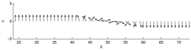
Figure 1: TNT spin configuration. Here is $\alpha=0.1$, $N=100$, $\eta=0.9$. Only the central part of the chain has been shown.

A $d=1$ example of a numerically obtained $\vec{S}^{N}_{\uparrow\downarrow}$ is given in Fig. 1. As one can see, excluding a small central domain, the spins are arranged in two equal-size blocks with opposite spins, i.e. the real $\vec{S}^{N}_{tnt}$ is remarkably similar to, though in fact somewhat slightly different from, the ideal $\vec{S}^{N}_{\uparrow\downarrow}$. Extensive numerical simulations using constrained optimization and analytical estimates as wellbrescia , confirm such an impression, with natural analogues in $d=2,3$.

Quite generally, the exact TNT configuration at finite $N$ for arbitrary $\alpha$ and $\eta$ can be found only numerically. Nevertheless, concerning the large $N$ limit it is possible to make a few definite statements brescia . First, if $\alpha\neq 0$, $\eta=\-1$, and $N$ sufficiently large, then $\vec{S}^{N}_{\uparrow\downarrow}\simeq\vec{S}^{N}_{\uparrow\downarrow}$, in the twofold sense that the TNT spin configuration is approximately half up and half down, and the energy difference $E_{dom}:=E_{tnt}-E_{\uparrow\downarrow}$ due to the domain is a finite quantity independent of $N$. Second, for $N\to\infty$, if $\alpha>d$ (short-range) then $r\to 0$ but if $\alpha<d$ (long-range) then $r\to const\neq 0$. In particular, if $d=1$ then $r_{\infty}=2-2^{\alpha}$. Intuitively, while for short-range the bulk volume contribution $E_{\uparrow}+E_{\downarrow}$ eventually dominates over the geometric inte(sur)face area energy interaction $V_{\uparrow\uparrow}0$, for long-range interactions the “effective interface” is the whole bulk as well. As now both the inter-block and the intra-block interaction involve all spin pairs in the two blocks, though each pair with a different intensity $\propto r_{ij}^{-\alpha}$, energies will then scale like the number of pairs $\propto N^{2}$ times the interaction at typical distance $r_{ij}\simeq R$. So there holds the same scaling $|V_{\uparrow\uparrow}|\sim(R^{d})^{2}/R^{\alpha}\sim N^{2-\alpha/d}\sim|E_{min}|$, though with different (and $\alpha$-dependent) proportionality constants, and so $r\simeq const\not\to 0$ as $N\to\infty$.

III Dynamics and Thermo-Statistics

Here, we show how to impose a self-consistent Hamiltonian dynamical evolution upon the spin systems described by (1). Afterward, we will employ such dynamical equations, numerically integrated for long enough times, to study the time-evolution of $\vec{S}^{N}(t)$. Following brescia ; firenze here we focus on the time evolution instantaneous magnetization $m_{y}(t)$ started with some $E$ and $m_{y}(0)$ and evolved according to (III). Complementarily, we look at its statistical distribution $P_{ens}(E,m_{y})$, built via a random sampling of an ensemble of initial conditions, all with the same $E$, tunable at will. Finally, we will show a connection between Dynamics and Thermo-Statistics.

For each $i$ the spin components $S^{x}_{i},S^{y}_{i},S^{z}_{i}$ satisfy the usual commutation rules for angular momenta, i.e. $\{S^{x}_{i},S^{y}_{j}\}=\delta_{ij}S^{z}_{i}$, (and cyclic) where $\{,\}$ are the canonical Poisson brackets. As usual, (and this procedure immediately translates to the quantum case bcb ; bct ), starting from the Hamiltonian (1) we straightforwardly derive the dynamical equations as:

$$\frac{d\vec{S}_{i}}{dt}=\{H,\vec{S}_{i}\}$$

As is well-known, for such dynamical equations the total energy $E$ and the spin moduli $|\vec{S}_{i}|^{2}=1$ are constants of the motion. Usually, for energies $E$ not too close to $E_{min}$, the dynamics is characterized by a positive largest Lyapunov exponent, corresponding to strongly chaotic motion jsp . On the contrary, the dynamics of the truly (all pairs $ij$) mean-field $\alpha=0$ system turns out to be exactly integrablefirenze . Given strong enough chaoticity, typical examples of evolution curves of $m_{y}(t)$ and corresponding $P_{ens}(E,m_{y})$, are shown in Fig. 2.

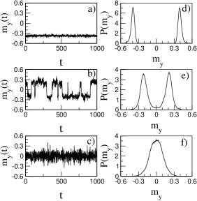
Figure 2: Left column (a,b,c) : time evolution of the magnetization $m_{y}(t)$ for different specific energy values. Right column (d,e,f) : probability distribution of the magnetization at a given specific energy. Parameters are $\alpha=0$, $\eta=1$, $N=10$. Upper line ((a,d) below the TNT ) : $E/N=-0.7$. Middle line ((b,e) between the TNT and the statistical thresholds $E/N=-0.3$. Lower line ((c,f) above the statistical threshold) $E/N=0.1$.

Again, the whole situation can be summarized as follows.

Thermo-Statistics: for $E<E_{tnt}$ (Fig. 2d) the two peaks of the distribution are well separated, while for $E>E_{tnt}$ (Fig. 2e) they come close. At $E_{stat}$ they merge into one single peak (Fig. 2f), as expected from the statistical analytical estimate. Note that this simple (and, in its roots, purely geometrical) argument immediately prooves that, in general, $E_{tnt}<E_{stat}$: excluding catastrophic situations, upon increasing $E$ the two separated inner tails must first touch at $E_{tnt}$ before the relatively outer twin peaks may eventually merge at $E_{stat}$. Indeed, this very same argument automatically applies to any model with probability distribution changing from single to double-peaked , e.g. the discrete mean field $\varphi^{4}$ model HK . In other words, if both a TNT and a PT are known to exist, then in general they will occur at different energies. And depending on wether $E$ is increased or decreased, both a TNT and a PT in some sense “anticipate” each other. Of course, for a given specific system nothing automatically guarantees that either a TNT or a PT do indeed both exist. So, while in principle a TNT and a PT neither imply nor exclude each other, in practice they “strongly suggest” each other.

Dynamics: at low energy (a) the system is always magnetized with small fluctuations, and at high energy (b) the system is on average non-magnetized with large fluctuations. In between (c) the magnetization jumps erratically up and down. We can usefully define a magnetic-reversal time-scale firenze , as the average time necessary to magnetization to reverse its sign. In the presence of strong chaos (dependent on the parameters $N$ and $E$) magnetic reversals occur fully at random, with the distribution of jumping times following a Poisson distribution. Any deviation from such distribution, for large $N$ and large negative $E$ values, signals the presence of invariant curves preventing the motion to switch from one peak to the other one.

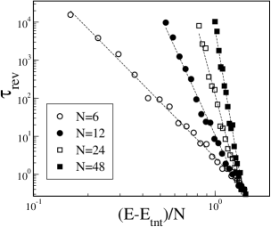
Figure 3: Divergence of magnetization reversal times close to the TNT. Here is $\alpha=0$, $\eta=1$, and different $N$ values as indicated in the insert. Lines are the best fit according to Eq. (6).

Interestingly, and somewhat reminiscent of a critical PT, as shown in Fig. 3 the magnetic-reversal time-scale diverges as a power law of $E$ at the critical energy $E_{tnt}$:

$$\tau_{rev}\sim\left[{E-E_{tnt}\over N}\right]^{-\gamma(N)}$$ (6)

where $\gamma(N)\propto N$.

Remarkably, such a dynamical behavior can be qualitatively - and almost quantitatively - explained only by statistical considerations. Before that, let us remark that (6) can be inverted for $E$ at any fixed $N$, thus giving a $\tau$-depending characteristic energy $E_{rev}(\tau)$. We will see the physical meaning of $E_{rev}$ in a while; here we just note that, since (6) holds only for $E>E_{tnt}$, it will also be $E_{rev}>E_{tnt}$.

Thermo-Statistics: restricting attention to the mean field Hamiltonian (2), a detailed statistical analysis using techniques from large deviations theory leads to definite predictions (see firenze for details) concerning the microcanonical (i.e., purely state-counting at fixed $E$) probability distribution $P_{stat}(m_{y},E)$, the topological energy threshold $E_{tnt}$, and the thermo-statistical energy threshold $E_{stat}$, where the system undergoes a continuous ferro/paramagnetic PT in the microcanonical description.

Dynamics: Adopting a viewpoint as close as possible to the experimental one, we introduce an observational time $t_{obs}$, during which the experiment can be performed. Assuming the experimentally measured value and the dynamically observed time-average to coincide, we introduce the $t_{obs}$-averaged magnetization:

$$\langle m_{y}\rangle=\int_{0}^{t_{obs}}\ dt\ m_{y}(t).$$ (7)

The quantity $\langle m_{y}\rangle$ as a function of the energy $E$ can be compared with $\hat{m}_{y}(E)$, obtained from the most likely values $P_{stat}(E,\hat{m}_{y})$ (the maxima of the distribution). This is shown in Fig. 4, where we have also indicated the thresholds $E_{stat}$ and $E_{tnt}$ as vertical lines.

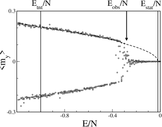
Figure 4: Numerical $t_{obs}$-averaged dynamical magnetization as a function of the specific energy $\epsilon=E/N$ (circles). Dashed line are the analytical predictions from the thermo-statistical mean field model (2). Here is $N=60$, $\alpha=0$, $\eta=1$. For the sake of comparison, both the thermo-statistical phase transition and the topological non-connectivity thresholds have been indicated as vertical lines. Also indicated, as a vertical arrow, the expected dynamical magnetic-reversal threshold.

Of course, below $E_{tnt}$ and above $E_{stat}$ the two averages coincides, at variance with the region between them. Also, the effective transition given by $\langle m_{y}\rangle$ occurs at some intermediate energy, different from both $E_{tnt}$ and $E_{stat}$. This is not completely surprising, since both the topological energy $E_{tnt}$ and the thermo-statistical energy $E_{stat}$ refer to some limiting properties, the former when $t\to\infty$ at any finite $N$, the latter when $N\to\infty$ at any time $t$. It is interesting to note that, inverting Eq. (6), to the observation time $t_{obs}$ there correspond a dynamical energy $E_{rev}(t_{obs})$ which is in fairly good agreement with the observed transition energy, see Fig. 4.

Note also that, to a rather good accuracy firenze ; bcb , there holds the following proportionality between the dynamical quantity $\tau_{rev}$ and the statistical quantity $P(E,m_{y})$:

$$\tau_{rev}\propto{\hat{P}\over P_{0}}$$ (8)

where $\hat{P}=P_{stat}(E,\hat{m}_{y})$ and $P_{0}=P_{stat}(E,0)$. Theoretically firenze , this can be traced back to the occurence of an entropy barrier $\Delta S:=\hat{S}-S_{0}$ between the two components, where $\hat{S}=\ln\hat{P}$ and $S_{0}=\ln P_{0}$, under the assumption of markovicity of the dynamical evolution. Detailed statistical consideration on the mean field model (2) lead to the analytical estimate $\gamma_{stat}(N)=N$ to be compared with the numerical result $\gamma_{stat}(N)\approx 0.88N$.

Heuristically, (8) can be understood as follows. Suppose the dynamics is strongly enough chaotic, making the system almost freely wander through configuration space, in some sort of diffusive fashion. Then, the probability to encounter a configuration with $m_{y}=0$, and therefore presumably switch from the $m_{y}>0$ to the the $m_{y}<0$ component, can be assumed to be simply proportional to the ratio of the number $M_{0}$ of “right” configurations at $m_{y}=0$ to the number $M_{+}$ of “wrong” configurations at $m_{y}\neq 0$, but counting only a half of the total wrong ones, namely those on the side where the system is coming from. (The system cannot know nothing yet about the other side still it’s going to.) However, as long as the magnetization peaks are high and narrow, essentially all the “wrong” configuration are actually within the peak itself, i.e. normalizing by the total number $M=M_{+}+M_{0}+M_{-}$ of energetically allowed configurations gives the probabilities $P_{+}\simeq\hat{P}$. Finally, the average time needed for magnetic reversal can be assumed to be taken proportional to the probability to encounter the right configuration with $m_{y}=0$, times some characteristic “residence time” $\tau_{res}$ during which the system essentially stays within each given $N$-spin configuration, along its longer wandering of the whole $N$-spin configuration space. Altogether, such a purely statistical argument recovers exactly (8), implicitly suggesting that the precise value of $\tau_{res}$ might be the origin of the different coefficients found between the classical firenze and quantum bcb realizations of the same dynamical evolution equations (III).

IV Conclusions

We showed the existence in classical Heisenberg spin models of a Topological Non-connectivity Threshold (TNT), caused by the anisotropy of the coupling when it induces an easy-axis of the magnetization. Below the TNT the constant energy surface is topologically disconnected in two symmetrically equal components.

Such a result on the Topology has connections both with the Dynamics (time-scales) and with the Thermo-Statistics (PT) of the system. In each component the magnetization along the easy axis has a definite sign, and it cannot change sign as time goes by, corresponding a ferromagnetic behavior of the system. Above the TNT, in a strong chaotic regime, the magnetization reverses its sign with a characteristic time-scale which diverges as a power law at the TNT. Given enough chaos and enough observational time, this leads to a paramagnetic behavior of the system. Moreover, the numerically observed link between time-scales and probability distributions has been given an heuristical justification.

The connection between the TNT and the range of the interaction has also been shown. For macroscopic spin systems the existence of this threshold determines a disconnected energy range that remains relevant (w.r.t. the total energy range) for long-range interactions, while it goes to zero for short-range interactions.

References

- (1) E. M. Chudnovsky and J. Tejada, Macroscopic Quantum Tunneling of the Magnetic Moment, Cambridge University Press, (1998).
- (2) M. Hartmann, G. Mahler and O. Wess. Phys. Rev. Lett. 93, 80402 (2004).
- (3) D.Lynden-Bell, R.Wood, Mon. Not. R. Astr. Soc. 136, 101 (1967); W.Thirring, Z. Phys. 235, 339 (1970); D.Lynden-Bell, R.M.Lynden-Bell, Mon. Not. R. Astr. Soc. 181, 405 (1977); D.Lynden-Bell, cond-mat/9812172.
- (4) J. Barré, D. Mukamel, S. Ruffo, Phys. Rev. Lett. 87, 3, (2001).
- (5) J. Barré, F. Bouchet, T. Dauxois, and S. Ruffo, Phys. Rev. Lett. 89, 110601, (2002)
- (6) R. G. Palmer, Adv. in Phys., 31, 669 (1982).
- (7) A. I. Khinchin Mathematical Foundations of Statistical Mechanics, Dover Publications, New York (1949).
- (8) L.Caiani, L.Casetti, C.Clementi, M.Pettini, Phys. Rev. Lett. 79, 4361 (1997); L.Casetti, M.Pettini, E.G.D.Cohen, Phys. Rept. 337, 237 (2000); L.Casetti, M.Pettini, E.G.D.Cohen, J.Stat.Phys. 111, 1091 (2003); R.Franzosi, M.Pettini, Phys. Rev. Lett. 92, 060601 (2004); R.Franzosi, M.Pettini, L.Spinelli, cond-mat/05005057. R.Franzosi, M.Pettini, cond-mat/05005058.
- (9) M.Kastner, Phys. Rev. Lett. 93, 150601 (2004); I.Hahn, M.Kastner, cond-mat/0506649; I.Hahn, cond-mat/0509136; M.Kastner, cond-mat/0509206.
- (10) L.Angelani, G.Ruocco, F.Zamponi, Phys. Rev. E 72, 016122 (2005).
- (11) D.H.E.Gross, Phys.Rept.279, 119 (1997); D.H.E. Gross Microcanonical Thermodynamics: Phase Transitions in Small Systems, Lecture Notes in Physics 66, World Scientific, Singapore, 2001;
- (12) G. L. Celardo, PhD dissertation, University of Milano, Italy (2004).
- (13) F. Borgonovi, G. L. Celardo, M. Maianti, E. Pedersoli, J. Stat. Phys., 116, 516 (2004).
- (14) F. Borgonovi, G.L. Celardo, A. Musesti, and R. Trasarti-Battistoni cond-mat/0505209.
- (15) G.L.Celardo, J.Barré, F.Borgonovi, S. Ruffo, cond-mat/04010119.
- (16) T. Dauxois, S. Ruffo, E. Arimondo, M. Wilkens Eds.,Lect. Notes in Phys., 602, Springer (2002).
- (17) F. Borgonovi, G. L. Celardo, and G. P. Berman, cond-mat/0506233.
- (18) F. Borgonovi, G. L. Celardo, and R. Trasarti-Battistoni cond-mat/0510079
- (19) B. V. Chirikov Phys. Rep., 52, 253 (1979).
- (20) J. Ford, , Phys. Rep. 213, 271 (1992).
- (21) G. P. Berman and F. M. Izrailev, Chaos 15, 015104 (2005).