Occurrence of normal and anomalous diffusion in polygonal billiard channels

Abstract

From extensive numerical simulations, we find that periodic polygonal billiard channels with angles which are irrational multiples of $\pi$ generically exhibit normal diffusion (linear growth of the mean squared displacement) when they have a finite horizon, i.e. when no particle can travel arbitrarily far without colliding. For the infinite horizon case we present numerical tests showing that the mean squared displacement instead grows asymptotically as $t\log t$. When the unit cell contains accessible parallel scatterers, however, we always find anomalous super-diffusion, i.e. power-law growth with an exponent larger than $1$. This behavior cannot be accounted for quantitatively by a simple continuous-time random walk model. Instead, we argue that anomalous diffusion correlates with the existence of families of propagating periodic orbits. Finally we show that when a configuration with parallel scatterers is approached there is a crossover from normal to anomalous diffusion, with the diffusion coefficient exhibiting a power-law divergence.

I Introduction

Billiard models, in which point particles in free motion undergo elastic collisions with fixed obstacles, have simple microscopic dynamics but strong ‘statistical’ behavior, such as diffusion, at the macroscopic level. The statistical properties of scattering billiards such as the Lorentz gas, which have smooth, convex scatterers, are well-understood: see e.g. Szász (2000) for a collection of reviews. Recently, however, models with polygonal scatterers have attracted attention, since they are only weakly chaotic, with for example all Lyapunov exponents being $0$, but they still exhibit surprising statistical properties in numerical experiments Dettmann and Cohen (2001); Alonso et al. (2002); Li et al. (2003).

The dynamics in polygonal billiards depends strongly on the angles of the billiard table. Some rigorous results are available for angles which are all rational, i.e. rational multiples of $\pi$: see Gutkin (2003) and references therein. In particular, an initial condition with a given angle cannot explore the whole phase space, since the possible angles obtained in the resulting trajectory are restricted, so that the model does not have good ergodic properties. Previous numerical work has shown that if one angle is rational and the others irrational, then the results are sensitive to the value of the rational angle Alonso et al. (2002); Li et al. (2003).

In this work we restrict our attention to the case in which all angles are irrational multiples of $\pi$. There are few rigorous results available in this case, but there is numerical evidence that the dynamics is mixing in irrational triangles Casati and Prosen (1999).

We have performed extensive simulations of the transport properties of quasi-one-dimensional polygonal channel billiards; here we report detailed results for two classes of model. In both we find that transport generically corresponds to what is usually referred to as normal diffusion, i.e. linear growth of the mean squared displacement, when the particles cannot travel arbitrarily long distances without collisions (finite horizon). By ‘generic’ we mean that the set of models which do not exhibit normal diffusion is ‘small’, for example having measure zero in the space of geometrical parameters. Similarly, for the infinite horizon case we find that transport is generically marginally super-diffusive, i.e. there is a logarithmic correction to the linear growth law of the mean squared displacement.

However, we also find exceptions to the generic behaviors described above. These exceptions occur when there are parallel scatterers in the unit cell which are accessible from one another (see Sec. III for the definition). In such cases we always find super-diffusion, i.e. the mean squared displacement grows like a power law with exponent greater than $1$. Further, we demonstrate that as a parallel configuration is approached, the transition from normal to anomalous diffusion occurs through a power-law divergence of the diffusion coefficient. We also show that the exponents we obtain are not consistent with a simple continuous-time random walk model of anomalous diffusion.

Our results are consistent with previous observations of irrational models exhibiting normal Alonso et al. (2002, 2004); Li et al. (2003) and anomalous Zaslavsky and Edelman (1997); Zaslavsky (2002); Li et al. (2002); Prosen and Znidaric (2001) diffusion. Also, very recently, numerical results corresponding to one of the models studied in this work were reported in Jepps and Rondoni (2006), where it was also observed that parallel scatterers result in anomalous diffusion; the results we obtain complement and extend those of that reference.

Energy transport in polygonal billiards placed between two heat reservoirs at different temperatures has also been a focus of attention Alonso et al. (2002, 2004); Li et al. (2003). This process is closer to “color diffusion” than to heat conduction due to the absence of particle interactions and, hence, of local thermodynamic equilibrium Dhar and Dhar (1999). In these systems the properties of the energy transport process are known to be closely related to those of the particle diffusion process Li and Wang (2003); Denisov et al. (2003), and for this reason we only study the latter.

I.1 Models

The unit cells of our models are shown in Fig. 1; the complete channel consists of an infinite horizontal periodic repetition of such cells. The polygonal Lorentz model is a polygonal channel version of the Lorentz gas channel studied in Sanders (2005), consisting of a quasi-1D channel with an extra square scatterer at the center of each unit cell. By quasi-1D we mean that particles are confined to a strip infinitely extended in the $x$-direction but of bounded height in the $y$-direction.

The polygonal Lorentz model can be simplified by eliminating the central scatterer and flipping the bottom line of scatterers to point upwards, resulting in the quasi-1D zigzag model. Both models are designed to permit a finite horizon by blocking all infinite corridors in the structure, so that there is an upper bound on the distance a particle can travel without colliding with a scatterer; in scattering billiards this condition was shown to be necessary for normal diffusion to occur Bunimovich et al. (1991); Bleher (1992). The zigzag model has also been studied in Jepps and Rondoni (2006).

We remark that the zigzag model with parallel sides can be reduced to a parallelogram with irrational angles. This simple billiard geometry seems to have been neglected previously, although it is close to a model considered in Kaplan and Heller (1998) which was reported to exhibit a very slow exploration of phase space. We have found similar behavior in the parallel zigzag model (see also Jepps and Rondoni (2006)), but it appears to be a peculiarity of this model which is not necessarily shared by other polygonal billiards exhibiting anomalous diffusion.

Figure 1: Unit cells of (a) the polygonal Lorentz model, and (b) the zigzag model.

I.2 Simulations

In our simulations we distribute $N=10^{7}$ initial conditions (unless otherwise stated) uniformly with respect to Liouville measure, i.e. with positions distributed uniformly in the available space in one unit cell, and velocities with unit speed and uniformly distributed angles. We consider only irrational angles for the billiard walls in each model, although we vary explicitly scatterer heights rather than angles, and to fix the length scale we take $d=1$ (see Fig. 1) .

We study statistical properties of the particle positions $x(t)$ as a function of time $t$, denoting averages at time $t$ over all initial conditions by $\langle\cdot\rangle_{t}$. Of particular interest is the mean squared displacement $\langle\Delta x^{2}\rangle_{t}$, where $\Delta x_{t}:=x(t)-x(0)$, which is frequently used to characterize the transport properties of such systems.

II Normal and marginally anomalous diffusion

In this paper, by normal diffusion we mean asymptotic linear growth of the mean squared displacement $\langle\Delta x^{2}\rangle_{t}$ as a function of time $t$, which we denote by $\langle\Delta x^{2}\rangle_{t}\sim t$ as $t\to\infty$. This is characteristic of systems commonly thought of as ‘diffusive’, for example random walkers which take uncorrelated steps of finite mean squared length.

Strongly chaotic dynamical systems, such as the Lorentz gas, are known to exhibit normal diffusive behavior Szász (2000); this arises due to a fast decay of correlations, even between neighboring trajectories, so that after a short correlation time the dynamics looks ‘random’. It is rather surprising, then, that normal diffusion also seems to appear in non-chaotic polygonal billiards Alonso et al. (2002, 2004); Li et al. (2003) in which correlations do not decay exponentially. In these systems, the only source of ‘randomization’ arises due to divergence of neighboring trajectories colliding on different sides of a corner of the billiard: see e.g. van Beijeren (2004) for a recent attempt to characterise this randomization effect.

In the following, we present sensitive tests which provide strong confirmation that, apart from exceptional cases, the decorrelation induced by the randomization mechanism mentioned above is indeed sufficient to give rise to normal diffusion in polygonal billiards. In particular our tests distinguish the logarithmic correction (marginally anomalous diffusion) which arises generically in these systems when they have infinite horizon, as it does in fully chaotic billiards.

We will see that exceptions to these behaviors occur when the billiards present accesible parallel walls. In such cases we argue that long time correlations persist, related to the existence of families of travelling periodic orbits, which always give rise to anomalous diffusion.

II.1 Growth of second moment

The growth of the mean squared displacement $\langle\Delta x^{2}\rangle_{t}$ as a function of time $t$ is the most commonly used indicator of transport properties. In Fig. 2 we plot $\langle\Delta x^{2}\rangle_{t}$ for several non-parallel zigzag models, varying $h_{1}$. For values of $h_{1}$ below $h_{3}=0.45$ there is a finite horizon and we find that a linear regime is rapidly attained, suggesting normal diffusion. For values of $h_{1}$ above this value, there is an infinite horizon; in this case, the mean squared displacement is still almost linear, although a small amount of curvature is visible.

Figure 2: (Color online) $\langle\Delta x^{2}\rangle_{t}$ as a function of $t$ in the zigzag model with $h_{2}=0.77$ and $h_{3}=0.45$. There is a finite horizon only when $h_{1}\leq h_{3}=0.45$; curvature is barely visible in the infinite horizon cases. Statistical errors are smaller than the line width.

Normal diffusion corresponds to an asymptotic slope $1$ of $\langle\Delta x^{2}\rangle_{t}$ on a double logarithmic plot. Figure 3 shows such a plot for the same data as in Fig. 2, and we see that indeed the slope is $1$ for finite horizon and close to $1$ for infinite horizon (e.g. slope $1.06$ for $h=0.71$). For models with irrational angles and no accessible parallel sides (see Sec. III), we always find a growth exponent close to $1$, so that normal diffusion is generic in polygonal billiard channels.

Figure 3: (Color online) $\langle\Delta x^{2}\rangle_{t}$ as a function of $t$ on a double logarithmic plot in the zigzag model with the same parameters as in Fig. 2.

The above test does not, however, take account of logarithmic corrections such as those found in the Lorentz gas with infinite horizon, where $\langle\Delta x^{2}\rangle_{t}\sim t\ln t$ Bleher (1992); such a correction will appear on the above plot as a small change in the exponent. A heuristic argument of Friedman and Martin (1984) leads us to expect that in any channel with an infinite horizon, including polygonal ones, we will have (at least) this kind of ‘marginal’ anomalous diffusion. We now present numerical tests which distinguish the logarithmic correction, showing that the diffusion is normal in the finite horizon case and marginally anomalous in the infinite horizon case.

In marginal anomalous diffusion we expect that $\langle\Delta x^{2}\rangle_{t}\sim at\ln t+bt+c$ for some constants $a$, $b$ and $c$ Garrido and Gallavotti (1994), so that

$$\frac{\langle\Delta x^{2}\rangle_{t}}{t}\sim az+b+c\mathrm{e}^{-z},$$ (1)

where $z:=\ln t$. Asymptotic linear growth of $\langle\Delta x^{2}\rangle_{t}/t$ as a function of $\ln t$ thus indicates marginal anomalous diffusion, whilst asymptotic flatness corresponds to normal diffusion. A similar method was used in Geisel and Thomae (1984) for a discrete time system, and we have checked that it also correctly finds marginal anomalous diffusion in the infinite-horizon Lorentz gas with continous-time dynamics. Figure 4 plots $\langle\Delta x^{2}\rangle_{t}/t$, confirming the normal/marginal distinction in finite and infinite horizon regimes.

We can also fit $\langle\Delta x^{2}\rangle_{t}$ to the expected form $at\ln t+bt+c$ with parameters $a$, $b$ and $c$, for example using a nonlinear least-squares method. For $h_{1}=0.71$ we find $a=0.051$; this agrees very well with the asymptotic slope $0.049$ in Fig. 4, as it should do by equation (1). For $h_{1}=0.3$ we instead obtain $a=-0.0003$, i.e. essentially zero (note that it cannot be negative), confirming normal diffusion.

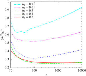
Figure 4: (Color online) $\langle\Delta x^{2}\rangle_{t}/t$ as a function of $\log t$ in the zigzag model with the same parameters as in Fig. 2.

II.2 Integrated velocity autocorrelation function

For a system with normal diffusion we define the diffusion coefficient $D$ as the asymptotic growth rate $\lim_{t\to\infty}\frac{1}{2t}\langle\Delta x^{2}\rangle_{t}$ of the mean squared displacement. The Green–Kubo formula $D=\lim_{t\to\infty}\int_{0}^{t}C(\tau)\mathrm{d}\,\tau$ Reichl (1998) relates $D$ to the velocity autocorrelation function $C(t)=\langle v_{t}\,v_{0}\rangle$: $D$ exists, and the diffusion is normal, only if $C(t)$ decays faster than $1/t$ as $t\to\infty$. $C(t)$ was studied in Alonso et al. (2004) for a different channel geometry, but this function is very noisy and it is not possible to determine its decay rate.

Instead, following Lowe and Masters (1993) we consider the integrated velocity autocorrelation function

$$R(t):=\int_{0}^{t}C(\tau)\mathrm{d}\,\tau=\langle v_{0}\,\Delta x_{t}\rangle,$$ (2)

where $\Delta x_{t}:=x(t)-x(0)$ is the particle displacement at time $t$. This function is much smoother than $C(t)$, and satisfies $R(t)\to D$ as $t\to\infty$ if the diffusion coefficient exists, whilst $R(t)\sim\ln t$ if $C(t)$ decays as $t^{-1}$.

Figure 5 plots $R(t)$ as a function of $\ln t$ for several finite and infinite horizon non-parallel zigzag models. The flatness of $R(t)$ in the finite horizon models indicates that the limit exists, and hence that the diffusion is normal, and contrasts with the asymptotic linear growth in the infinite horizon models, providing further evidence of the marginally anomalous behavior in the latter case.

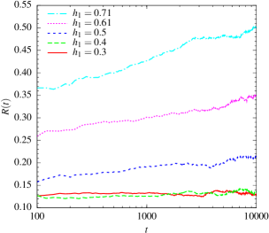
Figure 5: (Color online) Integrated velocity autocorrelation function $R(t)$ as a function of $\log t$ in the (non-parallel) zigzag model with the same parameters as in Fig. 2 ($h_{2}=0.77$ and $h_{3}=0.45$).

II.3 Higher-order moments

We define the growth exponent $\gamma_{q}$ of the $q$th moment $\langle\left|x\right|^{q}\rangle_{t}$ by

$$\gamma_{q}:=\lim_{t\to\infty}\frac{\log\langle\left|x\right|^{q}\rangle_{t}}{\log t},$$ (3)

which ignores corrections to power-law growth and is a convex function of $q$; further, $\gamma_{q}\leq q$ for all $q$, since the particles have finite velocity Armstead et al. (2003). The exponents $\gamma_{q}$, and in particular the diffusion exponent $\alpha=\gamma_{2}$, are measured using a fit to the long-time region of a double logarithmic plot of the relevant moment, assuming that the asymptotic regime has been reached.

We find that the behavior of moments of high order ($q\geq 4$) is dominated by the extreme particles, i.e. by those which have the largest value of $\left|x(t)\right|$, giving data which is not reproducible between different runs. For this reason we eliminate the $5$ most extreme particles from the average before calculating the growth rate, resulting in data which is now reproducible. A similar procedure was used in Zaslavsky and Edelman (2001).

Figure 6 shows the exponents $\gamma_{q}$ for the zigzag model with finite and infinite horizon. The low-order exponents satisfy $\gamma_{q}=q/2$, and in both cases there is a crossover to a second linear regime with slope $1$, which occurs at approximately $q=3$ in the finite horizon case and $q=2$ for infinite horizon; the latter agrees with the result found in Armstead et al. (2003) for the infinite horizon Lorentz gas using a method which also applies here. Higher-order moments thus provide another method to distinguish between normal and marginal anomalous diffusion in polygonal billiards.

The observed qualitative change in behavior of the moments corresponds to a change in relative importance between diffusive and ballistic effects Armstead et al. (2003); Castiglione et al. (1999); Ferrari et al. (2001), and explains the previous observation that the Burnett coefficient, defined as the growth rate of the fourth cumulant $\langle x^{4}\rangle_{t}-3\langle x^{2}\rangle_{t}^{2}$, diverges as a function of time in polygonal billiards Dettmann and Cohen (2001); Alonso et al. (2002).

The combination of the above tests provides strong evidence of the distinction between normal diffusion in finite horizon models and marginally anomalous diffusion in infinite horizon models.

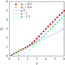
Figure 6: (Color online) Growth rate $\gamma_{q}$ of $q$th moment $\langle|x|^{q}\rangle_{t}$ for finite horizon ($h_{1}=0.4$) and infinite horizon ($h_{1}=0.5$) in the zigzag model with $h_{2}=0.77$ and $h_{3}=0.45$ for $10^{6}$ initial conditions.

III Anomalous diffusion

Whilst we generically find normal diffusion, for certain exceptional geometrical configurations this does not occur. The main exception is when there are accessible parallel scatterers in the unit cell of a model. In this case we always find anomalous (super-)diffusion, i.e. $\langle\Delta x^{2}\rangle_{t}\sim t^{\alpha}$ with $\alpha>1$: see Fig. 7. Since the particles have finite speed, we always have $\alpha\leq 2$, with the value $2$ corresponding to ballistic motion. Sub-diffusion ($\alpha<1$) was reported in Alonso et al. (2002) in a model with one rational angle, but we are not aware of any model with irrational angles exhibiting sub-diffusion.

We say that a model has ‘accessible parallel scatterers’ when there are trajectories which can propagate arbitrarily far by colliding only with scatterers which are parallel to some other scattering element in the unit cell.

As an example, the results we report for the polygonal Lorentz model were obtained with a square central obstacle, that is, a scatterer whose opposite sides are parallel. This alone does not, however, imply that the system exhibits anomalous diffusion, since it is not possible for a particle to propagate by colliding only with (copies of) this square, i.e. the scatterers making up the square are not ‘accessible’ from one another.

Any particle must in fact also collide with the top and bottom scattering walls. Only if these walls are also accessibly parallel as defined above (i.e. have parallel partners in the unit cell) do we find anomalous diffusion. Furthermore, if we alter the central obstacle shape so that it no longer has parallel sides, then we still find anomalous diffusion provided that the scattering walls still have parallel partners which are accessible from one cell to another.

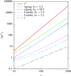
Figure 7: (Color online) Mean squared displacement $\langle\Delta x^{2}\rangle_{t}$ for parallel models versus $t$ on a double logarithmic plot. The upper and lower lines are proportional to $t$ and $t^{2}$ for comparison. The remaining curves show, from top to bottom, the parallel zigzag model with $h_{1}=0.1$ and $h_{3}=5.2,10.2$ (both shifted vertically for clarity), and the parallel polygonal Lorentz model with $h_{1}=0.1$, $w=0.15$ and $h_{3}=5.2,10.2$. Statistical errors are slightly greater than the width of the lines.

Figure 8 shows the behavior of the anomalous diffusion exponent $\alpha$ as a function of $h_{3}$ in the parallel zigzag and polygonal Lorentz models with finite horizon. The representative error bars shown give the standard deviation of the exponent over $100$ independent simulations for the same value of $h_{3}$, and indicate that the structure visible in the curve for the zigzag model is not an artifact.

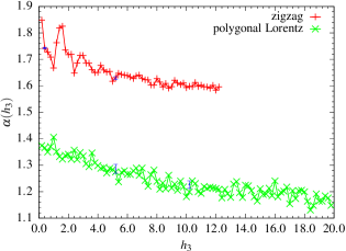
Figure 8: (Color online) Diffusion exponent $\alpha$ as a function of $h_{3}$ in the parallel zigzag model with $h_{1}=0.1$ and the parallel polygonal Lorentz model with $h_{1}=0.1$ and $w=0.15$, calculated using $10^{5}$ initial conditions evolved until the presumed asymptotic regime. (Note that at $h_{3}=1=d$ there is a rational angle in both models.) Representative error bars show the standard deviation of the exponent over $100$ independent simulations.

Figure 9 shows the growth exponent $\gamma_{q}$ as a function of $q$ in two models with anomalous diffusion. Again we find a crossover between two linear regimes, with $\gamma_{q}$ of the form Castiglione et al. (1999)

$$\gamma_{q}=\begin{cases}\nu_{1}q,&\text{for }q<q_{\text{c}}\\ q-\nu_{2},&\text{for }q>q_{\text{c}}.\end{cases}$$ (4)

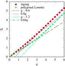
Figure 9: (Color online) Growth exponent $\gamma_{q}$ of moments for the parallel polygonal Lorentz and zigzag models with $h_{1}=0.51$, $h_{2}=h_{3}=10.0$ and $w=0.21$.

III.1 Time evolution of densities

A feature typical of normal diffusive systems is that the probability distribution of displacements (or equivalently of positions) converges in the long-time limit, when rescaled by $\sqrt{t}$, to to a normal distribution Sanders (2005). We find this behavior numerically in both of the classes of polygonal billiard channels studied here, in the cases for which the mean squared displacement grows linearly, and we conjecture that this holds in general, providing a stronger sense in which polygonal billiards can be considered diffusive.

For anomalous diffusion with $\langle\Delta x^{2}\rangle_{t}\sim t^{\alpha}$ ($\alpha>1)$, we no longer expect the central limit theorem to hold. The inset of Fig. 10 shows the probability density $\rho_{t}(x)$ of positions $x(t)$ in a parallel polygonal Lorentz model. It exhibits a striking fine structure, similar to that found in normally diffusive Lorentz gases and polygonal billiards in Sanders (2005), where it was shown that the principal contribution to this fine structure arises from a geometrical effect, namely that the amount of vertical space available for particles to occupy varies along the channel. Assuming that the dynamics has good mixing properties, it was shown that defining the demodulated density $f_{t}(x)$ by

$$f_{t}(x):=\rho_{t}(x)/h(x)$$ (5)

eliminates much of the fine structure. Here, $h(x)$ is the height of the available space in the billiard channel at horizontal coordinate $x$, normalised by the area of the unit cell so that the integral $\int_{-d}^{d}h(x)\mathrm{d}\,x$ over the unit cell is $1$. This demodulated density is also shown in the inset of Fig. 10, although the demodulation is not as effective as in the normally diffusive cases studied in Sanders (2005), due to the weaker mixing properties of the current model.

Rescaling the demodulated position density $f_{t}(x)$ at time $t$ by

$$\tilde{f}_{t}(x):=t^{\alpha/2}\,f_{t}(x\,t^{\alpha/2})$$ (6)

gives a bounded variance as $t\to\infty$ Prosen and Znidaric (2001). The main part of Figure 10 shows demodulated densities rescaled in this way for different times, compared to a Gaussian with the corresponding variance. The rescaled densities converge at long times to a non-Gaussian limiting shape, as has previously been found in other systems with anomalous diffusion Metzler and Klafter (2000).

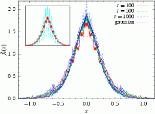
Figure 10: (Color online) Rescaled demodulated densities in the polygonal Lorentz model, compared to a Gaussian with the corresponding variance. The inset shows the original and demodulated (heavy line) densities for $t=100$. The model parameters are $h_{1}=0.1$, $h_{2}=h_{3}=0.45$, $w=0.2$, $d=1$.

III.2 Mechanism for anomalous diffusion

III.2.1 Continuous-time random walk approach

For the parallel zigzag model, Figure 13 demonstrates the presence of long laminar stretches, i.e. periods of motion during which a particle’s velocity component parallel to the channel wall does not change sign. Typical trajectories exhibit such behavior, sometimes over very long periods of time. Figure 11 shows a scatterplot representing the joint distribution $\psi(x,t)$ of laminar stretches of duration $t$ with horizontal displacement $x$ along the channel. (To compute these data, the channel was divided into sections lying between adjacent maxima and minima in order to determine the wall direction).

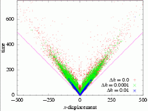
Figure 11: (Color online) Scatterplot representing the joint density $\psi(x,t)$ of laminar stretches in the zigzag model with $h_{1}=0.1$, $h_{3}=0.3$ and $h_{2}=h_{3}+\Delta h$. The straight lines with slope $1$ correspond to the maximum possible speed.

Thus, we may attempt to describe the dynamics of this system as a continuous-time random walk (CTRW), whose steps are the laminar stretches: see e.g. Weiss (1994); Zumofen and Klafter (1993). To this end, we note that Figure 11 shows that the distribution $\psi(x,t)$ is concentrated on diagonal lines emanating from the origin, which leads us to try an approximation of the form $\psi(x,t)=\textstyle\frac{1}{2}\delta(\left|x\right|-vt)\,\psi(t)$ for some speed $v$. This version of the CTRW was termed the velocity model in Zumofen and Klafter (1993), and describes motion at a constant velocity for a time $t$ in the direction $x$; after each stretch the direction is randomised and a new step is taken. With this form for $\psi(x,t)$, the long-time growth of the mean squared displacement depends on the asymptotic decay rate of the marginal distribution $\psi(t)$ of step times Zumofen and Klafter (1993): if $\psi(t)\sim t^{-1-\nu}$ as $t\to\infty$, then the variance $\sigma^{2}(t)$ behaves like $\sigma^{2}(t)\sim t^{3-\nu}$ when $1<\nu<2$, while we have normal diffusion $\sigma^{2}(t)\sim t$ for $\nu>2$.

Figure 12 shows the tail region of $\Psi(t):=1-\int_{0}^{t}\psi(\tau)\mathrm{d}\,\tau$. From the top curve we find a long-time power-law decay $\Psi(t)\sim t^{-1.58}$ for a particular case having parallel scatterers. For close-to-parallel configurations, the tail of the distribution follows that for the parallel case, but with an exponential cut-off, as shown in the inset of Fig. 12. According to the CTRW model, this cut-off gives rise to normal diffusion in the asymptotic long-time regime. This change of behavior is in qualitative agreement with our observations. Unfortunately, the value of the tail exponent for the parallel case corresponds to $\nu=1.58$ and hence to a mean squared displacement $\sigma^{2}(t)\sim t^{3-1.58}=t^{1.42}$, which does not agree with the numerically observed growth rate $\sigma^{2}(t)\sim t^{1.81}$.

Although the above results rest on a rather gross approximation to the joint distribution $\psi(x,t)$, we doubt that a more general CTRW model, incorporating information on the complete $\psi(x,t)$, would substantially improve the agreement. The reason is that correlations between consecutive laminar trajectories have an important effect not accounted for by CTRW models. Indeed, for a given trajectory, we find that the lengths of consecutive long laminar stretches are often nearly equal, indicating that the trajectory repeats very closely its previous behavior many times.

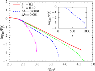
Figure 12: (Color online) Tail of $\Psi(t)$ for the parallel zigzag model. The top curve is for $h_{1}=0.1$ and $h_{3}=0.3$. The lower three curves are for $h_{1}=0.49$, $h_{3}=5.1$ and $\Delta h=0$, $0.0001$ and $0.001$ (top to bottom). The inset is a semilogarithmic plot of the $\Delta h=0.001$ case, showing exponential decay.

III.2.2 Propagating periodic orbits

On the other hand, our results indicate that it is the presence of accessible parallel scatterers that gives rise to anomalous diffusion. We believe that propagating periodic orbits, i.e. orbits which repeat themselves with a spatial displacement, may provide a mechanism for this behavior. Such orbits are more prevalent when there are parallel scatterers, since in this case it is much easier for a particle to regain its original angle of propagation after a given number of bounces, and, then, possibly repeat its previous motion. In addition, periodic orbits in polygonal billiards occur in families Galperin et al. (1995); several such families are shown in Fig. 13.

Furthermore, trajectories with initial conditions which are close in phase space to those of a propagating periodic orbit will shadow it, and hence propagate, for a long time, with a longer shadowing time for closer initial conditions. Anomalous diffusion should then result from a balance between the ballistic propagation of the periodic orbits themselves, the long-lasting ballistic motion of shadowing orbits, and the diffusive motion of other trajectories.

We have, however, not yet been able to account analytically for anomalous diffusion in this way. For instance, the mere existence of propagating orbits is not enough to give rise to the kind of anomalous behavior we observe. Indeed, families of propagating orbits exist in the corridors of the infinite-horizon periodic Lorentz gas, but these give rise only to marginally anomalous diffusion $\langle\Delta x^{2}\rangle\sim t\ln t$ Bleher (1992) (see Sec. II). Thus, although the set of propagating periodic orbits must have measure zero in phase space, since otherwise their ballistic nature would result in overall ballistic transport with $\langle\Delta x^{2}\rangle\sim t^{2}$, they must be plentiful in some sense, in order to give rise to anomalous transport. For example, such orbits could be dense at least in some parts of phase space.

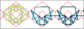
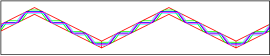
Figure 13: (Color online) Families of trapped and propagating periodic orbits in parallel systems.

IV Crossover from normal to anomalous diffusion

Since anomalous diffusion occurs only for special geometrical configurations, it is of interest to study the crossover from normal to anomalous diffusion as such configurations are approached. We begin by considering the polygonal Lorentz channel, in which we fix all geometrical parameters except for $h_{2}$, which we vary as $h_{2}=h_{3}+\Delta h$.

Figure 14 shows a double logarithmic plot of the mean squared displacement in a polygonal Lorentz model for values of $\Delta h$ tending to $0$, i.e. approaching the parallel configuration; a linear fit to the bottom curve has been subtracted from each curve for clarity. As $\Delta h$ tends to $0$, the curve for the parallel configuration ($\Delta h=0$) is followed for progressively longer times before a crossover occurs to asymptotic diffusive behaviour, which appears on the figure as a zero slope. Defining the crossover time $T_{c}(\Delta h)$ as the intersection of the initial anomalous growth with a straight line fit to the asymptotic normal growth, we find that $T_{c}$ scales like $T_{c}\sim(\Delta h)^{-0.37}$ as $\Delta h\to 0$.

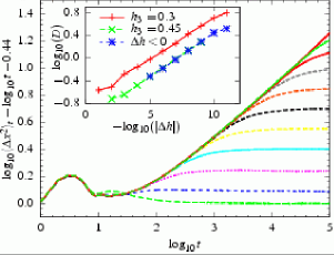
Figure 14: (Color online) Double logarithmic plot of $\langle\Delta x^{2}\rangle_{t}$ as a function of time for the polygonal Lorentz model with $h_{1}=0.1$, $h_{3}=0.45$, $w=0.2$ and $h_{2}=h_{3}+\Delta h$. Deviations from an asymptotic linear fit to the lowest curve are shown for $\Delta h=0$ (uppermost) and $\Delta h=10^{-m}$, $m=2,\ldots,11$ (bottom to top). The inset shows a double logarithmic plot of the diffusion coefficient $D$ as a function of $\Delta h$ for the polygonal Lorentz model with $h_{1}=0.1$ for $h_{3}=0.3,0.45$, and for $h_{3}=0.45$ with $\Delta h<0$.

The inset of Fig. 14 shows the diffusion coefficient $D$ as a function of $\Delta h$, obtained from the asymptotic slope of the mean squared displacement. Although Fig. 14 shows that the asymptotic linear regime has not been reached for the smallest values of $\Delta h$, thereby underestimating the diffusion coefficient, we obtain a straight line on a double logarithmic plot of $D$ versus $\Delta h$, giving the power-law behavior

$$D(\Delta h)\sim\left|\Delta h\right|^{-0.15}\quad\text{as }\left|\Delta h\right|\to 0,$$ (7)

with the same exponent for both positive and negative values of $\Delta h$ and for two (close) values of $h_{3}$. For this model, the diffusion exponent in the parallel ($\Delta h=0$) case is $\alpha\simeq 1.40$.

A similar crossover to anomalous diffusion occurs near to the parallel configuration in the zigzag model (not shown), and we conjecture that such crossover behavior is generally found in polygonal billiards near to configurations exhibiting anomalous diffusion. The rate of growth of the diffusion coefficient for $\Delta h\neq 0$ depends, however, on the diffusion exponent for $\Delta h=0$: for the zigzag model with $h_{1}=0.1$ and $h_{3}=0.3$, we find $D\sim\left|\Delta h\right|^{-0.32}$, with a diffusion exponent $\alpha\simeq 1.81$ for the parallel case; both of these exponents differ from the results in the polygonal Lorentz model.

The growth of the diffusion coefficient close to a parallel case thus depends on the anomalous diffusion exponent found in that parallel case. Indeed, the relation between the exponents characterizing the crossover from normal to anomalous transport can be obtained from the following simple scaling argument. Define the crossover time exponent $\nu$ by $T_{c}\sim|\Delta h|^{-\nu}$. We have

$$\langle x^{2}(\Delta h)\rangle_{t}\sim\begin{cases}D(\Delta h)t,&\text{for }t>T_{c}\\ t^{\alpha},&\text{for }t<T_{c},\end{cases}$$ (8)

so that continuity at $T_{c}$ gives $D(\Delta h)\sim T_{c}^{\alpha-1}\sim|\Delta h|^{\nu(1-\alpha)}$, which is in good quantitative agreement with our results.

Furthermore, this argument implies that plots of $|\Delta h|^{\nu\alpha}\langle x^{2}(\Delta h)\rangle_{t}$ as a function of $u:=|\Delta h|^{\nu}t$ should collapse onto a scaling function of the form

$$\phi(u)\sim\begin{cases}u,&\text{for }u\gg 1\\ u^{\alpha},&\text{for }u\ll 1.\end{cases}$$ (9)

The data collapse for both the zigzag and the polygonal model near a configuration of parallel scatterers is shown in Fig. 15. Interestingly, while the transport exponent $\alpha$ is sensitive to the geometrical details of the models, the best collapse was obtained for the same value of $\nu=0.37$ in both cases.

Figure 15: (Color online) Data collapse of $|\Delta h|^{\nu\alpha}\langle x^{2}(\Delta h)\rangle_{t}$ as a function of $u=|\Delta h|^{\nu}t$ for the zigzag model with $h_{1}=0.1$, $h_{3}=0.3$, which has $\alpha\simeq 1.81$ (upper curve) and the polygonal Lorentz model with $h_{1}=0.1$, $h3=0.45$, with $\alpha=1.40$. In both models the value $\nu=0.37$ was used, and curves are shown for $\Delta h=10^{-m}$, $m=4,\ldots,11$. The solid lines show the extreme behaviors of the scaling function (9).

Finally, it should be noted that the above calculations all refer to irrational angles; the situation when the value of $\Delta h$ renders an angle rational is unclear.

V Discussion and Conclusions

We have demonstrated that the type of diffusive behavior exhibited by periodic polygonal billiard channels depends on geometrical features of the unit cell. Based on our results, we conjecture that sufficient conditions for a periodic polygonal billiard channel to exhibit normal diffusion are the following: (i) all vertex angles are irrationally related to $\pi$; (ii) the billiard has a finite horizon; and (iii) there are no accessible parallel scatterers in the unit cell.

When there is an infinite horizon, diffusive transport is replaced by marginal anomalous diffusion with $\langle\Delta x^{2}\rangle\sim t\ln t$, while if there are accessible parallel scatterers, then anomalous diffusion with $\langle\Delta x^{2}\rangle\sim t^{\alpha}$, $\alpha>1$ is observed.

In the zigzag model we also have evidence of anomalous diffusion (e.g. with exponent $1.16$ for one particular model) with irrational angles chosen such that one angle is twice the other, i.e. with a rational relation between them, in disagreement with the result found in Jepps and Rondoni (2006) (where a rather small number of initial conditions was used). For other angle ratios we do not have conclusive data, but the exponents are seemingly close to $1$, while for the polygonal Lorentz model we find normal diffusion in similar situations. For the zigzag model we must thus also exclude the possibility of rationally-related angles from the above conditions for normal diffusion.

We remark that in Alonso et al. (2004), propagating periodic orbits were conjectured to be related to anomalous diffusion in a system with one rational angle, but no reason was given for their existence. Actually, it is possible to include that system into our picture by unfolding the rational angle, which gives rise to an equivalent system with parallel scatterers.

We believe that the explanation of anomalous diffusion should be found in terms of such propagating periodic orbits, which are much more prevalent in the presence of parallel scatterers. We further showed that there is a crossover from normal to anomalous diffusion as a parallel configuration is approached, with the diffusion coefficient having a power-law divergence. We hope to achieve a quantitative description of both of these points in the future.