Field-induced Berezinskii-Kosterlitz-Thouless transition and string-density plateau in the anisotropic triangular antiferromagnetic Ising model

Abstract

The field-induced Berezinskii-Kosterlitz-Thouless (BKT) transition in the ground state of the triangular antiferromagnetic Ising model is studied by the level-spectroscopy method. We analyze dimensions of operators around the BKT line, and estimate the BKT point $H_{\rm c}\simeq 0.5229\pm 0.001$, which is followed by the level-consistency check to demonstrate the accuracy of our estimate. Further we investigate the anisotropic case to clarify the stability of the field-induced string-density plateau against an incommensurate liquid state by the density-matrix renormalization-group method.

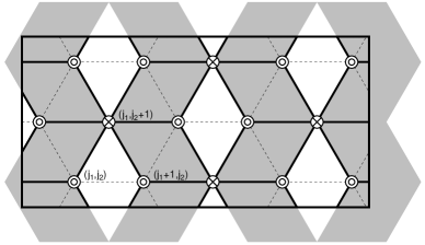
Figure 1: An example spin configuration with the $\sqrt{3}\times\!\sqrt{3}$ structure. The $j$th site is specified by two integers $(j_{1},j_{2})$ as labeled. The long (short) side of the rectangle frame is in the $x_{1}$ ($x_{2}$) direction. The spins on two (one) of three sublattices $\Lambda_{0}$ and $\Lambda_{1}$ ($\Lambda_{2}$) are parallel $\circledcirc$ (antiparallel $\otimes$) to the field direction. Four gray stripes in the $x_{2}$ direction give the string representation of the spin configuration.

It was exactly proven that the nearest-neighbor (NN) antiferromagnetic Ising model on the triangular lattice shows no phase transition at finite temperature, and possesses a ground-state ensemble carrying the finite residual entropy per spin, $S\simeq 0.3231k_{\rm B}$ Wann50 . This circumstance stems from the frustration effect that not all spins at the corners of each elementary triangle can be energetically satisfied, and then brings about the power-law decays of the correlation functions of physical quantities in the ground state Step70 . There is a long history of research on various types of perturbation effects on this ground-state degeneracy Blot91 ; Blot93 ; Kinz81 ; Qian04a ; Qian04 ; Noh_95 , where, as we will see in the following, the exact mapping to the so-called triangular Ising solid-on-solid (TISOS) model Blot82 ; Nien84 followed by a coarse graining provides an effective field theory to describe the low-energy physics Jose77 . In addition, it should be remarked that the ground-state spin configurations can be classified according to the number of strings (see below) Blot82 , which provides an intuitive connection to one-dimensional (1D) quantum systems with global U$(1)$ symmetry under the path-integral representation.

In this paper, we treat an anisotropic triangular antiferromagnetic Ising model (TAFIM) under a magnetic field; its reduced Hamiltonian ${\cal H}=\beta H_{\rm TAFIM}$ is given as

$${\cal H}(K_{1},\mu,H)=\sum_{\langle j,k\rangle}K_{jk}\delta_{\sigma_{j},\sigma_{k}}-H\sum_{j}\delta_{\sigma_{j},0}.$$ (1)

The binary variable $\sigma_{j}=0,1$ is on the $j$th site of the triangular lattice $\Lambda$ which consists of interpenetrating three sublattices $\Lambda_{l}$ $(l=0,1,2)$, and the first (second) sum runs over all NN pairs (sites). The AF coupling $K_{jk}$ takes two values $K_{1}+\mu$ or $K_{1}$ depending on whether the bond ${\langle j,k\rangle}$ lies in the $x_{1}$ direction or not (see Fig. 1). Here we define a quantity $Q=\sum_{j_{1}}N_{j_{1},j_{2}}$ with $N_{j_{1},j_{2}}=1-\delta_{\sigma_{j_{1},j_{2}},\sigma_{j_{1}+1,j_{2}}}$ for all $j_{2}$, and further restrict ourselves to the zero temperature case $K_{1}\to\infty$. Then $Q$ is independent of $j_{2}$ and the Boltzmann weight per row is given by $e^{\mu Q}$. Therefore, the anisotropy parameter $\mu$ plays a role of the chemical potential to control the number of strings (an example of the string representation is given in Fig. 1) Blot82 . Our main goal is to clarify the phase diagram of the model (1) in its ground state $K_{1}\to\infty$. For this, we shall use the level-spectroscopy (LS) method Nomu95 to treat the Berezinskii-Kosterlitz-Thouless (BKT) transition induced by $H$ in the isotropic case $\mu=0$. On the other hand, for the anisotropic case $\mu\neq 0$, the Pokrovski-Talapov (PT) transition Pokr79 between a commensurate ordered phase and an incommensurate liquid phase is expected. We directly calculate the $\mu$ dependence of the number of strings by the use of the density-matrix renormalization-group (DMRG) method Whit92 . Then, we provide a reliable phase diagram.

As we will see in the following, the string degrees of freedom in which the frustration effects are encoded play a central role for both understanding the phase diagram and relating it to the magnetization plateaus observed in the 1D frustrated quantum spin systems Okun02 . This comes from the fact that the quantity $Q$ corresponds to the uniform magnetization, and thus $\mu$ can be regarded as the magnetic field in the quantum spin systems. Further, quite recently, the string representation has been also employed in investigations of the 2D frustrated quantum magnets Jian05 , so the precise analysis on the present fundamental model may also offer a hint for a further understanding of quantum systems.

Table 1: Estimates of $H_{\rm c}$. We label the estimate by the spin-wave excitation (the vortex excitation) as KT1 (KT2). We also give the results by the phenomenological renormalization-group (PRG) and the level-spectroscopy (LS) methods.

	Reference	Method	Extrapolation		$H_{\rm c}$	Error
	Blot91	KT1	A rough estimate		0.6	—
	Blot93	KT1	Iterated fit		0.532	$\pm$0.02
	Qian04	KT2	Iterated fit		0.52	$\pm$0.04
	Quei99	PRG	Finite-size scaling		0.422	$\pm$0.014
	This work	LS	Polynomial fit		0.5229	$\pm$0.001

Now we shall start with the isotropic case $\mu=0$. For $H=0$, from the exact asymptotic behavior of the spin-spin correlation function the scaling dimension of the staggered magnetization ($S$) is given by $x_{S}=\frac{1}{4}$ Step70 , while the dimension of the uniform magnetization ($s$) is by $x_{s}=\frac{9}{4}$ Nien84 . Thus the magnetic field is irrelevant, and the critical region continues up to a certain value $H_{\rm c}$. For $H>H_{\rm c}$, the criticality of the ensemble disappears and the threefold-degenerate ground state with the $\sqrt{3}\times\!\sqrt{3}$ structure of the sublattice is realized, where a majority spin is in the field direction (see Fig. 1). The transition at $H_{\rm c}$ is the BKT type, and is described, in the scaling limit, by the 2D sine-Gordon Lagrangian density Jose77

$${\cal L}[\phi]=\frac{1}{2\pi K}\left(\nabla\phi\right)^{2}+\frac{y}{2\pi\alpha^{2}}\cos 3\sqrt{2}\phi,~{}~{}~{}K\simeq\frac{4}{9},$$ (2)

where $y\propto H$ and the continuous field in the 2D Euclidean space $(x_{1},x_{2})$ proportional to the height variable of the TISOS model satisfies $\sqrt{2}\phi+2\pi=\sqrt{2}\phi$ Comm1 . Since the lattice model is not exactly solvable, there have been several attempts to numerically estimate $H_{\rm c}$: Blöte and Nightingale investigated this problem in detail by the transfer-matrix method Blot91 ; Blot93 . Actually, they evaluated finite-size estimates $H_{\rm c}(L)$ by numerically solving the equation for the scaled gap, i.e., the so-called KT criterion $x_{S}(H,L)=\frac{2}{9}$ (this is referred to as KT1 in Table 1). Then, in order to accelerate the slow convergence of $H_{\rm c}(L)$, the iterated fits with taking account of the logarithmic correction were performed (for a more recent estimation, see Qian04 ). On the other hand, de Queiroz et al. treated the same model by the phenomenological renormalization-group (PRG) method Quei99 ; they exhibited a much smaller value inconsistent with the previous estimations (see Ref. Qian04 ). However, it is often pointed out that PRG calculations fail to estimate the BKT points Inou99 , so their result may suffer from an inadequacy of the method. Consequently, to accurately determine $H_{\rm c}$, there still remains some difficulty.

In the studies of 1D quantum systems, however, the LS method provides an efficient way to treat the BKT transitions Nomu95 . This is also true for the investigations of 2D classical spin systems Otsu05 . Let us consider the system on $\Lambda$ with $M$ ($\to\infty$) rows in the $x_{2}$ direction of $L$ (a multiple of 3) sites in the $x_{1}$ direction wrapped on the cylinder and define the transfer matrix connecting the next-nearest-neighbor rows. Since, in our discussion, the number of the strings $Q$ (or its density $\rho=Q/L$) is the most important conserved quantity in the transfer, we explicitly specify a block of the matrix as ${\bf T}_{Q}(L)$ and denote its eigenvalues as $\lambda_{p,Q}(L)$ or their logarithms as $E_{p,Q}(L)=-\frac{1}{2}\ln|\lambda_{p,Q}(L)|$ ($p$ specifies a level). In the isotropic case, the smallest one corresponding to the ground state is in the block $Q_{0}=2L/3$ Blot93 ; Blot82 ; we shall denote it and the excitation gaps from it as $E_{{\rm g},Q_{0}}(L)$ and $\Delta E_{p,Q}(L)=E_{p,Q}(L)-E_{{\rm g},Q_{0}}(L)$, respectively. Then the conformal invariance provides direct expressions for the central charge $c$ and a scaling dimension $x_{p,Q}$ in the critical system as $E_{{\rm g},Q_{0}}(L)\simeq Lf-\pi c/6L\zeta$ and $\Delta E_{p,Q}(L)\simeq 2\pi x_{p,Q}/L\zeta$. Here $\zeta$ $(=2/\sqrt{3})$ and $f$ are the geometric factor for $\Lambda$ and a free energy per site, respectively Card84 ; Blot86 .

Blöte and Nightingale precisely checked various scaling dimensions based on the Coulomb-gas scenario Blot93 , whereas Nomura pointed out the importance of logarithmic corrections in the renormalized scaling dimensions $x(l)=\Delta E(L)/(2\pi/L\zeta)$ to determine the BKT point $(l=\ln L)$ Nomu95 . In the present effective theory (2), there are two marginal operators on the BKT point, i.e., ${\cal M}=(1/K)\left(\nabla\phi\right)^{2}$ and $s=\sqrt{2}\cos 3\sqrt{2}\phi$ which hybridize along the RG flow and result in two orthogonalized ones, i.e., the “${\mathcal{M}}$-like” and the “cos-like” operators Nomu95 . Writing the former and the latter as $O_{0}\propto\left({\cal M}+s/\sqrt{2}\right)$ and $O_{1}\propto\left(-{\cal M}/\sqrt{2}+s\right)$, their renormalized scaling dimensions can be calculated near the multicritical point; the results up to the first-order perturbations are given as follows: $x_{0}(l)\simeq 2-y_{0}\left(1+\frac{4}{3}t\right)$ and $x_{1}(l)\simeq 2+y_{0}\left(2+\frac{4}{3}t\right)$, where $(y_{0},y_{1})=(9K/2-2,y)$ and the small deviation from the BKT point $t=y_{1}/y_{0}-1$ Nomu95 . Another important operator is a relevant one, i.e., the staggered magnetization $S=\exp(\pm i\sqrt{2}\phi)$ whose dimension is expressed as $x_{S}(l)\simeq\frac{2}{9}\left(1+\frac{1}{2}y_{0}\right)$ in the same region. Consequently, the level-crossing condition,

$$x_{0}(l)=4-9x_{S}(l),$$ (3)

provides a finite-size estimate of the BKT point. Since these operators are described by $\phi$, we can calculate the renormalized scaling dimensions from excitation gaps found in the $Q_{0}$ block. Further, the symmetry properties such as the translation of one lattice spacing (or a cyclic permutation among sublattices $\Lambda_{i}$) ${\cal T}$, the space inversion ${\cal P}$, and the spin reversal ${\cal S}$ at $H=0$ are also important for the precise specification of relevant excitations levels. These symmetry operations can be interpreted in the field language as ${\mathcal{T}}$: $\sqrt{2}\phi\mapsto\sqrt{2}\phi+2\pi/3$, ${\mathcal{P}}$: $\sqrt{2}\phi\mapsto-\sqrt{2}\phi$, and ${\mathcal{S}}$: $\sqrt{2}\phi\mapsto\sqrt{2}\phi+\pi$ Blot93 ; Nien84 ; Land83 . For instance, $s$ is invariant for ${\mathcal{T}}$ and ${\mathcal{P}}$, but is odd for ${\mathcal{S}}$ as expected, while $S$ is in the $|k|=2\pi/3$ block and is odd for ${\mathcal{S}}$. Therefore, the corresponding excitations to $O_{0}$ and $O_{1}$ can be found in the subspace of the wavevector $k=0$ and the even parity for the space inversion. We calculate the excitation levels by utilizing these symmetry operations.

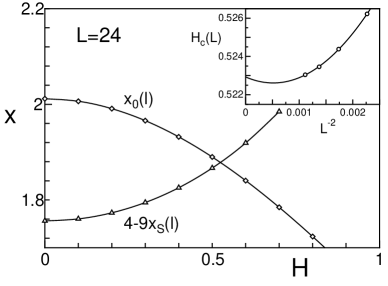
Figure 2: The spectroscopy of levels observed in the $L=24$ sites system. The crossing of $x_{0}(l)$ (diamonds) and $4-9x_{S}(l)$ (triangles) gives the finite-size estimate of the transition point $H_{\rm c}(L)$. Inset shows the extrapolation of finite-size estimates to the thermodynamic limit $L\to\infty$.

Table 2: The $L$ dependences of dimensions $x_{0}(l)$ and $x_{1}(l)$ at $H_{\rm c}$. The average $x_{\rm av}(l)$ (see text) is extrapolated to $L\to\infty$ using the least-squares fitting of the polynomial in $1/L^{2}$.

$L$	18	21	24	27	30	$\infty$
$x_{0}(l)$	1.88528	1.88110	1.87913	1.87835	1.87823	—
$x_{1}(l)$	2.40464	2.37543	2.35551	2.34096	2.32981	—
$x_{\rm av}(l)$	2.05840	2.04587	2.03792	2.03256	2.02875	2.01292

We perform the exact-diagonalization (ED) calculations of ${\bf T}_{Q_{0}}(L)$ for systems up to $L=30$. We show the level-crossing data in Fig. 2 and the extrapolation of the finite-size estimates $H_{\rm c}(L)$ to the thermodynamic limit $L\to\infty$ using the least-squares fitting of the polynomial in $1/L^{2}$ (the inset) Blot93 ; Card86 . Then we find that while our result is consistent with previous estimations, it is much more accurate owing to the fast convergence of finite-size estimates (see Table 1). Next we shall check a universal relation among excitation levels. For instance, the following relation is to be satisfied at the BKT point: $[2x_{0}(l)+x_{1}(l)]/3\simeq 2$ Nomu95 . In Table 2, we give the scaling dimensions at $H_{\rm c}$, where the left-hand side of the relation is denoted as $x_{\rm av}(l)$. Although $x_{0}(l)$ and $x_{1}(l)$ considerably deviate from the value for the free-boson case 2 due to the logarithmic corrections, their main parts cancel each other, so the average takes a value close to 2. These data provide the check of the accuracy of our estimate and the evidences to ensure that numerically studied levels have the above-mentioned theoretical interpretations.

In the rest part, we shall discuss the anisotropic case $\mu\neq 0$. As we have seen in the above, the magnetic field $H$ favors the long-range ordered commensurate (C) phase through the potential $\cos 3\sqrt{2}\phi$. On the other hand, $\mu$ which newly introduces a local density term $\partial_{1}\phi$ to the effective theory (2) tends to stabilize an incommensurate (IC) liquid phase Pokr79 ; Schu80 . Therefore, as can be found in the literature, the PT-type C-IC transition may occur Noh_95 ; Blot82 ; Noh_94 . For $H=0$, we know the exact $\mu$-$\rho$ curve $\rho(\mu)=\arccos\left(1/2e^{2\mu}-1\right)/\pi$ which is given in Fig. 3 Blot82 . On the other hand, for $H\neq 0$, we employ numerical methods and estimate the curve from the finite-size system data as $\mu\simeq\left[E_{{\rm g},Q+2}(L)-E_{{\rm g},Q}(L)\right]/2$ Noh_95 . While, like the exact solid curve, $\rho$ is a smooth function of $\mu$ showing the compressive liquid state for $H\leq H_{\rm c}$, there is the string-density plateau $[\mu_{-}(H),\mu_{+}(H)]$ with $\rho=\frac{2}{3}$ for $H>H_{\rm c}$ (see the DMRG data denoted by marks). In this plot, the top and the bottom of each step correspond to $(Q+2)/L$ and $Q/L$ respectively, so we can estimate the C-IC phase boundary lines from the edges of the plateau.

In Fig. 4, we provide our phase diagram. Here it is noted that the threshold $\mu_{0}(H)$ below which the doubly degenerate vacuum of strings with $\rho=0$ is realized (see Fig. 3) is exactly given by $\mu_{0}(H)=-\ln[2\cosh(H/4)]$ Blot82 ; Lin_79 . So, we also draw it in the figure. The cross on the isotropic line $\mu=0$ shows the BKT point obtained by the LS method. For large $H$, we can use the ED data $\mu_{\pm}(H,L)=\pm\left[E_{{\rm g},Q_{0}\pm 2}(L)-E_{{\rm g},Q_{0}}(L)\right]/2$ and the extrapolation formula $\mu_{\pm}(H,L)\simeq\mu_{\pm}(H)+{\rm const}/L^{2}$ (see open circles) Saka91 . For $H\lesssim 4$, assuming the square-root behavior around the plateau, we estimate $\mu_{\pm}(H)$ from the $\rho$-$\mu$ curve obtained by DMRG. From this plot, we find that two PT-transition lines $\mu_{\pm}(H)$ seem to be terminated at the BKT point $(\mu,H)=(0,H_{\rm c})$ and that the plateau region becomes wider with the increase of the magnetic field. For $H\simeq H_{\rm c}$, it is still difficult to determine the narrow plateau region corresponding to the exponentially small energy gap even by the use of the DMRG method. However, by combining the LS result and the DMRG data, we can obtain the reliable phase diagram of our model.

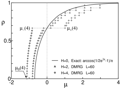
Figure 3: The $\mu$-$\rho$ curves: Triangles (diamonds) with dotted line show the DMRG data at $H=2$ ($H=4$), and the solid line exhibits the exact result at $H=0$. The flat region with $\rho=\frac{2}{3}$ corresponds to the string-density plateau $[\mu_{-}(H),\mu_{+}(H)]$. $\mu_{0}(H)$ is the threshold below which the string is absent.

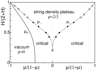
Figure 4: The ground-state phase diagram. The vacuum of strings is stabilized on the left of the solid curve $\mu_{0}(H)$. The field-induced ordered phase corresponds to the string-density plateau state with $\rho=\frac{2}{3}$. The cross on the $\mu=0$ line shows the BKT point obtained by the LS method. The filled (open) circles show estimates $\mu_{\pm}(H)$ by the DMRG (ED) method. Dotted curves give a guide to the eyes.

Lastly, we shall discuss some related topics. The magnetization process observed in the ground state of the $S=\frac{1}{2}$ anisotropic AF chain with a strong frustration exhibits the plateau at $\frac{1}{3}$ of the saturation magnetization Okun02 . This plateau state exhibits spontaneous breaking of the translational symmetry down to the period $n=3$, so it is threefold degenerate (i.e., $\uparrow\uparrow\downarrow\uparrow\uparrow\downarrow\!\cdots$), and thus satisfies the necessary condition for the magnetization plateau Oshi97 , i.e., $n(S-m)={\rm integer}$ with the average magnetization per site $m=\frac{1}{6}$. According to the bosonization treatment Lech04 , this magnetization-plateau-formation transition is described by the sine-Gordon field theory, which is identical to the present case. And more generally, since $Q$ is the conserved quantity in our system, the above necessary condition can be translated to the density plateau condition for the string systems as $n\rho={\rm integer}$, where $\rho$ is the possible density at the plateau and $n$ is the periodicity of the plateau state. For its derivation, ${\cal U}=\exp[-i\sum_{j_{1}=1}^{L}\left(2\pi j_{1}/L\right)N_{j_{1},j_{2}}]$ plays a role of the twist operator. While the present system only possesses the $\rho=\frac{2}{3}$ plateau state with the spontaneous symmetry breaking of ${\cal T}$ down to the period $n=3$, Noh and Kim intensively investigated the interacting string/domain-wall systems based on TAFIM with spatially anisotropic further-neighbor couplings Noh_94 . They used the Bethe-ansatz method to diagonalize the transfer matrix, and found the $\rho=\frac{1}{2}$ plateau phase. Furthermore the period $n=2$ of the plateau state has been suggested in that case. Therefore, we think that the above necessary condition for the plateau can provide a important viewpoint for the understandings of the interacting strings embedded in TAFIM with various extensions.

One of the authors (H.O.) thanks M. Nakamura and K. Nomura for stimulating discussions. This work was supported by Grants-in-Aid from the Japan Society for the Promotion of Science.

References

- (1) G.H. Wannier, Phys. Rev. 79, 357 (1950); Phys. Rev. B 7, 5017 (1973); R.M.F. Houtappel, Physica (Amsterdam) 16, 425 (1950).
- (2) J. Stephenson, J. Math. Phys. 11, 413 (1970).
- (3) H.W.J. Blöte, M.P. Nightingale, X.N. Wu, and A. Hoogland, Phys. Rev. B 43, 8751 (1991).
- (4) H.W.J. Blöte and M.P. Nightingale, Phys. Rev. B 47, 15046 (1993).
- (5) W. Kinzel and M. Schick, Phys. Rev. B 23, 3435 (1981); J.D. Noh and D. Kim, Int. J. Mod. Phys. B 6, 2913 (1992).
- (6) J.D. Noh and D. Kim, Phys. Rev. E 51, 226 (1995).
- (7) X. Qian and H.W.J. Blöte, Phys. Rev. E 70, 036112 (2004).
- (8) X. Qian, M. Wegewijs, and H.W.J. Blöte, Phys. Rev. E 69, 036127 (2004).
- (9) H.W.J. Blöte and H.J. Hilhorst, J. Phys. A 15, L631 (1982).
- (10) B. Nienhuis, H.J. Hilhorst, and H.W.J. Blöte, J. Phys. A 17, 3559 (1984).
- (11) J.V. José, L.P. Kadanoff, S. Kirkpatrick, and D.R. Nelson, Phys. Rev. B 16, 1217 (1977).
- (12) K. Nomura, J. Phys. A 28, 5451 (1995).
- (13) V.L. Pokrovsky and A.L. Talapov, Phys. Rev. Lett. 42, 65 (1979).
- (14) S.R. White, Phys. Rev. Lett. 69, 2863 (1992); Phys. Rev. B 48, 10345 (1993).
- (15) K. Okunishi and T. Tonegawa, J. Phys. Soc. Jpn. 72, 479 (2003); Phys. Rev. B 68, 224422 (2003).
- (16) For example, see Y. Jiang and T. Emig, Phys. Rev. Lett. 94, 110604 (2005), and references therein.
- (17) The nonlinear potential is highly irrelevant, so it was dropped in our argument.
- (18) S.L.A. de Queiroz, T. Paiva, J.S. de Sá Martins, and R.R. dos Santos, Phys. Rev. E 59, 2772 (1999).
- (19) J.C. Bonner and G. Müller, Phys. Rev. B 29, 5216 (1984); J. Sólyom and T.A.L. Ziman, ibid. 30, 3980 (1984); H. Inoue and K. Nomura, Phys. Lett. A 262, 96 (1999).
- (20) H. Otsuka, K. Mori, Y. Okabe, and K. Nomura, Phys. Rev. E 72, 046103 (2005); H. Matsuo and K. Nomura, J. Phys. A 39, 2953 (2006).
- (21) J.L. Cardy, J. Phys. A 17, L385 (1984).
- (22) H.W.J. Blöte, J.L. Cardy, and M.P. Nightingale, Phys. Rev. Lett. 56, 742 (1986); I. Affleck, ibid. 56, 746 (1986).
- (23) D.P. Landau, Phys. Rev. B 27, 5604 (1983).
- (24) J.L. Cardy, Nucl. Phys. B 270 [FS16], 186 (1986).
- (25) H.J. Schulz, Phys. Rev. B 22, 5274 (1980).
- (26) J.D. Noh and D. Kim, Phys. Rev. E 49, 1943 (1994).
- (27) K.Y. Lin and F.Y. Wu, Z. Phys. B 33, 181 (1979).
- (28) For example, T. Sakai and M. Takahashi, Phys. Rev. B 43, 13383 (1991).
- (29) M. Oshikawa, M. Yamanaka, and I. Affleck, Phys. Rev. Lett. 78, 1984 (1997).
- (30) P. Lecheminant and E. Orignac, Phys. Rev. B 69, 174409 (2004).