Sum Rule Anomaly from Suppression of Inelastic Scattering in the Superconducting State

Abstract

In the conventional BCS description of a superconductor the kinetic energy increases in the superconducting state. We describe the observed decrease in kinetic energy by adopting a simple model of electrons whose elastic scattering rate undergoes a sharp decrease as the temperature is lowered below $T_{c}$. This phenomenology has been suggested by other experiments, particularly microwave conductivity. We find that such a decrease accounts for the observed increase; a study of these different phenomena over a wide range of high $T_{c}$ materials would confirm this correlation.

I introduction

Much of the focus in the high temperature cuprates has been on the normal state. In fact, although we continue to probe the superconducting state with finer probes and better samples, the general conclusion seems to be that the state is BCS-like with well-defined quasiparticles. Indications of this statement are from photoemission kaminski00 and thermal conductivity chiao00 studies on Bi2212 and YBCO, respectively. These and many other studies are converging on the general notion that, while the superconducting state has many conventional properties (albeit with an order parameter with d-wave symmetry), the normal state is in many ways anomalous.

However, optical studies over the last half dozen years have found an anomalous behaviour in the optical sum rule kubo57 , that appears in the superconducting state basov99 ; molegraaf02 ; santander-syro03 . This sum rule relates the weight of the entire oscillator strength to the bare plasma frequency; a related sum rule pertains to a single band; then optical processes involving transitions of excitations that belong only to this band must be well-separated (even in principle) from those that involve other bands. Alternatively, apparent violations may occur because higher energy processes are “left off the accounting sheet”, so to speak.

The observations, whose interpretation remains under debate, boris04 ; kuzmenko05 ; santander-syro05 can be summarized as follows. First, recall the ”single band” sum rule maldague77 ; hirsch00 ; norman02

$$\int_{0}^{+\infty}d\nu\mathop{\rm Re}\left[\sigma_{\rm xx}(\nu)\right]={\pi e^{2}\over 4\hbar^{2}}\biggl{\{}\frac{4}{N}\sum_{k}{\partial^{2}\epsilon_{k}\over\partial k_{x}^{2}}n_{k}.\biggr{\}}$$ (1)

where $\epsilon_{k}$ is the tight-binding dispersion and $n_{k}$ is the single spin momentum distribution function. We define the quantity in braces as $-<T_{\rm xx}>$. Note that in general the kinetic energy is given by $<K>=\frac{2}{N}\sum_{k}\epsilon_{k}n_{k}$, and only in the case of nearest neighbour hopping in two dimensions is $<T_{\rm xx}>=<K>$. Nonetheless we will use this case to build intuition concerning the behaviour of the sum rule. As explored in Ref. vandermarel03, , this characterization is reasonably accurate even when beyond nearest neighbour hopping is included.

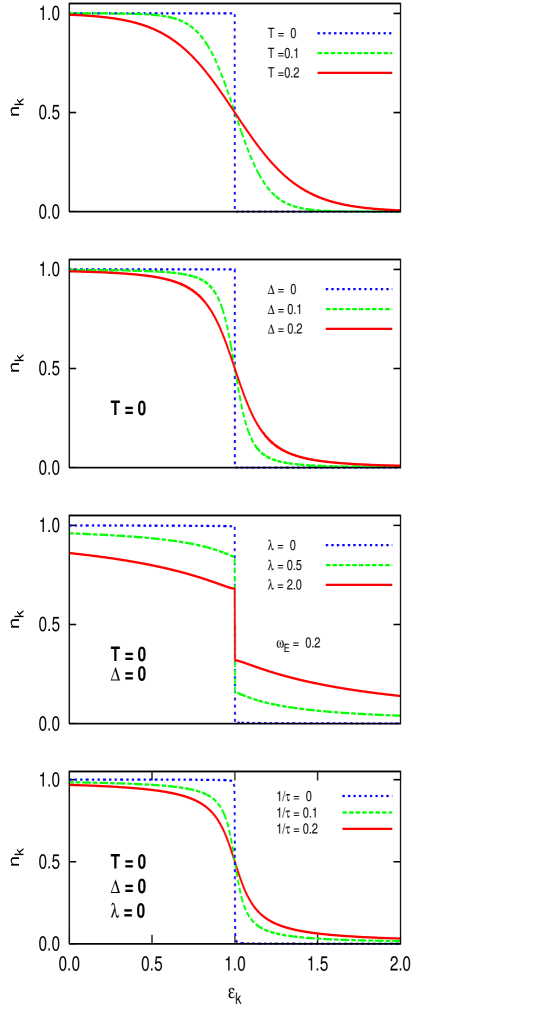
Figure 1: A summary of various reasons for why the momentum distribution is broadened. In (a) temperature is responsible for the broadening, while in (b) the occurrence of superconductivity results in broadening, even at $T=0$. In (c) and (d) inelastic scattering (as modelled by coupling to an Einstein phonon within the Migdal approximation) and elastic scattering (as modelled by impurity scattering in the Born limit) lead to the broadened distributions as shown.

The simplest situation in which one can understand Eq. 1 is the case of non-interacting electrons; then, the momentum distribution is simply given by the Fermi-Dirac function. At zero temperature this is a step function at the Fermi energy, and all the states with the lowest energy are occupied, while those with higher kinetic energy are empty. This, of course minimizes the total kinetic energy, and therefore maximizes the sum rule. As we raise the temperature, states with higher kinetic energy become partially occupied, while those with lower kinetic energy become partially empty. This behaviour is illustrated in Fig. (1a). Therefore the RHS of Eq. 1 decreases as temperature increases. The sum rule (as determined by the RHS of Eq.1) is plotted in Fig. 2 (uppermost red, solid curve) as a function of $T^{2}$. The result is mostly linear in $T^{2}$, as one can discern from the Sommerfeld expansion benfatto05 . However, note that this will depend in general on the details of the band structure, filling, etc.; careful inspection of Fig. (2) shows deviations from $T^{2}$ behaviour. This is partly caused here by the two dimensional van Hove singularity. However, other band fillings, as we have verified, also cause significant deviation from $T^{2}$ behaviour benfatto05 .

What happens when the system goes superconducting? The momentum distribution function is shown in Fig. (1b), for a gap of varying size in the quasiparticle spectrum. Keep in mind that for an order parameter with d-wave symmetry, the momentum distribution is no longer a function of the band structure energy, $\epsilon_{k}$ alone. For example, for a BCS order parameter with simple nearest neighbour form, $\Delta_{k}={\Delta\over 2}(\cos{k_{x}}-\cos{k_{y}})$, as $k$ varies from the $(0,0)$ to $(\pi,0)$, the magnitude of the order parameter changes from zero to $\Delta$, On the other hand, as $k$ varies along the diagonal (from the bottom of the band to the top), the order parameter is zero (and constant). In any event, Fig. (1b) conveys the well-known fact that even at zero temperature, BCS-like superconductivity raises the kinetic energy of the electrons. The consequence of this for the electron kinetic energy is shown in Fig. (2), for both an s-wave (green, dashed curve), and a d-wave (blue, dotted curve) order parameter. As our discussion indicated, the steady increase as the temperature is lowered is arrested at $T_{c}$, and the magnitude of the kinetic energy in general decreases below $T_{c}$. As expected, the effect is stronger for s-wave than for d-wave symmetry.

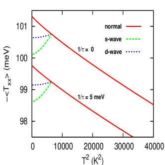
Figure 2: The optical sum rule (RHS of Eq. (1)) as a function of temperature for the clean limit (upper curves) and with elastic scattering (lower curves). Note that elastic scattering mainly just shifts the curves. An s-wave order parameter (green, dashed curve) leads to a more significant decrease in the sum rule than a d-wave order parameter (blue, dotted curve). We used a tight-binding model with nearest neighbour hopping only, as described in the text.

Briefly, then, the experimental situation molegraaf02 ; santander-syro03 is that, particularly for underdoped and optimally doped samples, the conductivity sum rule (i.e. the left-hand side (LHS) of Eq. 1) indicates an increase in the magnitude of the kinetic energy (RHS) in the superconducting state. For the purposes of this work, we assume this is the ”experimental fact” and defer doubts and debates to Refs. boris04, ; kuzmenko05, ; santander-syro05, (a more recent work is Ref. carbone05, ).

Interestingly, this very scenario was predicted hirsch92 well before experiments with the required accuracy were performed. The basis for this prediction was that the electron (or hole) kinetic energy can, in principle, change upon entering the superconducting state, so that the “single band” sum rule, Eq. 1 would not remain constant. In particular spectral area from relatively very high energy would change at the superconducting transition. Since this spectral weight is not accounted for in the single band sum rule of Eq. 1, then there would be an apparent violation. This was demonstrated to occur for the hole mechanism hirsch89 ; hirsch89a of superconductivity. In that model the effective mass of the holes decreases in the superconducting state; by pairing the holes are ’liberated’ compared to their mobility in the normal state. Partly this physics manifests itself in an effective pairing interaction which has the peculiar form obtained in Ref. hirsch89a, . In this sense these experimental results represent a ”smoking gun” that point towards the hole mechanism of superconductivity. Many details are worked out in Ref. hirsch00, .

However, other explanations have been put forth after the experiments were performed. Many have focused on the impact of superconductivity on the bosonic spectral function, i.e. on the boson that is thought to mediate the pairing. For example, in Ref. norman02, a frequency-dependent scattering rate was assumed, that underwent a significant reduction in the superconducting state. A similar modelling was implemented in Ref. knigavko04, and Ref. schachinger05, . In each case, a change was put in by hand; in the first case they were largely motivated by the Angular Resolved PhotoEmission Spectroscopy (ARPES) results kaminski01 , while in the latter two the appearance of a sharp neutron resonance mode rossat-mignod91 provided the motivation for an abrupt change. In fact, in Ref. schachinger05, this latter scenario was explored in more detail with models used for the spin fluctuations that have described a number of other experiments.

The purpose of this paper is to see to what extent changes to a frequency-independent scattering rate can reproduce the observed sum-rule variation. The motivation is two-fold. First, it is always helpful to simplify the description of the phenomenon as much as possible, so that presumably only the essence remains. Secondly, this follows the microwave analysis of Ref. hosseini99, , and so would bring together observations from different experiments. In that work (see also Ref. bonn92, ) a two-fluid interpretation of their results led them to a frequency-independent scattering rate whose value collapses in the superconducting state, following a $T^{4}$ power law at low temperatures. This properly accounted for the broad low temperature peak in the real part of the microwave conductivity. Indeed, the original microwave experiments nuss91 interpreted the presence of this peak in the same way; both regarded the origin of this lifetime decrease as being due to a ”gapping” of some collective mode responsible for the normal state scattering, but no longer functional in the superconducting state. This is somewhat consistent with the scenario adopted by Norman and Pépin norman02 and Knigavko et al. knigavko04 . Here, we wish to simplify the phenomenology that relates all of these experimental findings: a simple number characterizes the single electron scattering in the normal state (here this really is a “characterization”, as the normal state is very likely not even a Fermi Liquid). Thus linewidths are in general broad, as seen by ARPES, for example, and collective modes of these electrons will also be broad. A sharpening of the electron spectral function in the superconducting state leads to quasiparticle-like peaks in the ARPES, a collective mode that also sharpens, the prominent peak in the microwave conductivity, and an apparent sum-rule anomaly below $T_{c}$. We will focus on a description of the latter phenomenon. We start with a discussion of the momentum distribution function in the next section, where, in many cases an analytical form can be obtained. We then explore the impact this has on the right-hand side of the sum rule equation, Eq. (1), as a function of temperature, order parameter symmetry, band structure, and elastic scattering rate. Using the phenomenological temperature dependence of the elastic scattering rate derived from the microwave measurements we then illustrate the “anomalous sum rule behaviour”, as seen in experiment. We close with a summary and implications for experiments.

II momentum distribution functions

Returning to Fig. 1, we outline our calculations and explain the other parts. In general, the momentum distribution function is given by

$$n_{k}={1\over\beta}\sum_{m=-\infty}^{+\infty}G(k,i\omega_{m})e^{i\omega_{m}0^{+}}={1\over 2}+{1\over\beta}\sum_{m=-\infty}^{+\infty}{\rm Re}\ G(k,i\omega_{m}),$$ (2)

where $G(k,i\omega_{m})$ is the (in principle) exact single electron Green function with momentum $k$ and frequency $i\omega_{m}$. The $i\omega_{m}$ are the Fermionic Matsubara frequencies,$i\omega_{m}=\pi T(2m-1)$, where $m$ is an integer and $T$ is the temperature ($k_{B}\equiv 1$). The inverse temperature, $\beta\equiv 1/T$. The Green function $G$ is generally given by the Dyson equation,

$$G(k,z)=1/\bigl{[}z-\epsilon_{k}-\Sigma(k,z)\bigr{]},$$ (3)

where $z$ is anywhere in the complex plane, $\epsilon_{k}$ is the non-interacting dispersion, and $\Sigma(k,z)$ is the electron self energy. For the superconducting state, this equation holds when $G$ is understood to be the $G_{11}$ element of the $2\times 2$ Nambu matrix schrieffer64 .

For the RHS of Eq. 1, the calculation of the self energy for a given model and approximation suffices, and these equations are all that is required. For the LHS, the two-particle response is required, and is much more difficult. Although we have computed the LHS for various models in the past, this calculation is on less sure footing, so we will show calculations of the RHS only. First, for the non-interacting electron gas, $G_{0}(k,z)=1/\bigl{[}z-\epsilon_{k}\bigr{]}$, and the result from Eq. 2 is the Fermi function. This is what is plotted in Fig. 1a for the various temperatures indicated, all in units where the bandwidth is 2, and the chemical potential (hidden in $\epsilon_{k}$) is in the middle of the band.

In Fig. (1b) we require the superconducting state. In this case the relevant Nambu matrix element is

$$G_{11}(k,i\omega_{m})={i\omega_{m}Z(k,i\omega_{m})+\epsilon_{k}\over(i\omega_{m})^{2}Z^{2}(k,i\omega_{m})-\phi^{2}(k,i\omega_{m})-\epsilon_{k}^{2}},$$ (4)

where the self energy is given by $\Sigma(k,i\omega_{m})\equiv i\omega_{m}\bigl{[}1-Z(k,i\omega_{m})\bigr{]}$, and an off-diagonal self energy, $\phi^{2}(k,i\omega_{m})\equiv Z(k,i\omega_{m})\Delta(k,i\omega_{m})$, is also required. In BCS-like theories it is the $\Delta(k,i\omega_{m})$ that reduces to the familiar gap parameter, $\Delta$. For the purposes of Fig. (1b) we have assumed that something has given rise to superconductivity, with a BCS order parameter, $\Delta_{k}$, whose values (constant in $k$ for this figure) are indicated. Then $Z(k,i\omega_{m})=1$ and $\Delta(k,i\omega_{m})\rightarrow\Delta_{k}$. Using Eq. 4, Eq. 2 yields the familiar schrieffer64

$$n_{k,s}={1\over 2}\biggl{(}1-{\epsilon_{k}\over E_{k}}\biggr{)},$$ (5)

where $E_{k}\equiv\sqrt{\epsilon_{k}^{2}+\Delta^{2}_{k}}$. A finite and constant order parameter clearly gives rise to smearing at what was the Fermi surface. Note that this is in the clean limit, and at zero temperature. Nonetheless, the BCS ground state is usually considered a Fermi Liquid, in the sense that well-defined quasiparticles (with energy $E_{k}$) exist, even though there is no longer a discontinuity at the chemical potential. It is clear that the onset of superconductivity causes occupation of higher kinetic energy states, just like raising the temperature does. If the onset of superconductivity more than compensates the lowering of temperature, than the trend which the kinetic energy was following with temperature will reverse itself. Fig. 2 clearly indicates that this is the case, though less so for an order parameter with d-wave symmetry than one with s-wave symmetry.

In what other ways can higher kinetic energy states be occupied? Refs. norman02, ; knigavko04, used a coupling to a phonon-like boson. Both applied the so-called Migdal approximation. Using a single mode at Einstein frequency $\omega_{E}$, coupled to the electrons with coupling constant $\lambda$, the self energy is given by

$$\Sigma_{\rm in}(i\omega_{m})=-i\lambda\omega_{E}\tan^{-1}\biggl{(}{\omega_{m}\over\omega_{E}}\biggr{)}.$$ (6)

Then the momentum distribution function for inelastic scattering becomes

$$n_{k,in}={1\over 2}-{1\over\beta}\sum_{m}{\epsilon_{k}\over\epsilon_{k}^{2}+\bigl{(}\omega_{m}+\lambda\omega_{E}{\rm tan}^{-1}\bigl{(}{\omega_{m}\over\omega_{E}}\bigr{)}\bigr{)}}.$$ (7)

In the zero temperature limit, $\omega_{m}\rightarrow\omega$, a continuous variable and the Matsubara sum becomes a continuous integral. Then it is easy to see that a discontinuity remains at the Fermi level, whose size is $1/(1+\lambda)$. Calculations are shown in Fig. (1c). Clearly increasing the coupling tends to push electrons into higher kinetic energy states. If a lowering of the electron-boson coupling were to accompany the onset of superconductivity as the temperature is lowered, the savings in kinetic energy could more than offset the squandering of kinetic energy seen in Fig. 1b due to the superconductivity itself. This has been amply discussed in Refs. norman02, ; knigavko04, , and will not be further addressed here.

The focus of this work is elastic scattering, for which we will adopt the simple Born approximation. This will make everything we compute look formally like impurity scattering (in the Born limit). However, as Hosseini et al. hosseini99 pointed out, the amount of impurities in their samples is small, and this issue has been tested under controlled impurity addition, so we are really modelling some inelastic process which, as discussed in the introduction, seems to disappear when the material goes superconducting. Elastic scattering is like static inelastic scattering, i.e. in Eq. (6) $\omega_{E}\rightarrow 0$ while $\lambda\omega_{E}\rightarrow 1/(\pi\tau)$, with $1/\tau\equiv\Gamma$ some characteristic scattering rate. Then $\Sigma_{\rm el}(k,i\omega_{m})=-i{\Gamma\over 2}{\rm sgn}(\omega_{m})$, as expected for the Born approximation. Substitution into Eq. 2 then yields, for elastic scattering,

$$n_{k,el}={1\over 2}-{1\over\pi}{\rm Im}\ \psi\biggl{(}{1\over 2}+{\bar{\Gamma}\over 2}+i\bar{\epsilon}_{k}\biggr{)},$$ (8)

where $\psi(z)$ is the diagamma function, and $\bar{q}\equiv q/(2\pi T)$. For $T=0$ one recovers the simple result

$$n_{k,el}={1\over\pi}\cot^{-1}\bigl{(}{2\epsilon\over\Gamma}\bigr{)}\phantom{aaaaa}{\rm(T=0)}.$$ (9)

This quantity is plotted in Fig. (1d). Note that at finite temperature (shown below) more impurity scattering reinforces what a higher temperature already does, i.e. it increases the kinetic energy. Thus, it should be clear that a collapse of the scattering rate will decrease the kinetic energy, and offset the trend evident in Fig. (1b).

Finally, we wish to examine the distribution function in the superconducting state. The quantities

$$Z(k,i\omega_{m}) = 1+{1\over 2\tau}{1\over\sqrt{\omega_{m}^{2}+\Delta_{k}^{2}}}$$

$$\phi(k,i\omega_{m}) = \Delta_{k}+{1\over 2\tau}{\Delta_{k}\over\sqrt{\omega_{m}^{2}+\Delta_{k}^{2}}}$$ (10)

are entered into Eq. (4), which is then inserted into Eq. (2). The result is

$$n_{k,els}=n_{0k,els}+\delta n_{k,els},$$ (11)

where

$$n_{0k,els}={1\over 2}-{\epsilon_{k}\over E_{k}}{2\over\pi}{\rm Im}\ \psi\biggl{(}{1\over 2}+{\bar{\Gamma}\over 2}+i\bar{E}_{k}\biggr{)},$$ (12)

just like Eq. (8) except that $E_{k}$ replaces $\epsilon_{k}$ at relevant places, and the additional piece,

$$\delta n_{k,els}=-{2\over\beta}\sum_{m=1}^{\infty}\biggl{[}{\epsilon_{k}\over\epsilon_{k}^{2}+\bigl{(}\sqrt{\omega_{m}^{2}+\Delta_{k}^{2}}+1/(2\tau)\bigr{)}^{2}}-{\epsilon_{k}\over\epsilon_{k}^{2}+(\omega_{m}+1/(2\tau))^{2}+\Delta_{k}^{2}}\biggr{]}$$ (13)

has to be evaluated numerically. Nonetheless, in the most extreme case we looked at it represented less than $0.1\%$ of the total result and can thus be safely ignored (we have included it in all our displayed results). Eq. (12) is a nice compact form that is also particularly simple at zero temperature:

$$n_{0k,els}={1\over 2}\biggl{(}1-{\epsilon_{k}\over E_{k}}{2\over\pi}\tan^{-1}\bigl{(}{2E_{k}\over\Gamma}\bigr{)}.$$ (14)

This form makes it clear that elastic scattering and the onset of superconductivity both tend to broaden the distribution function, as indicated by Fig. 1.

III the rhs

Results for the RHS of Eq. (1) are most easily determined by adopting a model density of states which is flat and finite; one can then perform the integral straightforwardly numerically (and in some cases analytically). However, this can’t be done when an order parameter with d-wave symmetry is present. Hence, we have used a tight-binding band structure, and simply performed the momentum sums (in two dimensions) in Eq. (1).

We begin with nearest-neighbour hopping only. Then results for the clean limit were already displayed in Fig. 2. The additional curves are shown for an elastic scattering rate $1/\tau=5$ meV. The dashed, green (dotted, blue) curves are for s-wave (d-wave) order parameters, respectively. Note that elastic scattering does almost nothing to the results except for a constant shift downwards, consistent with Fig. (1d). Even in the superconducting state, the presence of elastic scattering simply gives rise to a constant shift downwards.

To what extent does the ”standard BCS” picture shown in Fig. 2 depend on the use of a tight binding model with nearest neighbour hopping only? In particular, the hole- (and electron-) doped cuprates have band structures that are often modelled with a next-nearest neighbour contribution to the hopping. To explore this issue in a little more depth, we define the relative difference between the superconducting and normal state value of the sum rule as:

$$\delta T_{i}\equiv{(-<T_{\rm xx}>_{i})-\ \ (-<T_{\rm xx}>_{N})\over(-<T_{\rm xx}>_{N})},$$ (15)

where $i=S,D$ refers to the superconducting state with s- or d-wave symmetry, respectively, and the subscript $N$ refers to the normal state, all at a given temperature. We use a similar definition for the difference in the magnitude of the kinetic energy, $\delta(-K_{i})$. Inspection of Fig. 2 (where $\delta K_{i}=\delta T_{i}$) indicates that this quantity is negative, with a value of about $1\%$ for s-wave and about half that value for d-wave. The important point is that it is negative. To see the sorts of changes expected from a next-nearest neighbour amplitude and/or change of electron density, we show in Fig. 3 a plot of $\delta T_{i}$ vs. $t^{\prime}$ (curves), at zero temperature, for a band structure, $\epsilon_{k}=-2t(\cos{k_{x}a}+\cos{k_{y}a})+4t^{\prime}\cos{k_{x}a}\cos{k_{y}a}$. We use $t=62.5$ meV, and allow $r\equiv t^{\prime}/t$ to range from $-0.3$ to $0.3$, for two electron densities, $n=1$, and $n=0.85$. We have taken $T_{c}=80$ K, and used BCS values for the order parameter as a function of temperature; for s-wave, $2\Delta_{0}/k_{B}T_{c}=3.5$, while for d-wave $2\Delta_{0}/k_{B}T_{c}=4.2$. For the temperature dependence we have solved BCS equations in either case, with a small attractive on-site potential for s-wave symmetry, and a small nearest neighbour attractive potential for d-wave symmetry, on a square lattice. Actually, we found that the temperature dependence is nearly the same in both cases, and very well described by $\Delta(T)/\Delta_{0}=\sqrt{1-(t^{4}+t^{3})/2}$, over the entire temperature range, where $t\equiv T/T_{c}$.

Fig. 3 shows that there are minor variations with filling and band structure. We have also shown the relative change in kinetic energy (symbols) to illustrate that these are qualitatively the same as the relative change in the sum rule, thus confirming van der Marel et al.’s observation vandermarel03 . Note that for electron doping one acquires the same results as for hole doping for negative $t^{\prime}$. Another trend to note is that the relative value of the effect due to superconductivity goes down as the overall scale of the electronic band structure increases with respect to the superconductivity energy scale ($80$ K $\approx 7$ meV).

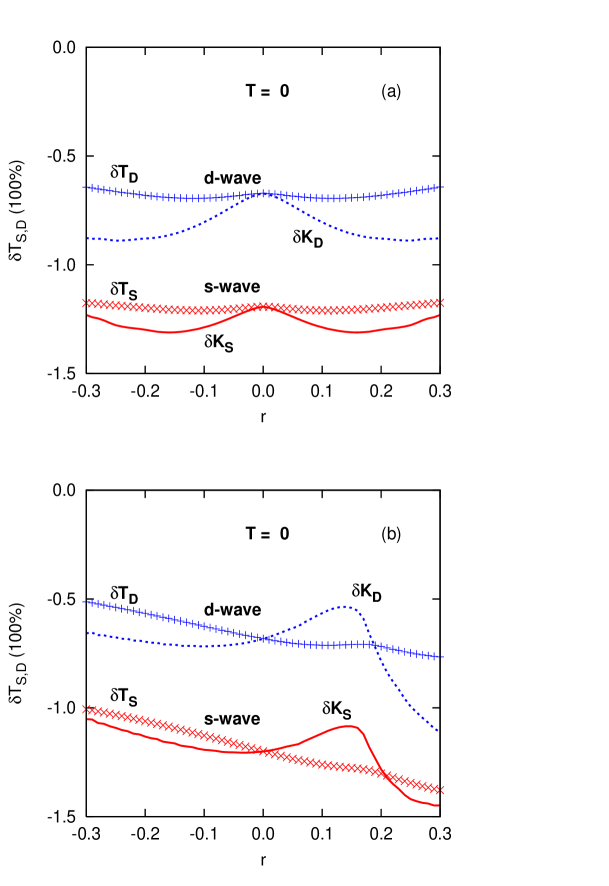
Figure 3: Plot of sum rule difference, Eq. (15) (curves) vs. next-nearest neighbour hopping ($r\equiv t^{\prime}/t$) for (a) half-filling, and (b) $n=0.85$. The symbols are for the corresponding difference in the magnitude of the kinetic energies. They are in good qualitative agreement throughout the range of interest.

IV reversal of kinetic energy change at $T_{c}$

Inspection of Fig. 2 (compare two red, solid curves) makes it clear that a sudden drop in the scattering rate at $T_{c}$ will result in an increase in spectral weight that can more than compensate the decrease due to the opening of a superconductor gap. We simply adopt the phenomenological observation of Hosseini et al. hosseini99 and use the following model for the elastic scattering rate, $\Gamma(T)$:

$$\Gamma(T)=\cases{\Gamma_{0}\phantom{aaaaaaaaaaaa}{\rm for}\phantom{aaaa}T>T_{c},\cr\Gamma_{0}\bigl{(}{T\over T_{c}}\bigr{)}^{4}\phantom{aaaaaaa}{\rm for}\phantom{aaaa}T<T_{c}.}$$ (16)

Note that we could include a linear temperature dependence in the normal state, based on the linear resistivity; this would serve to increase the (negative) slope in Fig. 2, in agreement with observations. However, our attitude has been to adopt this simple model to describe the superconducting state, given that we don’t really understand the normal state, so we will leave this as it is. In the superconducting state, one could include a residual scattering rate due to impurity scattering, as Hosseini et al. hosseini99 have observed, even in their very clean crystals. However, this is a minor effect, and also goes beyond the spirit of the simple phenomenology that we are proposing here.

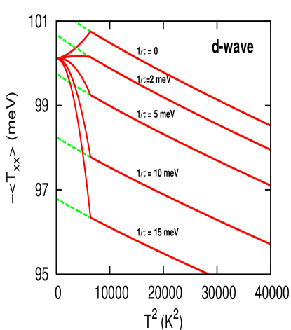
Figure 4: Optical integral (RHS of Eq. (1)) vs. temperature, for various degrees of elastic scattering. Below $T_{c}$ we change the elastic scattering rate smoothly to zero (Eq. (16), as the temperature is lowered. Further details of the calculation are given in the text.

In Fig. 4 we show results for the sum rule with Eq. (16) ”put in by hand”. Since we have assumed that the crystals are completely free of impurities, the end point at zero temperature is the same for all cases shown. It is difficult to try to pin down the amount of inelastic scattering that gets suppressed below $T_{c}$, based on this figure, because we can’t use the normal state result as a benchmark. Our slope is too low in absolute value, and as already mentioned, the normal state is undoubtedly not reasonably described by our simple approach. Nonetheless, it is clear that the amount of inelastic scattering that is suppressed in the superconducting state has to exceed a minimum value so that the sum rule will exhibit anomalous behaviour. As indicated, a small amount of inelastic scattering to begin with (say, less than 2 meV for the parameters used in this figure), does not make up for the decrease expected from conventional BCS theory.

V summary

It is clear that Fig. 4 “explains” the anomalous optical sum rule. To be precise it suggests that the origin of this anomaly is the same mechanism that leads to the large coherence peak in the microwave hosseini99 and to the other observations of sharply increased coherence in the superconducting state johnson05 . It is another matter, however, to claim that this increased coherence is an intrinsic part of the mechanism. To our knowledge the hole mechanism hirsch89 ; hirsch89a is the only mechanism for which this is the case in the plane. In other models, the increased coherence generally arises due to a freezing of the scattering mechanism, as originally suggested by Nuss et al. nuss91, . Fig. 4 also indicates a source of non-universal behaviour. If, for some materials or doping levels the loss in inelastic scattering is small compared to the gap value, then more conventional behaviour of the sum rule (eg. the uppermost curve in Fig. 4) will prevail.

The virtue of this work is its simplicity. Without knowing the details of the inelastic scattering process whose disappearance in the superconducting state is responsible for a sharply decreased scattering rate, we are able to understand the sum rule anomaly. Of course this immediately implies correlations among the various experiments. For example, should the anomaly not be present in overdoped samples, then the microwave peak and neutron scattering resonance should also be absent. Impurities should mask the effect, since they presumably impact the superconducting state as well as the normal state remark , so it is important to have very clean samples. We have adopted the $T^{4}$ dependence for the scattering rate suggested in Ref. hosseini99, , but the qualitative anomaly will not depend on the detailed temperature dependence, but rather on the overall magnitude of the change in effective scattering rate.

- (1) A. Kaminski, J. Mesot, H.M. Fretwell, J.C. Campuzano, M.R. Norman, M. Randeria, H. Ding, T. Sato, T. Takahashi, T. Mochiku, K. Kadowaki, and H. Hoechst, Phys. Rev. Lett. 84, 1788 (2000).
- (2) M. Chiao, R.W. Hill, C. Lupien, L. Taillefer, P. Lambert, R. Gagnon, and P. Fournier, Phys. Rev. B62, 3554 (2000).
- (3) R. Kubo, J. Phys. Soc. Japan 12, 570 (1957).
- (4) D.N. Basov, S.I. Woods, A.S. Katz, E.J. Singley, R.C. Dynes, M. Xu, D.G. Hinks, C.C. Homes, and M. Strongin, Science 283, 49 (1999); A.S. Katz, S.I. Woods, E.J. Singley, T. W. Li, M. Xu, D.G. Hinks, R.C. Dynes and D.N. Basov, Phys. Rev. B61, 5930 (2000).
- (5) H.J.A. Molegraaf, C. Presura, D. van der Marel, P.H. Kes, and M. Li, Science 295, 2239 (2002).
- (6) A.F. Santander-Syro, R.P.S.M. Lobo, N. Bontemps, Z. Konstantinovic, Z.Z. Li, H. Raffy, Europhys. Lett. 62, 568 (2003); A.F. Santander-Syro, R.P.S.M. Lobo, N. Bontemps, W. Lopera, D. Girata, Z. Konstantinovic, Z.Z. Li, H. Raffy, Phys. Rev. B 70, 134504 (2004).
- (7) A.V. Boris, N.N. Kovaleva, O.V. Dolgov, T. Holden, C.T. Lin, B. Keimer, C. Bernhard, Science 304, 708 (2004).
- (8) A.B. Kuzmenko, H.J.A. Molegraaf, F. Carbone, D. van der Marel, cond-mat/0503768.
- (9) A. F. Santander-Syro, N. Bontemps, cond-mat/0503767.
- (10) P.F. Maldague, Phys. Rev. B16, 2437 (1977).
- (11) J.E. Hirsch and F. Marsiglio, Physica C 331, 150 (2000); J.E. Hirsch and F. Marsiglio, Phys. Rev. B62, 15131 (2000).
- (12) M.R. Norman and C. Pépin, Phys. Rev. B 66, 100506 (2002).
- (13) D. van der Marel, H.J.A. Molegraaf, C. Presura, and I. Santoso, in Concepts in Electron Correlations, edited by A. Hewson and V. Zlatic (Kluwer, 2003). See also cond-mat/0302169.
- (14) L. Benfatto, S. G. Sharapov, N. Andrenacci, and H. Beck, Phys. Rev. B 71, 104511 (2005).
- (15) F. Carbone, A.B. Kuzmenko, H.J.A. Molegraaf, E. van Heumen, E. Giannini, D. van der Marel, preprint 2005.
- (16) J.E. Hirsch, Physica C 199, 305 (1992); Physica C 201, 347 (1992).
- (17) J.E. Hirsch, Phys. Lett. A134, 451 (1989).
- (18) J.E. Hirsch and F. Marsiglio, Phys. Rev. B39, 11515 (1989).
- (19) A. Knigavko, J. P. Carbotte, and F. Marsiglio, Phys. Rev. B 70, 224501 (2004).
- (20) E. Schachinger and J. P. Carbotte, Phys. Rev. B 72, 014535 (2005).
- (21) A. Kaminski, M. Randeria, J.C. Campuzano, M. R. Norman, H. Fretwell, J. Mesot, T. Sato, T. Takahashi, and K. Kadowaki, Phys. Rev. Lett. 86, 1070 (2001).
- (22) J. Rossat-Mignod et al., Physica (Amsterdam) 185C-189C, 86 (1991).
- (23) A. Hosseini, R. Harris, S. Kamal, P. Dosanjh, J. Preston, R. Liang, W.N. Hardy, and D.A. Bonn, Phys. Rev. B 60, 1349 (1999).
- (24) D.A. Bonn, P. Dosanjh, R. Liang, and W.N. Hardy, Phys. Rev. Lett. 68, 2390 (1992).
- (25) M.C. Nuss, P.M. Mankiewich, M.L. O Malley, E.H. Westerwick, and P.B. Littlewood, Phys. Rev. Lett. 66, 3305 (1991).
- (26) J.R. Schrieffer, Theory of Superconductivity (Benjamin/Cummings, Don Mills, 1964).
- (27) P. Johnson, private communication.
- (28) Note that even in the case of an s-wave order parameter, the impurity scattering is still present in the superconducting state, and so the optical sum rule behaves as illustrated in Fig. 2. Impurities become “invisible” in the superconducting state only for some properties (like , or the density of states), but not for the kinetic energy.