Velocity Selection in 3D Dendrites:
Phase Field Computations and Microgravity Experiments

Abstract

The growth of a single needle of succinonitrile (SCN) is studied in three dimensional space by using a phase field model. For realistic physical parameters, namely, the large differences in the length scales, i.e., the capillarity length ($10^{-8}{cm}$ - $10^{-6}{cm}$), the radius of the curvature at the tip of the interface (${10^{-3}}{cm}$ - ${10^{-2}}{~{}cm}$) and the diffusion length (${10^{-3}}{cm}$ - $10^{-1}{cm}$), resolution of the large differences in length scale necessitates a $500^{3}$ grid on the supercomputer. The parameters, initial and boundary conditions used are identical to those of the microgravity experiments of Glicksman et al for SCN. The numerical results for the tip velocity are (i) largely consistent with the Space Shuttle experiments; (ii) compatible with the experimental conclusion that tip velocity does not increase with increased anisotropy; (iii) different for 2D versus 3D by a factor of approximately $1.9$; (iv) essentially identical for fully versus rotationally symmetric 3D.

1 Introduction

The temporal evolution of an interface during solidification has been under intensive study by physicists and material scientists for several decades. The interface velocity and shape have important consequences for practical metallurgy, as well as the theory, e.g., velocity selection mechanism and nonlinear theory of interfaces.

The simplest observed microstructure is the single needle crystal or dendrite, which is observed to be a shape resembling a paraboloid (but not fully rotationally invariant away from the tip) growing at a constant velocity, $v_{0}$, with tip radius, $R_{0}$.

An early model of this phenomenon by Ivantsov [1] stipulated the heat diffusion equation in one of the phases and imposed latent heat considerations at the interface. With the interface assumed to be at the melting temperature, the absence of an additional length scale implies the existence of an infinite spectrum of pairs of velocities and tip radii, $(v_{0},R_{0})$. Since the experimental results have shown that there is a unique pair $(v_{0},R_{0})$ that is independent of initial conditions, there has been considerable activity toward uncovering the theoretical mechanism for this velocity selection (see, for example [2, 3, 4, 5]). The emergence of the capillarity length associated with the surface tension as an additional length scale has provided an explanation for the selection mechanism. Advances in computational power and a better understanding of interface models and their computation have opened up the possibility of comparing experimental values for the tip velocity with the numerical computations. This is nevertheless a difficult computational issue in part due to the large differences in length scales that range from $1~{}cm$ for the size of the experimental region, to $14$ microns for the radius of curvature near the tip, $10^{-6}{~{}cm}$ for the capillarity length, to $10^{-8}{~{}cm}$ interface thickness length.

One perspective into the theoretical and numerical study of such interfaces has been provided by the phase field model introduced in [6, 7] in which a phase, or order parameter, $\varphi$, and temperature, $T$, are coupled through a pair of partial differential equations described below (see also more recent papers [8, 9, 10]). In physical terms, the width of the transition region exhibited by $\varphi$ is Angstroms. In the $1980$’s three key results facilitated the use of these equations for computation of physical phenomena. If the equations are properly scaled one can (i) identify each of the physical parameters, such as the surface tension, (ii) and attain the sharp interface problem as a limit [11], and (iii) use the interface thickness, $\varepsilon,$ as a free parameter, since the motion of the interface is independent of this parameter  [12]. This last result thereby opened the door to computations with realistic material parameters, by removing the issue of small interface thickness. However, the difference in scale between the radius of the curvature and overall dimensions still pose a computational challenge. More recently, several computations, have been done using the phase field model [13, 14, 15, 16, 17, 18], with some 3D computations in [14] utilizing the model and asymptotics of [19], that will be compared with our results below. Also, George et al studied the simulation of dendritic growth in three dimensional space using a phase field model [20].

Our work differs from the works referenced above in many aspects. However, the main difference arises from the adaptation of the experimental conditions in the simulation of dendritic growth. Most importantly, we use true values of physical parameters which are obtained from the microgravity experiment for SCN [21]. In order to deal with different length scales and the diffusion during freezing in the thin interfacial region, we implement a fully parallel architecture in a three dimensional space which enables us to use enough grid points and perform an efficient calculation.

Solidification is a complicated nonlinear process. Modeling necessarily involves making choices of physical effects that are to be included in the equations. Comparison of computations with experiments that are closest to the mathematical model yields the most convincing test of the model and computations. The modeling of single-needle dendrites has usually been carried out using the diffusion equation as a mechanism for the dissipation of heat. However, all of the experiments until the Space Shuttle experiments had been done under conditions of normal gravity, so that convection in the liquid is an important mechanism for the dissipation of the latent heat released at the interface. The microgravity experiments performed on the Space Shuttle [21] provide the first opportunity to test whether the mathematical models agree with experiments, since the absence of gravity essentially eliminates convection, thereby leaving diffusion as the main mechanism for heat transport away from the interface.

While numerous computer calculations have been performed on both sharp interface and phase field models of solidification, comparison with experiment has always been a difficulty due to the vastly different length scales in the problem (e.g 10${}^{-6}{~{}cm}$ for capillarity length and $1~{}cm$ for the overall dimensions of the experiment), and the three dimensional nature of the problem. In the absence of direct comparison with experiment, it is also difficult to know whether some of the simplifications that have been used, such as setting the kinetic coefficient, $\alpha$, to zero are valid.

In this paper we perform large scale 3D parallel computations of a phase field model with the modification introduced in  [19]. The key aspects of these computations are summarized below.

(A) We perform fully three dimensional parallel computations by adopting the experimental conditions used in the Space Shuttle experiment. The symmetry is utilized only along the major axes (rather than rotational symmetry). This allows us to compare the tip velocity with the actual experiments in a meaningful way. The calculations utilize the parameters and boundary conditions of the IDGE microgravity experiments for SCN [21, 22]. All previous experiments done under normal gravity conditions introduced convection. Hence this provides an opportunity to compare experiments in the absence of convection to theory that also excludes convection. The difference between the experimental results and our computations thereby defines the challenges for additional physical effects that need to be modeled.

(B) The role of anisotropy in velocity selection has been noted in the computational references cited above. Glicksman and Singh [23] compare experimental tip velocity of SCN with pivalic acid (PVA) whose coefficient of surface tension anisotropy (defined below) differs by a factor of $10$ but are otherwise similar, except perhaps for the kinetic coefficient. We perform two sets of calculations in which all parameters are identical (SCN values) except for the anisotropy coefficient. Our computations confirm (consistent with the experimental results [21]) that the velocity is nearly identical when the magnitude of the anisotropy is varied by a factor of $10$ with all other parameters fixed (at the SCN values).

(C) Most of the previous numerical computations that simulate the interface growth were done in two dimensional space. Our computations shows that the 2D and 3D computations differ by a factor of approximately $1.9$. The results of the 3D for tip velocity can also be compared with our previous computations [24] that utilized rotational symmetry to reduce the 3D computations to two computational spatial dimensions.

(D) The role of the kinetic coefficient [see definition of $\alpha$ below equation (2)] is subtle, and this material parameter is often set to zero, for convenience, in theoretical and computational studies. We find, however, that there is a significant difference in the tip velocity when all other parameters are held fixed while this coefficient is varied. Consequently, this kinetic coefficient may be of crucial importance in determining the selection of tip velocity. A better understanding of this issue may lead to theory that can explain a broader range of undercooling and velocity.

2 Mathematical Modeling

In the computations below, we use a version of the phase field equations introduced in [19], for which the phase or order parameter, $\varphi(\vec{x},t)$, as a function of spacial point, $\vec{x}$, and time, $t$, is exactly $-1$ in the solid and $+1$ in the liquid. The order parameter is coupled with the dimensionless temperature, $u$, which is given by the following relation along with the capillary length, $d_{0}$.

$$u(x,t)=\frac{T-T_{m}}{l_{v}/c_{v}},~{}~{}d_{0}=\frac{\sigma c_{v}}{[s]_{E}l_{v}}$$ (1)

where $T_{m}$, $l_{v}$, $c_{v}$, $\sigma$ and $[s]_{E}$ are the melting temperature, latent heat, specific heat per unit volume of the material, surface tension and the difference in the entropy (in equilibrium) per unit volume between the solid phase and liquid phase, respectively. Thus, we can define the interface by $\Gamma=\{x\in\Omega:\varphi(x,t)=0\}$ and write the dimensionless phase field equations as follows

$$\alpha\varepsilon^{2}\varphi_{t}=\varepsilon^{2}\Delta{\varphi}+g(\varphi)+\frac{5}{8}\frac{\varepsilon}{d_{0}}{u}{f^{\prime}(\varphi)}$$ (2)

$$u_{t}+\frac{1}{2}\varphi_{t}=D\Delta{u}$$ (3)

where

$$g(\varphi)=\frac{\varphi-\varphi^{3}}{2},~{}~{}f^{\prime}(\varphi)=(1-\varphi^{2})^{2},~{}~{}D=\frac{K}{c_{v}}$$ (4)

Here, $\alpha$ is the kinetic coefficient and $\varepsilon$ is the interface thickness that can be used as a ”free parameter” [12]. In the limit as $\varepsilon$ vanishes as all other parameters held fixed, solutions to (2) and (3) are governed by the sharp interface model

$$u_{t}=\nabla\cdot D\nabla u$$ (5)

$$v_{n}=-D\left[{\nabla u\cdot\hat{n}}\right]_{-}^{+}$$ (6)

$$u=-d_{0}(\kappa+\alpha v_{n})$$ (7)

where the parameters $d_{0}$, $D$ and $\alpha$ are the same as in the phase field model, and $v_{n}$ is the interface normal growth velocity (with normal $\hat{n}$ chosen from solid ($-$) to liquid ($+$) ) [7, 19].

2.1 Initial and boundary conditions

In order to simulate interface growth of a dendrite in 3D, we choose a cube of ${[-1,1]}^{3}$ which is assumed to be filled with pure SCN melt initially. The solidification of the melt is initiated by a small solid SCN ball of radius, $R_{0}$, which is placed at the center of the chamber. The temperature at the boundary is kept at constant undercooling value, $u_{\infty}$, and the liquid temperature inside the chamber declines exponentially from $u=u_{solid}$ on the interface of the seed to the boundary of the chamber. In particular, the initial conditions of $u$ inside the chamber are given by a plane wave solution to (5) and (6) which is given by

$$u_{trav}(z,t)=\left\{\begin{array}[]{cl}u_{\infty}[1-e^{-v(z-vt/|u_{\infty}|)/(D|u_{\infty}|)}],&z\geq vt/|u_{\infty}|\\ 0,&z<vt/|u_{\infty}|\end{array}\right.$$ (8)

where $z$ is the signed distance from the seed interface (positive in the liquid) and $u_{\infty}=\frac{T_{\infty}-T_{m}}{l_{v}/c_{v}}$ denotes the dimensionless undercooling value where $T_{\infty}$ is the far field temperature. The initial value of $\varphi$ is obtained from a leading term asymptotic expansion solution [19]

$$\varphi(x,t)=\tanh{\left(\frac{z-vt}{2\varepsilon}\right)}+\textit{higher order terms}$$ (9)

2.2 Implementation of anisotropy

Anisotropy is important in determining the shape of dendrites that grow exclusively in the preferred directions. The experimental evidence shows conclusively that surface tension, $\sigma$, exhibits anisotropy [23]. While there is the possibility of dynamical (i.e., through $\alpha$ in equation  (2) or (3)) or other anisotropy the experimental measurements of anisotropy in these experiments are confined to those related to surface tension. Surface tension anisotropy has been modeled in several ways.

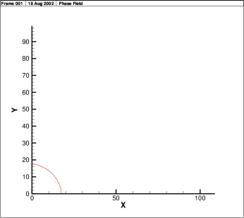
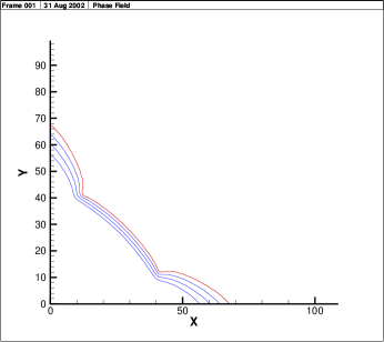
Figure 1: Contour plots of the interface at different times on xy plane for $u_{\infty}=0.0265$ which shows the effect of the anisotropy: (a) The position of the interface in 10 seconds; (b) The position of the interface at latter times (135 sec, 140 sec, 145 sec and 150 sec).

Let $\hat{n}=(n_{x},n_{y},n_{z})$ be the normal to the interface. We utilize the simplest possible function describing the dependence of surface energy on $\hat{n}$ in the case of an underlying cubic symmetry. The relation can be given by [25, 26]

$$\sigma(\hat{n})=a_{s}[1+{\epsilon}^{\prime}(n_{x}^{4}+n_{y}^{4}+n_{z}^{4})]$$ (10)

which is rewritten in terms of spherical angles as

$$\gamma(\theta,\phi)=a_{s}\{1+\zeta[\cos^{4}{\phi}+\sin^{4}{\phi}(1-2\sin^{2}{\theta}\cos^{2}{\theta})]\}$$ (11)

where $\theta$ and $\phi$ are the angles which correspond to the normal, $n$, with respect to a crystal axis. The parameters, $\zeta$ and $a_{s}$, can be related to usual measure of anisotropy strength, $\delta_{\sigma}$, by the relations $a_{s}=(1-3{\delta_{\sigma}})$ and $\zeta=\frac{4\delta_{\sigma}}{a_{s}}$ [14].

Aysmptotic analysis [27] shows that with the anisotropy, the Gibbs-Thomson relation (7) is modified not only in terms of the angles, but with their second derivatives. In our simulation, we assume that the dendrites grow along an axis of symmetry and set $\kappa$ to be the mean curvature. Thus, we can rewrite the Gibbs-Thomson equation (7) as

$$u=-~{}\overline{d}_{0}(\hat{n})\kappa-\overline{d}_{0}(\hat{n}){\alpha}v_{n}$$ (12)

where

$$\overline{d}_{0}(\theta,\phi)=d_{0}[\gamma(\theta,\phi)+\frac{\partial^{2}\gamma(\theta,\phi)}{\partial{\theta}^{2}}+\frac{\partial^{2}\gamma(\theta,\phi)}{\partial{\phi}^{2}}]$$ (13)

3 Discretization

A large number of mesh points are necessary in order to calculate the tip growth velocity and tip radius accurately. The values of $u$ and $\varphi$ across the interface vary from maximum to minimum within a short distance. This requires finer grid spacing so that number of mesh points is adequate to resolve the interfacial area. We make a physically reasonable but computationally very useful assumption that the dendrite grows symmetrically along the coordinate axes. Thus, the computational domain is reduced to $\Omega=[0,1]^{3}$ which decreases the overall grid usage by $7/8$. In this work, we use $400\--500$ uniform grid points on each side of $\Omega$ which guarantees that we have at least $6$-$7$ grid points located on the interface region as measured from $\varphi=-0.9$ to $\varphi=0.9$.

In order to discretize the equations (2) and (3), let $\varphi^{p}_{ijk}$ and $u^{p}_{ijk}$ denote the discrete values of $\varphi(x_{i},y_{j},z_{k},t_{p})$ and $u(x_{i},y_{j},z_{k},t_{p})$, respectively. We lag the nonlinear terms in (2) and discretize the equations (2) and (3) by using semi-implicit Crank-Nicolson finite difference method. Thus, we write the discrete equations as follows:

$$\delta_{t}^{+}u_{ijk}^{p}=\frac{D}{2}\{\Delta{u}^{p}_{ijk}+\Delta{u}^{p+1}_{ijk}\}-\frac{1}{2}\delta_{t}^{+}\varphi_{ijk}^{p}$$ (14)

$$\varepsilon^{2}\alpha\delta_{t}^{+}\varphi_{ijk}^{p}=\frac{\varepsilon^{2}}{2}\{\Delta{\varphi}^{p}_{ijk}+\Delta{\varphi}^{p+1}_{ijk}\}+g(\varphi_{ijk}^{p})+\frac{5}{8}\frac{\varepsilon}{d_{0}}u_{ijk}^{p}f^{\prime}(\varphi_{ijk}^{p})$$ (15)

where

$$\Delta{\phi^{T}_{ijk}}=\delta^{\pm}_{x_{i}}\phi_{ijk}^{T}+\delta^{\pm}_{y_{j}}\phi_{ijk}^{T}+\delta^{\pm}_{z_{k}}\phi_{ijk}^{T}$$ (16)

for $i,j,k=0,1,2,...,N-1$ and $p=0,1,2,...,T_{final}$. The operators such as $\delta^{\pm}_{x}$ and $\delta_{t}^{+}$ in the equations (14) and (15) are the finite difference operators and they can be given as

$$\delta_{x}^{\pm}\phi(x,y,z,t)=\frac{\phi(x+\Delta{x},y,z,t)+\phi(x-\Delta{x},y,z,t)-2\phi(x,y,z,t)}{(\Delta{x})^{2}}$$ (17)

and

$$\delta_{t}^{+}\phi(x,y,z,t)=\frac{\phi(x,y,z,t+\Delta{t})-\phi(x,y,z,t)}{\Delta{t}}\cdot$$ (18)

4 Values of SCN Parameters

The comparison of the computational results with experiments makes sense only if we use the true value of the physical parameters. Throughout the simulation, the parameters $d_{0}$ and $\sigma_{0}$ for SCN are set to be $2.83\times 10^{-7}~{}cm$ and $8.9~{}ergs/cm^{2}$, respectively [22]. The diffusivity parameters, $D_{liquid}$ and $D_{solid}$, are almost the same for the liquid and solid SCN. Thus, we set the diffusivity $D$ to be $1.147\times 10^{-3}cm^{2}/sec$ which is the value for $D_{liquid}$ [22].

All of the parameters in the phase field equations are physically measurable quantities, including $\varepsilon$ which is a measure of the interface thickness. It was shown in [7, 11] that the solutions of the phase field equations (scaled in this form) approach those of the sharp interface model (5)-(7) provided all other parameters are held fixed as $\varepsilon$ approaches zero. The rate of convergence, however, emerges as a key issue. In particular, the true size of $\varepsilon$ is a few atomic lengths, or Angstrom, while the size of experimental region is at least $1cm$. Thus using the true value of $\varepsilon$ would necessitate $10^{9}$ grid points in each direction yielding unfeasible computation. From a computational perspective, one needs to have at least several grid points in the interfacial region in order to accurately calculate the derivatives of order parameter that implicitly define the surface tension.

A computational breakthrough was the discovery that $\varepsilon$ could be made many orders of magnitude larger without influencing the interface motion. Caginalp and Socolovsky [12, 28] showed that so long as one chooses an appropriate number of grid points in the interface region (defined by the magnitude of $\varepsilon$ and $h$ denotes the uniform grid size), guaranteed by the range $0.75<\frac{\varepsilon}{h}<1.1$, one can resolve the motion accurately. The only limitation then involves the interface thickness relative to the radius of curvature of the dendrites. In this work we set $\varepsilon=h$ which falls into this range.

The choice of the initial tip radius, $R_{0}$, for a steady-state is not arbitrary. One needs to take into account the latent heat released at the interface. By choosing a sufficiently large distance between the interface and the boundary, the latent heat released at the interface diffuses to the liquid and the effect of the boundary becomes minimal. In order to guarantee enough distance to the boundary, the tip radius, $R_{0}$, should be at least $20$ times smaller than the diffusion length $D/v_{n}$. In our calculation, we choose the tip radius to be $R_{0}=20{h}$ for the choice of $N=500$ and $R_{0}=14{h}$ for $N=400$ where $h$ is the uniform grid size corresponding to the choice of each $N$. Under these conditions, the diffusion length is large enough and satisfies the standard theoretical conditions for dendritic growth [17].

5 Parallelization and data distribution

The numerical simulation of the equations (2) and (3) in 3D with any physical choice of parameters is a difficult task. Of these difficulties, the memory requirements and the CPU time are the main issues due to the difference in the length scales. As shown in Table 1, the demand for the memory is a delicate issue in that doubling the number of the grids will increase the computational memory as much as eight times, and slows down the performance of the code. This makes the numerical computation of (14) and (15) with any physically appropriate choice of grid size impossible on serial computers. Instead, one needs a parallel architecture in which the work will be distributed to many computers and the computational job will be shared among the computers (processors) allowing large scale computation.

Table 1: Table shows the memory allocation on each processor (of 32 processors) when the number of grid points are doubled.

Grid points	Memory(MB)	Ratio
$32^{3}$	$1.45$	-
$64^{3}$	$10.56$	$7.28$
$128^{3}$	76.90	$7.28$
$216^{3}$	611.03	$7.95$

In this work, we use PETSC’s distributed memory architecture (DA), whose characteristic feature is that each processor owns its own local memory, and memory of other processors can not be accessed directly [29]. The PETSC/DA system requires communication to inquire or borrow information among the processors. In particular for the numerical solution of PDE’s, each processor requires its local portion of the information as well as the points on the boundary of the adjacent processors to update the right hand side vector. The communication required among the processors to exchange the components and points along the border of the adjacent subdomains are managed via the DA system while the actual data is stored in appropriately sized local vector objects. Thus, the DA objects only contain the parallel layout and communication information, and they are not intended for storing the matrices and vectors.

The communication is necessary but it is very critical that the parallel code be designed independent of the other processors as much as possible and the ratio of communication among the processors should be kept small. Otherwise, a high ratio of communications among the processors slows down the computation. Therefore, it is very important that the communication should be limited to the neighboring processors and should avoid global communication if possible. Similarly, the distribution of the work load among the processors is another important issue in parallel computation. In our work, we keep the number of grid points proportional to the number of processor so that each processor is assigned almost the same amount of work load. This enables the efficient use of the processors and makes the processors to work in a synchrony. The Table 2 shows that both the CPU time and memory allocation are almost halved when the number of the processors doubled.

The allocation of memory, creation of the parallel matrices and vectors, and setting up the solver contexts are very time consuming. Therefore, one would like to use the same initial setup through out the computation if possible. This is a good approach especially when the coefficient matrix is independent of time which is the case in this work. Thus, we can use the same coefficient matrices as well as the same preconditioners throughout the calculations.

Parallel solutions of (14) and  (15) are done via the linear solver of PETSC [29] in which we use CG iterative method with Jacobi Preconditioning.

Table 2: The performance of the algorithm is tested for fixed grid (N=128): Table shows the wall-clock time, number of flops and the rate of scalability of the algorithm on different number of processors.

Number of PE	MFlops/s	Memory (MB)	Wall Clock (s)	Ratio
4	50	492.8	1165.78	-
8	52	255.5	574.58	2.00
16	54	136.5	314.15	3.71
32	55	76.9	168.87	6.90
64	53	47.0	88.59	13.15

5.1 Memory allocation and scalability of the algorithm

In the numerical solution of (14) and (15), we allocate memory for six parallel and one sequential global vectors of the size $N^{3}$, and two parallel global matrices of the size $N^{3}\times{N^{3}}$. Together with the creation of the DA system, local vectors and matrices, the memory requirement becomes huge for larger $N$. We verify this in Table 1 by varying the number of grid points. In fact, it shows that as $N$ is doubled, the memory on each processor is increased approximately eight times. Thus as N increases, the demand for the memory gets so large that even for supercomputers such as Lemieux, there are considerable limitations of the number when grid points are larger than $N=600$. As Table 1 indicates, the memory required for a fully three dimensional computation of phase field model is enormous if one wants to use a reasonable number of grid points in the simulation. This necessitates the use of not only high performance computers but also computers which can accommodate the memory needed. One way to over come this difficulty is to use parallel architecture which is the key in our work in handling the memory deficiency.

Table 3: A sufficient grid size for accurate calculation of interphase growth velocities for SCN is examined. The velocities for $u_{\infty}=0.01$ are shown at $t_{final}=16$ sec from the initial stage.

Grid Number	Velocity (cm/sec)
$200$	0.002100
$300$	0.000363
$400$	0.000310
$500$	0.000327
$600$	0.000342
$700$	0.000357

The scalability of the code is a measure by which one can test whether the processors are efficiently used during the computation. For this we fix the number of the grid points at $N=128$ and set $T_{final}=300$. By doubling the number of the processors each time we calculate the corresponding wall-clock time for the same job. As shown in the Table 2 the wall-clock time almost doubles when we halved the number of the processors. This is an indication that the code scales well with the number of the processors.

As it is apparent from above analysis, memory allocation is still a delicate issue which influence the choice of grid size N very much. In our earlier work [24], we studied the grid convergence in $2D$ by comparing the growth velocities for different choice of grid points ranging from $200$ to $700$ when all other parameters kept fixed. Table 3 shows the corresponding velocities for the grid points from $200$ to $700$ when all other conditions are identical for the undercooling value $0.001$. As seen in Table 3, the interface growth velocity does not differ much when we vary the number of grid points, $N$, from $400$ to $700$ indicating that a choice of $N=500$ will be enough to study dendritic growth. In this work, we use $N=500$ in the calculation of undercooling vs. growth velocity linearity relation. For other calculation such as the study of anisotropy and kinetic coefficient, we set $N=400$. Also, the time step $\Delta{t}$ is chosen to be $5\times{10^{-3}}$ throughout the computation.

6 Results and conclusions

In this paper we have performed parallel computations in three-dimensional space with the specific parameters and boundary conditions which are used in the microgravity experimental setup for SCN.

The microgravity experiments exclude most of the convection effects so that computations involving the physics described by equations (2)-(3) or  (5)-(7) can be tested against the experiment. Prior to these experiments, theoretical results and computer calculations were awkward in that theory without convection was tested against experiment (on Earth) with convection. Thus the interpretation of agreement was ambiguous, leaving open the possibility of inaccurate computations on inadequate modeling of experimental setup.

In order to address the questions raised in (A) and (B) of the introduction, we have considered eight different undercooling values, $u_{\infty}$, from the microgravity experiments for SCN [30]. During the simulation we set $R_{0}=20$, $N=500$ and $T_{final}=2000$ and compute the average growth velocity for each undercooling value. The computational and experimental growth velocities for each undercooling are given in the Table 4.

Table 4: Table shows the computational and experimental interface growth velocity for several SCN undercooling values in terms of (cm/sec). First two columns contain SCN undercooling values and the corresponding growth velocities from space shuttle experiments, respectively. The computational results from parallel computing and 3D computation under the rotational symmetry are given in third and fourth columns.

$u_{\infty}$	Microgravity Vel.	Rot.Symmet.Vel.	Parallel Vel.
0.04370	0.016980	0.001770	0.001840
0.03380	0.008720	0.001486	0.001480
0.02650	0.004620	0.001273	0.001370
0.02050	0.002328	0.001066	0.001068
0.01610	0.001417	0.000922	0.000902
0.01260	0.000840	0.000784	0.000756
0.01000	0.000500	0.000681	0.000626
0.00790	0.000343	0.000590	0.000456

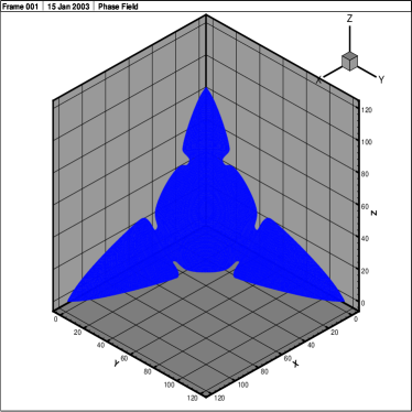
Figure 2: SCN dendrite at $u_{\infty}=0.0265$,  after $215$ seconds: (a) Projection of 3D dendrite on $xy$ plane; (b) 3D SCN dendrite in the first octant.

The results in Table 4 and corresponding Fig 3 show that computational velocity is consistent with other 3D phase field computations (see e.g. [24]). The overall results are close to the experiments, particularly for undercooling temperatures that are neither very small nor very large. In particular, since solidification is a complicated process, it is likely that many other physical effects play a role in determining the growth velocity at the tip of the dendrite  [31]. The equations (5)-(7) or equivalently (2) and (3) incorporate all of the physics that have generally been used to study these problems. Furthermore the numerical schemes are also known to be reliable through various checks. Hence, it appears that the difference between our computations and microgravity experiments can be attributed to additional physics that is not part of the standard models such as (5) and (6). For the intermediate values of, such as $0.0126$, the difference is negligible. Thus, it appears that the model (equations (2) and (3)) includes the key physical components necessary to describe the solidification process within this undercooling regime. In particular, undercoolings that are at the extremes of experimental range, it is quite likely that simplest physical description given by  (5), (6), neglects physical factors that are significant in terms of the growth velocity. At the low end, this might include, for example, adsorption. At the high end of undercooling, which generates the higher velocities, the motion of the dendrite is likely to produce some convective distribution of heat that would differ from pure heat diffusion in the liquid. This may be one of the source of randomness or noise that leads to extensive sidebranching which would lead to additional corrections to the velocity. At the present there are no coherent methods to incorporate noise into the phase field (or sharp interface) equations. In the absence of experimental data on interface noise, the use of noise in computations would involve at least two ad hoc parameters (amplitude and frequency), so that any resulting agreement with the experimental data would not be very meaningful.

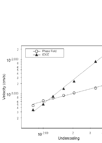
Figure 3: Figure confirms the theoretical result that there is a linear relation between the undercooling and computational growth velocity ($u_{\infty}=0.0265$).

The model includes several features such as surface tension and kinetic undercooling. The importance of surface tension (manifested in the capillarity length, $d_{0}$) has been noted in studies of linear stability [32, 33] and computations. However, the kinetic undercooling, $\alpha$, is often neglected in computations and theoretical studies. In fact, while the phase field equations naturally incorporate this material parameter, some calculations have used a limit in which $\alpha$ approaches zero, rather than its true value, for computational convenience. We perform pairs of calculations for the undercooling value $0.0205$ in which all parameters were identical except for $\alpha$ (see Table 5).

Table 5: Table shows the effect of kinetic coefficient on the growth velocity of interface for the undercooling $u_{\infty}=0.0205$.

$\alpha(sec/cm^{2})$	Velocity(cm/sec)
2.5x$10^{6}$	0.00117
3.5x$10^{6}$	0.00090
5.0x$10^{6}$	0.00106

These results indicate that a change in the kinetic coefficient of 28.5% can result in a growth velocity that is 30% as shown in Table 5. This suggests that $\alpha$ ( as $\beta:={\alpha}d_{0}$ as the computation of the velocity in Gibbs- Thomson relation (7)) can not be used as a free parameter, as can $\varepsilon$, the interface thickness. Moreover, variation in $\alpha$ implies a change in growth velocity, as does a variation in any of the other parameters such as $c_{v}$, $l_{v}$, $K$, $etc.$. In all other computations, we set $\alpha$ to be $3.5\times{10^{6}}sec/{cm^{2}}$ which is approximated by using SCN microgravity values in (7).

Our results have some interesting implications for dimensionality, as we can compare our 3D calculations to 2D calculations and to rotationally symmetric 3D calculations in which we used cylindrical coordinates and assumed that the dependence was purely radial. The experimental pictures indicate that the cylindrical symmetry of the single-needle crystal breaks down shortly beyond the tip. Our results, however, indicate that there is relatively little difference in velocity between the two calculations. The tip velocity calculations in 3D and 2D, on the other hand, differ by about a factor of $1.9$ (see Table 6).

Table 6: The table shows the computational interface growth velocities (cm/sec) in $2D$ and 3D (parallel) for different undercooling values.

Undercooling	2D-Velocity	3D-Velocity
0.01	0.00033	0.00063
0.0161	0.00050	0.00090
0.0265	0.00066	0.00137

The ratio $1.9$ can be put in perspective by examining the limiting sharp interface equations (5) and (6). Physical intuition suggests that the growth of the interface is limited mainly by the diffusion of the latent heat manifested in the condition (6). When diffusion is rapid, the heat equation is approximated by Laplace’s equation, whose radial solutions are of the form $r^{d}$. The latent heat condition (6) implies that the normal velocity is proportional to the gradient, or $dr^{d-1}$. Comparing this term for $d=3$ versus $d=2$, one has a ratio of $3/2=1.5$. Analogously, if we examine the Gibbs-Thomson relation alone, and solve (7) for the normal velocity, we see that dimensionality arises (directly) in terms of $k$, the sum of principal curvatures, which is $(d-1)/R_{0}$ where $R_{0}$ is the radius of curvature. Hence this factor would suggest that at least one of the terms in this expression for the velocity has a coefficient $d-1$, suggesting a ratio of $(3-1)/(2-1)=2$. Thus a heuristic examination of the key limiting equations suggests that the tip velocity in $3D$ should be about $1.5$ to $2$ times that of the $2D$ system. Of course there are numerous nonlinearities involved in the equations that could alter this ratio. Our calculations fall well in the range $1.5$ to $2$, thereby lending some support to the heuristics above.

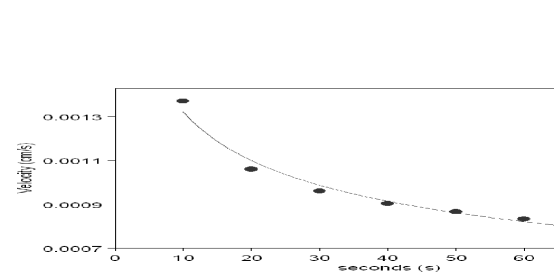
Figure 4: Figure confirms the theoretical result that the growth velocity approaches a constant value in large time ($u_{\infty}=0.0265$).

The fully three dimensional calculations also allow a complete treatment of the anisotropy as it is manifested in both directions (see equation 10). While the immediate area near the tip of the dendrite appears to be symmetric about the direction of growth, the photographs of experiments show that there is significant asymmetry a short distance away from the tip. Consequently, there is some question as to the accuracy of rotationally symmetric computations (reducing the 3D problem to one which is a 2D computation). However, we find that this asymmetry influences the tip velocity by only 8-10%. Nevertheless this anisotropy can be expected to play a key role in the development of sidebranching for which the axial symmetry appears to be significant.

To verify the effect of the surface tension anisotropy on the interface growth, we use four different anisotropy levels, $0.00$,  $0.006$,  $0.009$  and  $0.01$ for the undercooling value $0.0205$. Corresponding growth velocities are $9.1\times 10^{-4}~{}cm/sec$, $1.16\times 10^{-3}cm/sec$,  $1.20\times 10^{-3}cm/sec$ and $1.07\times 10^{-3}cm/sec$, respectively. The influence of the anisotropy on the shape of the interface is more clear compared to the effects on the growth velocity(see Fig 1). An order of magnitude change in the anisotropy strength does not change tip velocity significantly which confirm the experimental result [23] as well as the results from rotational symmetry case we studied in [24]. We also observe that the tip of the interface becomes sharper in the preferred direction as the strength of the anisotropy increases.

As indicated in experiments, theory and computational studies [9], the average growth rate of a single needle-crystal in 3D approaches a constant value. We examine this issue by using the undercooling value, $u_{\infty}=0.0205$, for SCN. The average growth velocities at different time steps are calculated with the anisotropy strength $\delta_{\sigma}=0.01$. The growth velocity approaches a constant value as $T_{final}$ gets larger (see Fig 4) which confirms previous computational and theoretical studies [9].

We have performed all of our calculations on the terascale computing system, Lemieux, at Pittsburgh Super Computing Center. Lemieux consists of $750$ Compaq Alphaserver $ES45$ nodes and two separate front end nodes. Each node contains four 1-GHz processors SMP with $4$ Gbytes of memory.

References

- [1] G. P. Ivantsov, Dokl.Akad.Nauk USSR, 58, 1947, pp. 567
- [2] Ben-Jacob and N. Goldenfeld and B. Kotliar and J. Langer, Phys. Rev. Lett. 53, 1984
- [3] D. A. Kessler and J. Koplik and H. Levine, Phys. Rev. A, 30, 1984, pp. 3161; Adv. Phys,37, 1988, pp. 255
- [4] E. Brener and V. I. Melnikov, Adv. Phys, 40, 1991, pp. 53
- [5] Y. Pomeau and M. B. Amar, Cambridge Univ. Press, Cambr. England, 1991
- [6] G. Caginalp, Carnegie Mellon Research Report, Pittsburgh, 1982
- [7] G. Caginalp, Lecture Notes, Springer, Berlin, 1984
- [8] R. Almgren, SIAM J. Appl.Math, 59, 1999, 2086
- [9] Y. Kim and N. Provatas and N. Goldenfeld and J. Dantzig, Phys. Rev. E, 59, 1999, 2546
- [10] S. Hariharan and G. W. Young, SIAM J.Appl.Math, 62, 2001, 244
- [11] G. Caginalp, Archive for Rational Mechanics and Analysis, 92, 1986, 203
- [12] G. Caginalp and E. A. Socolovsky, Appl.Math.Lett, 2, 1989, 117
- [13] T. Abel and E. Brener and H. M. Krumbhaar, Phys Rev E, 55, 1997, 7789-7792
- [14] A. Karma and W-J. Rappel, Phys. Rev. E, 57, 1998, 4323
- [15] J. A. Warner and R. Kobayashi and W. C. Carter, J. Cyrstal Growth, 211, 2000
- [16] L. L. Regel and W. R. Wilcox and D. Popov and F. C. Li, Acta astronautica, 48, 2001, 101-108
- [17] N. Provatas and N. Goldenfeld and J. Dantzig and J. C. LaCombe and A. Lupelescu and M. B. Koss and M. E. Glicksman and R. Almgren, Phys. Rev. Lett., 82, 1999, 4496-4499
- [18] S. L. Wang and R. F. Sekerka and A. A. Wheeler and B. F. Murray and S. R. Corriell and J. Brown and G. B. McFadden, Physica D, 69, 1993, 189-200
- [19] G. Caginalp and X. Chen, Springer, New York, 43, 1991, 1-28
- [20] W. L. George and J. A. Warren, J. Compuatational Physics, 177, 2002, 264-283
- [21] M. B. Koss and M. E. Glicksman and L. T. Bushnell and J. C. LaCombe and E. A. Winsa, ISIJ, 35, 1995, 604
- [22] M. E. Glicksman and R.J. Schaefer and J.D. Ayers, Met. Mat. Trans., A7, 1977, 1747-1759
- [23] M. E. Glicksman and N. B. Singh, J. Cyrstal Growth, 98, 1989, 207
- [24] Y. B. Altundas and G. Caginalp, J. Statistical Physics, 110, 2003, 1055-1066
- [25] D. A. Kessler and H. Levine, Adv. Phys, 37, 1988, 255
- [26] A. A. Wheeler and G. B. McFadden, Proc. R. Soc. London, 453A, 1997, 1611
- [27] G. Caginalp, Ann. Phys, 172, 1986, 136-155
- [28] G. Caginalp and E. A. Socolovsky, J. Computational Physics, 95, 1991, 85-100
- [29] S. Balay and W. D. Gropp and L. C. McInnes and B. F. Smith, 163–202, Birkhauser Press, 1997
- [30] M. E. Glicksman and M.B. Koss and E. A. Winsa, Phys. Rev. Lett., 73, 1994, 573
- [31] W. A. Tiller and K. A. Jackson and J. W. Rutter and B. Chalmers, Acta Metalurgica, 1, 1953, 428
- [32] J. Ockendon, Free boundary problems (Proc. Pavia Conference, E. Magens Ed.), Bologna,1980
- [33] W. W. Mullins and R. F. Sekerka, J. Appl. Phys. 34, 1963, 323-329