Complex networks generated by the Penna bit-string model: Emergence of small-world and assortative mixing

Abstract

The Penna bit-string model successfully encompasses many phenomena of population evolution, including inheritance, mutation, evolution and ageing. If we consider social interactions among individuals in the Penna model, the population will form a complex network. In this paper, we first modify the Verhulst factor to control only the birth rate, and introduce activity-based preferential reproduction of offspring in the Penna model. The social interactions among individuals are generated by both inheritance and activity-based preferential increase. Then we study the properties of the complex network generated by the modified Penna model. We find that the resulting complex network has a small-world effect and the assortative mixing property.

In recent years, the usage of computational models has turned into a major trend in the discussion of problems in population dynamics and evolutionary theory. In 1995, a bit-string computer simulation model for population evolution was introduced by Penna [1], which encompasses the inheritance, mutation, evolution and ageing phenomena. The Penna model has been so successful that it has rapidly established itself as a major model for population simulations.

On the other hand, complex networks composed of a large set of interconnected vertices of various kinds are ubiquitous in nature and society [2]. Examples include the Internet, the World Wide Web, communication networks, food webs, biological neural networks, electrical power grids, social and economic relations, coauthorship and citation networks of scientists, cellular and metabolic networks, etc. In recent years, many properties of complex networks have been reported in the literature. Notably, it is found that many complex networks show the small-world property [3], which implies that a network has a high degree of clustering as in a regular network and a small average distance between vertices as in a random network. Another significant recent discovery is the observation that many large-scale complex networks are scale-free [4]. This means that the degree distributions of these complex networks follow a power law form $P(k)\sim k^{-\gamma}$ for large $k$, where $P(k)$ is the probability that a vertex in the network is connected to $k$ other vertices and $\gamma$ is a positive real number determined by the given network. It is also found that many social networks exhibit assortative mixing, the tendency for vertices in networks that have many connections to be connected to other vertices with many connections [5, 6].

If we consider social interactions among individuals in the Penna model, the individuals (vertices) and the social interactions (links) will form a complex network. In this paper, we first make some modifications on the Penna model. We modify the Verhulst factor to control the birth of individuals in the population, and introduce activity-based preferential reproduction of offspring in the Penna model, that is, the individuals with higher activity will have higher probability to be selected to reproduce offspring. The social interactions among individuals are generated by both inheritance and activity-based preferential establishment, that is the offspring will inherit a part (or all) of their parent’s social interactions at birth, and when the individual becomes mature, if it has higher activity, it will have higher probability to establish some new social interactions with other individuals. Thus, with the evolution of the Penna model, it will create a complex network with evolution and ageing, two common properties observed in many real networks. Then we will study the properties of the network generated by the modified Penna model from the point of view of complex network theory.

The purpose of this paper is twofold. First, we try to mimic by computer simulation the evolution of population and the formation of social interactions in a society. Second, we provide a network model with many important properties observed in real networks, such as evolution, ageing, small-world effect and the assortative mixing property.

We study the asexual Penna model in this paper. In the asexual version of the standard Penna model, each individual is represented by a bit-string of 32 bits (32 bits of 0 and 1), which contains the information of when a hereditary disease will appear, and plays the role of a chronological genome. Each bit corresponds to a given age, and each individual can live at most for 32 time steps (“years”). The presence of a 1 bit at a given position means that the individual will suffer from the effects of a genetic disease in that and the following years. The rules for the individual to stay alive are: (i) the age of the individual is less than or equal to 32; (ii) the number of inherited diseases already taken into account at current age is lower than a threshold $T$; and (iii) due to the restriction of space and food, at each time step, the individual will stay alive with probability $V=1-N(t)/N_{max}$ (the Verhulst factor), where $N_{max}$ is the maximum population size allowed by the environment and $N(t)$ is the current population size. There is a minimum reproduction age $R$, after which the individual can generate offspring. The genome of the offspring is a copy of the parent’s genome, with some random mutations. On short-time scales, nearly all mutations are bad, so only deleterious mutation is considered: if a 0 bit is chosen in the parent’s genome, it is mutated to 1 in the offspring genome; while if a 1 bit is chosen in the parent’s genome, it stays 1 in the offspring genome.

The Verhulst factor in the Penna model takes the idea from the population growth model introduced by Verhulst in 1844. In that model, an environmental carrying capacity $N_{max}$ is introduced and the growth rate of a population is given by

$$\frac{dN}{dt}=rN(1-\frac{N}{N_{max}}),$$ (1)

where $r$ is the intrinsic relative growth rate.

However, the Verhulst factor for controlling the population size in the Penna model is too severe. Even if the population size is much smaller than the environmental carrying capacity $N_{max}$, this would predict that many individuals die in each year “due to the limit of space and food”. The existing simulation results indicate that the population size is usually very small compared to $N_{max}$ (in [7], the simulation results show that the population size never even reaches $0.3N_{max}$), and the individuals usually die at a very young age (in [8], the simulation results show that almost all the individuals die below the age of 20). These results are mainly “due to the restriction of space and food”, although there is (more than) enough space and food. It should be noted that some other researchers also argued that the Verhulst factor is too severe in the Penna model [9].

In fact, it seems from Eq. (1) that it is the population growth rate rather than the rate of individuals kept alive in each time step (in the Penna model, it is the latter case) that is proportional to the Verhulst factor. Here we use a modified form of Verhulst factor in the Penna model. We assume that an individual will die only when its age reaches 32 or the number of active diseases reaches the threshold $T$. We also assume that in each year, the mature individuals will produce $int\{N(1-N/N_{max})\}$ offspring. It is easy to show that the population size will approach, but never exceed, $N_{max}$, if the initial population size is $N_{0}\leq N_{max}$.

In the standard Penna model, all the mature individuals have the same probability to reproduce offspring. But, in fact, the reproductive activity is related to the individual’s health condition and age. Usually when exceeding the minimum reproductive age, the young and healthy individual has higher reproductive activity. In this paper, we use the following function to express the dependence of activity on age

$$A^{1}=F(a)=\left\{\begin{array}[]{ll}0,&0<a<R\\ 1-\mbox{exp}[(a-32)/2],&R\leq a\leq 32\end{array}\right.,$$ (2)

where $a$ is the age of an individual. We use the following function to express the dependence of activity on health

$$A^{2}=H(m)=\mbox{exp}(-m/2),\hskip 28.45274pt0\leq m<T,$$ (3)

where $m$ is the number of active diseases at current age. We assume that the total activity depends on the product of $A^{1}$ and $A^{2}$, that is the higher the value of $A=F(a)H(m)$, the higher the probability of the individual to be selected to reproduce offspring. It should be noted that in [6, 10], the authors also considered the health-controlled birth rate in the Penna model.

If we consider social interactions among individuals in the Penna model, the individuals (vertices) and the social interactions (links) will form a complex network. We summarize the evolution rules for the networks studied in this paper as follows:

(i) Initialization: We start from $N_{0}\,(1\ll N_{0}\leq N_{max})$ individuals. Randomly, each individual has $[1,T]$ diseases at randomly selected positions in the bit-string and each individual is at the age in the range of $[1,32]$. The individuals are randomly interconnected with probability $p_{1}$, where $p_{1}$ satisfies the inequality $p_{1}\gg\frac{\mbox{ln}(N)}{N-1}$ , so that the resulting random network (random graph) is fully connected [11]. In the following evolution, we assume that the connection density is approximately fixed, that is the total links in the network is approximately equal to $int\{p_{1}\frac{N(N-1)}{2}\}$.

(ii) Death: In each time step, the individuals with age larger than 32 (have reached the age 33) or with the number of active diseases having reached the threshold $T$ will die, and the dead individuals and all the interactions connected to them will be removed.

(iii) Creating new interactions: In each time step, we create a small number of new social interactions among existing individuals. We assume the number of newly created interactions is $int\{p_{2}[N(N-1)]\}$ with $p_{2}$ being a small probability. When choosing two existing individuals to which a new interaction is connected, we assume that two individuals are chosen from among all existing ones, with the probability $\Pi(i,j)=\frac{A_{i}A_{j}}{\sum_{m,n}A_{m}A_{n}}$, where $A_{i}$ is the activity of individual $i$. That is, if two individuals both have high activities, they will have a high probability of establishing a new social interaction between them.

(iv) Birth: In each time step, the existing mature individuals will reproduce $int\{N(1-N/N_{max})\}$ offspring. We choose an individual to reproduce offspring with the probability $\Pi(i)=\frac{A_{i}}{\sum_{j}A_{j}}$. That is, the higher the activity of an individual, the higher is the probability to be selected to reproduce offspring. This is the effect of activity-based preferential reproduction. The offspring genome is a copy of the parent’s one, and with probability $p_{3}$ a deleterious mutation will occur.

An offspring will establish an interaction with the parent, and each social interaction of the parent will be inherited with probability 0.9 if the current total interactions $L>int\{p_{1}\frac{N(N-1)}{2}\}$, and with probability 1 if $L\leq int\{p_{1}\frac{N(N-1)}{2}\}$.

Remark 1: In Rule (ii), in principle, there is a possibility that some individuals become isolated due to the removal of links. We assume that isolated individuals without any social interactions cannot survive, so we simply remove these individuals.

Remark 2: Rule (iii) is motivated by the observation that usually individuals with higher activity have more social activities, and thus have more opportunities to establish new social interactions with others. This is a kind of activity-based preferential establishment of social interactions. If there is already a link between two selected individuals, then we will do nothing.

Remark 3: In our simulations, we found that if the offspring inherit all the interactions of their parents, the population will evolve to an almost fully connected network, but if the offspring inherit each interaction with probability smaller than 1, say 0.9, the number of interactions will decrease gradually. So, we design an adaptive inherited rule in (iv) to make the total number of interactions approximately equal to $int\{p_{1}\frac{N(N-1)}{2}\}$.

The above rules are illustrated by numerical simulations as follows. For a wide range of parameters, we can obtain similar results, and we present some representative results here. We consider a network with parameters $N_{0}=1000,N_{max}=1000,R=8,T=4,p_{1}=0.1,p_{2}=0.0001,p_{3}=0.1$. We run the simulation several times, and show representative results here. In principle, there is a probability that the resulting network becomes unconnected, but with these parameters this situation does not occur in our simulations. The above rules are iterated 20,000 times to reach a stationary population. In several independent runs, we found that the resulting networks always have 998 or 999 vertices, which are only slightly different from $N_{max}$. In the following, we sometimes do not differentiate the resulting network size and $N_{max}$ explicitly.

We next analyze some properties of the resulting network. We first calculate the average path length (APL) [2] of the network. The APL is obtained by averaging the APLs of networks generated by 10 independent runs with the above parametric values (in fact, the APLs are nearly identical in each run). The value of APL for the network is 2.0349, which is very small compared to the network size. For the purpose of comparison, we also computed the APL for networks with $N_{max}$ in the range $[100,1000]$ (other parameters are the same), and we found that the average path lengths are all small and decrease as the network size increases from 100 to 1000 vertices (Fig. 1 (a)).

The evolution of the clustering coefficient [2] of the network is plotted in Fig. 1 (b). We can see from this figure that the clustering coefficient increases rapidly from a small value (in the initial random network, the clustering coefficient is approximately equal to $p_{1}$) to a large value, and the clustering coefficient fluctuates around about 0.45.

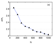
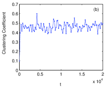
Figure 1: (Color online) (a) The network average path length (APL) decreases as network size increases from 100 to 1000 vertices. (b) The evolution of the clustering coefficient.

As we know, “small-world networks” are characterized by a high degree of clustering and a small average path length which scales logarithmically with the number of vertices [2]. We can see from the above analysis that the network has a large clustering coefficient and a small average path length, and the average path length decreases with the increases of the network size, so the network is a small-world network.

We plot the degree distribution [2] of the resulting network in Fig. 2. The distribution looks like a Poisson distribution, but it is “fatter” on the right hand side of the peak than on the left hand side. In the above rules, the reproduction of offspring can be seen as a kind of preferential attachment in complex network theory (the increase of new interactions is also a kind of preference). But the offspring genome is mainly a copy of the parent’s one: if the parent has good health, the offspring will also have good health (and high activity on becoming mature) with a high probability, and this will increase the number of individuals with high activity, so in the attachment the preferential effect will be decreased and the random effect will be increased. Due to the effect of mutation, the offspring who has a healthy parent will lose good genome with a certain probability, which will also increase the randomness of the attachment. So, the degree distribution should be a result of the combination of preferential attachment (power-law distribution) and random attachment (Poisson distribution). This explains the degree distribution in Fig. 2. It is known that the distribution of many real networks can also be seen as a combination of power-law and Poisson distributions.

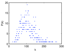
Figure 2: (Color online) The degree distribution

Assortative mixing is also an important property of many networks, especially social networks. A network is said to show assortative mixing if the vertices in the network that have many connections tend to be connected to other vertices with many connections [5, 12]. Assortative mixing can have profound effect on the properties of a network. For example, it is found that assortative networks are more robust to removal of their highest degree vertices than the disassortative ones. To measure the assortative property of a network, we can calculate the assortative coefficient. For mixing by vertex degree in an undirected network, the assortative coefficient is [5, 6]

$$r=\frac{M^{-1}\sum_{i}j_{i}k_{i}-[M^{-1}\sum_{i}\frac{1}{2}(j_{i}+k_{i})]^{2}}{M^{-1}\sum_{i}\frac{1}{2}(j_{i}^{2}+k_{i}^{2})-[M^{-1}\sum_{i}\frac{1}{2}(j_{i}+k_{i})]^{2}},$$ (4)

where $j_{i},k_{i}$ are the degrees of the two vertices at the ends of the $i$th edge, with $i=1,2,\cdots,M$. The coefficient is in the range $-1\leq r\leq 1$, and if $r$ is positive, the network is assortative.

For a network with $N_{max}=500$ created by the above evolution rules [13], we calculate the value of $r$ according to Eq. (4), and obtain that $r=0.4952$, which indicates strong assortative mixing in this network. The scatter plot of the degrees of pairs of vertices at the two ends of links is shown in Fig. 3 (a), and the histogram of the degree differences between pairs of vertices at the two ends of links is shown in Fig. 3 (b). From this figure, we see that the network shows assortative mixing. In fact, in the evolution of the population, there are individuals removed in each time step, so the evolution of the network is robust to the removal of vertices (including highest degree vertices), and has self-repair ability.

Figure 3: (Color online) (a): Scatter plot of the degrees of pairs of vertices at the two ends of links. (b): The histogram of the degree differences between pairs of vertices at the two ends of links.

In summary, in this paper, we studied the evolution of a modified Penna model, and showed that when taking the social interactions into account, the individuals form a complex network. The properties of the network were studied by computer simulation. Numerical results indicate that the network has emergent small-world and assortative mixing properties. The replication rule is responsible for the small world effect, and the Penna model is responsible for other properties, such as limited node number, ageing effect, and the degree distribution, of the network. This paper, to some extent, mimics the evolution and the formation of social interactions in a society and also provides a network model with many properties observed in real networks, such as evolution, ageing, small-world effect and assortative mixing property. We only studied the asexual case of the Penna model in this paper; the sexual case, as well as other properties [14] and theoretical analysis of the generated network, will be the subject of future research.

References

- (1) T.J.P. Penna, J. Stat. Phys. 78, 1629 (1995); S.M. de Oliveira, Physica A 257, 465 (1998); S.M. de Oliveira, P.M.C. de Oliveira, and D. Stauffer, Evolution, Money, War and Computers,Teubner, Stuttgart and Leipzig, 1999.
- (2) S.H. Strogatz, Nature (London)410, 268 (2001); R. Albert and A.L. Barabási, Review of Modern Physics 74, 47 (2002); S.N. Dorogovtsev and J.F.F. Mendes, Adv. in Phys. 51, 1079-1187 (2002); M.E.J. Newman, SIAM Review 45, 167-256 (2003).
- (3) D.J. Watts, S.H. Strogatz, Nature 393, 440 (1998).
- (4) A.L. Barabási and R. Albert, Science 286, 509 (1999).
- (5) M. E. J. Newman, Phys. Rev. Lett. 89, 208701 (2002).
- (6) M. E. J. Newman, Phys. Rev. E 67, 026126 (2003).
- (7) M. Magdon-Maksymowicz, A.Z. Maksymowicz, and K. Kulakowski, Theory in Biosciences 119, 139 (2000).
- (8) A. O. Sousa, S. M. de Oliveira, Eur. Phys. J. B 9, 365 (1999); E. Brigatti, J.S. Sá Martins, I. Roditi, Eur. Phys. J. B 42, 431 (2004).
- (9) S. Cebrat, Physica A 258, 493 (1998); J. S. Sá Martins, S. Cebrat, Theory in Biosciences 119, 156 (2000).
- (10) R.C. Desai, F. James, E. Lui, Theory in Biosciences 118, 97 (1999).
- (11) B. Bollabas, Random Graphs, Academic Press, London, 1985.
- (12) In [6], Newman extended the concept of assortative mixing in networks to “the tendency for vertices in networks to be connected to other vertices that are like them in some way”. In this paper, we only consider mixing by vertex degree, that is, we use, in a narrow sense, the concept of mixing [5].
- (13) For , there are too many points in the scatter plot of Fig. 3, so for the purpose of clarity, we use the results of here.
- (14) L. da F. Costa, F. A. Rodrigues, G. Travieso, and P. R. Villas Boas, cond-mat/0505185.