Power spectrum for critical statistics:
A novel spectral characterization of the Anderson transition

Abstract

We examine the power spectrum of the energy level fluctuations of a family of critical power-law random banded matrices with properties similar to those of a disordered conductor at the Anderson transition. It is shown both analytically and numerically that the Anderson transition is characterized by a power spectrum which presents $1/f^{2}$ noise for small frequencies but $1/f$ noise for larger frequencies. For weak diagonal disorder the analysis of the transition region between these two power-law limits provides with an accurate estimation of the Thouless energy of the system. As disorder increases the Thouless energy looses its meaning and the power spectrum presents a $1/f^{2}$ decay up to frequencies related to the Heisenberg time of the system. Finally we discuss under what circumstances these findings may be relevant in the context of non-random Hamiltonians.

I Introduction

Level statistics is a powerful tool to investigate the properties of quantum complex systems. The spectrum is basis independent and typically easier to access either numerically or experimentally than the eigenfunctions. The analysis of the level statistics is usually carried out in two steps. First the spectrum is properly unfolded, namely, by extracting the mean level density, the original spectrum is transformed into one with a mean level density equal to the unity. In a second stage the unfolded spectrum is analyzed by evaluating different spectral correlators. Two popular choices are the level spacing distribution $P(s)$ (the probability of having two eigenvalues at a distance $s$) for short range correlations and the number variance $\Sigma^{2}(L)=\langle L^{2}\rangle-{\langle L\rangle}^{2}$ (which measures the deviations of the number of eigenvalues in an interval $L$ from its mean value) for long range correlations. In certain situations these spectral correlators present striking universal features. For instance, in the context of deterministic Hamiltonians the celebrated Bohigas-Giannoni-Schmit conjecture oriol states the level statistics of a deterministic quantum system whose classical counterpart is fully chaotic depends not on the microscopic details of the Hamiltonians but only on the global symmetries of the system and are identical to those of a random matrix with the same symmetry, usually referred to as Wigner-Dyson statistics (WD) mehta .

Remarkably the same WD statistics also describes efetov the spectral correlations of a disordered system in the metallic limit. In the strong disorder limit localization sets in, the spectrum is not correlated and the level statistics is universally described by Poisson statistics. For deterministic systems the same statistics is generic of systems whose classical dynamics is integrable tabor . From a practical point of view, universality is usually tested by comparing correlators like $P(s)$ or $\Sigma^{2}(L)$ of a specific system with the universal predictions of WD or Poisson statistics.

Recently a different spectral characterization based on techniques of time series was introduced in the context of quantum chaos rel ; rel1 . In rel ; rel1 the unfolded energy spectrum is formally considered as a discrete signal and the energy levels are interpreted as a time series. Specifically they investigate the power spectrum,

$$S(k)=\left|{1\over\sqrt{N}}\sum_{n=1}^{N}\delta_{n}\exp{\left({-2\pi ikn\over N}\right)}\right|^{2}\;,$$ (1)

of the sequence $\delta_{n}$

$$\delta_{n}=\sum_{i=1}^{n}\left(s_{i}-{\bar{s}}\right)=\epsilon_{n+1}-\epsilon_{1}-n,$$ (2)

where $s_{i}=\epsilon_{i+1}-\epsilon_{i}$, $\epsilon_{i}$ is ith unfolded eigenvalue and $N$ is the length of the series. The correlator $\delta_{n}$ thus gives the deviation of the ith nearest neighbor spacing $s_{i}$ from its mean value ${\bar{s}}$ which by definition is the unity for unfolded eigenvalues.

It was found that the $S(k)$ for systems whose classical counterpart is completely chaotic or integrable has a universal power-law form with an exponent depending on the classical dynamics: $S(k)\sim 1/k$ for chaotic and $S(k)\sim 1/k^{2}$ for integrable motion.

Universality in the spectral correlations has also a counterpart in the eigenfunctions properties. Thus Poisson statistics is associated with exponential localization of the eigenfunctions and WD statistics is typical of systems in which the eigenstates are delocalized through the sample and can be effectively represented by a superposition of plane waves with random phases.

Despite its robustness, these universal features are restricted to long time scales (related to energy scales of the order of the mean level spacing) such that an initially localized wave-packet has already explored the whole phase space available. In other words, universality is related to certain ergodic limit of the quantum dynamics. For shorter time scales the system has not yet relaxed to the ergodic limit and deviations from universality are expected. For finite disordered systems this scale is given by the dimensionless conductance $g=E_{c}/\Delta$ ($E_{c}$, the Thouless energy, is a scale of energy associated with the classical diffusion time through sample and $\Delta$ is the mean level spacing) which roughly speaking gives the number of eigenvalues whose spectral correlations are universally described by WD statistics.

Striking universal features not related to any ergodic limit (they persist beyond the mean level spacing scale) have also been observed in a disordered system at the metal-insulator transition also referred to as Anderson transition (AT). It is by now well established that a disordered system with short range hopping in more than two dimensions undergoes an AT anderson ; wegner at the center of the band for a critical amount of disorder (for critical we mean a disorder such that if increased all the states in the band become exponentially localized). Since the dimensionless conductance $g\sim 1$ is about the unity at the 3D (or 4D) AT, the level statistics for eigenvalues separations larger than the mean level spacing describes truly dynamical features of the system. By universality we mean that the level statistics do not depend on boundary conditions, shape of the system or the microscopic details of the disordered potential though some features may depend on the dimensionality of the space.

Signatures of the AT are found in both the level statistics and the eigenfunctions. Systems belonging to this new universality class have multifractal eigenstates. Intuitively multifractality means that the eigenstates have structures at all scales. In a more formal way multifractality is defined through the anomalous scaling of the eigenfunctions moments ${\cal P}_{q}=\int d^{d}r|\psi({\bf r})|^{2q}$ with respect to the sample size $L$ as ${\cal P}_{q}\propto L^{-D_{q}(q-1)}$, where $D_{q}$ is a set of different exponents describing the AT aoki .

Level statistics at the AT (commonly referred to as ’critical statistics kravtsov97 ) is intermediate between WD and Poisson statistics. Although a formal definition is still missing, typical features of critical statistics include: scale invariant spectrum sko , level repulsion and linear number variance ($\Sigma_{2}(L)\sim\chi L$) chi as for a insulator ($\chi=1$) but with a slope $\chi<1$ ($0.27$ for the 3D Anderson transition). Similar spectral properties has also been found in random matrix models based on soft confining potentials log , effective eigenvalue distributions Moshe ; ant4 related to the Calogero-Sutherland model calo at finite temperature and random banded matrices with power-law decay evers . The latter is specially interesting since an AT (for the case $1/r$ decay) has been analytically established by mapping the problem onto a non linear $\sigma$ model.

In this paper we propose an alternative spectral characterization of the Anderson transition based on the analysis of the power spectrum $S(k)$ introduced above. We shall also see this technique provides with an accurate way to locate the Thouless energy of a disordered system. Finally we will discuss the relevance of our findings in the context of non random system. It will shown that $S(k)\sim 1/k^{2}$ is not always related to integrable classical motion. Consequently a precise classificatory scheme based on $S(k)$ must have into account other features of $S(k)$ besides the exponent of the power-law decay.

The organization of the paper is as follows. In the next section the model to be investigated is introduced. The power spectrum $S(k)$ is evaluated both analytically and numerically for a broad range of parameters in section three and four. From these results we present a novel spectral characterization of the Anderson transition based on the analysis of $S(k)$. We will also argue that this technique can be utilized to detect the Thouless energy in a disordered system. Finally in section five we discuss in what situations our findings may be relevant for non-random quantum systems.

II The model

In this section we evaluated both analytically and numerically the power spectrum $S(k)$ of a critical random banded matrix associated to critical statistics.

Unlike WD or Poisson statistics, critical statistics is not parameter free. Together with universal features such as scale invariance, level repulsion and linear number variance $\Sigma^{2}(L)=\chi L~{}~{}L\gg 1$, there are also system dependent features as the numerical value of the slope of the number variance $\chi$. For instance, for short range Anderson models, this slope depends on the Euclidean dimension $d$ of the sample. Thus for the lower critical dimension $d=2+\epsilon$ ($\epsilon>0$) wegner , $\chi\sim\epsilon\ll 1$. In the opposite limit $d\gg 1$, $\chi\leq 1$ is close to the unity similar to the case of an insulator.

In this letter, instead of studying directly these short range Anderson model, we will focus on certain generalized random matrix models which has been shown to reproduce critical statistics kravtsov97 with great accuracy. An advantage of these models is that exact analytical solutions are available in a certain region of parameters Moshe ; evers ; log .

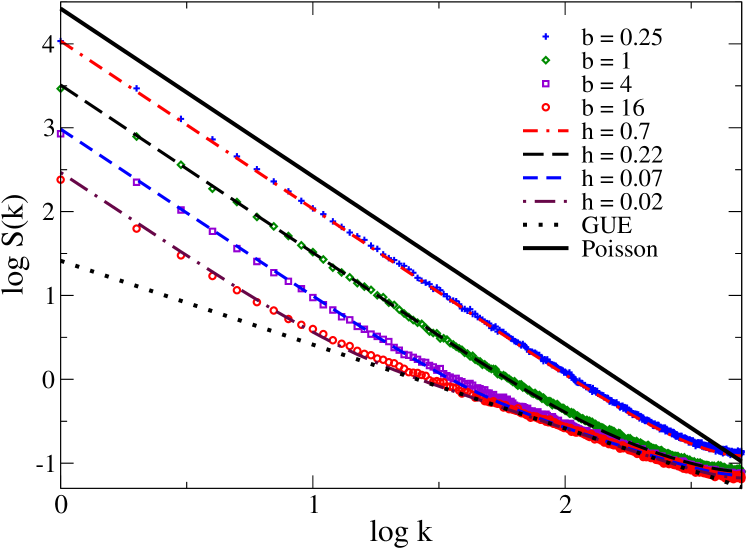
Figure 1: Power spectrum $S(k)$ as a function of $k$. Symbols represent the numerical results (the matrix size is $3000$ and the number of eigenvalues considered is $N=1024$ around the center of the band) for the critical random banded model Eq.3 for different bandwidth $b$, the power spectrum was evaluated from Eq. 7. Lines represent the analytical prediction of critical statistics Eq. 11 with the TLCF given by Eq. 6. For all $b$ the agreement between theory and numerics is excellent. As predicted for $b\gg 1$ we observe two different regions: $N/k\gg 2\pi b$ corresponding with $S(k)\sim 1/k^{2}$ and $N/k\ll 2\pi b$ with $S(k)\sim 1/k$ similar to the prediction of WD (GUE). However for $b\ll 1$, $S(k)\sim 1/k^{2}$ for almost all $k$.

We investigate the ensemble of random complex Hermitian matrices $\hat{H}$. The matrix elements $H_{ij}$ are independently distributed Gaussian variables with zero mean $\langle H_{ij}\rangle=0$ and variance

$$\langle|H_{ij}|^{2}\rangle=\\ \left[1+{1\over b^{2}}{\sin^{2}(\pi(i-j)/N)\over(\pi/N)^{2}}\right]^{-1}\ ,$$ (3)

For any value of the bandwidth $0<b<\infty$, the spectral correlations are given by critical statistics and the eigenvectors are multifractal exactly as at the conventional Anderson transition in $2<d<\infty$ evers . The limit $b\rightarrow\infty$ corresponds with the standard Gaussian Unitary Ensemble (GUE) of random matrices. The region $b\gg 1$ (weak diagonal disorder, $\chi\ll 1$) corresponds with $d=2+\epsilon$ ($\epsilon\ll 1$) and the $b\ll 1$ limit with $d\gg 1$ and $\chi\leq 1$ (strong diagonal disorder). For Hermitian matrices these two limits are accessible to analytical techniquesevers ; kra2005 . Here we do not discuss the details of these calculations but just enumerate certain results we will use later on in the calculation of the power spectrum $S(k)$.

For $b\gg 1$ the level statistics can be rigorously investigated after mapping the random banded matrix onto a supersymmetry sigma model. It can be shown evers that in this limit the connected part of two level correlation function (TLCF) is given by,

$$R_{2}(s)=\frac{\langle\rho(s/2)\rho(-s/2)\rangle}{\langle\rho(0)\rangle^{2}}-1=\delta(s)-\frac{1}{16b^{2}}\frac{\sin^{2}(\pi s)}{\sinh^{2}(\pi s/4b)}$$ (4)

where $\rho(s=E/\Delta)=\sum_{i}\delta(s_{i}-s)$ is the spectral density in units of the mean level spacing $\Delta=1/\langle\rho(0)\rangle$ and brackets stand for ensemble average.

For $b\ll 1$, various spectral correlators can also by calculated explicitly by a recently developed virial expansion around the Poisson limit kra2005 (for a more heuristic approach see evers ).

The intermediate region of $b\sim 1$ is not yet accessible to analytical techniques. However there is a closely related random matrix model Moshe which is exactly solvable for any $b$ and which has the same TLCF (to leading order in $b$) in the two regions ($b\ll 1,b\gg 1$) above discussed. Its joint probability distribution is given by

$$P(H,b)=\int dUe^{-\frac{1}{2}{\rm Tr}HH^{{\dagger}}}e^{-\frac{b}{2}{\rm Tr}{[U,H][U,H]^{{\dagger}}}}.$$ (5)

Here, the $N\times N$ matrices $H$ and $U$ are Hermitian and Unitary, respectively, and the integration measure $dU$ is the Haar measure. Despite its complicated form, it can be shown Moshe ; ant4 that the joint distribution of eigenvalues of $H$ is equal to the diagonal element of the density matrix of a system of free spinless fermions at finite temperature $T=1/b$ confined in an harmonic potential. By using elementary statistical mechanics techniques it can be shown that the TLCF for arbitrary $b$ is given by,

$${R_{2}}(s)=\delta(s)-\left(\int_{0}^{\infty}\frac{\cos(\pi st/\rho(0))}{\rho(0)}\frac{1}{{1+ze^{t^{2}}}}dt\right)^{2}$$ (6)

where $h=1/2\pi b$,$z=\frac{1}{e^{1/h}-1}$ and $\rho(0)=\int_{0}^{\infty}\frac{1}{1+ze^{t^{2}}}$. We shall use this expression in the analytical evaluation of the power spectrum for intermediate values of $b$ and then check its validity by carrying out numerical simulations of the random banded model Eq. 3.

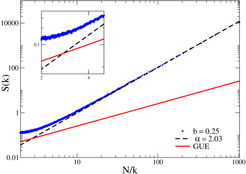
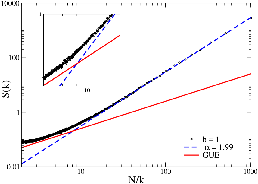
Figure 2: Power spectrum $S(k)$ versus $N/k$ in the limit $b\leq 1$. Crosses and circles represent the numerical results (the matrix size is $3000$ and the number of eigenvalues considered is $N=1024$ around the center of the band) for the critical random banded model Eq. 3 for $b=0.25,1$ respectively. The power spectrum was evaluated from Eq. 7. The dashed line corresponds to the best fit $S(k)=1/k^{\alpha}$ (the error in $\alpha$ is about $\Delta\alpha=\pm 0.02$) in the limit $N/k\gg 2\pi b$ and the solid line is the prediction of WD statistics obtained from the GUE. The intersection between the linear fit and the WD statistics prediction corresponds in principle with the Thouless energy of the system. However we observe that, for $b\leq 1$, $S(k)$ is always different from the WD prediction and consequently no clear Thouless energy can be defined.

III Analytical evaluation of $S(k)$. Power spectrum characterization of critical statistics.

Our goal is to compute the power spectrum

$$\langle S(k)\rangle=\left\langle\left|{1\over\sqrt{N}}\sum_{n=1}^{N}\delta_{n}\exp{\left({-2\pi ikn\over N}\right)}\right|^{2}\right\rangle\;,$$ (7)

with $\delta_{n}=\sum_{i=1}^{n}s_{i}-{\bar{s}}=\epsilon_{n+1}-\epsilon_{1}-n$, $\epsilon_{n}$ represents the nth unfolded eigenvalue of the critical random banded model Eq. (3) and the brackets stand for ensemble average.

In a first stage we evaluate $\langle S(k)\rangle$ in a continuous approximation, $\langle S(k)\rangle=\langle S(k)\rangle_{cont}$, $\sum\rightarrow\int$, $s_{i}\rightarrow\rho(\epsilon)d\epsilon$ and ${\bar{s}}\rightarrow{\bar{\rho}(\epsilon^{\prime})}d\epsilon^{\prime}$ where $\rho(\epsilon)=\sum_{i}\delta(\epsilon-\epsilon_{i})$ is the full spectral density and ${\bar{\rho}(\epsilon)}$ is just the smooth part of it (the one utilized to unfold the spectrum).

The power spectrum is now given by,

$$\langle S(k)\rangle_{cont}=\left\langle\left|\int d\epsilon\delta^{\prime}(\epsilon)\exp{\left({-2\pi\epsilon k}\right)}\right|^{2}\right\rangle=\left\langle\int_{-\infty}^{+\infty}\int_{-\infty}^{+\infty}d\epsilon^{\prime}d\epsilon\exp(-2\pi i(\epsilon-\epsilon^{\prime})k)\int^{\epsilon^{\prime}}\int^{\epsilon}{\tilde{\rho}}(\alpha){\tilde{\rho}}(\alpha^{\prime})d\alpha^{\prime}d\alpha\right\rangle$$ (8)

with $\delta^{\prime}(\epsilon)=\int^{\epsilon}d\epsilon{\tilde{\rho}}(\epsilon)$ and ${\tilde{\rho}}(\epsilon)=\rho(\epsilon)-{\bar{\rho}}(\epsilon)$.

After integrating by parts in $\epsilon$ and $\epsilon^{\prime}$ the above expression simplifies to,

$$\langle S(k)\rangle_{cont}=\frac{1}{4\pi^{2}k^{2}}\int_{-\infty}^{+\infty}\int_{-\infty}^{+\infty}d\epsilon^{\prime}d\epsilon\exp(-2\pi i(\epsilon-\epsilon^{\prime})k)R_{2}(\epsilon,\epsilon^{\prime})$$ (9)

where $R_{2}(\epsilon,\epsilon^{\prime})$ is the TLCF defined previously. Since the spectrum is translational invariant (if we are far from the edges) $R_{2}(\epsilon,\epsilon^{\prime})=R_{2}(s=\epsilon-\epsilon^{\prime})$ and

$$\langle S(k)\rangle_{cont}=\frac{1}{4\pi^{2}k^{2}}\int_{-\infty}^{\infty}\exp(-2\pi isk)R_{2}(s)=\frac{1}{4\pi^{2}k^{2}}K(k)$$ (10)

where $K(k)$, the Fourier transform of the TLCF, is usually referred to as the spectral form factor.

Once we have obtained an explicit expression for the power spectrum in terms of known quantities as $R_{2}(s)$ we have to go back to the original discrete formulation. This can be easily done by following standard relations between the discrete and the continuous Fourier transform, we only present the final result and refer to four ; rel1 for additional details,

$$S(k)=\frac{K(t)}{4\pi^{2}t^{2}}+\sum_{q=1}^{\infty}\frac{K(t+q)}{4\pi^{2}(t+q)^{2}}+\frac{K(q-t)}{4\pi^{2}(q-t)^{2}}+\beta$$ (11)

with $t=k/N$ and $\beta$ a constant given by $\beta=[K(0)-1]^{2}/12$ which accounts for the differences between the fluctuations of $\int^{\epsilon^{\prime}}\int^{\epsilon}\langle{\tilde{\rho}}(\alpha){\tilde{\rho}}(\alpha^{\prime})\rangle d\alpha^{\prime}d\alpha$ and those of the original discrete correlator $\delta_{n}$ (see four for details). For the sake of simplicity we set $\langle S(k)\rangle=S(k)$. The above expression combined with Eq 4,6 provides with a closed and compact expression for the power spectrum as a function of the band size $b=1/2\pi h$.

In the region of $b\gg 1$ the spectral form factor can be explicitly evaluated by using the TLCF of Eq.(4).

$$K(t)=1-\frac{1}{2}\left[(1-t)\coth\left(\frac{2-2t}{h}\right)+(1+t)\coth\left(\frac{2+2t}{h}\right)-2t\coth\left(2t/h\right)\right]$$ (12)

We can distinguish two different regions. For $t\ll h=1/2\pi b$, corresponding to eigenvalues separated a distance much larger than the mean level spacing, $K(t)\sim h/2$ is a constant and $S(k)\sim h/(8\pi^{2}t^{2})$, similar to the case of Poisson statistics. However for Poisson $K(0)=1$ but in our case $K(0)=h/2$. This is an important difference since Poisson statistics is associated with eigenstates exponentially localized but for $K(0)=\chi\neq 1$ (where $\chi$ is the slope of the number variance) the eigenstates are multifractal.

It seems that, at least in this case, the exponent of the decay of $S(k)$ does not completely specify the nature of the quantum motion. We will go back to this point when we discuss applications of our work in the context of quantum chaos.
In the opposite limit $t\gg h=1/2\pi b$, $K(t)=t$ and $S(t)\sim 1/(2\pi^{2}t)$ in agreement with the result for WD statistics (GUE).

The transition region separating the two types of decay ($1/t$ and $1/t^{2}$) corresponds to the Thouless energy of the system. As usual it separates short range correlations still controlled by WD statistics from larger scales in which typical features of the AT appear.

We have thus found that the power spectrum in the limit $b\gg 1$ corresponding to the case of a disordered system in $2+\epsilon$ dimensions with short range disorder at the AT has different power-law decay depending of the spectral region of interest, these differences can be effectively utilized to find signatures of an AT from a given spectrum.

Analogously, in the region $b=1/2\pi h\ll 1$, which corresponds with the case of disordered conductor in $d\gg 1$, a straightforward calculation shows that $K(t)=1-1/\sqrt{2}h$ for $t\ll h$ and then goes to $K(t)=1$ for $t\gg h$. Consequently $S(t)\sim 1/t^{2}$ up to scales smaller than the mean level spacing. Strictly speaking there is a narrow transition region already for $t>1$ in which $K(t)$ is linear However it is difficult to interpret it as a Thouless energy since even for scales shorter than the mean level spacing the spectral correlations are different from WD statistics.

Finally we mention that for intermediate $b$ there is not a rigorous analytical relation for the TLCF. However we shall see that the conjecture Eq (6) describes very accurately the numerical results (see Fig 1).

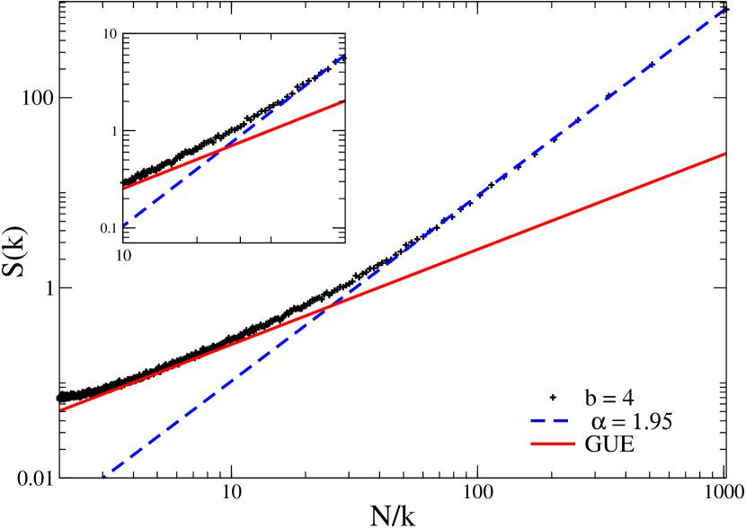
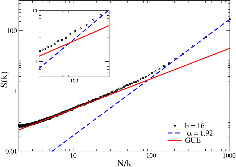
Figure 3: Power spectrum $S(k)$ versus $N/k$ in the limit $b\gg 1$. Crosses and circles represent the numerical results (the matrix size is $3000$ and the number of eigenvalues considered is $N=1024$ around the center of the band) for the critical random banded model Eq.3 for $b=4,16$ respectively. The power spectrum was evaluated from Eq. 7. The dashed line corresponds to the best fit $S(k)=1/k^{\alpha}$ (the error in $\alpha$ is about $\Delta\alpha=\pm 0.02$) in the limit $N/k\gg 2\pi b$ and the solid line is the prediction of WD statistics obtained from the GUE. The intersection between the linear fit and the WD prediction corresponds with the Thouless energy of the system. The units has been chosen such that the intersection point gives the dimensionless conductance of the system $g$. Thus $g\sim 25$ for $b=4$ and $g\sim 100$ for $b=16$.

IV Numerical calculations

We now investigate numerically the random banded model in Eq.3 in order to test the analytical predictions of the previous section.

We studied the power spectrum $S(k)$ by direct diagonalization of the critical random banded matrix Eq.3 for different matrix sizes (almost all of our plots are for $3000$ though we try higher volumes, up to $5000$, in order to check that our results are not size dependent). The number of different realizations of disorder is chosen such that for each matrix size the total number of eigenvalues be at least $2\times 10^{6}$. Typically around $35\%$ of the eigenvalues around the center of the band are utilized. The eigenvalues thus obtained are unfolded with respect to the mean spectral density. The power spectrum is calculated by using Eq.7 where the Fourier transform is evaluated by using a fast Fourier transformation routine.

In Fig 1 we have plotted $\log S(k)$ for different $b$. In all cases the matrix size was $3000$ and the evaluation of $S(k)$ was carried out within a band around the center of the spectrum containing $1024$ eigenvalues. As observed the agreement between the analytical (with $R_{2}(s)$ given by Eq.(6) and $h=1/2\pi b$) and numerical results is excellent for all $b$. Also in agreement with the analytical prediction we observe that, for $b\gg 1$, the power spectrum switches from $S(k)\sim 1/k$ for $N/K\ll h=1/2\pi b$ to $S(k)\sim 1/k^{2}$ in the opposite limit. However for $b\ll 1$, $S(k)\sim 1/k^{2}$ for almost all accessible frequencies.
We conclude after the analytical and numerical analysis that the AT in a disordered conductor can be satisfactorily detected and examined by looking at the power spectrum of a signal $\delta_{n}$ consisting of the fluctuations around its mean value of the nearest neighboring spacings $s_{i}=\epsilon_{i+1}-\epsilon_{i}$.

We have also found that $S(k)$ provides with an accurate method to locate the Thouless energy of a generic disordered conductor. As mentioned previously, the Thouless energy $E_{c}$ is a scale of energy related with the classical diffusion time through the sample. In units of the mean level spacing $\Delta$ it gives the dimensionless conductance $g$, namely, the number of eigenvalues $g=E_{c}/\Delta$ for which the universal results of WD statistics apply. From a practical point of view the evaluation of $g$ from a given spectrum is a hard task since it may depend on what spectral correlator is used. Thus $\Sigma^{2}(L)$ gives a prediction of $g$ bigger than that of $P(s)$ but much smaller than that of the spectral rigidity $\Delta_{3}(L)$ (see mehta for a definition). Another problem is that even for each particular correlator the value of $g$ is somewhat ambiguous since it is far from clear how to locate even approximately the point in which WD ceases to be applicable.
Below we show that $S(k)$ provides with a more efficient and precise way to locate and analyze $g$. The idea (see Fig 2 and Fig 3) is to plot $S(k)$ as a function of $N/k$. Then in the region $N/k\gg 2\pi b$ we fit $S(k)$ to a linear (in a log scale) curve $S(k)\sim 1/k^{\alpha}$ (from the previous analysis $\alpha\sim 2$). In the opposite limit $S(k)$ should be given by the prediction of WD statistics. We define the Thouless energy as the intersection between the WD prediction and the linear fit.

In Fig 2 we see that for $b\gg 1$ the intersection of these two curves gives $g\sim 2\pi b\gg 1$ in good agreement with the theoretical prediction. However in the region $b\leq 1$ (see Fig 3), though formally a Thouless energy can be defined thorough the intersection of the two curves, its interpretation as the limit of applicability of WD statistics is dubious since even in the limit $N/k\ll 2\pi b$ deviations with respect to the WD prediction are clearly visible.

Finally we mention that, as observed in Fig 1, the best fit of the numerical results does not occur at the analytical estimation $h=1/2\pi b$. There are two reasons for that disagreement: The analytical results are strictly valid only at the center of the band. Eigenstates beyond this region are still critical but are described by an effective bandwidth cambridge smaller than $b$. On the other hand finite size effects are important in the limit $t\rightarrow 0$ since we are testing the largest eigenvalue separations. However we have decided not to reduce the spectral window in order to give a full global picture of the power spectrum at the AT. After all, as shown in Fig 1, these effects are easily compensated by slightly modifying $b$.

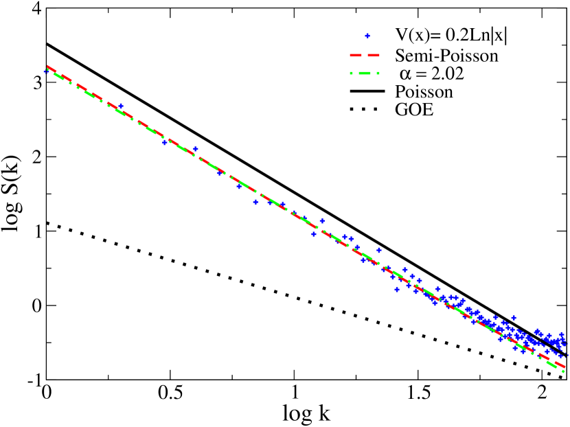
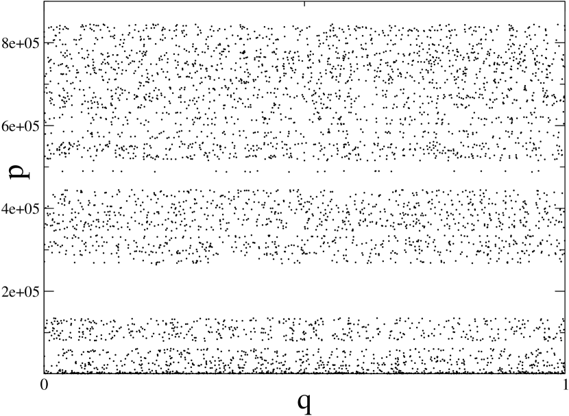
Figure 4: (Left) Power spectrum $S(k)$ obtained from $25$ set of $256$ eigenvalues after the numerical diagonalization of the evolution matrix associated to Eq. (13) with $V(q)=0.2Ln|q|$ (cross). The dashed line is the prediction of SP statistics, the dotted-dashed line is the best fit $S(k)\sim 1/k^{\alpha}$ and the dotted line is the prediction of WD statistics as obtained from the Gaussian Orthogonal Ensemble (GOE) of random matrices. (Right) Poincare section from a single initial condition $p_{0}=0.2$ and $q_{0}=0.6$ after 300000 iterations.

V Application to quantum chaos

In this final section we investigate possible applications of our previous findings in the context of quantum chaos and also argue that $S(k)\sim 1/k^{2}$ is not exclusive of quantum deterministic system whose classical counterpart is integrable.

Critical statistics and multifractal wavefunctions are very much universal so they should also appear in deterministic quantum systems. Indeed, in a recent letter ant9 we have established a novel relation between the presence of anomalous diffusion in the classical dynamics, the singularities of a classically chaotic potential and the power-law localization of the quantum eigenstates. Specifically, it was found that for a kicked rotor with Hamiltonian

$${\cal H}=\frac{p^{2}}{2}+V(q)\sum_{n}\delta(t-nT)$$ (13)

(with $q\in[-1,1)$) both level statistics and eigenfunctions are similar to the ones at the AT (critical statistics) provided that $V(q)$ has a $\log$ (in the simplest case $V(q)=\epsilon_{0}Ln|x|$) or a step-like ant11 singularity. It was also found in ant9 that these findings are universal in the sense that neither the classical nor the quantum properties depend on the details of the potential but only on the type of singularity. Deviations from WD statistics not coming from a mixed phase space has also been reported in a variety of systems: Coulomb billiardaltshu , Anisotropic Kepler problem wintgen , a kicked rotor in a well potential bao and pseudointegrable billiards bogo3 ; bogo04 . For the latter it was found bogo3 that the level statistics is accurately described by a the classical Dyson gas with the logarithmic pairwise interaction restricted to a finite number $k$ of nearest neighbors. Analytical solutions are available for general $k$. For $k=2$, usually referred to as semi Poisson (SP) statistics, $R_{2}(s)=1-e^{-4s}$, $P(s)=4se^{-2s}$ and $\Sigma^{2}(L)=L/2+(1-e^{-4L})/8$. We have also found ant11 that SP statistics describes accurately the spectral correlations of the above kicked rotor with a step like singularity and also provides with a reasonable description for the $\log$ singularity but only for $\epsilon_{0}\sim 0.2$.

Due to the simplicity of the TLCF in SP statistics one can evaluate the power spectrum exactly,

$$S(k)=\frac{1}{4\pi^{2}t^{2}}\left[1-\frac{8}{16+4\pi^{2}t^{2}}\right]$$ (14)

Thus the power spectrum associated to SP statistics has $1/t^{2}$ decay even though the classical dynamics is not integrable, this is also in agreement with the prediction of critical statistics for $b\ll 1$. Thus $S(k)\sim 1/t^{2}$ ($t=k/N$) is not always a signature of classical integrable dynamics. Although generically the power spectrum associated with classically integrable systems has this feature, other types of non integrable dynamics may have $1/t^{2}$ as well. In order to fully characterize the classical dynamics from $S(k)$ one has to specify not only the exponent but also and additional point of the curve, for instance $K(0)$. The point is that a $1/t^{2}$ decay only tell us that the form factor is constant. However, as mentioned previously, the physical properties of the system are strongly modified by a spectral form factor different from the unity.

As a further corroboration of our claims we have evaluated numerically $S(k)$ for the Hamiltonian of Eq. 13 with a potential $V(x)=0.2Ln|x|$. We diagonalize numerically the evolution matrix associated to the Hamiltonian Eq.13 for $N=5200$, $S(k)$ is obtained from Eq.7. In order to improve statistics we divide the original spectrum in 20 set of 256 eigenvalues. As shown in Fig 4, $S(k)\sim 1/t^{2}$ for almost all $t$ in close agreement with the prediction of SP or critical statistics. However (see right plot) the associated Poincare section obtained from just a single initial condition is very different from that of an system whose classical dynamics is integrable.

VI Conclusions

We have shown that the power spectrum of the energy level fluctuations at the Anderson transition for a family of critical power-law random banded matrices is characterized by a power spectrum which $1/f^{2}$ noise for small frequencies and $1/f$ noise for larger frequencies. In the weak disorder limit $b\gg 1$, the analysis of the transition region between these two power-law limits provides with an accurate estimation of the Thouless energy of the system. As disorder increases the Thouless energy looses its meaning and the power spectrum presents a $1/f^{2}$ noise up to frequencies related to the Heisenberg time of the system. Finally we discuss under what circumstances these findings may be relevant in the context of non-random Hamiltonians. Specifically it is shown that the exponent of the power-law decay of $S(k)$ does not fully specify the type of motion of the classical counterpart.

We acknowledge financial support from a postdoctoral fellowship of Spanish Ministry of Science and Education.

References

- (1) O. Bohigas, M.J. Gianonni and C. Schmit, Phys. Rev. Lett. 52, 1 (1984).
- (2) M.L. Mehta, ’Random Matrices’, 2nd Ed., Academic Press (San Diego, 1991).
- (3) K.B. Efetov, Adv. Phys. 32 53 (1983).
- (4) M.V. Berry and M. Tabor, Proc. R. Soc. London A 356, 375 (1977).
- (5) A. Relaño, J.M.G. Gómez, R.A. Molina, J. Retamosa, and E. Faleiro, Phys. Rev. Lett. 89, 244102 (2002).
- (6) E. Faleiro, J.M.G. Gómez, R.A. Molina, L. Muñoz, A. Relaño, and J. Retamosa, Phys. Rev. Lett. 93 244101 (2004).
- (7) P.W. Anderson, Phys. Rev. 109, 1492 (1958).
- (8) F. Wegner, Z. Phys. B 36, 209 (1980).
- (9) H. Aoki, J. Phys. 16C, L205 (1983).
- (10) V.E. Kravtsov and K.A. Muttalib, Phys. Rev. Lett. 79, 1913 (1997); K. A. Muttalib, S. Nishigaki, Phys. Rev. E 59, (1999) 2853.
- (11) B.I. Shklovskii, B. Shapiro, B.R. Sears,P. Lambrianides and H.B. Shore, Phys. Rev. B 47, (1993) 11487.
- (12) B.L. Altshuler, I.K. Zharekeshev, S.A. Kotochigova and B.I. Shklovskii, JETP 67 (1988) 62.
- (13) Y. Chen, M. E. H. Ismail, and V. N. Nicopoulos Phys. Rev. Lett. 71, 471 (1993); Y. Chen and K. A. Muttalib, J. Phys.: Condens. Matter 6 L293 (1994).
- (14) A. M. Garcia-Garcia and J.J.M. Verbaarschot, Phys. Rev. E 67, 046104 (2003);V.E. Kravtsov and A.M. Tsvelik, Phys. Rev. B 62, (2000) 9888.
- (15) M. Moshe, H. Neuberger and B. Shapiro, Phys. Rev. Lett. 73, (1994) 1497.
- (16) F. Calogero, J. Math. Phys. 10 2191 (1969); F . Calogero, J. Math. Phys. 10 2197 (1969); F. Calogero, J. Math. Phys. 12 419 (1971).
- (17) A.D. Mirlin, Y.V. Fyodorov, F.-M. Dittes, J. Quezada, and T.H. Seligman, Phys. Rev. E 54 3221 (1996); E. Cuevas, et.al., Phys. Rev. Lett. 88 016401 (2002);F. Evers and A.D. Mirlin, Phys. Rev. Lett. 84, 3690 (2000);I. Varga, Phys. Rev. B 66, 094201 (2002),E. Cuevas, Phys. Rev. B 68, 184206 (2003).
- (18) O. Yevtushenko and V. Kravtsov, J.Phys. A36 (2003) 8265; V.E. Kravtsov, O. Yevtushenko, E. Cuevas,cond-mat/0510378.
- (19) C. J. Paley, S. N. Taraskin and S. R. Elliott, Phys. Rev. B 72 033105 (2005).
- (20) J.B. French, P. A. Mello, A. Pandey Ann. Phys. (N.Y.) 113 277 (1978); O. Bohigas, P. Leboeuf, M.-J. Sanchez, Found. Phys. 31 (2001) 489.
- (21) A.M. Garcia-Garcia, J. Wang, Phys. Rev. Lett. 94, 244102 (2005).
- (22) A.M. Garcia-Garcia, cond-mat/0507272.
- (23) B.L. Altshuler, L. S. Levitov, Phys. Rep. 288, 487 (1997).
- (24) D. Wintgen and H. Marxer, Phy. Rev. Lett. 60, 971 (1988).
- (25) B. Hu, B. Li, J. Liu and Y. Gu, Phys. Rev. Lett. 82 (1999) 4224; J. Liu, W. T. Cheng, C.G. Cheng, Comm. Theor. Phys. 33 15 (2000).
- (26) E. B. Bogomolny, U. Gerland and C. Schmit, Phys. Rev. E, 59 (1999) R1315.
- (27) E.B. Bogomolny, C. Schmit, Phys. Rev. Lett. 92, 028944, (2004).