Molecular Dynamics Study
of Orientational Cooperativity in Water

Abstract

Recent experiments on liquid water show collective dipole orientation fluctuations dramatically slower then expected (with relaxation time $>$ 50 ns) [D. P. Shelton, Phys. Rev. B 72, 020201(R) (2005)]. Molecular dynamics simulations of SPC/E water show large vortex-like structure of dipole field at ambient conditions surviving over 300 ps [J. Higo at al. PNAS, 98 5961 (2001)]. Both results disagree with previous results on water dipoles in similar conditions, for which autocorrelation times are a few ps. Motivated by these recent results, we study the water dipole reorientation using molecular dynamics simulations in bulk SPC/E water for temperatures ranging from ambient 300 K down to the deep supercooled region of the phase diagram at 210 K. First, we calculate the dipole autocorrelation function and find that our simulations are well-described by a stretched exponential decay, from which we calculate the orientational autocorrelation time $\tau_{a}$. Second, we define a second characteristic time, namely the time required for the randomization of molecular dipole orientation, the self-dipole randomization time $\tau_{r}$, which is an upper limit on $\tau_{a}$; we find that $\tau_{r}\approx 5\tau_{a}$. Third, to check if there are correlated domains of dipoles in water which have large relaxation times compared to the individual dipoles, we calculate the randomization time $\tau_{\rm box}$ of the site-dipole field, the net dipole moment formed by a set of molecules belonging to a box of edge $L_{\rm box}$. We find that the site-dipole randomization time $\tau_{\rm box}\approx 2.5\tau_{a}$ for $L_{\rm box}\approx 3$Å, i.e. it is shorter than the same quantity calculated for the self-dipole. Finally, we find that the orientational correlation length is short even at low $T$.

I Introduction

Cooperative motion of water molecules review has been widely investigated in recent years, both by experiments experiment ; experiment2 ; experiment3 ; experiment4 ; experiment5 ; experiment6 ; experiment7 ; experiment8 ; experiment9 ; experiment10 ; experiment11 ; experiment12 ; experiment13 ; experiment14 ; experiment15 ; experiment16 ; xie93 ; r148 ; dec-models ; shelton and using molecular dynamics (MD) simulations MD ; MDb ; MD2 ; MD2b ; netz ; models ; coupling ; fabbian ; confined-coupling ; models-rot ; semischematicMCT ; MMCT ; trans-rot-coupl ; masaki . When water is cooled, the cooperativity of water molecules increases. Recent experiments on water show large correlated domains of dipoles at ambient conditions which have a relaxation time much larger than the autocorrelation time of individual dipoles shelton . MD studies of water models also show the possibility of formation of large correlated domains of dipoles in bulk as well as interfacial water masaki (where these correlated patterns of dipoles are pinned to solvated amino acids). These two studies are the principal motivation for the present investigation of the rotational cooperativity of water molecules.

A challenging problem is to develop methods of describing molecular motion in water that are better able to interpret experimental results, such as incoherent quasielastic neutron scattering, light scattering, dielectric, and nuclear magnetic resonance experiments experiment ; xie93 . Several approximation proposals have been made for various autocorrelation functions describing both rotational and translational motion dec-models ; models . These methods usually assume the Kohlrausch-Williams-Watts stretched exponential for the long time relaxation behavior of autocorrelation functions $\phi(t)$, as predicted by mode coupling theory (MCT),

$$\phi(t)=A\exp\left[-\left(\frac{t}{\tau_{a}}\right)^{\beta}\right].$$ (1)

The relaxation time $\tau_{a}$, the exponent $\beta$, and the non-ergodicity factor $A$ are fitting parameters that depend on temperature $T$ and density $\rho$ MD ; MDb ; MD2 ; MD2b ; models ; coupling ; fabbian ; confined-coupling ; models-rot .

Our interest here is to study the orientational dynamics of water by simulating SPC/E water. First we calculate the orientational autocorrelation time as the fitting parameter $\tau_{a}$ appearing in Eq. (1) MD ; MDb . Other definitions are possible, e.g., based on other fitting functions for the orientational autocorrelation function decay, such as the biexponential netz ; yeh or the von Schweidler law MMCT . In all cases, the orientational autocorrelation times are the result of multi-parameter fitting procedures and roughly correspond to the characteristic time over which the orientational autocorrelation function decays by a factor of $e\approx 2.7$.

To find an upper limit of the orientational autocorrelation time $\tau_{a}$, we will introduce a new quantity, the dipole randomization time $\tau_{r}$, as the time after which the fluctuations of the dipoles resemble an uncorrelated random variable binder (Sec. IV A). We find $\tau_{r}>\tau_{a}$, and that $\tau_{r}$ and $\tau_{a}$ are linearly related (Sec. IV B), which is consistent with the MCT predictions that:

• The autocorrelation times of all the autocorrelation functions of any fluctuation coupled to density fluctuations diverge at the same temperature $T_{\rm MCT}$ with the same power law exponent;

• All the characteristic times of a supercooled liquid are proportional to one another.

To characterize the increase of cooperativity and test for the presence of large correlated domains of dipoles, we also estimate the randomization time $\tau_{\rm box}$ for the site-dipole field (Sec. V), a quantity which measures the relaxation of the net dipole moment of all the molecules inside a box of edge $L_{\rm box}$. Our calculations show that $\tau_{\rm box}$ when $L_{\rm box}\approx 3$Å has a power law divergence at $T_{\rm MCT}$, but with $\tau_{\rm box}<\tau_{r}$. This result shows that the site-dipole field relaxes faster than the individual dipoles, resolving the apparent contradiction between Ref. masaki and previous results. Calculations of $\tau_{\rm box}$ for larger boxes show that $\tau_{\rm box}$ does not depend on the box size and hence do not support the experimental observation of long-lived large domains of correlated dipoles shelton .

II The SPC/E model

Our results are based on MD simulations of the extended simple point charge (SPC/E) model spce . The distance between the oxygen atom and each of the hydrogen atoms is $0.1$ nm, and the HOH angle is the tetrahedral angle 109.47^∘ realH2O . Each hydrogen atom has a charge $q_{H}=0.432e$, where $e$ is the electron charge, and the oxygen atom has a charge $q_{O}=-2q_{H}$. In addition, to model the van der Waals interaction, pairs of oxygen atoms of different molecules interact with a Lennard-Jones potential,

$$V_{i,j}(r_{i,j})=4\epsilon\left[\left(\frac{\sigma}{r_{i,j}}\right)^{12}-\left(\frac{\sigma}{r_{i,j}}\right)^{6}\right],$$ (2)

where $r_{i,j}$ is the distance between molecules $i$ and $j$, $\epsilon=0.65$ kJ/mol and $\sigma=0.3166$ nm.

We perform MD simulations for a system of $N=1728$ molecules at density $\rho=1.0$ g/cm³, 210 K $\leq T\leq$ 300 K, with periodic boundary conditions and a simulation time step of 1 fs. The temperature is controlled by the Berendsen method of rescaling the velocities berendsen . The long-range Coulombic interactions reactionfield are treated with the reaction field technique with a cutoff of $0.79$ nm. For each state point, we run two independent simulations to improve statistics.

III The orientational autocorrelation function $C_{1}(t)$

To estimate the orientational autocorrelation time of water molecules in the supercooled regime, we average the scalar product of the normalized dipole vectors $\vec{\mu}_{i}$ of each water molecule $i$ in the system,

$$C_{1}(t) \equiv \left\langle\sum_{i=1}^{N}\vec{\mu}_{i}(t)\cdot\vec{\mu}_{i}(0)\right\rangle$$ (3)

$$= \frac{1}{N}\sum_{i=1}^{N}\langle\cos\theta_{i}(t)\rangle,$$

where $\theta_{i}(t)$ is the angle between $\vec{\mu}_{i}(t)$ and $\vec{\mu}_{i}(0)$. This function corresponds to the average of the Legendre polynomial $P_{1}(\cos\theta_{i}(t))$ evaluated for each molecule and can be directly measured by dielectric experiments.

Figure 1(a) plots $C_{1}(t)$ for 210 K $\leq T\leq 300$ K, and displays the two-step decay of typical glass-forming systems. The long-time regime at low $T$ can be fit well by Eq. (1) and the fitting parameters are shown in Table 1. Both parameters in Eq. (1), $A$ and $\beta$, show weak dependences on $T$. The resulting values of these parameters are consistent with previous simulations of a smaller system of SPC/E molecules MDb .

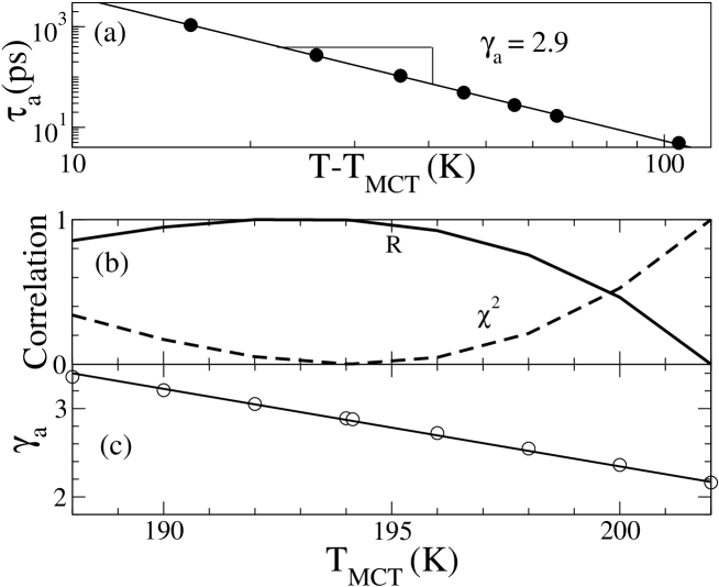
Figure 2: (a) Power law behavior of orientational autocorrelation time $\tau_{a}$ extracted from $C_{1}(t)$, as a function of $T-T_{\rm MCT}$, as predicted by MCT [Eq. (4)]. The line is a fit to the MCT power law with $T_{\rm MCT}=194$ K and exponent $\gamma_{a}=2.9$. (b) To optimize the fit, we vary $T_{\rm MCT}$, calculate the autocorrelation coefficient $R$ (solid line) and the $\chi^{2}$ (dashed line), and choose as our estimate of $T_{\rm MCT}$ the value corresponding to the maximum or minimum of these quantities, within a 10% variation in our range of $T$. $R$ and $\chi^{2}$ are rescaled to the maximum and minimum values we found for 188 K $\leq T_{\rm MCT}\leq$ 202 K. (c) The MCT exponent $\gamma_{a}$ corresponding to different choices of $T_{\rm MCT}$. Note that the exponent $\gamma_{a}$ decreases almost linearly with increasing choice of $T_{\rm MCT}$. Based on the results in (b), our estimates are $T_{\rm MCT}=(194\pm 4)$ K and $\gamma_{a}=2.9\pm 0.3$.

The estimated autocorrelation times $\tau_{a}$ agree (Fig. 2) with the power law behavior predicted by the MCT,

$$\tau_{a}\sim(T-T_{\rm MCT})^{-\gamma_{a}}~{}.$$ (4)

We estimate $T_{\rm MCT}=(194\pm 4)$ K and $\gamma_{a}=2.9\pm 0.3$, in agreement with previous results for similar densities and temperatures MD2 .

The estimated values of $\tau_{a}$, verify well the the von Schweidler law (Appendix) and the time-temperature superposition principle predicted by MCT, i.e. that the autocorrelation functions in the $\alpha$-relaxation regime at different temperatures follow the same master curve if the time is rescaled by the autocorrelation time (Fig. 1b) fabbian .

IV The self-dipole randomization time $\tau_{r}$

IV.1 Definition and Methods

Here we define the randomization time $\tau_{r}$, a new quantity that we propose to characterize the orientational autocorrelation time. We consider the normalized dipole $\vec{\mu}_{i}$ of molecule $i$ over a time interval $\Delta t={\cal N}\delta t$,

$$\bar{\mbox{\boldmath$\mu$}}_{i}\equiv\frac{1}{{\cal N}}\sum_{k=0}^{{\cal N}}\vec{\mu}_{i}(t_{k}),$$ (5)

where $\bar{\mbox{\boldmath$\mu$}}_{i}$ is a function of $\delta t$ and $\Delta t$, $t_{k}\equiv k\delta t$, and $\delta t$ is the time interval between two consecutive samples of $\vec{\mu}_{i}$.

If $\delta t$ is greater than the autocorrelation time of $\vec{\mu}_{i}$, then two consecutive samples $\vec{\mu}_{i}(t)$ and $\vec{\mu}_{i}(t+\delta t)$ are independent, hence $\langle\vec{\mu}_{i}(t_{j})\cdot\vec{\mu}_{i}(t_{k})\rangle=0$ if $j\not=k$, where $\langle....\rangle$ denotes the average over all the molecules $N$ in the system. Hence

$$\langle\bar{\mbox{\boldmath$\mu$}}_{i}^{2}\rangle\equiv\langle\bar{\mbox{\boldmath$\mu$}}_{i}\cdot\bar{\mbox{\boldmath$\mu$}}_{i}\rangle\equiv\frac{1}{{\cal N}^{2}}\langle\sum_{j,k}^{\cal N}\vec{{\mu}}_{i}(t_{j})\cdot\vec{{\mu}}_{i}(t_{k})\rangle=\frac{1}{\cal N},$$ (6)

because $\langle(\vec{{\mu}}_{i})^{2}\rangle=1$ for any $t_{k}$, and

$$\mu_{\rm rms}\equiv\sqrt{\langle\bar{\mbox{\boldmath$\mu$}}_{i}^{2}\rangle}=\frac{1}{\sqrt{\cal N}}=\sqrt{\frac{\delta t}{\Delta t}}~{}~{}.$$ (7)

This is the result of a freely jointed chain of ${\cal N}$ bonds of the same length, for which the mean square end-to-end distance is ${\cal N}^{2}\langle\bar{\mbox{\boldmath$\mu$}}_{i}^{2}\rangle={\cal N}$ feller-flory . Therefore, if $\delta t$ is larger than the orientational autocorrelation time for $\vec{\mu}_{i}$, the $\mu_{\rm rms}$ decreases as $1/\sqrt{\Delta t}$.

If, instead, $\delta t$ is shorter than the orientational autocorrelation time, consecutive elements in the sum in Eq. (6) are correlated $\langle\vec{\mu}_{i}(t)\cdot\vec{\mu}_{i}(t+\delta t)\rangle=z$, resulting in a smaller fluctuation. This can be formally understood by considering the freely rotating chain model feller-flory , where consecutive bonds in the chain are free to rotate, each around the axis of the previous bond, at an angle $\theta$, such that $\cos(\theta)=z$. With this assumption, the resulting mean square end-to-end distance for $n$ bonds of unit length is

$$\langle r_{n}^{2}\rangle=n\frac{1+z}{1-z}-2z\frac{1-z^{n}}{(1-z)^{2}}.$$ (8)

In the case of small $\theta$, we have $z=1-\epsilon+O(\epsilon^{2})$, with $\epsilon=\theta^{2}/2\ll 1$ and $z^{n}\simeq\exp(-n\epsilon)$. Then, from Eq. (8), we obtain

$$\left\langle\frac{1}{n}\sqrt{r_{n}^{2}}\right\rangle=\frac{1}{n\epsilon}\left[2\left({n\epsilon}-1-e^{-n\epsilon}\right)\right]^{1/2}~{}.$$ (9)

In our problem, the bonds are dipole vectors sampled at time intervals $\delta t$, and $n=\Delta t/\delta t={\cal N}$. Therefore Eq. (9) becomes

$$\mu_{\rm rms}\sim\frac{1}{\cal N\epsilon}\left[2\left({\cal N\epsilon}-1-e^{-\cal N\epsilon}\right)\right]^{1/2}~{}.$$ (10)

The right-hand side of this equation behaves as $1/\sqrt{\Delta t}$ for ${\cal N}\rightarrow\infty$, i.e., the random case behavior is recovered for large $\Delta t/\delta t$.

Therefore, if we define $\tau_{r}$ as the time at which the correlation goes to zero as $1/\sqrt{\Delta t}$, it is possible to see that

$$\mu_{\rm rms}\sim 1/\sqrt{\Delta t}\begin{cases}\mbox{ for any }\Delta t&\mbox{if }\delta t\geq\tau_{r}\\ \mbox{ for }\Delta t\gg\tau_{r}&\mbox{if }\delta t<\tau_{r}.\end{cases}$$ (11)

If we consider the fluctuation of any observable, the relation (11) defines the randomization time $\tau_{r}$ for that observable binder and $\tau_{r}$ is equal to the smallest $\delta t$ such that $\mu_{\rm rms}\sim 1/\sqrt{\Delta t}$ for any $\Delta t$.

IV.2 Calculation of $\tau_{r}$

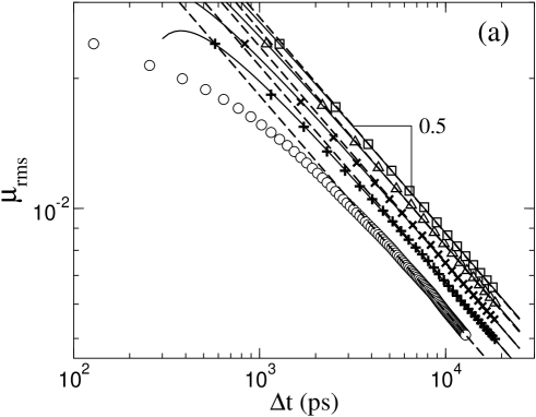
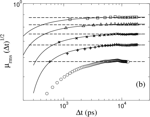
Figure 3: (a) The $\mu_{\rm rms}$ of Eq. (7) for $T=220$ K, plotted versus $\Delta t$ for a range of different time steps $\delta t=128$ ps ($\bigcirc$), 576 ps ($+$), 832 ps ($\times$), 1088 ps ($\bigtriangleup$), and 1280 ps ($\Box$). Dashed lines show the predicted asymptotic behavior $\mu_{\rm rms}\sim 1/\sqrt{\Delta t}$. The fit with Eq. (10) (solid lines) is good when $\delta t\geq 576$ ps, but we are unable to fit the data for $\delta t=128$ ps, showing that the angle between the dipoles in Eq. (6) is not independent, as assumed in the freely rotating chain model. However, Eq. (10) gives a fair description of the approach to the asymptotic regime. (b) $\mu_{\rm rms}\sqrt{\Delta t}$ vs $\Delta t$ approaches a constant asymptotically when $\Delta t\gg\tau_{r}$. In both panels (a) and (b) the errors are roughly the size of the symbols.

In Fig. 3, we show $\mu_{\rm rms}$ for $T=220$ K calculated for different values of $\delta t$. For small $\delta t$ and small $\Delta t$, $\mu_{\rm rms}$ deviates largely from the asymptotic law. However, for increasing $\delta t$, the deviation decreases. For $\delta t=1280$ ps the asymptotic behavior, within the error of our calculations, is reached.

The evaluation of $\tau_{r}$ from a plot such as in Fig. 3 could be problematic, since it depends critically on the data errors. Therefore, to define in a clear way $\tau_{r}$, we fit the first eight points ($\Delta t=\delta t,2\delta t,....,8\delta t$) using

$$\mu_{\rm rms}\sim(\Delta t)^{\lambda},$$ (12)

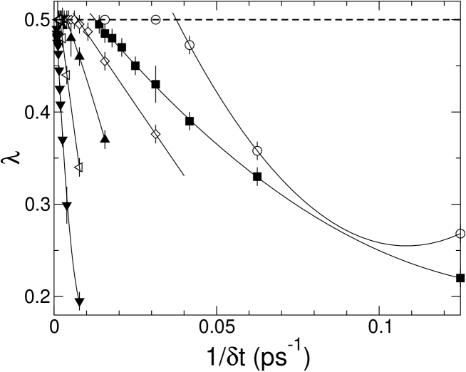
Figure 4: The exponent $\lambda$, defined in Eq. (12) and calculated using the first eight points of the curves in Fig. 3, versus the inverse of time-step $\delta t$, for $T=300$ K ($\bigcirc$), 260 K ($\blacksquare$), 250 K ($\Diamond$), 240 K ($\blacktriangle$), 230 K ($\lhd$), 220 K ($\blacktriangledown$). Where not shown the errors are smaller than the symbol size. The horizontal dashed line corresponds to $\lambda=0.5$. By a quadratic fit of the data with $\lambda<0.5$, we find the self-dipole randomization time $\tau_{r}$, defined as the value of $\delta t$ where $\lambda=1/2$.

where $\lambda=\lambda(\delta t)$. In this way we study how the deviation from the asymptotic regime decreases by increasing $\delta t$. We find that the exponent $\lambda$ increases toward the asymptotic value $1/2$ for increasing $\delta t$, and $\lambda=1/2$ for any $\delta t\geq\tau_{r}$ (Fig. 4). We therefore define $\tau_{r}$ as the extrapolated values of $\delta t$ at which $\lambda=1/2$. We find that $\lambda$ approaches 1/2 as $1/\delta t$, to the leading order, for low temperatures (Fig. 4).

The resulting values of $\tau_{r}$ are presented in Fig.5a as functions of $T-T_{\rm MCT}$, showing that the power law behavior Eq. (4) is well satisfied by $\tau_{r}$. In this case our estimates are $T_{\rm MCT}=(191.5\pm 2.5)$ K and $\gamma_{r}=3.3\pm 0.2$, both consistent within the errors with the estimates based on $\tau_{a}$ (Fig.2). Therefore, the prediction (i) of MCT is verified.

By plotting $\tau_{r}$ against $\tau_{a}$, we verify the MCT prediction (ii). We find (Fig. 6) that $\tau_{r}$ and $\tau_{a}$ are linearly related and that $\tau_{r}$ is approximately five times larger than $\tau_{a}$.

The large value of $\tau_{r}$ with respect to $\tau_{a}$ is consistent with the fact that the latter measures the decay of the self-dipole correlation to a finite value, while the first measures the time needed for the self-dipole autocorrelation to decay to zero. This result is also reminiscent of the recent MD analysis in bulk water for the site-dipole field, a measure of the average orientation of the molecules passing through each spatial position, recently introduced in Ref.  masaki . Higo et al. masaki find coherent patterns for the site-dipole field, at ambient pressure and $T=298$ K and $T=300$ K, that persist for more than 100 ps, a time much larger than the single molecule orientational relaxation time $\tau_{a}$ of approximately 5 ps (Table I). It is, therefore, interesting to calculate the randomization time $\tau_{\rm box}$ and to find its relation with the autocorrelation time $\tau_{a}$ for $T\to T_{\rm MCT}$.

V The site-dipole field

To check if there are large correlated domains of dipoles in water which have large relaxation times compared to the individual dipole correlation time, we next study site-dipole field introduced by Higo et. al. masaki . We define the instantaneous coarse-grained site-dipole field

$$\vec{d}^{v}_{i}\equiv\vec{d}(\vec{r_{i}},t)\equiv\frac{1}{n_{i}(t)}\sum_{\rm box}\vec{\mu}_{i}$$ (13)

as the average of dipoles $\vec{\mu}_{i}$ of all the molecules $n_{i}(t)$ at time $t$ belonging to box $i$ of edge $L_{\rm box}$, volume ${v}=L^{3}_{\rm box}$ and centered at $\vec{r_{i}}$. If $n_{i}(t)=0$, then $\vec{d}^{v}_{i}=0$ by definition note2 ; mathias . We chose vectors $\vec{r_{i}}$ in such a way that the corresponding boxes do not overlap note1 . The time average $\bar{d}^{v}_{i}$ over an interval $\Delta t$, is defined analogously to Eq. (5). The rms average $d^{v}_{{\rm rms}}$, is defined in analogy to Eq. (6) and (7), but instead of summation over all molecules we perform a summation over all boxes.

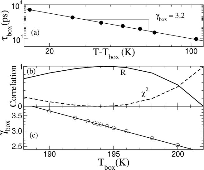
Figure 7: Analog of Fig. 2 and Fig. 6 for the site-dipole randomization time $\tau_{\rm box}$. (a) We find a power law behavior in $T-T_{\rm box}$, calculated for $L_{\rm box}=3$Å. The line is a fit with $T_{\rm MCT}=194$ K and exponent $\gamma_{\rm box}=3.2$. (b) Optimization analysis for $T_{\rm box}$: correlation coefficient $R$ (solid line) and $\chi^{2}$ (dashed line), both rescaled to the maximum and minimum values found for $188$ K$\leq T_{\rm box}\leq 202$ K. (c) The exponent $\gamma_{\rm box}$ corresponding to different choices of $T_{\rm box}$, decreases linearly with increasing choice of $T_{\rm box}$. We estimate $T_{\rm box}=(194\pm 2)$ K and $\gamma_{\rm box}=3.2\pm 0.2$.

Since the argument presented for $\mu_{\rm rms}$ is also valid for $d^{v}_{{\rm rms}}$, the relation (11) also holds for $d^{v}_{{\rm rms}}$ and allows us to estimate the randomization time $\tau_{\rm box}$ for $d^{v}_{{\rm rms}}$. We find that $\tau_{\rm box}$, calculated for $L_{\rm box}=3.33$Å , diverges at $T_{\rm box}=(194\pm 2)$ K with a power law with exponent $\gamma_{box}=3.2\pm 0.2$, consistent with our estimates of $\gamma_{a}$ and $T_{\rm MCT}$, respectively (Fig. 7).

If we compare $\tau_{\rm box}$ with $\tau_{r}$ (Fig. 8), we again find a linear relation, as in Fig. 6 for $\tau_{a}$, consistent with the MCT statement (ii). The proportionality factor is approximately 2.5 note3 , smaller than the factor $\approx 5$ found for $\tau_{r}$ in Fig. 6. Therefore, we conclude that in bulk water the coarse-grained site-dipole randomization time $\tau_{\rm box}$ is larger than the self-dipole autocorrelation time $\tau_{a}$, but smaller than $\tau_{r}$. Thus we do not find a significant increase in the box dipole autocorrelation time compared to the autocorrelation time $\tau_{a}$. These results do not support the results of Refs. shelton ; masaki .

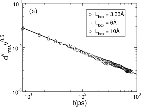
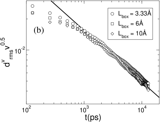
Figure 9: Size dependence of site-dipole autocorrelation function $d^{v}_{\rm rms}$ as a function of $t$ for $L_{\rm box}=3.33$ Å  ($\bigcirc$), 6 Å  ($\Box$), 10 Å  ($\Diamond$) and for two different temperatures (a) $T=300$ K and (b) $T=220$ K. In (a) the line is a fit of data for $L_{\rm box}=3.33$ Å  with $d^{v}_{\rm rms}=a/\sqrt{t}$, with $a=0.08\pm 0.01$. In (b) the same fit is for the data at $L_{\rm box}=6$ Å  and $t>10^{2}$, with $a=0.49\pm 0.01$. For each $T$ all the values of $d^{v}_{\rm rms}\sqrt{v}$ overlap, suggesting that the orientational autocorrelation is short-range.

To test the existence of cooperative domains in the SPC/E model, we perform coarse-graining of the dipole field for boxes of sizes $3.33$ Å $\leq L_{\rm box}\leq 10$ Å. If the dipoles of molecules in the box are independent random variables, $d^{v}_{\rm rms}$ must be inversely proportional to $\sqrt{<n_{i}>}\propto\sqrt{v}$, since the average number of molecules in the box is proportional to its volume. The dependence of $d^{v}_{\rm rms}\sqrt{v}$ on time $t$ must be the same for the boxes of different volumes $v$. We show in Fig. 9 the behavior of $d^{v}_{\rm rms}\sqrt{v}$ for $T=220$ K and $T=300$ K. The collapse of all the curves confirms the hypothesis of very weak autocorrelations among neighboring dipoles. Only for $T=220$ K we observe a weak size dependence of $d^{v}_{\rm rms}\sqrt{v}$ for the smallest size, suggesting that at this $T$ the correlation length is between $3.33$ and $6$ Å, comparable to the dipole-dipole correlation length at ambient $T$ mathias . Thus our simulations support the existence of only short range orientational autocorrelation in SPC/E water even at low $T$.

VI Discussion

Considerable numerical evidence shows that MCT predictions apply to orientational dynamics of water, despite the fact that MCT has been developed for particles interacting through spherically symmetric potentials MCT . However, recent extensions of MCT to liquids of linear molecules Schilling97 ; Kammerer97 , and single solute molecules in a simple solvent liquid orientational , confirm the main MCT predictions about the orientational autocorrelation functions MMCT .

Our study of supercooled water confirms the validity of MCT predictions for the orientational autocorrelation time $\tau_{a}$, estimated through a stretched exponential of the dipole autocorrelation function, for the temperature range $210$ K$\leq T\leq 300$ K at density $\rho=1$ g/cm³. Our results agree with the time-temperature superposition principle and the power law Eq. (4), with $T_{\rm MCT}=(194\pm 4)$ K and $\gamma_{a}=2.9\pm 0.3$.

By evaluating the randomization time $\tau_{r}$, defined as the time needed to randomize the molecular dipoles, we verify the MCT prediction that all the characteristic times of quantities coupled to density fluctuations of a supercooled liquid are proportional to each other and follow the same power law Eq. (4). We find $\tau_{r}\approx 5~{}\tau_{a}$, with $T_{\rm MCT}=(191.5\pm 2.5)$ K and $\gamma_{r}=3.3\pm 0.2$, consistent with the estimates based on the calculation of $\tau_{a}$.

We also calculate the randomization time $\tau_{\rm box}$ for the box dipole field, a quantity introduced in Ref. masaki to measure the local orientational memory of molecules passing through a given spatial position. Our results for $L_{\rm box}=3.33$ Åshow that $\tau_{\rm box}$ diverges at $T_{\rm box}=T_{\rm MCT}$, following a power law with exponent $\gamma_{\rm box}=\gamma_{a}$, and that $\tau_{\rm box}\approx\tau_{r}/2$. As a consequence, the local memory is lost faster than the self-dipole orientational memory.

Our results also show the existence of domains of correlated dipoles of short spatial range, with a correlation length comparable to the dipole-dipole correlation length at ambient $T$ mathias . Whether this conclusion is specific to the SPC/E model with reaction field is an open question, and requires further investigation using other models of water, e.g. polarizable models.

Acknowledgments

We thank N. Giovambattista for his helpful collaboration on initial phase of this work. We thank the NSF Chemistry Program for support. GF thanks the Spanish Ministerio de Educación y Ciencia (Programa Ramón y Cajal and Grant No. FIS2004-03454), and M. Sasai for his hospitality during a visit to Nagoya University.

Appendix A The von Schweidler law

The MCT predicts that the autocorrelation function departs from the plateau $A$ as a power law with exponent $b$, known as the von Schweidler law,

$$C_{1}(t)-A\sim-(t/\tau_{a})^{b}~{},$$ (14)

where the von Schweidler exponent $b$ does not depend on $T$. We verify that at lower temperatures Eq. (14) holds for roughly two decades in time (Fig. 10) and we find a clear deviation only for $T\geq 260$ K at short times, possibly due to the fact that for $T\geq 260$ K it is more difficult to estimate the plateau $A$. The estimated value of $b$ is $0.6\pm 0.1$, consistent with previous results fabbian and with the MCT prediction that $\gamma_{a}$, $a$, and $b$ are related by the equation

$$\gamma_{a}=\frac{1}{2a}+\frac{1}{2b}.$$ (15)

Here $a$ is the exponent of the power law that describes the short-time approach to the plateau $C_{1}-A\sim t^{-a}$, and $a$ is related to $b$ by the transcendental equation

$$\frac{[\Gamma(1-a)]^{2}}{\Gamma(1-2a)}=\frac{[\Gamma(1+b)]^{2}}{\Gamma(1+2b)},$$ (16)

where $\Gamma(x)$ is the Euler gamma function. Our estimates of $b$ and $\gamma_{a}$ are consistent with both Eqs. (15) and (16) with $a=0.25\pm 0.05$.

The values of the exponents $a$, $b$ and $\gamma_{a}$ are not universal, but depend on density. However, the rescaling of the autocorrelation functions for different $T$ on the same master curve, shows that the orientational correlation function depends on $T$ and $\rho$ only through the dependence on $\tau_{a}$, as predicted by the MCT.

Table 1: Parameters of the fit of $C_{1}(t)$ in Fig. 1 with Eq. (1). The error on each parameter is $\pm 10\%$.

$T($K$)$	$A$	$\tau_{a}($ps$)$	$\beta$
300	0.93	$4.9\times 10^{0}$	0.88
260	0.94	$1.7\times 10^{1}$	0.85
250	0.94	$2.8\times 10^{1}$	0.85
240	0.94	$4.9\times 10^{1}$	0.84
230	0.94	$1.1\times 10^{2}$	0.84
220	0.94	$2.7\times 10^{2}$	0.83
210	0.94	$1.1\times 10^{3}$	0.82

Figure 1: (a) The orientational autocorrelation function $C_{1}$ as a function of time $t$ for $T(K)=210$ ($\bigcirc$), 220 ($\Box$), 230 ($\Diamond$), 240 ($\bigtriangleup$), 250 ($\lhd$), 260 ($\bigtriangledown$), 300($\rhd$). Symbols are simulations, lines are fits over the range for $t\geq 0.03$ ps to Eq. (1) with the fitting parameters listed in Table 1. (b) Test of the time-temperature superposition principle, as predicted by MCT. The symbols and the lines for different $T$ fall on a single curve if the times are rescaled by $\tau_{a}(T)$.

Figure 5: Analog of Fig. 2 for the self-dipole randomization time $\tau_{r}$. (a) $\tau_{r}$ follows a power law behavior in $T-T_{\rm MCT}$ [Eq. (4)], as predicted by MCT. The line is a fit with $T_{\rm MCT}=191.5$ K and power $\gamma_{r}=3.3$. (b) As in Fig. 2, to optimize the estimate of $T_{\rm MCT}$ we calculate the autocorrelation coefficient $R$ (solid line) and the $\chi^{2}$ (dashed line). In (b), $R$ and $\chi^{2}$ are rescaled to the maximum and minimum values we found for 187 K $\leq T_{\rm MCT}\leq$ 200 K. (c) The fitting parameter $\gamma_{r}$ corresponding to different estimates of $T_{\rm MCT}$. The exponent $\gamma_{r}$ decreases linearly with increasing estimates of $T_{\rm MCT}$. Based on the results in (b), our estimates are $T_{\rm MCT}=(191.5\pm 2.5)$ K and $\gamma_{r}=3.3\pm 0.2$.

Figure 6: Parametric plot of the times $\tau_{r}(T)$ and $\tau_{a}(T)$, within the range $220$ K $\leq T\leq 300$ K, with the lowest time corresponding to the highest $T$. The line reflects the linear one-parameter fit, $\tau_{r}=(5.1\pm 0.2)\tau_{a}$.

Figure 8: Analog of Fig. 7: A parametric plot of the site-dipole randomization time $\tau_{\rm box}(T)$ and the orientational autocorrelation time $\tau_{a}(T)$ over the range $220$ K $\leq T\leq 300$ K, with the lowest time corresponding to the highest $T$. The line reflects the linear one-parameter fit $\tau_{\rm box}=(2.5\pm 0.2)\tau_{a}$.

Figure 10: Test of the von Schweidler law, Eq. (14). It is well verified roughly over two decades, for $T\leq 250$ K. Data for higher $T$ depart from this law at short times. Symbols are as in Fig. 1. Dashed line is the fit to Eq. (14) of the data for $T=230$ K over the fitting range $0.01\leq A-C_{1}\leq 0.50$ with the result $b=0.6\pm 0.1$.

References

- (1) See, e.g., M.-C. Bellissent-Funel, ed., Hydration Processes in Biology: Theoretical and Experimental Approaches (IOS Press, Amsterdam, 1999); P. G. Debenedetti, J. Phys. Cond. Matt. 15, R1669 (2003); P. G. Debenedetti and H. E. Stanley, Physics Today 56 [issue 6], 40–46 (2003); O. Mishima and H. E. Stanley, Nature 396, 329–335 (1998).
- (2) G. Sposito, J. Chem. Phys. 74, 6943 (1981).
- (3) S. H. Chen, J. Teixeira, and R. Nicklow, Phys. Rev. A 26, 3477 (1982).
- (4) F. X. Prielmeir, E. W. Lang, R. J. Speedy, and H. D. Lüdeman, Phys. Rev. Lett. 59, 1128 (1987).
- (5) C. A. Angell, Nature 331, 206 (1988).
- (6) V. Mazzacurati, A. Nucara, M. A. Ricci, G. Ruocco, and G. Signorelli, J. Chem. Phys. 93, 7767 (1990).
- (7) F. Sobron, F. Puebla, F. Rull, and O. F. Nielsen, Chem. Phys. Lett. 185, 393 (1991).
- (8) K. Mizoguchi, Y. Hori, and Y. Tominaga, J. Chem. Phys. 97, 1961 (1992).
- (9) S.-H. Chen, in Hydrogen-Bonded Liquids, Vol. 329 of NATO Advanced Studies Institute Series, edited by J. C. Dore and J. Teixeira (Kluwer Academic, Dordrecht, 1991), pp. 289–332; S. Dellerue and M.-C. Bellissent-Funel, Chem. Phys. 258, 315 (2000); A. R. Bizzarri and S. Cannistraro, J. Phys. Chem. B 106, 6617 (2002).
- (10) S.-H. Chen, P. Gallo, and M.-C. Bellissent Funel, Can. J. Phys. 73, 703 (1995).
- (11) M.-C. Bellissent-Funel, S.-H. Chen, and J.-M. Zanotti, Phys. Rev. E 51, 4558 (1995).
- (12) J.-M. Zanotti, M.-C. Bellissent-Funel, and S.-H. Chen, Phys. Rev. E 59, 3084 (1999).
- (13) S. Takahara, M. Nakano, S. Kittaka, Y. Kuroda, T. Mori, H. Hamano, and T. Yamaguchi, J. Phys. Chem. 103, 5814 (1999).
- (14) J. T. Cabral, A. Luzar, J. Teixeira, and M.-C. Bellissent-Funel, J. Chem. Phys. 113, 8736 (2000).
- (15) V. Crupi, D. Majolino, P. Migliardo, and V. Venuti, J. Phys. Chem. A 104, 11000 (2000).
- (16) V. Crupi, D. Majolino, P. Migliardo, and V. Venuti, J. Chem. Phys. B 106, 10884 (2002).
- (17) S. Magazu and G. Maisano, J. Mol. Liq. 93, 7 (2001).
- (18) Y. Xie, K. F. Ludwig, Jr., G. Morales, D. E. Hare, and C. M. Sorensen, Phys. Rev.Lett. 71, 2050 (1993).
- (19) L. Bosio, J. Teixeira, and H. E. Stanley, Phys. Rev. Lett. 46, 597 (1981).
- (20) J. Teixeira, M.-C. Bellissent-Funel, S.-H. Chen, and A. J. Dianoux, Phys. Rev. A 31, 1913 (1985).
- (21) D. P. Shelton, Phys. Rev. B, 72, 020201 (2005).
- (22) P. Gallo, F. Sciortino, P. Tartaglia, and S.-H. Chen, Phys. Rev. Lett. 76, 2730 (1996).
- (23) F. Sciortino, P. Gallo, P. Tartaglia, and S.-H. Chen, Phys. Rev. E 54, 6331 (1996).
- (24) F. W. Starr, S. Harrington, F. Sciortino, H. E. Stanley, Phys. Rev. Lett. 82, 3629 (1999); F. W. Starr, F. Sciortino, and H. E. Stanley, Phys. Rev. E 60, 6757 (1999).
- (25) D. Paschek and A. Geiger, J. Phys. Chem. B 103, 4139 (1999); P. Gallo, M. Rovere, and E. Spohr, Phys. Rev. Lett. 85, 4317 (2000).
- (26) P. A. Netz, F. W. Starr, H. E. Stanley, and M. C. Barbosa, J. Chem. Phys. 115, 344 (2001); P. A. Netz, F. W. Starr, M. C. Barbosa, and H. E. Stanley, J. Mol. Liq. 101, 159 (2002).
- (27) S.-H. Chen, C. Liao, F. Sciortino, P. Gallo, and P. Tartaglia, Phys. Rev. E 59, 6708 (1999); C. Y. Liao, F. Sciortino, and S. H. Chen, Phys. Rev. E 60, 6776 (1999).
- (28) D. Di Cola, A. Deriu, M. Sampoli, and A. Torcini, J. Chem. Phys. 104, 4223 (1996); S.-H. Chen, P. Gallo, F. Sciortino, and P. Tartaglia, Phys. Rev. E 56, 4231 (1997).
- (29) F. Sciortino, L. Fabbian, S. H. Chen, and P. Tartaglia, Phys. Rev. E 56, 5397 (1997); L. Fabbian, F. Sciortino, and P. Tartaglia, J. Non-Cryst. Solids 235-237, 350 (1998).
- (30) A. Faraone, L. Liu, C. Y. Mou, P. C. Shih, J. R. D. Copley, and S.-H. Chen, J. Chem. Phys. 119, 3963 (2003).
- (31) L. Liu, A. Faraone, and S.-H. Chen, Phys. Rev. E 65, 041506 (2002).
- (32) L. Fabbian, F. Sciortino, F. Thiery, and P. Tartaglia, Phys. Rev. E 57, 1485 (1998); L. Fabbian, R. Schilling, F. Sciortino, P. Tartaglia, and C. Theis, Phys. Rev. E 58, 7272 (1998); L. Fabbian, F. Sciortino, and P. Tartaglia, Phil. Mag. B 77, 499 (1998).
- (33) L. Fabbian, A. Latz, R. Schilling, F. Sciortino, P. Tartaglia, and C. Theis, Phys. Rev. E 62, 2388 (2000).
- (34) A. Faraone, L. Liu, and S.-H. Chen, J. Chem. Phys. 119, 6302 (2003).
- (35) J. Higo, M. Sasai, H. Shirai, H. Nakamura, and T. Kugimiya, Proc. Nat. Acad. Sci. 98, 5961 (2001).
- (36) Y.-L. Yhe and C.-Y. Mou, J. Phys. Chem B 103, 3699 (1999).
- (37) See, e.g., K. Binder, ed., Monte Carlo Methods in Statistical Physics (Springer-Verlag, Berlin, 1979).
- (38) H. J. C. Berendsen, J. R. Grigera, and T. P. Stroatsma, J. Phys. Chem. 91, 6269 (1987).
- (39) Microwave spectroscopy and infrared spectroscopy on H2O at equilibrium in the gas phase give 0.9575Å for the O-H distance and 104.51o for the HOH angle [D. R. Lide CRC Handbook of Chemistry and Physics, 84th Edition (CRC Press, Boca Raton FL, 2003)].
- (40) H. J. C. Berendsen, J. P. M. Postma, W. F. van Gunsteren, A. DiNola, and J. R. Haak, J. Phys. Chem. 81, 3684 (1984).
- (41) O. Steinhauser, Mol. Phys. 45, 335 (1982).
- (42) W. Feller, An Introduction to Probability Theory and Its Applications, Vol. 1, 2nd Edition (John Wiley & Sons, New York, 1960), pp. 225–226; P. J. Flory, Statistical Mechanics of Chain Molecules (John Wiley & Sons, New York, 1969), p. 16.
- (43) In Eq. (13) we normalize the average with the time-dependent number of molecules , instead of the total number of cells inside the box as in Ref. masaki . Our choice has the advantage of giving rise to a value of the average dipole in a box independent of the system density (see for example mathias ). However, as a consequence, the distribution of is not Gaussian, as would be expected by normalizing by a constant factor. We have verified that by using a constant normalization factor we recover a Gaussian distribution. Moreover, we have verified that our final results are not affected by the choice of the normalization factor in Eq. (13).
- (44) G. Mathias and P. Tavan, J. Chem. Phys. 120, 4393 (2004).
- (45) The definition in Eq. (13) differs from the one introduced in Ref. masaki , where the coarse-grained site-dipole field is averaged over spheres with radius and centered at a distance shorter than . The definition in Ref. masaki emphasizes the spatial-patterns of coarse-grained site-dipoles, because each molecular dipole contributes to the coarse-grained site-dipole for all the (overlapping) spheres which contain the same molecule. We therefore expect to find patterns that survive for a time shorter than that measured in Ref. masaki . Indeed, we do not find strong evidence of surviving patterns in bulk water within our time resolution.
- (46) At K we find a autocorrelation time approximately 10 times smaller than the persistence time found in Ref. masaki for the site-dipoles patterns. This is due to the difference in the definition in Eq. (13). We verify that, by adopting the same definition of Ref. masaki , we can reproduce the bulk-water results of Higo et al. See also note1 .
- (47) See for example W. Götze, J. Phys.: Condens. Matter 11, A1 (1999); W. Götze and L. Sjogren, Rep. Prog. Phys. 55, 241 (1992); E. Leutheusser, Phys. Rev. A 29, 2765 (1984); W. Götze, in Liquids, Freezing and the Glass Transition, Proceedings of the Les Houches Summer School of Theoretical Physics, Session LI, 1989, edited by J. P. Hansen, D. Levesque, and J. Zinn-Justin (North-Holland, Amsterdam, 1991); A. P. Sokolov, J. Hurst, and D. Quitmann, Phys. Rev. B 51, 12 865 (1995).
- (48) R. Schilling and T. Scheidsteger, Phys. Rev. E 56, 2932 (1997).
- (49) S. Kammerer, W. Kob, and R. Schilling, Phys. Rev. E 56, 5450 (1997).
- (50) T. Franosch, M. Fuchs, W. Götze, M. R. Mayr, and A. P. Singh, Phys. Rev. E 56, 5659 (1997); W. Götze, A. P. Singh, and T. Voigtmann, Phys. Rev. E 61, 6934 (2000); S.-H. Chong and W. Götze, Phys. Rev. E 65, 051201 (2002); Phys. Rev. E 65, 041503 (2002).