Time-Dependent Density Functional Theory with Ultrasoft Pseudopotential: Real-Time Electron Propagation across Molecular Junction

Abstract

A practical computational scheme based on time-dependent density functional theory (TDDFT) and ultrasoft pseudopotential (USPP) is developed to study electron dynamics in real time. A modified Crank-Nicolson time-stepping algorithm is adopted, under planewave basis. The scheme is validated by calculating the optical absorption spectra for sodium dimer and benzene molecule. As an application of this USPP-TDDFT formalism, we compute the time evolution of a test electron packet at the Fermi energy of the left metallic lead crossing a benzene-(1,4)-dithiolate junction. A transmission probability of 5-7%, corresponding to a conductance of 4.0-5.6 $\mu$S, is obtained. These results are consistent with complex band structure estimates, and Green’s function calculation results at small bias voltages.

I Introduction

The development of molecular scale electronic devices has attracted a great deal of interest in the past decade, although major experimental and theoretical challenges still exist. Reed et al. (1997); Smit et al. (2002); Joachim et al. (2000); Nitzan (2001); Heath and Ratner (2003) To date precise experimental control of molecular conformation is lacking, resulting in large uncertainties in the measured conductance. On the theory side, while the Green’s function (GF) method has achieved many successes in describing electron transport at the meso Datta (1995); Imry (2002) and molecular Derosa and Seminario (2001); Damle et al. (2001); Taylor et al. (2001); Xue and Ratner (2003); Ke et al. (2004) scales, issues such as dynamical electron correlation and large electron-phonon coupling effects Galperin et al. (2005a, b) are far from fully resolved. It is therefore desirable to exploit alternative approaches for comparison with the mainstream GF calculations. In this paper, we describe a first step towards this goal by computing how an electron propagates through a molecular junction in real time, based on the time-dependent density functional theory Runge and Gross (1984) (TDDFT).

Density functional theory (DFT) Hohenberg and Kohn (1964) with the Kohn-Sham reference kinetic energy functional of a fictitious non-interacting electron system Kohn and Sham (1965) is a leading method for treating many electrons in solids and molecules. Parr and Yang (1989). While initially formulated to describe only the electronic ground state Hohenberg and Kohn (1964); Kohn and Sham (1965), it has been rigorously extended by Runge and Gross Runge and Gross (1984) to treat time-dependent, driven systems (excited states). TDDFT is therefore a natural theoretical platform for studying electron conduction at the nanoscale. There are two flavors in which TDDFT is implemented. One is direct numerical integration Yabana and Bertsch (1996, 1999); Bertsch et al. (2000); Marques et al. (2003); Tsolakidis et al. (2002); Castro et al. (2004) of the time-dependent Kohn-Sham (TDKS) equations. The other is a Gedanken experiment of the former with an added assumption of infinitesimal time-dependent perturbation, so a linear response function may be first derived in closed form Bauernschmitt and Ahlrichs (1996); Casida et al. (1998); Chelikowsky et al. (2003), which is then evaluated numerically. These two implementations should give exactly the same result when the external perturbation field is infinitesimal. The latter implementation can be computationally more efficient once the linear-response function has been analytically derived, while the former can treat non-infinitesimal perturbations and arbitrary initial states.

A key step of the TDDFT dynamics is updating of the Kohn-Sham effective potential by the present excited-state charge density $\rho({\bf x},t)$, $\hat{V}_{\rm KS}(t)=\hat{V}_{\rm KS}[\rho({\bf x},t),...]$. This is what sets TDDFT apart from the ground-state DFT estimate of excitation energies, even when TDDFT is applied in its crudest, so-called adiabatic approximation, Bauernschmitt and Ahlrichs (1996) whereby the same exchange-correlation density functional form as the ground-state DFT calculation is used (for example, the so-called TDLDA approximation uses exactly the same Ceperley-Alder-Perdew-Zunger functional Ceperley and Alder (1980); Perdew and Zunger (1981) as the ground-state LDA calculation.) This difference in excitation energies comes about because in a ground-state DFT calculation, a virtual orbital such as LUMO (lowest unoccupied molecular orbital) experiences an effective potential due to $N$ electrons occupying the lowest $N$ orbitals; whereas in a TDDFT calculation, if one electron is excited to a LUMO-like orbital, it sees $N-1$ electrons occupying the lowest $N-1$ orbitals, plus its own charge density. Also, the excitation energy is defined by the collective reaction of this coupled dynamical system to time-dependent perturbation (pole in the response function) Li and Yip (1997), rather than simple algebraic differences between present virtual and occupied orbital energies. For rather involved reasons beyond what is discussed here, TDDFT under the adiabatic approximation gives significantly improved excitation spectra Bauernschmitt and Ahlrichs (1996); Casida et al. (1998), although there are still much to be desired. Further systematic improvements to TDDFT such as current density functional Vignale and Kohn (1996) and self-interaction correction Tong and Chu (1998) have already made great strides.

Presently, most electronic conductance calculations based on the Landauer transmission formalism Landauer (1957, 1970) have assumed a static molecular geometry. In the Landauer picture, dissipation of the conducting electron energy is assumed to take place in the metallic leads (electron reservoirs), not in the narrow molecular junction (channel) itself. Imry and Landauer (1999) Inelastic scattering, however, does occur in the molecular junctions themselves, the effects appearing as peaks or dips in the measured inelastic electron tunneling spectra (IETS) Galperin et al. (2004) at molecular vibrational eigen-frequencies. Since heating is always an important concern for high-density electronics, and because molecular junctions tend to be mechanically more fragile compared to larger, semiconductor-based devices, the issue of electron-phonon coupling warrants detailed calculations Galperin et al. (2004); Frederiksen et al. (2004) (here we use the word phonon to denote general vibrations when there is no translational symmetry). In the case of long $\pi$-conjugated polymer chain junctions, strong electron-phonon coupling may even lead to new elementary excitations and spin or charge carriers, called soliton/polaron Heeger et al. (1988); Galperin et al. (2005a, b); Lin et al. (2005a, b), where the electronic excitation is so entangled with phonon excitation that separation is no longer possible.

In view of the above background, there is a need for efficient TDDFT implementations that can treat complex electron-electron and electron-phonon interactions in the time domain. Linear-response type analytic derivations can become very cumbersome, and for some problems Calvayrac et al. (2000) may be entirely infeasible. A direct time-stepping method Yabana and Bertsch (1996, 1999); Bertsch et al. (2000); Marques et al. (2003); Castro et al. (2004); Tsolakidis et al. (2002) analogous to molecular dynamics for electrons as well as ions may be more flexible and intuitive in treating some of these highly complex and coupled problems, if the computational costs can be managed. Such a direct time-stepping code also can be used to double-check the correctness of analytic approaches such as the non-equilibrium Green’s function (NEGF) method and electron-phonon scattering calculations Galperin et al. (2004); Frederiksen et al. (2004), most of which explicitly or implicitly use the same set of TDDFT approximations (most often an adiabatic approximation such as TDLDA).

Two issues are of utmost importance when it comes to computational cost: choice of basis and pseudopotential. For ground-state DFT calculations that involve a significant number of metal atoms (e.g. surface catalysis), the method that tends to achieve the best cost-performance compromise is the ultrasoft pseudopotential (USPP) Vanderbilt (1990); Laasonen et al. (1991, 1993) with planewave basis, and an independent and theoretically more rigorous formulation, the projector augmented-wave (PAW) Blochl (1994) method. Compared to the more traditional norm-conserving pseudopotential approaches, USPP/PAW achieve dramatic cost savings for first-row $p$- and $d$-elements, with minimal loss of accuracy. USPP/PAW are the workhorses in popular codes such as VASP Kresse and Furthmuller (1996) and DACAPO DAC (web site); Hammer et al. (1999); Bahn and Jacobsen (2002). We note that similar to surface catalysis problems, metal-molecule interaction at contact is the key for electron conduction across molecular junctions. Therefore it seems reasonable to explore how TDDFT, specifically TDKS under the adiabatic approximation, performs in the USPP/PAW framework, which may achieve similar cost-performance benefits. This is the main distinction between our approach and the software package Octopus Marques et al. (2003); Castro et al. (2004), a ground-breaking TDDFT program with direct time stepping, but which uses norm-conserving Troullier-Martins (TM) pseudopotential Troullier and Martins (1991), and real-space grids. We will address the theoretical formulation of TD-USPP (TD-PAW) in sec. II, and the numerical implementation of TD-USPP in the direct time-stepping flavor in sec. III.

To validate that the direct time-integration USPP-TDDFT algorithm indeed works, we calculate the optical absorption spectra of sodium dimer and benzene molecule in sec. IV and compare them with experimental results and other TDLDA calculations. As an application, we perform a computer experiment in sec. V which is a verbatim implementation of the original Landauer picture Landauer (1970); Imry and Landauer (1999). An electron wave pack comes from the left metallic lead (1D Au chain) with an energy that is exactly the Fermi energy of the metal (the Fermi electron), and undergoes scattering by the molecular junction (benzene-(1,4)-dithiolate, or BDT). The probability of electron transmission is carefully analyzed in density vs. ${\bf x},t$ plots. The point of this exercise is to check the stability and accuracy of the time integrator, rather than to obtain new results about the Au-BDT-Au junction conductance. We check the transmission probability thus obtained with simple estimate from complex band structure calculations Tomfohr and Sankey (2002a, b), and Green’s function calculations at small bias voltages. Both seem to be consistent with our calculations. Lastly, we give a brief summary in sec. VI.

II TDDFT formalism with ultrasoft pseudopotential

The key idea of USPP/PAW Vanderbilt (1990); Laasonen et al. (1991, 1993); Blochl (1994) is a mapping of the true valence electron wavefunction $\tilde{\psi}({\bf x})$ to a pseudowavefunction $\psi({\bf x})$: $\tilde{\psi}\leftrightarrow\psi$, like in any pseudopotential scheme. However, by discarding the requirement that $\psi({\bf x})$ must be norm-conserved ($\langle\psi|\psi\rangle=1$) while matching $\tilde{\psi}({\bf x})$ outside the pseudopotential cutoff, a greater smoothness of $\psi({\bf x})$ in the core region can be achieved; and therefore less planewaves are required to represent $\psi({\bf x})$. In order for the physics to still work, one must define augmentation charges in the core region, and solve a generalized eigenvalue problem

$$\hat{H}|\psi_{n}\rangle=\varepsilon_{n}\hat{S}|\psi_{n}\rangle,$$ (1)

instead of the traditional eigenvalue problem, where $\hat{S}$ is a Hermitian and positive definite operator. $\hat{S}$ specifies the fundamental measure of the linear Hilbert space of pseudowavefunctions. Physically meaningful inner product between two pseudowavefunctions is always $\langle\psi|\hat{S}|\psi^{\prime}\rangle$ instead of $\langle\psi|\psi^{\prime}\rangle$. For instance, $\langle\psi_{m}|\psi_{n}\rangle\neq\delta_{mn}$ between the eigenfunctions of (1) because it is actually not physically meaningful, but $\langle\psi_{m}|\hat{S}|\psi_{n}\rangle\equiv\langle\tilde{\psi}_{m}|\tilde{\psi}_{n}\rangle=\delta_{mn}$ is. (Please note that $\tilde{\psi}$ is used to denote the true wavefunction with nodal structure, and ${\psi}$ to denote pseudowavefunction, which are opposite in some papers.)

$\hat{H}$ consists of the kinetic energy operator $\hat{T}$, ionic local pseudopotential $\hat{V}_{\rm L}$, ionic nonlocal pseudopotential $\hat{V}_{\rm NL}$, Hartree potential $\hat{V}_{\rm H}$, and exchange-correlation potential $\hat{V}_{\rm XC}$,

$$\hat{H}=\hat{T}+\hat{V}_{\rm L}+\hat{V}_{\rm NL}+\hat{V}_{\rm H}+\hat{V}_{\rm{XC}}.$$ (2)

The $\hat{S}$ operator is given by

$$\hat{S}=1+\sum_{i,j,I}q_{ij}^{I}|\beta_{j}^{I}\rangle\langle\beta_{i}^{I}|,$$ (3)

where $i\equiv(\tau lm)$ is the angular momentum channel number, and $I$ labels the ions. $\hat{S}$ contains contributions from all ions in the supercell, just as the total pseudopotential operator $\hat{V}_{\rm L}+\hat{V}_{\rm NL}$, which is the sum of pseudopotential operators of all ions. In above, the projector function $\beta_{i}^{I}({\bf x})\equiv\langle{\bf x}|\beta_{i}^{I}\rangle$ of atom $I$’s channel $i$ is

$$\beta_{i}^{I}({\bf x})=\beta_{i}({\bf x}-{\bf X}_{I}),$$ (4)

where ${\bf X}_{I}$ is the ion position, and $\beta_{i}({\bf x})$ vanishes outside the pseudopotential cutoff. These projector functions appear in the nonlocal pseudopotential

$$\hat{V}_{\rm NL}=\sum_{i,j,I}D_{ji}^{I}|\beta_{j}^{I}\rangle\langle\beta_{i}^{I}|,$$ (5)

as well, where

$$D_{ji}^{I}=D_{ji}^{I(0)}+\int d{\bf x}({V}_{\rm L}({\bf x})+{V}_{\rm H}({\bf x})+{V}_{\rm{XC}}({\bf x}))Q_{ji}^{I}({\bf x}).$$ (6)

The coefficients $D_{ji}^{I(0)}$ are the unscreened scattering strengths, while the coefficients $D_{ji}^{I}$ need to be self-consistently updated with the electron density

$$\rho({\bf x})=\sum_{n}\left\{\;|\psi_{n}|^{2}+\sum_{i,j,I}Q_{ji}^{I}({\bf x})\langle\psi_{n}|\beta_{j}^{I}\rangle\langle\beta_{i}^{I}|\psi_{n}\rangle\;\right\}f(\varepsilon_{n}),$$ (7)

in which $f(\varepsilon_{n})$ is the Fermi-Dirac distribution. $Q_{ji}^{I}({\bf x})$ is the charge augmentation function, i.e., the difference between the true wavefunction charge (interference) and the pseudocharge for selected channels,

$$Q_{ji}^{I}({\bf x})\;\equiv\;\tilde{\psi}_{j}^{I*}({\bf x})\tilde{\psi}_{i}^{I}({\bf x})-\psi_{j}^{I*}({\bf x})\psi_{i}^{I}({\bf x}),$$ (8)

which vanishes outside the cutoff. There is also

$$q_{ij}^{I}\;\equiv\;\int d{\bf x}Q_{ji}^{I}({\bf x}).$$ (9)

Terms in Eq. (7) are evaluated using two different grids, a sparse grid for the wavefunctions $\psi_{n}$ and a dense grid for the augmentation functions $Q_{ji}^{I}({\bf x})$. Ultrasoft pseudopotentials are thus fully specified by the functions $V_{\rm L}({\bf x})$, $\beta_{i}^{I}({\bf x})$, $D_{ji}^{I(0)}$, and $Q^{I}_{ji}({\bf x})$. Forces on ions and internal stress on the supercell can be derived analytically using linear response theory Laasonen et al. (1993); Kresse and Furthmuller (1996).

To extend the above ground-state USPP formalism to the time-dependent case, we note that the $\hat{S}$ operator in (1) depends on the ionic positions $\{{\bf X}_{I}\}$ only and not on the electronic charge density. In the case that the ions are not moving, the following dynamical equations are equivalent:

$$\hat{H}(t)\psi_{n}(t)=i\hbar\partial_{t}(\hat{S}\psi_{n}(t))=\hat{S}(i\hbar\partial_{t}\psi_{n}(t)),$$ (10)

whereby we have replaced the $\varepsilon_{n}$ in (1) by the $i\hbar\partial_{t}$ operator, and $\hat{H}(t)$ is updated using the time-dependent $\rho({\bf x},t)$. However when the ions are moving,

$$i\hbar\partial_{t}\hat{S}\;\neq\;\hat{S}(i\hbar\partial_{t})$$ (11)

with difference proportional to the ionic velocities. To resolve this ambiguity, we note that $\hat{S}$ can be split as

$$\hat{S}\;=\;(\hat{S}^{1/2}\hat{U})(\hat{U}^{\dagger}\hat{S}^{1/2}),$$ (12)

where $\hat{U}$ is a unitary operator, $\hat{U}\hat{U}^{\dagger}=\hat{I}$, and we can rewrite (1) as

$$(\hat{U}^{\dagger}\hat{S}^{-1/2})\hat{H}(\hat{S}^{-1/2}\hat{U})(\hat{U}^{\dagger}\hat{S}^{1/2})\psi_{n}\;=\;\varepsilon_{n}(\hat{U}^{\dagger}\hat{S}^{1/2})\psi_{n}.$$ (13)

Referring to the PAW formulation Blochl (1994), we can select $\hat{U}$ such that $\hat{U}^{\dagger}\hat{S}^{1/2}$ is the PAW transformation operator

$$\hat{U}^{\dagger}\hat{S}^{1/2}=\hat{T}\equiv 1+\sum_{i,I}(|\tilde{\psi}_{i}^{I}\rangle-|\psi_{i}^{I}\rangle)\langle\beta_{i}^{I}|:\;\;\;\tilde{\psi_{n}}=\hat{T}\psi_{n},$$ (14)

that maps the pseudowavefunction to the true wavefunction. So we can rewrite (13) as,

$$(\hat{U}^{\dagger}\hat{S}^{-1/2})\hat{H}(\hat{S}^{-1/2}\hat{U})\tilde{\psi_{n}}\;\equiv\;\hat{\tilde{H}}\tilde{\psi_{n}}\;=\;\varepsilon_{n}\tilde{\psi_{n}},$$ (15)

where $\hat{\tilde{H}}$ is then the true all-electron Hamiltonian (with core-level electrons frozen). In the all-electron TDDFT procedure, the above $\varepsilon_{n}$ is replaced by the $i\hbar\partial_{t}$ operator. It is thus clear that a physically meaningful TD-USPP equation in the case of moving ions should be

$$(\hat{U}^{\dagger}\hat{S}^{-1/2})\hat{H}(\hat{S}^{-1/2}\hat{U})(\hat{U}^{\dagger}\hat{S}^{1/2})\psi_{n}\;=\;i\hbar\partial_{t}((\hat{U}^{\dagger}\hat{S}^{1/2})\psi_{n}),$$ (16)

or

$$(\hat{U}^{\dagger}\hat{S}^{-1/2})\hat{H}\psi_{n}\;=\;i\hbar\partial_{t}((\hat{U}^{\dagger}\hat{S}^{1/2})\psi_{n}).$$ (17)

In the equivalent PAW notation, it is simply,

$$(\hat{T}^{\dagger})^{-1}\hat{H}\psi_{n}\;=\;i\hbar\partial_{t}(\hat{T}\psi_{n}).$$ (18)

Or, in pseudized form amenable to numerical calculations,

$$\hat{H}\psi_{n}=i\hbar\hat{T}^{\dagger}(\partial_{t}(\hat{T}\psi_{n}))=i\hbar(\hat{T}^{\dagger}\hat{T}(\partial_{t}\psi_{n})+\hat{T}^{\dagger}(\partial_{t}\hat{T})\psi_{n}).$$ (19)

Differentiating (14), there is,

$$\partial_{t}\hat{T}\;=\;\sum_{i,I}\left(\frac{\partial(|\tilde{\psi}_{i}^{I}\rangle-|\psi_{i}^{I}\rangle)}{\partial{\bf X}_{I}}\langle\beta_{i}^{I}|+(|\tilde{\psi}_{i}^{I}\rangle-|\psi_{i}^{I}\rangle)\frac{\partial\langle\beta_{i}^{I}|}{\partial{\bf X}_{I}}\right)\cdot\dot{\bf X}_{I},$$ (20)

and so we can define and calculate

$$\hat{P}\;\equiv\;-i\hbar\hat{T}^{\dagger}(\partial_{t}\hat{T})=\sum_{i,I}\hat{\bf P}^{I}\cdot\dot{\bf X}_{I}$$ (21)

operator, similar to analytic force calculation Laasonen et al. (1993). The TD-USPP / TD-PAW equation therefore can be rearranged as,

$$(\hat{H}+\hat{P})\psi_{n}\;=\;i\hbar\hat{S}(\partial_{t}\psi_{n}),$$ (22)

with $\hat{P}$ proportional to the ionic velocities. It is basically the same as traditional TDDFT equation, but taking into account the moving spatial “gauge” due to ion motion. As such it can be used to model electron-phonon coupling Frederiksen et al. (2004), cluster dynamics under strong laser field Calvayrac et al. (2000), etc., as long as the pseudopotential cores are not overlapping, and the core-level electrons are not excited.

At each timestep, one should update $\rho({\bf x},t)$ as

$$\rho({\bf x},t)=\sum_{n}\left\{\;|\psi_{n}({\bf x},t)|^{2}+\sum_{i,j,I}Q_{ji}^{I}({\bf x})\langle\psi_{n}(t)|\beta_{j}^{I}\rangle\langle\beta_{i}^{I}|\psi_{n}(t)\rangle\;\right\}f_{n}.$$ (23)

Note that while $\psi_{n}({\bf x},t=0)$ may be an eigenstate if we start from the ground-state wavefunctions, $\psi_{n}({\bf x},t>0)$ generally is no longer so with the external field turned on. $n$ is therefore merely used as a label based on the initial state rather than an eigenstate label at $t>0$. $f_{n}$ on the other hand always maintains its initial value, $f_{n}(t)=f_{n}(0)$, for a particular simulation run.

One may define projection operator $\hat{t}_{I}$ belonging to atom $I$:

$$\hat{t}_{I}\;\equiv\;\sum_{i}(|\tilde{\psi}_{i}^{I}\rangle-|\psi_{i}^{I}\rangle)\langle\beta_{i}^{I}|.$$ (24)

$\hat{t}_{I}$ spatially has finite support, and so is

$$\frac{\partial\hat{t}_{I}}{\partial{\bf X}_{I}}=-\frac{\partial\hat{t}_{I}}{\partial{\bf x}}=-\frac{\partial(1+\hat{t}_{I})}{\partial{\bf x}}=(1+\hat{t}_{I})\nabla-\nabla(1+\hat{t}_{I}).$$ (25)

Therefore $\hat{\bf P}^{I}$ in (21) is,

$$\hat{\bf P}^{I}\;\;= -i\hbar\hat{T}^{\dagger}\frac{\partial\hat{t}_{I}}{\partial{\bf X}_{I}}$$

$$= -i\hbar(1+\hat{t}_{I}^{\dagger})\frac{\partial\hat{t}_{I}}{\partial{\bf X}_{I}}$$

$$= -i\hbar(1+\hat{t}_{I}^{\dagger})((1+\hat{t}_{I})\nabla-\nabla(1+\hat{t}_{I}))$$

$$= (1+\hat{t}_{I}^{\dagger})(1+\hat{t}_{I}){\bf p}-(1+\hat{t}_{I}^{\dagger}){\bf p}(1+\hat{t}_{I}),$$ (26)

where ${\bf p}$ is the electron momentum operator. Unfortunately $\hat{\bf P}^{I}$ and therefore $\hat{P}$ are not Hermitian operators. This means that the numerical algorithm for integrating (22) may be different from the special case of immobile ions:

$$\hat{H}(t)\psi_{n}\;=\;i\hbar\hat{S}(\partial_{t}\psi_{n}).$$ (27)

Even if the same time-stepping algorithm is used, the error estimates would be different. In section III we discuss algorithms for integrating (27) only, and postpone detailed discussion of integration algorithm and error estimates for coupled ion-electron dynamics (22) under USPP to a later paper.

III Time-Stepping Algorithms for the Case of Immobile Ions

In this section we focus on the important limiting case of (27), where the ions are immobile or can be approximated as immobile. We may rewrite (27) formally as

$$\hat{S}^{-1/2}\hat{H}(t)\hat{S}^{-1/2}(\hat{S}^{1/2}\psi_{n})\;=\;i\hbar\partial_{t}(\hat{S}^{1/2}\psi_{n}).$$ (28)

And so the time evolution of (27) can be formally expressed as

$$\psi_{n}(t)\;=\;\hat{S}^{-1/2}\hat{\cal T}\left[\exp\left(-\frac{i}{\hbar}\int_{0}^{t}dt^{\prime}\hat{S}^{-1/2}\hat{H}(t^{\prime})\hat{S}^{-1/2}\right)\right]\hat{S}^{1/2}\psi_{n}(0),$$ (29)

with $\hat{\cal T}$ the time-ordering operator. Algebraic expansions of different order are then performed on the above propagator, leading to various numerical time-stepping algorithms.

III.1 First-order Implicit Euler Integration Scheme

To first-order accuracy in time there are two well-known propagation algorithms, namely, the explicit (forward) Euler

$$i\hbar\hat{S}\frac{\psi_{n}(t+\Delta t)-\psi_{n}(t)}{\Delta t}=\hat{H}\psi_{n}({\bf x},t)$$ (30)

and implicit (backward) Euler

$$i\hbar\hat{S}\frac{\psi_{n}(t+\Delta t)-\psi_{n}({\bf x},t)}{\Delta t}=\hat{H}\psi_{n}(t+\Delta t)$$ (31)

schemes. Although the explicit scheme (30) is less expensive computationally, our test runs indicate that it always diverges numerically. The reason is that (27) has poles on the imaginary axis, which are marginally outside of the stability domain (${\rm Re}(z\Delta t)<0$) of the explicit algorithm. Therefore only the implicit algorithm can be used, which upon rearrangement is,

$$\left[\hat{S}+\frac{i}{\hbar}\hat{H}\Delta t\right]\psi_{n}(t+\Delta t)=\hat{S}\psi_{n}(t).$$ (32)

In the above, we still have the choice of whether to use $\hat{H}(t)$ or $\hat{H}(t+\Delta t)$. Since this is a first-order algorithm, neither choice would influence the order of the local truncation error. Through numerical tests we found that the implicit time differentiation in (31) already imparts sufficient stability that the $\hat{H}(t+\Delta t)$ operator is not needed. Therefore we will solve

$$\left[\hat{S}+\frac{i}{\hbar}\hat{H}(t)\Delta t\right]\psi_{n}(t+\Delta t)=\hat{S}\psi_{n}(t)$$ (33)

at each timestep. Direct inversion turns out to be computationally infeasible in large-scale planewave calculations. We solve (33) iteratively using matrix-free linear equation solvers such as the conjugate gradient method. Starting from the wavefunction of a previous timestep, we find that typically it takes about three to five conjugate gradient steps to achieve sufficiently convergent update.

One serious drawback of this algorithm is that norm conservation of the wavefunction

$$\langle\psi_{n}(t+\Delta t)|\hat{S}|\psi_{n}(t+\Delta t)\rangle\;=\;\langle\psi_{n}(t)|\hat{S}|\psi_{n}(t)\rangle$$ (34)

is not satisfied exactly, even if there is perfect floating-point operation accuracy. So one has to renormalize the wavefunction after several timesteps.

III.2 First-order Crank-Nicolson Integration Scheme

We find the following Crank-Nicolson expansion Crank and Nicolson (1947); Koonin and Meredith (1990); Castro et al. (2004) of propagator (29)

$${\hat{S}}^{\frac{1}{2}}\psi_{n}(t+\Delta t)=\frac{1-\frac{i}{2\hbar}{\hat{S}}^{-\frac{1}{2}}\hat{H}(t){\hat{S}}^{-\frac{1}{2}}\Delta t}{1+\frac{i}{2\hbar}{\hat{S}}^{-\frac{1}{2}}\hat{H}(t){\hat{S}}^{-\frac{1}{2}}\Delta t}{\hat{S}}^{\frac{1}{2}}\psi_{n}(t)$$ (35)

stable enough for practical use. The norm of the wavefunction is conserved explicitly in the absence of roundoff errors, because of the spectral identity

$$\left\|\frac{1-\frac{i}{2\hbar}{\hat{S}}^{-\frac{1}{2}}\hat{H}{\hat{S}}^{-\frac{1}{2}}\Delta t}{1+\frac{i}{2\hbar}{\hat{S}}^{-\frac{1}{2}}\hat{H}{\hat{S}}^{-\frac{1}{2}}\Delta t}\right\|=1.$$ (36)

Therefore (34) is satisfied in an ideal numerical computation, and in practice one does not have to renormalize the wavefunctions in thousands of timesteps.

Writing out the (35) expansion explicitly, we have:

$$\left[\hat{S}+\frac{i}{2\hbar}\hat{H}(t)\Delta t\right]\psi_{n}(t+\Delta t)=\left[\hat{S}-\frac{i}{2\hbar}\hat{H}(t)\Delta t\right]\psi_{n}(t).$$ (37)

Similar to (33), we solve Eq. (37) using the conjugate gradient linear equations solver. This algorithm is still first-order because we use $\hat{H}(t)$, not $(\hat{H}(t)+\hat{H}(t+\Delta t))/2$, in (37). In the limiting case of time-invariant charge density, $\rho({\bf x},t)=\rho({\bf x},0)$ and $\hat{H}(t+\Delta t)=\hat{H}(t)$, the algorithm has second-order accuracy. This may happen if there is no external perturbation and we are simply testing whether the algorithm is stable in maintaining the eigenstate phase oscillation: $\psi_{n}(t)=\psi_{n}(0)e^{-i\omega t}$, or in the case of propagating a test electron, which carries an infinitesimal charge and would not perturb $\hat{H}(t)$.

III.3 Second-order Crank-Nicolson Integration Scheme

We note that replacing $\hat{H}(t)$ by $(\hat{H}(t)+\hat{H}(t+\Delta t))/2$ in (35) would enhance the local truncation error to second order, while still maintaining norm conservation. In practice we of course do not know $\hat{H}(t+\Delta t)$ exactly, which depends on $\rho(t+\Delta t)$ and therefore $\psi_{n}(t+\Delta t)$. However a sufficiently accurate estimate of $\rho(t+\Delta t)$ can be obtained by running (37) first for one step, from which we can get:

$$\rho^{\prime}(t+\Delta t)\;=\;\rho(t+\Delta t)+{\cal O}(\Delta t^{2}),\;\;\hat{H}^{\prime}(t+\Delta t)\;=\;\hat{H}(t+\Delta t)+{\cal O}(\Delta t^{2}).$$ (38)

After this “predictor” step, we can solve:

$$\left[\hat{S}+\frac{i(\hat{H}(t)+\hat{H}^{\prime}(t+\Delta t))\Delta t}{4\hbar}\right]\psi_{n}(t+\Delta t)=\left[\hat{S}-\frac{i(\hat{H}(t)+\hat{H}^{\prime}(t+\Delta t))\Delta t}{4\hbar}\right]\psi_{n}(t),$$ (39)

to get the more accurate, second-order estimate for $\psi_{n}(t+\Delta t)$, that also satisfies (34).

IV Optical Absorption Spectra

Calculating the optical absorption spectra of molecules, clusters and solids is one of the most important applications of TDDFT Zangwill and Soven (1980); Bauernschmitt and Ahlrichs (1996); Casida et al. (1998); Yabana and Bertsch (1996, 1999); Bertsch et al. (2000); Marques et al. (2001, 2003); Tsolakidis et al. (2002); Onida et al. (2002). Since many experimental and standard TDLDA results are available for comparison, we compute the spectra for sodium dimer (${\rm Na}_{2}$) and benzene molecule (${\rm C}_{6}{\rm H}_{6}$) to validate our direct time-stepping USPP-TDDFT scheme.

We adopt the method by Bertsch et al. Yabana and Bertsch (1996); Marques et al. (2001) whereby an impulse electric field ${\bf E}(t)=\epsilon\hbar\hat{\bf k}\delta(t)/e$ is applied to the system at $t=0$, where $\hat{\bf k}$ is unit vector and $\epsilon$ is a small quantity. The system, which is at its ground state at $t=0^{-}$, would undergo transformation

$$\tilde{\psi}_{n}({\bf x},t=0^{+})\;=\;e^{i\epsilon\hat{\bf k}\cdot{\bf x}}\tilde{\psi}_{n}({\bf x},t=0^{-}),$$ (40)

for all its occupied electronic states, $n=1..N$, at $t=0^{+}$. Note that the true, unpseudized wavefunctions should be used in (40) if theoretical rigor is to be maintained.

One may then evolve $\{\tilde{\psi}_{n}({\bf x},t),n=1..N\}$ using a time stepper, with the total charge density $\rho({\bf x},t)$ updated at every step. The electric dipole moment ${\bf d}(t)$ is calculated as

$${\bf d}(t)\;=\;e\int d^{3}{\bf x}\rho({\bf x},t){\bf x}.$$ (41)

In a supercell calculation one needs to be careful to have a large enough vacuum region surrounding the molecule at the center, so no significant charge density can “spill over” the PBC boundary, thus causing a spurious discontinuity in ${\bf d}(t)$.

The dipole strength tensor ${\bf S}(\omega)$ can be computed by

$${\bf S}(\omega)\hat{\bf k}\;=\;{\bf m}(\omega)\equiv\frac{2m_{e}\omega}{e\hbar\pi}\lim_{\epsilon,\gamma\rightarrow 0}\frac{1}{\epsilon}\int_{0}^{\infty}dt\sin(\omega t)e^{-\gamma t^{2}}[{\bf d}(t)-{\bf d}(0)],$$ (42)

where $\gamma$ is a small damping factor and $m_{e}$ is the electron mass. In reality, the time integration is truncated at $t_{\rm f}$, and $\gamma$ should be chosen such that $e^{-\gamma t_{\rm f}^{2}}\ll 1$. The merit of this and similar time-stepping approaches Li and Yip (1997) is that the entire spectrum can be obtained from just one calculation.

For a molecule with no symmetry, one needs to carry out Eq. (40) with subsequent time integration for three independent $\hat{\bf k}$’s: $\hat{\bf k}_{1},\hat{\bf k}_{2},\hat{\bf k}_{3}$, and obtain three different ${\bf m}_{1}(\omega),{\bf m}_{2}(\omega),{\bf m}_{3}(\omega)$ on the right-hand side of Eq. (42). One then solves the matrix equation:

$${\bf S}(\omega)[\hat{\bf k}_{1}\;\hat{\bf k}_{2}\;\hat{\bf k}_{3}]\;=\;[{\bf m}_{1}(\omega)\;{\bf m}_{2}(\omega)\;{\bf m}_{3}(\omega)]\;\;\rightarrow\;\;{\bf S}(\omega)\;=\;[{\bf m}_{1}(\omega)\;{\bf m}_{2}(\omega)\;{\bf m}_{3}(\omega)][\hat{\bf k}_{1}\;\hat{\bf k}_{2}\;\hat{\bf k}_{3}]^{-1}.$$ (43)

${\bf S}(\omega)$ satisfies the Thomas-Reiche-Kuhn $f$-sum rule,

$$N\delta_{ij}\;=\;\int_{0}^{\infty}d\omega S_{ij}(\omega).$$ (44)

For gas-phase systems where the orientation of the molecule or cluster is random, the isotropic average of ${\bf S}(\omega)$

$$S(\omega)\;\equiv\;\frac{1}{3}{\rm Tr}{\bf S}(\omega)$$ (45)

may be calculated and plotted.

In actual calculations employing norm-conserving pseudopotentials Marques et al. (2003), the pseudo-wavefunctions ${\psi}_{n}({\bf x},t)$ are used in (40) instead of the true wavefunctions. And so the oscillator strength ${\bf S}(\omega)$ obtained is not formally exact. However, the $f$-sum rule Eq. (44) is still satisfied exactly. With the USPP/PAW formalism Vanderbilt (1990); Laasonen et al. (1991, 1993); Blochl (1994), formally we should solve

$$\hat{T}{\psi_{n}}({\bf x},t=0^{+})\;=\;e^{i\epsilon\hat{\bf k}\cdot{\bf x}}\hat{T}{\psi_{n}}({\bf x},t=0^{-}),$$ (46)

using linear equation solver to get ${\psi_{n}}({\bf x},t=0^{+})$, and then propagate ${\psi_{n}}({\bf x},t)$. However, for the present paper we skip this step, and replace $\tilde{\psi}_{n}$ by ${\psi_{n}}$ in (40) directly. This “quick-and-dirty fix” makes the oscillator strength not exact and also breaks the sum rule slightly. However, the peak positions are still correct.

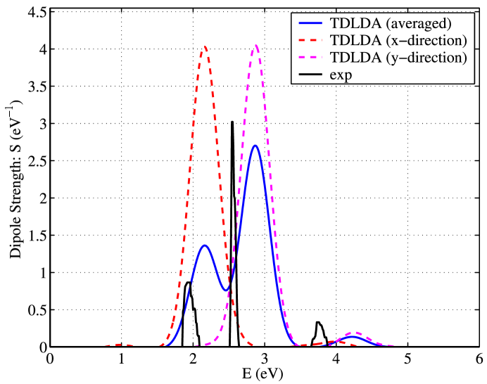
Figure 1: Optical absorption spectra of ${\rm Na}_{2}$ cluster obtained from direct time-stepping TDLDA calculation using norm-conserving TM pseudopotential. The results should be compared with Fig. 1 of Marques et al. Marques et al. (2001).

For the ${\rm Na}_{2}$ cluster, we actually use norm-conserving TM pseudopotential DAC (web site) for the Na atom, which is a special limiting case of our USPP-TDDFT code. The supercell is a tetragonal box of $12\times 10\times 10\;{\rm\AA}^{3}$ and the ${\rm Na}_{2}$ cluster is along the $x$-direction with a bond length of $3.0\;{\rm\AA}$. The planewave basis has a kinetic energy cutoff of $300$ eV. The time integration is carried out for $10,000$ steps with a timestep of $\Delta t=1.97$ attoseconds, and $\epsilon=0.01/{\rm\AA}$, $\gamma=0.02{\rm eV}^{2}/\hbar^{2}$. In the dipole strength plot (Fig. 1), the three peaks agree very well with TDLDA result from Octopus Marques et al. (2001), and differ by $\sim 0.4$ eV from the experimental peaks Sinha (1949); Fredrickson and Watson (1927). In this case, the $f$-sum rule is verified to be satisfied to within $0.1\%$ numerically.

For the benzene molecule, ultrasoft pseudopotentials are used for both carbon and hydrogen atoms. The calculation is performed in a tetragonal box of $12.94\times 10\times 7\;{\rm\AA}^{3}$ with the benzene molecule placed on the $x-y$ plane. The C-C bond length is $1.39\;{\rm\AA}$ and the C-H bond length is $1.1\;{\rm\AA}$. The kinetic energy cutoff is $250$ eV, $\epsilon=0.01/{\rm\AA}$, $\gamma=0.1{\rm eV}^{2}/\hbar^{2}$, and the time integration is carried out for $5000$ steps with a timestep of $\Delta t=2.37$ attoseconds. In the dipole strength function plot (Fig. 2), the peak at $6.95$ eV represents the $\pi\rightarrow\pi^{*}$ transition and the broad peak above $9$ eV corresponds to the $\sigma\rightarrow\sigma^{*}$ transition. The dipole strength function agrees very well with other TDLDA calculations Yabana and Bertsch (1999); Marques et al. (2003) and experiment Koch and Otto (1972). The slight difference is mostly due to our ad hoc approximation that ${\psi}_{n}$’s instead of $\tilde{\psi}_{n}$’s are used in (40). The more formally rigorous implementation of the electric impulse perturbation, Eq. (46), will be performed in future work.

Figure 2: Optical absorption spectrum of benzene (${\rm C}_{6}{\rm H}_{6}$) molecule. The results should be compared with Fig. 2 of Marques et al. Marques et al. (2003)

In this section we have verified the soundness of our time stepper with planewave basis through two examples of explicit electronic dynamics, where the charge density and effective potential are updated at every timestep, employing both norm-conserving and ultrasoft pseudopotentials. This validation is important for the following non-perturbative propagation of electrons in more complex systems.

V Fermi Electron Transmission

We first briefly review the setup of the Landauer transmission equation, Landauer (1957, 1970); Imry and Landauer (1999) before performing an explicit TDDFT simulation. In its simplest form, two identical metallic leads (see Fig. (3)) are connected to a device. The metallic lead is so narrow in $y$ and $z$ that only one channel (lowest quantum number in the $y,z$ quantum well) needs to be considered. In the language of band structure, this means that one and only one branch of the 1D band structure crosses the Fermi level $E_{\rm F}$ for $k_{x}>0$. Analogous to the universal density of states expression $dN=2\Omega dk_{x}dk_{y}dk_{z}/(2\pi)^{3}$ for 3D bulk metals, where $\Omega$ is the volume and the factor of $2$ accounts for up- and down-spins, the density of state of such 1D system is simply

$$dN\;=\;\frac{2Ldk_{x}}{2\pi}.$$ (47)

In other words, the number of electrons per unit length with wave vector $\in(k_{x},k_{x}+dk_{x})$ is just $dk_{x}/\pi$. These electrons move with group velocity Peierls (1955):

$$v_{\rm G}\;=\;\frac{dE(k_{x})}{\hbar dk_{x}},$$ (48)

so there are $(dk_{x}/\pi)(dE(k_{x})/(\hbar dk_{x}))=2dE/h$ such electrons hitting the device from either side per unit time.

Figure 3: Illustration of the Landauer transmission formalism.

Under a small bias voltage $dV$, the Fermi level of the left lead is raised to $E_{\rm F}+edV/2$, while that of the right lead drops to $E_{\rm F}-edV/2$. The number of electrons hitting the device from the left with wave vector $(k_{x},k_{x}+dk_{x})$ is exactly equal to the number of electrons hitting the device from the right with wave vector $(-k_{x},-k_{x}-dk_{x})$, except in the small energy window $(E_{\rm F}-edV/2,E_{\rm F}+edV/2)$, where the right has no electrons to balance against the left. Thus, a net number of $2(edV)/h$ electrons will attempt to cross from left and right, whose energies are very close to the original $E_{\rm F}$. Some of them are scattered back by the device, and only a fraction of $T\in(0,1]$ gets through. So the current they carry is:

$$\left.\frac{dI}{dV}\right|_{V=0}\;=\;\frac{2e^{2}}{h}T(E_{\rm F}),$$ (49)

where ${2e^{2}}/{h}=77.481\mu S=(12.906k\Omega)^{-1}$.

Clearly, if the device is also of the same material and structure as the metallic leads, then $T(E_{\rm F})$ should be $1$, when we ignore electron-electron and electron-phonon scattering. This can be used as a sanity check of the code. For a nontrivial device however such as a molecular junction, $T(E_{\rm F})$ would be smaller than $1$, and would sensitively depend on the alignment of the molecular levels and $E_{\rm F}$, as well as the overlap between these localized molecular states and the metallic states.

Here we report two USPP-TDDFT case studies along the line of the above discussion. One is an infinite defect-free gold chain (Fig. 4(a)). The other case uses gold chains as metallic leads and connects them to a -S-C₆H₄-S- (benzene-(1,4)-dithiolate, or BDT) molecular junction (Fig. 4(b)).

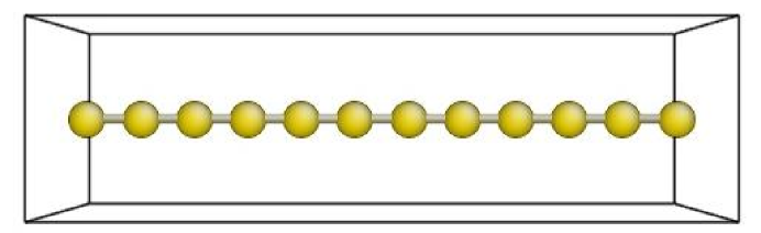
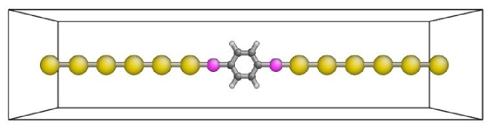
Figure 4: Atomistic configurations of our USPP-TDDFT simulations (Au: yellow, S: magenta, C: black, and H: white). (a) 12-atom Au chain. Bond length: Au-Au 2.88 $\;{\rm\AA}$. (b) BDT (-S-C₆H₄-S-) junction connected to Au chain contacts. Bond lengths: Au-Au 2.88 Å, Au-S 2.41 Å, S-C 1.83 Å, C-C 1.39 Å, and C-H 1.1 Å.

In the semi-classical Landauer picture explained above, the metallic electrons are represented by very wide Gaussian wavepacks Peierls (1955) moving along with the group velocity $v_{\rm G}$, and with negligible rate of broadening compare to $v_{\rm G}$. Due to limitation of computational cost, we can only simulate rather small systems. In our experience with 1D lithium and gold chains, a Gaussian envelop of 3-4 lattice constants in full width half maximum is sufficient to propagate at the Fermi velocity $v_{\rm G}(k_{\rm F})$ with 100% transmissions and maintain its Gaussian-profile envelop with little broadening for several femto-seconds.

V.1 Fermi electron propagation in gold chain

The ground-state electronic configurations of pure gold chains are calculated using the free USPP-DFT package DACAPO, DAC (web site); Hammer et al. (1999); Bahn and Jacobsen (2002) with local density functional (LDA) Ceperley and Alder (1980); Perdew and Zunger (1981) and planewave kinetic energy cutoff of $250$ eV. The ultrasoft pseudopotential is generated using the free package uspp (ver. 7.3.3) Vanderbilt (1990); Laasonen et al. (1991, 1993), with $5d$, $6s$, $6p$, and auxiliary channels. Fig. 4(a) shows a chain of 12 Au atoms in a tetragonal supercell ($34.56\times 12\times 12$ ų), with equal Au-Au bond length of $2.88$ Å. Theoretically, 1D metal is always unstable against period-doubling Peierls distortion Peierls (1955); Marder (2000). However, the magnitude of the Peierls distortion is so small in the Au chain that room-temperature thermal fluctuations will readily erase its effect. For simplicity, we constrain the metallic chain to maintain single periodicity. Only the $\Gamma$-point wavefunctions are considered for the 12-atom configuration.

The Fermi level $E_{\rm F}$ is found to be $-6.65$ eV, which is confirmed by a more accurate calculation of a one-Au-atom system with k-sampling (Fig. 5). The Fermi state is doubly degenerate due to the time-inversion symmetry, corresponding to two Bloch wavefunctions of opposite wave vectors $k_{\rm F}$ and $-k_{\rm F}$.

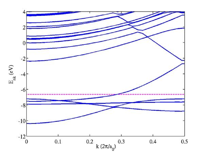
Figure 5: Band structure of a one-atom Au chain with 64 Monkhorst-PackMonkhorst and Pack (1976) k-sampling in the chain direction. The Fermi level, located at $-6.65$ eV, is marked as the dashed line.

From the $\Gamma$-point calculation, two energetically degenerate and real eigen-wavefunctions, $\psi_{+}({\bf x})$ and $\psi_{-}({\bf x})$, are obtained. The complex traveling wavefunction is reconstructed as

$$\psi_{k_{\rm F}}({\bf x})=\frac{\psi_{+}({\bf x})+i\psi_{-}({\bf x})}{\sqrt{2}}.$$ (50)

The phase velocity of ${\psi}_{k_{\rm F}}({\bf x},t)$ computed from our TDLDA runs matches the Fermi frequency $E_{\rm F}/\hbar$. We use the integration scheme (37) and a timestep of $2.37$ attoseconds.

We then calculate the Fermi electron group velocity $v_{\rm G}(k_{\rm F})$ by adding a perturbation modulation of

$$\widetilde{\psi}_{k_{\rm F}}({\bf x},t=0)\;=\;\psi_{k_{\rm F}}({\bf x})(1+\lambda\sin(2\pi x/L))$$ (51)

to the Fermi wavefunction ${\psi}_{k_{\rm F}}({\bf x})$, where $\lambda$ is $0.02$ and $L$ is the $x$-length of the supercell. Fig. 6 shows the electron density plot along two axes, $x$ and $t$. From the line connecting the red-lobe edges, one can estimate the Fermi electron group velocity to be $\sim$10.0 Å/fs. The Fermi group velocity can also be obtained analytically from Eq. (48) at $k_{x}=k_{\rm F}$. A value of 10 Å/fs is found according to Fig. 5, consistent with the TDLDA result.

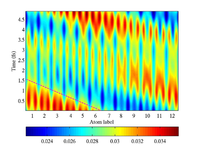
Figure 6: Evolution of modulated Fermi electron density in time along the chain direction. The electron density, in the unit of ${\rm\AA}^{-1}$, is an integral over the perpendicular $y$-$z$ plane and normalized along the $x$ direction, which is then color coded.

Lastly, the angular momentum projected densities of states are shown in Fig. 7, which indicate that the Fermi wavefunction mainly has $s$ and $p_{x}$ characteristics.

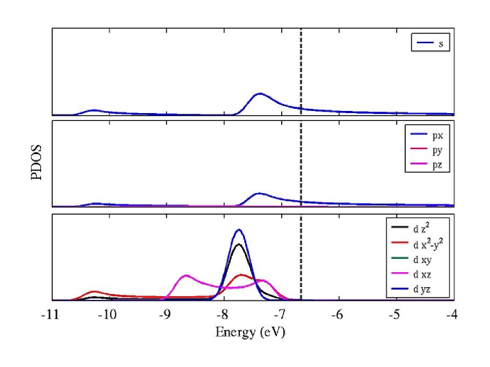
Figure 7: Projected density of states of the 12-atom Au chain.

V.2 Fermi electron transmission through Au-BDT-Au junction

At small bias voltages, the electric conductance of a molecular junction (Fig. 4(b)) is controlled by the transmission of Fermi electrons, as shown in Eq. (49). In this section, we start from the Fermi electron wavefunction of a perfect 1D gold chain (Fig. 4(a)), and apply a Gaussian window centered at ${\bf x}_{0}$ with a half width of $\sigma$, to obtain a localized wave pack

$$\widetilde{\psi}_{k_{\rm F}}({\bf x},t=0)={\psi}_{k_{\rm F}}({\bf x})G\left(\frac{{\bf x}-{\bf x}_{0}}{\sigma}\right),$$ (52)

at the left lead. This localized Fermi electron wave pack is then propagated in real time by the TDLDA-USPP algorithm (37) with a timestep of $2.37$ attoseconds, leaving from the left Au lead and traversing across the -S-C₆H₄-S- molecular junction (Fig. 4(b)). While crossing the junction the electron will be scattered, after which we collect the electron density entering the right Au lead to compute the transmission probability $T(E_{\rm F})$ literally. The calculation is performed in a tetragonal box ($42.94\times 12\times 12$ ų) with a kinetic energy cutoff of $250$ eV.

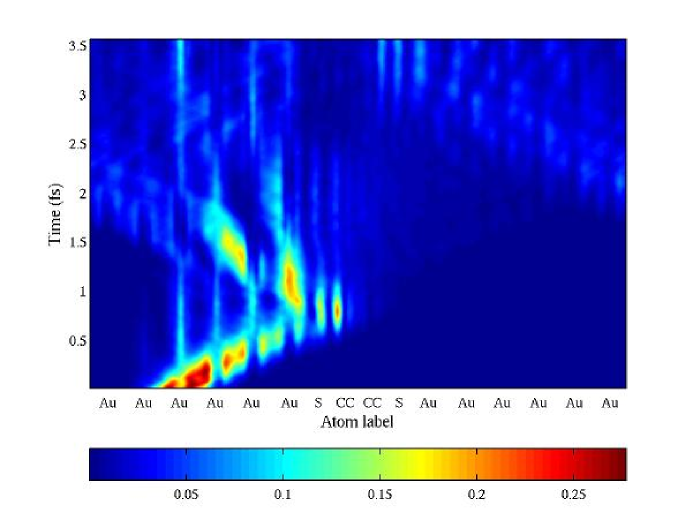
Figure 8: Evolution of filtered wave package density in time along the chain direction. The electron density, in the unit of ${\rm\AA}^{-1}$, is a sum over the perpendicular $y$-$z$ plane and normalized along the $x$ direction. The normalized electron density is color coded by the absolute value.

Fig. 8 shows the Fermi electron density evolution in $x$-$t$. A group velocity of $10$ Å/fs is obtained from the initial wave pack center trajectory, consistent with the perfect Au chain result. This free propagation lasts for about $0.8$ fs, followed by a sharp density turnover that indicates the occurrence of strong electron scattering at the junction. A very small portion of the wave pack goes through the molecule. After about $1.7$ fs, the reflected portion of the wave pack enters the right side of the supercell through PBC.

To separate the transmitted density from the reflected density as clearly as possible, we define and calculate the following cumulative charge on the right side

$$R(x^{\prime},t)\;\equiv\;\int_{x_{\rm S}}^{x^{\prime}}dx\int_{0}^{L_{y}}dy\int_{0}^{L_{z}}dz\rho(x,y,z,t),$$ (53)

where $x_{\rm S}$ is the position of the right sulfur atom. $R(x^{\prime},t)$ is plotted in Fig. 9 for ten $x^{\prime}$-positions starting from the right sulfur atom up to the right boundary $L_{x}$. A shoulder can be seen in all 10 curves, at $t=1.5$-$2$ fs, beyond which $R(x^{\prime},t)$ starts to rise sharply again, indicating that the reflected density has entered from the right boundary. Two solid curves are highlighted in Fig. 9. The lower curve is at $x^{\prime}=x_{\rm S}+7.2$ Å, which shows a clear transmission plateau of about $5$%. The upper curve, which is for $x^{\prime}$ exactly at the right PBC boundary, shows $R(x^{\prime},t)\approx 7$% at the shoulder. From these two curves, we estimate a transmission probability $T(E_{\rm F})$ of $5$-$7$%, which corresponds to a conductance of $4.0$-$5.6$ $\mu$S according to Eq. (49). This result from planewave TDLDA-USPP calculation is comparable to the transmission probability estimate of $10$% from complex band structure calculation Tomfohr and Sankey (2002a, b) for one benzene linker (-C₆H₄-) without the sulfur atoms, and the non-equilibrium Green’s function estimate of $5$ $\mu$S Xue and Ratner (2003) for the similar system.

Figure 9: $R(x^{\prime},t)$ versus time plot. Curves are measured in $10$ different regions with different $x^{\prime}$ positions, which equally divide the region from the right S atom to the boundary on the right hand side.

VI Summary

In this work, we develop TDDFT based on Vanderbilt ultrasoft pseudopotentials and benchmark this USPP-TDDFT scheme by calculating optical absorption spectra, which agree with both experiments and other TDDFT calculations. We also demonstrate a new approach to compute the electron conductance through single-molecule junction via wave pack propagation using TDDFT. The small conductance of $4.0$-$5.6$ $\mu$S is a result of our fixed band approximation, assuming the electron added was a small testing electron and therefore generated little disturbing effects of the incoming electrons on the electronic structure of the junction. This result is of the same order of magnitude as the results given by the Green’s function and the complex band approaches, both requiring similar assumptions.