Robust Emergent Activity in Dynamical Networks

Abstract

We study the evolution of a random weighted network with complex nonlinear dynamics at each node, whose activity may cease as a result of interactions with other nodes. Starting from a knowledge of the micro-level behaviour at each node, we develop a macroscopic description of the system in terms of the statistical features of the subnetwork of active nodes. We find the asymptotic characteristics of this subnetwork to be remarkably robust: the size of the active set is independent of the total number of nodes in the network, and the average degree of the active nodes is independent of both the network size and its connectivity. These results suggest that very different networks evolve to active subnetworks with the same characteristic features. This has strong implications for dynamical networks observed in the natural world, notably the existence of a characteristic range of links per species across ecological systems.

With the recent surge of interest in complex networks Newman , the behaviour of dynamical units interacting on networks has become a problem of crucial relevance to areas ranging from physics to biology to engineering. Coupled nonlinear systems, such as oscillators and maps, have been extensively investigated on regular lattices Kan . The graph theoretic aspects of random networks have also received considerable attention Bollobas . However, there have been very few studies on networks with nonlinear dynamics at the nodes. Here we focus on this relatively unexplored area of random networks of nonlinear maps, and study the role played by the network properties on the time-evolution of the dynamical states of the nodes, in particular, and the global characteristics of the evolved network, in general.

We consider networks with a wide range of ($i$) size (i.e., number of nodes, $N$), ($ii$) connectivity $C$ between nodes (i.e., the density of links), ($iii$) measure of interaction strength $\sigma$ that determines the weights of the connections (i.e., how strongly the nodes are coupled) and ($iv$) local dynamics at the nodes (ranging from regular to chaotic). The important feature here is that even though the isolated nodes may exhibit a wide range of activity, the network yields generically chaotic global dynamics. This can result in a fraction of the nodes being driven to a state of null activity, implying that under interactions a certain set of nodes show a transition from persistent to transient activity. In this paper, we examine the properties of the subnetwork of nodes with persistent activity. We show that the size of this subnetwork of active nodes is remarkably independent of the network size. Further, the total number of links in this subnetwork is independent of both the size and the connectivity of the network. These results have considerable significance for the observable properties of networks occurring in nature.

The work reported in this paper can be seen in the context of deriving a statistical mechanics of interacting dynamical elements Ker57 ; Lei65 . Starting from a micro-level dynamical description, where the relevant variables are the local states of each node in the network, we would like to achieve a macroscopic description of the system in terms of the number of active nodes, and would like to understand how such macro-variables are determined by overall network properties, such as, $N$, $C$ and $\sigma$. One would have naively supposed that the macroscopic system variable of interest, namely, the size of the persistently active subnetwork, would be an extensive quantity. However, our results show that this macroscopic quantity does not scale with system size. This implies the existence of “universal” relations between various gross network properties in the asymptotic state, and the emergence of characteristic robust features independent of network size.

Our model is quite general: it has $N$ dynamical elements in a network with random nonlocal connectivity. The dynamical state of each node $i(=1\ldots N)$ at time $n$ is associated with a continuous variable $x_{i}(n)$, which is the microscopic variable of interest in the system. The interaction between two nodes is given by a coupling coefficient $J_{ij}$. We consider the most general case where these coefficients can be asymmetric ($J_{ij}\neq J_{ji}$) and can be either positive or negative. The time-evolution of the system is given by

$$x_{i}(n+1)=f[x_{i}(n)\{1+\Sigma_{j}J_{ij}x_{j}(n)\}],$$ (1)

where $f$ represents the local on-site dynamics. In this paper we have shown representative results for $f$ chosen to be the exponential map,

$$f(x)=xe^{r(1-x)},~{}{\rm if}~{}x>0;~{}=0,~{}{\rm otherwise},$$ (2)

$r$ being the nonlinearity parameter leading from periodic behaviour to chaos Ric54 . This belongs to the class of maps defined over the semi-infinite interval $[0,\infty]$ rather than a finite, bounded interval (e.g., as is the case for logistic map). This allows us to explore arbitrary distributions of couplings between nodes, unlike maps bounded in an interval, which are well-behaved only for restrictive coupling schemes. In addition, in our case, the nonlinearity parameter $r$ is not artificially restricted by the domain of definition of the map. All these features increase the generality of our results, and additionally, such maps provide a more accurate description of natural processes, e.g., population dynamics Has76 ; Bel81 .

The connectivity matrix ${\bf J}=\{J_{ij}\}$ is, in general, a sparse matrix, with probability $1-C$ that an element is zero. The diagonal entries $J_{ii}=0$ indicate that in the absence of interactions, the local nonlinear map (2) completely determines the dynamical state of each node. The non-zero entries in the matrix are chosen from a normal distribution with mean 0 and variance $\sigma^{2}$. Note that we have also used uniform distributions over the interval $[-\sigma,\sigma]$ without any qualitative changes in the results.

Initially, the states of all the $N$ nodes are randomly distributed about $x=1$. During the evolution of the network, if the state of a node becomes $x\leq 0$, it stops being active and subsequently has no interaction with the rest of the network. Note that, in the absence of coupling, the maps describing the dynamics at individual nodes do not cease activity. This allows us to focus on the instability induced by network interactions, rather than the intrinsic behaviour of the nodes. As a result of these interactions, the number of persistent nodes (i.e., with $x>0$) decreases rapidly from the initial value, but eventually attains a steady state. This is because, at the initial stages, the population of each node undergoes strong fluctuations due to interaction with other nodes coupled to it, resulting in the cessation of activity of a large number of nodes. Within a very short time, the effective number of interacting nodes decrease and, consequently, the intensity of such fluctuations is also reduced. We have continued the simulations for up to $10^{4}$ iterations, when the probability of further extinctions was found to become extremely small. We then look at the number of nodes which survive with persistent activity as a function of the model parameters (Fig. 1).

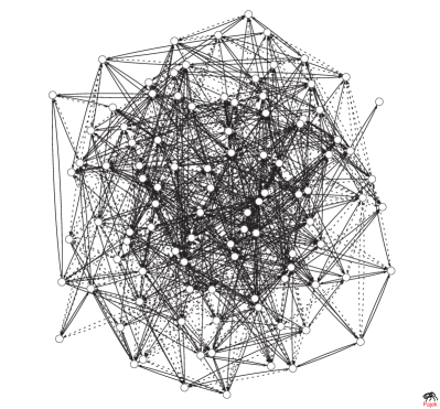
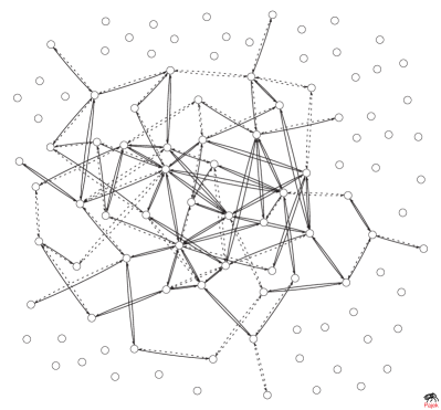
Figure 1: The initial (left) and asymptotic (right) state of a network with $N=100$, $C=0.1$, $\sigma=0.1$, $r=4$. Only the connections between active nodes are shown. Solid lines represent positive links, while broken lines represent negative links.

The number of nodes with persistent activity is a measure of the global stability of the network. The information that we get from this is very different from the local stability and complementary to it. Note that, in the study of interdisciplinary problems, global stability (or persistence) is often much more relevant than the more commonly used measures of local stability. For example, networks susceptible to catastrophic failures or crashes are extremely common in the real world. In such problems, the quantity of interest is the system’s global stability, as reflected in the survival probability of nodal activity, rather than local stability, which, in the absence of regular equilibria, does not contribute to our understanding of the overall system dynamics note1 .

We now look at the features of the asymptotic subnetwork consisting of the nodes which survive with persistent activity. The first significant feature of this emergent subnetwork is that its size is independent of the system size $N$. This is clearly evident from Fig. 2, which shows that the size of the active subnetwork quickly approaches its asymptotic value $N_{active}$ which is a constant with respect to $N$ (within error bars). For example, for the representative case of $\sigma=0.1,C=1,r=4$, we find that $N_{active}=7.705\pm 1.260$ for $N=250$, while for $N=1000$, $N_{active}=7.835\pm 1.247$.

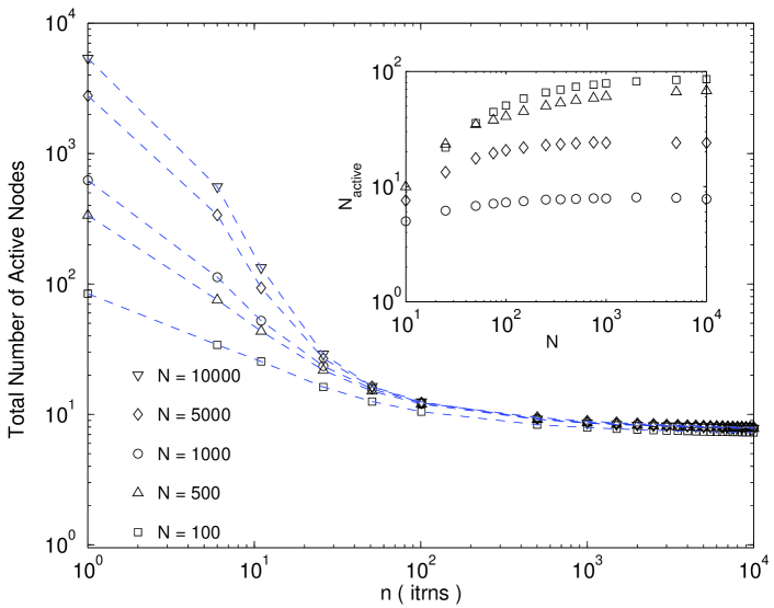
Figure 2: Time-evolution of the number of active nodes for networks of various sizes $N$ ($C$ = 1, $\sigma$ = 0.1 , $r=4$), showing the rapid decay to the asymptotic value that is independent of $N$. (Inset) The asymptotic number of active nodes, $N_{active}$, as a function of network size $N$ ($\square$: $C$ = 0.1, $\sigma$ = 0.1, $r=4$; $\bigtriangleup$: $C$ = 1, $\sigma$ = 0.1, $r=2$; $\diamond$: $C$ = 0.1, $\sigma$ = 0.5, $r=4$; $\circ$: $C$ = 1, $\sigma$ = 0.1, $r=4$). Note that, in all cases, $N_{active}$ is independent of the network size $N$, for large $N$.

In the absence of connections ($C=0$), $N_{active}$ ($=N$) is obviously extensive. But for $C>0$, $N_{active}$ saturates to a value independent of $N$. This non-extensivity for the active subnetwork has significant implications. For instance, let us consider two stable networks, each of which has $N_{active}$ persistently active nodes. On being joined together (analogous to two distinct ecological systems being suddenly linked to one another), the merger initially results in a high number of active nodes, which is essentially the sum of the active nodes of the two components (= $2N_{active}$). However, the new connections prompt a fresh wave of extinctions to occur, resulting in the number of active nodes rapidly settling back to the characteristic value $N_{active}$.

Another remarkable feature is that the average number of links per node in the active subnetwork, $k_{active}$, is independent of $N$, as well as $C$. Therefore, $k_{active}$ is independent of $k_{0}(=NC)$, the average degree of the entire network (Fig. 3). The significance of this result is evident: regardless of the size and connectivity of the network, the nodes in the active subnetwork has a characteristic number of links. Together with the earlier result of a characteristic size for the active subnetwork ($N_{active}$), this implies that the total number of links ($N_{active}\times k_{active}$) connecting the active nodes is a robust quantity.

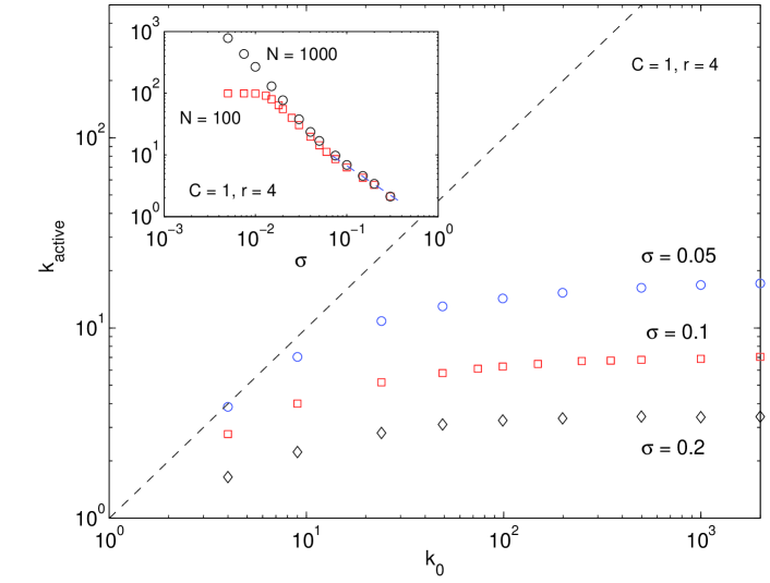
Figure 3: Asymptotic number of links per node in the active subnetwork ($k_{active}$) as a function of the number of links per node of the full network ($k_{0}$) for different values of $\sigma$ ($C=1,r=4$). The broken line represents $k_{active}=k_{0}$. The inset shows $k_{active}$ as a function of $\sigma$ for $N=100$ and 1000. Note that the two data sets converge at a high value of $\sigma$ and match well with the broken line representing $\sim 1/\sigma$.

The active subnetwork is further characterised by disassortativity, i.e., nodes with high degree connect preferentially to nodes having fewer links, a feature observed in many biological and technological networks. For instance, the disassortativity index as defined by Newman New02 is $-0.11$ for $N=100,C=0.5,\sigma=0.1,r=4$.

The fact that the size of the active set is independent of the network size $N$ may be naively expected from the May-Wigner stability criterion Sin05 . According to this, a system is critically stable if $NC\sigma^{2}\simeq 1$. So the size of the asymptotically stable set $N_{active}$ is proportional to $1/C\sigma^{2}$. However, note that, in an evolving system, the values of $C$ and $\sigma$ for the active set also change significantly over time, with nodes becoming inactive and their links becoming non-functional. As a result, we have an interplay between the size and structure of the subnetwork of active nodes: the size of this set changes due to the stability criterion involving the structural parameters $C$ and $\sigma$ at that point in time, while the latter ($C$, $\sigma$) themselves change due to the reduction in the number of active nodes. For the May-Wigner argument to hold, it is crucial that $C$ and $\sigma$ eventually attain their own asymptotic values $C_{active}$ and $\sigma_{active}$, and that these are independent of network size $N$. To verify this we now look at these properties in the asymptotic set of active nodes.

Figure 4: The persistence probability (i.e., survival of activity) of individual nodes as a function of the fraction of negative links to that node, appropriately scaled by the network size $N$, so that data for different values of $N$ ($\bigtriangleup$: $N=250$, $\circ$: $N=100$, $\times$: $N=50$) collapse on the same curve using $F_{c}^{N}=0.1$ for $N=50$, $=0.06$ for $N=100$ and $=0.039$ for $N=250$. The network parameters are $C=0.1$, $\sigma=0.1$ and $r=4$. The inset shows the connectivity of the active subnetwork, $C_{active}$, as a function of $C$ for two different network sizes.

First, we examine how the effective connectivities of the asymptotic subnetwork, $C_{active}$, is different from the network connectivity, $C$. Remarkably, $C_{active}$ is found to be independent of the network size for large $N$. For $0<C<1$, the effective connectivity of the asymptotic subnetwork shows a clear trend of evolving to a slightly lower value compared to $C$ [Fig. 4 (inset)], with the deviation increasing with average interaction strength, $\sigma$ and local nonlinearity parameter, $r$. The independence of $C_{active}$ from $N$ can also be inferred from Fig. 3, by noting that the $k_{active}$ vs $k_{0}$ curve can be constructed entirely by considering $C=1$, for which $C_{active}(=C)$ is obviously independent of $N$. The same curve holds for other values of $C$ and therefore one can conclude that $C_{active}$ is independent of $N$, for all $C$. Further, $N_{active}\sim 1/C_{active}$ Sin05 , which is consistent with our earlier result that $N_{active}$ is independent of $N$.

Next, we address the question of the independence of $\sigma_{active}$ with respect to $N$, by looking at the distribution of the connection weights $J_{ij}$ of the persistent nodes. Specifically, we examine how this differs from the distribution of $J_{ij}$ in the full network. We observe that starting from a Gaussian distribution (for instance), the distribution that emerges is independent of $N$, indicating that $\sigma_{active}$ is independent of the network size. Further, the distribution is markedly skewed towards positive weights implying a selective tendency of nodes with high negative links to be eliminated. This is consistent with the probability of survival of a single node being a decreasing function of the relative number of its negative links (Fig. 4).

Figure 5: Distribution of the (non-zero) interaction strengths $J_{ij}$ between active nodes of a network for $C=0.5,\sigma=0.1$ (solid line), $C=1,\sigma=0.1$ (dashed line) and $C=0.5,\sigma=0.2$ (dotted line). Note that, the cutoff at the lower end, $J^{*}$, is independent of $\sigma$. The inset shows the $J_{ij}$ distribution in the full network for the same set of parameters.

To explain the numerical results that show the average degree of the active subnetwork, $k_{active}$, evolving to a characteristic value, we recall that the average number of links per node is given by the product of $N_{active}$ and $C_{active}$. The $C_{active}$ does not vary too much from $C$, but $N_{active}$ varies significantly from $N$. So, the number of links essentially is dependent only on $N_{active}$. If $N_{active}$ settles down to the same constant value independent of $N$, it implies that the number of links is also a robust quantity (Fig. 3).

Further, $k_{active}$ varies with the overall network average interaction strength as $\sim 1/\sigma$ [Fig. 3 (inset)]. This can be understood from the condition determining persistence of activity for an individual node $i$: $P(\sum_{j}J_{ij}x_{j}<-1)$. Note that, the contributing terms in the sum are due to active nodes which have outgoing links (with non-zero weights) to node $i$, i.e., the degree of the node in the active subnetwork. From Fig. 5, it is apparent that the asymptotic distribution of $J_{ij}$ for the set of active nodes has a positive mean, $\mu$. This implies that the quantity $\sum_{j}J_{ij}x_{j}$ has a standard deviation, which is dominated by the leading term, $\mu k_{active}$, implying $k_{active}\sim 1/\mu$. To see how $\mu$ is related to $\sigma$, we look in detail at the asymptotic distribution of $J_{ij}$. It is immediately apparent that the dominant change in the asymptotic distribution, vis-a-vis the original distribution is the loss of the strong negative links. This results in the final distribution being truncated at the negative end, with the cutoff $J^{*}$ apparently independent of $\sigma$ (Fig. 5). Assuming that the positive part of the distribution is almost unchanged from its original form, we see that $\mu=\int_{J^{*}}^{\infty}J_{ij}P(J_{ij})$ essentially goes as $\sigma$, as the shift of the mean from zero is entirely determined by the width of the original distribution.

In conclusion, we have shown that a very simple model, with very few assumptions regarding the node properties and their dynamics, yields surprisingly robust macroscopic features of the emergent active system: (a) the asymptotic number of active nodes is independent of the network size, and (b) the asymptotic number of links between the active nodes is independent of both the size of the network and its connectivity. The link removal process is not guided here by any explicit criterion designed to achieve a desired end-state but emerges naturally from the dynamics at the nodes.

The observed non-extensivity of the active subnetwork indicates that designing robust structures simply by increasing the redundancy of nodes, keeping the connectivity and interaction strength distribution unchanged, is not a good strategy, as the number of asymptotically active nodes is independent of the initial number of nodes that one starts out with. This provides an explanation for similar observations in natural and artificial complex systems, such as the conservation of the number of species in an ecosystem after major extinctions (e.g., after the eruption in Krakatoa) or migrations (e.g., after the linking of North and South America) May78 , as well as the existence of a characteristic range of links per species (3 to 5) across different environments May88 .

References

- (1) M. E. J. Newman, SIAM Rev. 45, 167 (2003).
- (2) K. Kaneko (Ed.) Theory and Applications of Coupled Map Lattices, (John Wiley, New York, 1993).
- (3) B. Bollobas Random Graphs, (Academic Press, London, 1985).
- (4) E. H. Kerner, Bull. Math. Biophys. 19, 121 (1957).
- (5) E. G. Leigh, Proc. Natl. Acad. Sci. (USA) 53, 777 (1965).
- (6) W. E. Ricker, J. Fish. Res. Board Can. 11, 559 (1954).
- (7) M. P. Hassell, J. H. Lawton and R. M. May, J. Anim. Ecol. 45, 471 (1976).
- (8) T. S. Bellows, J. Anim. Ecol. 50, 139 (1981).
- (9) We would like to point out that the dynamics of the asymptotic network does not lead to a fully, or even, partially synchronised state between the nodes. Indeed there is no global equilibrium, which is verified by calculating the spectrum of lyapunov exponents of the system. The spectrum shows strong spatiotemporal chaos in the global dynamics with no apparent synchronisation between the nodes with persistent activity. Even when the local dynamics is regular, the global dynamics of the coupled system does show chaos.
- (10) M. E. J. Newman, Phys. Rev. Lett. 89, 208701 (2002).
- (11) S. Sinha and S. Sinha, Phys. Rev. E 71, 020902 (2005).
- (12) R. M. May, Sci. Am. 239(3), 161 (1978).
- (13) R. M. May, Science 241, 1441 (1988).