Exact solution of $Z_{2}$ Chern-Simons model on a triangular lattice

Abstract

We construct the Hamiltonian description of the Chern-Simons theory with $Z_{n}$ gauge group on a triangular lattice. We show that the $Z_{2}$ model can be mapped onto free Majorana fermions and compute the excitation spectrum. In the bulk the spectrum turns out to be gapless but acquires a gap if a magnetic term is added to the Hamiltonian. On a lattice edge one gets additional non-gauge invariant (matter) gapless degrees of freedom whose number grows linearly with the edge length. Therefore, a small hole in the lattice plays the role of a charged particle characterized by a non-trivial projective representation of the gauge group, while a long edge provides a decoherence mechanism for the fluxes. We discuss briefly the implications for the implementations of protected qubits.

I Introduction.

The challenge of the error free quantum computation Kitaev2002 ; Childs2002 ; Preskill1998 resulted in a surge of interest to many physical systems and mathematical models that were considered very exotic before. While it is clearly very difficult (if not impossible) to satisfy the conditions of long decoherence rate and scalability in simple physical systemsIoffe2004 , both can be in principle satisfied if elementary bits are represented by anyons, the particles that indergo non-trivial transformations when moved adiabatically around each other (braided) Kitaev1997 ; Mochon2003 ; Mochon2004 . One of the most famous examples of such excitations is provided by the fractional Quantum Hall Effect Halperin84 ; Arovas84 . The difficult part is, of course, to identify a realistic physical system that has such excitations and allows their manipulations. This problem should be separated into different layers. The bottom layer is the physical system itself, the second is the theoretical model that identifies the low energy processes, the third is the mathematical model that starts with the most relevant low energy degrees of freedom and gives the properties of anyons while the fourth deals with construction of the set of rules on how to move the anyons in order to achieve a set of universal quantum gates (further lies the layer of algorithms and so on).

One of the most interesting set of problems of the third layer is provided by the Chern-Simons theories with discrete groups on the lattice: on one hand in these theories one expects to have a non-local interaction between fluxes that gives them the anyonic properties, on the other hand they might describe physics of some solid state arrays. In particular, we have shown very recently Doucot2005 that ${\mathchoice{\hbox{$\sf\textstyle Z\kern-3.99994ptZ$}}{\hbox{$\sf\textstyle Z\kern-3.99994ptZ$}}{\hbox{$\sf\scriptstyle Z\kern-2.10002ptZ$}}{\hbox{$\sf\scriptscriptstyle Z\kern-0.99998ptZ$}}}_{2}$ Chern-Simons theory can be realistically implemented in a Josephson junction array on a square lattice. Furthermore, the ground state of these physical systems is doubly degenerate but locally instinguishable so that even a small sized lattice provides a very good protection of this degeneracy against the external noise. Such protection is expected to become ideal for the larger lattice sizes if the gap to excitations is finite. The lack of the exact solution did not allow us to make definite conclusions on the properties of this model for larger lattice sizes. However, the analytical solution in limiting cases combined with the extensive numerics Dorier2005 indicates that the gap for the low energy excitations closes in the thermodynamic limit. Practically, this would imply that protection that can be achieved in such arrays does not grow with the array size beyond a certain limit. In order to get a better understanding of the properties of such models we consider here a similar (${\mathchoice{\hbox{$\sf\textstyle Z\kern-3.99994ptZ$}}{\hbox{$\sf\textstyle Z\kern-3.99994ptZ$}}{\hbox{$\sf\scriptstyle Z\kern-2.10002ptZ$}}{\hbox{$\sf\scriptscriptstyle Z\kern-0.99998ptZ$}}}_{n}$ Chern-Simons) model on a triangular lattice. It turns out that for $n=2$ the model can be solved exactly by a mapping to Majorana fermions; we find the gapless spectrum of the photons which acquires a gap if additional (’magnetic’) terms are included in the Hamiltonian. We hope that long wave properties of this model are analogous to the properties of the square lattice model and thus the problem of the low energy excitations of the latter can be remedied by the ’magnetic’ field term in the Hamiltonian that plays the role of a tunable chemical potential for fluxes. Because it is difficult to avoid boundaries in a physical implementations, it is important to understand what is the effect of edges on the Chern-Simons theory. In particular, from the view point of the topological protection, it is important to understand whether they lead to gapless excitations such as edge states in Quantum Hall Effect.

Generally, while the lattice gauge theories without Chern-Simons term are well studied and understood, much less is known about their Chern-Simons counterparts. The reason for this is that Chern-Simons term implies coupling of the charge and flux; on a lattice the charge resides on the sites while the flux is associated with the plaquettes. Furthermore, one usually wants to preserve the symmetry of the lattice. To satisfy these criteria one has to couple charge with the total flux of a few adjacent plaquettes which leads to novel features absent in the continuous theories. We discuss the details of this construction in Section II. In particular, for a continuous Abelian gauge group the Chern-Simons term remains quadratic but becomes non-local in space, i.e. its Fourier transform acquires momentum dependence; moreover it is zero for some values of the momenta in the Brillouin zone. This leads to the appearance of the gapless modes in these theories in the absence of magnetic energy. Our analysis presented in Section III of the exactly solvable Chern-Simons theory with ${\mathchoice{\hbox{$\sf\textstyle Z\kern-3.99994ptZ$}}{\hbox{$\sf\textstyle Z\kern-3.99994ptZ$}}{\hbox{$\sf\scriptstyle Z\kern-2.10002ptZ$}}{\hbox{$\sf\scriptscriptstyle Z\kern-0.99998ptZ$}}}_{2}$ group shows that this qualitative picture holds for the discrete group as well. Finally, in Section IV we study the boundary effects and find that they are also similar for continuous and discrete groups. Namely, for continuous groups, the general arguments show Witten89 the appearance of a non-gauge invariant matter field on the boundary in Chern-Simons theories, similarly the exact solution of ${\mathchoice{\hbox{$\sf\textstyle Z\kern-3.99994ptZ$}}{\hbox{$\sf\textstyle Z\kern-3.99994ptZ$}}{\hbox{$\sf\scriptstyle Z\kern-2.10002ptZ$}}{\hbox{$\sf\scriptscriptstyle Z\kern-0.99998ptZ$}}}_{2}$ model shows that the same phenomena happens in discrete models as well.

II Model with ${\mathchoice{\hbox{$\sf\textstyle Z\kern-3.99994ptZ$}}{\hbox{$\sf\textstyle Z\kern-3.99994ptZ$}}{\hbox{$\sf\scriptstyle Z\kern-2.10002ptZ$}}{\hbox{$\sf\scriptscriptstyle Z\kern-0.99998ptZ$}}}_{n}$ symmetry

Let us first begin to discuss the construction of the Chern-Simons model with ${\mathchoice{\hbox{$\sf\textstyle Z\kern-3.99994ptZ$}}{\hbox{$\sf\textstyle Z\kern-3.99994ptZ$}}{\hbox{$\sf\scriptstyle Z\kern-2.10002ptZ$}}{\hbox{$\sf\scriptscriptstyle Z\kern-0.99998ptZ$}}}_{n}$ symmetry on the triangular lattice. The main element of this construction are the expressions for the electric field operators, $\mathcal{E}_{kl}^{\pm}$ and the local field translation operators $\mathcal{T}_{kl}^{\pm}$.Doucot2005 Both should preserve the symmetry of the lattice; furthermore, the expression for the electric field operators, $\mathcal{E}_{kl}^{\pm}$  should be gauge invariant while those for $\mathcal{T}_{kl}^{\pm}$ should preserve the electric fields operators. By analogy with our previous discussion for the square lattice Doucot2005 , we write:

$$\mathcal{E}_{kl}^{\pm} =\exp\left(\mp i\frac{2\pi}{n}\left(\Pi_{kl}-\sum_{(mn)}\nu(kl;mn)A_{mn}\right)\right)$$

$$\mathcal{T}_{kl}^{\pm} =\exp\left(\mp i\frac{2\pi}{n}\left(\Pi_{kl}+\sum_{(mn)}\nu(kl;mn)A_{mn}\right)\right)$$

Here $A_{kl}$ and $\Pi_{mn}$ are (discrete) gauge potential and canonical conjugate momentum on lattice link that satisfy usual canonical commutation relations:

$$[A_{kl},\Pi_{mn}]=i\delta_{(kl),(mn)}$$

where $(kl)$ and $(mn)$ denote oriented links on the triangular lattice. Reversing the orientation of a link changes the sign of the corresponding variables $A$ and $\Pi$. In the case of a ${\mathchoice{\hbox{$\sf\textstyle Z\kern-3.99994ptZ$}}{\hbox{$\sf\textstyle Z\kern-3.99994ptZ$}}{\hbox{$\sf\scriptstyle Z\kern-2.10002ptZ$}}{\hbox{$\sf\scriptscriptstyle Z\kern-0.99998ptZ$}}}_{n}$ symmetry, the local vector potentials $A_{kl}$ are constrained to be integer multiples of $2\pi/n$. The Chern-Simons coefficient $\nu(kl;mn)$ is zero unless $(mn)$ is one of the four neighbor links of $(kl)$ as illustrated on Fig. 1. In this case, $\nu(kl;mn)=\nu$, if the link $(mn)$ is oriented from right to left for an observer standing on link (kl) and looking towards site $l$. For the converse relative orientation, $\nu(kl;mn)=-\nu$

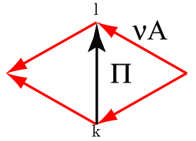
Figure 1: (Color online) The orientation convention used in the construction of a Chern-Simons model on a triangular lattice. The thick (black) line represents a $\Pi_{kl}$ operator, conjugated to the vector potential attached to the link. The arrow is required since $\Pi_{kl}=-\Pi_{lk}$. The gray (red) lines keep track of signs of $\nu(kl;lm)$ coefficients which appear in the phase-factors imposed by the Chern-Simons term in the definition of local electric operators $\mathcal{E}_{kl}^{\pm}$ and field translation operators $\mathcal{T}_{kl}^{\pm}$. Gray (red) lines are oriented from site $m$ to site $n$ whenever the coefficient $\nu(kl;mn)$ is positive.

The main consequence of these definitions is that the commutation relations of electric field operators on nearby links are modified by phase factors. For $(kl)$ and $(mn)$ oriented as on Fig. 1, we have:

$$\mathcal{E}_{kl}^{+}\mathcal{E}_{mn}^{+}=\exp\left(i(\frac{2\pi}{n})^{2}2\nu\right)\mathcal{E}_{mn}^{+}\mathcal{E}_{kl}^{+}$$ (1)

Similarly, the local field translation operators satisfy:

$$\mathcal{T}_{kl}^{+}\mathcal{T}_{mn}^{+}=\exp\left(-i(\frac{2\pi}{n})^{2}2\nu\right)\mathcal{T}_{mn}^{+}\mathcal{T}_{kl}^{+}$$ (2)

We shall focuss here on the case where these phase factors are equal to $-1$. This requires $\nu$ to be of the form:

$$\nu=\pi(\frac{n}{2\pi})^{2}(m+\frac{1}{2})$$ (3)

where $m$ is an integer.

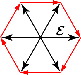
Figure 2: (Color online) Construction of the local gauge transformation generator based at the central site, see Eq. (5). Thick full links correspond to electric field operators $\mathcal{E}_{kl}^{+}$, and grey (red) oriented links to phase factors, $\exp(i\frac{8\pi\nu}{n}A_{mn})$, whose total contribution is equal to $\exp(-i\frac{8\pi\nu}{n}\Phi_{k})$, where $\Phi_{k}$ is the total flux (counted counterclockwise) through the hexagon.

To construct the ${\mathchoice{\hbox{$\sf\textstyle Z\kern-3.99994ptZ$}}{\hbox{$\sf\textstyle Z\kern-3.99994ptZ$}}{\hbox{$\sf\scriptstyle Z\kern-2.10002ptZ$}}{\hbox{$\sf\scriptscriptstyle Z\kern-0.99998ptZ$}}}_{n}$ model, we start from the system where local vector potentials can be arbitrary (and in particular unbounded) integer multiples of $2\pi/n$, and keep then only the subspace of periodic states $|\Psi\rangle$ which satisfy:

$$(\mathcal{T}_{kl}^{+})^{n}|\Psi\rangle=|\Psi\rangle$$ (4)

In general, this condition is not compatible with the possibility to perform arbitrary local gauge transformations, because the $\mathcal{T}_{kl}^{+}$ no longer commute with generators of local gauge transformations $U_{k}$ defined as:

$$U_{k}=\prod_{l}^{(k)}\mathcal{T}_{kl}^{+}=\prod_{l}^{(k)}\mathcal{E}_{kl}^{+}\exp(-i\frac{2\pi}{n}4\nu\Phi_{k})$$ (5)

where $\Phi_{k}=\sum_{hex}A_{mn}$ is the total flux through the loop composed by the six first neighbors of site $k$ and oriented counterclockwise, as illustrated on Fig. 2. This is an integer multiple of $2\pi/n$. Note that some care is required in chosing the order of the six operators involved in the above products. A convenient choice is to lump together each link $(kl)$ with its opposite $(kl^{\prime})$. This convention is sufficient to specify the total phase factor because $\mathcal{T}_{kl}^{+}$ operators on all but adjacent links commute (so that $[\mathcal{T}_{kl}^{+},\mathcal{T}_{kl^{\prime}}^{+}]=0$) while different pairs $\mathcal{T}_{kl}^{+}\mathcal{T}_{kl^{\prime}}^{+}$ commute because of the cancellation of the phase factors for any value of $\nu$. So, this choice yields three pairwise products which commute among themselves. With the notations of Fig. 2, we have:

$$U_{k}\mathcal{T}_{mn}=\exp\left(-i(\frac{2\pi}{n})^{2}4\nu\right)\mathcal{T}_{mn}U_{k}$$ (6)

Therefore, the ${\mathchoice{\hbox{$\sf\textstyle Z\kern-3.99994ptZ$}}{\hbox{$\sf\textstyle Z\kern-3.99994ptZ$}}{\hbox{$\sf\scriptstyle Z\kern-2.10002ptZ$}}{\hbox{$\sf\scriptscriptstyle Z\kern-0.99998ptZ$}}}_{n}$ periodicity conditions are compatible with local gauge invariance provided the quantity $(2\pi/n)^{2}4\nu n$ is an integer multiple of $2\pi$, which is clearly the case for $\nu$ chosen according to Eq. (3). Another important consequence of this choice is the very simple connection between generators of gauge transformations and local electric fields:

$$U_{k}=\prod_{l}^{(k)}\mathcal{E}_{kl}^{+}$$ (7)

A last consequence is that for any even value of $n$:

$$(\mathcal{E}_{kl}^{+})^{n}=(\mathcal{T}_{kl}^{+})^{n}$$ (8)

Once this set of basic operators has been defined, the natural gauge-invariant Hamiltonian is constructed as a sum of two terms: the first one involves local electric field operators on individual links and the second one the local magnetic fluxes around plaquettes. Specifically:

$$H=-\frac{1}{2}\sum_{(k,l)}(\mathcal{E}_{kl}^{+}+\mathcal{E}_{kl}^{-})+\sum_{(j,k,l)}f(\Phi(j,k,l))$$ (9)

The first sum is over links $(k,l)$ and the second one over elementary triangular plaquettes $(j,k,l)$ which are oriented counterclockwise. At this stage, $f$ may be any function and the flux $\Phi(j,k,l)=A_{ij}+A_{jk}+A_{kl}$. Note that we are not dealing here with the pure Chern-Simons theory, but rather with a discrete analogue of a Maxwell-Chern Simons theory. Indeed, the former has only a small Hilbert space which dimension is independent of the system size, and a vanishing Hamiltonian. In the pure Chern-Simons theory, only fluxless configurations are allowed, unless the ambiant space has a non-trivial topology. The Hilbert space of the Maxwell Chern-Simons theory is much larger, and is much more likely to correspond to the low energy sector of a real physical system. The ground-state sector of this model is then expected to be described by a pure Chern-Simons model.

III The $n=2$ case

From now on, we assume $n=2$. We shall map the subspace of gauge invariant and $2\pi$ periodic states (the “physical subspace”) on a system of Majorana fermions attached to the plaquettes of the original triangular lattice. The periodicity condition implies, thanks to eq. (8) that physical states $|\Psi\rangle$ satisfy:

$$(\mathcal{E}_{kl}^{+})^{2}|\Psi\rangle=|\Psi\rangle$$ (10)

We may then set:

$$\mathcal{E}_{kl}^{+}=\mathcal{E}_{kl}^{-}\equiv\mathcal{E}_{kl}$$ (11)

on this physical subspace.

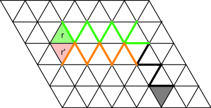
Figure 3: (Color online) Strings of electric field operators (thick lines), $S_{\mathbf{r}}$ and $S_{\mathbf{r^{\prime}}}$ that create or remove ${\mathchoice{\hbox{$\sf\textstyle Z\kern-3.99994ptZ$}}{\hbox{$\sf\textstyle Z\kern-3.99994ptZ$}}{\hbox{$\sf\scriptstyle Z\kern-2.10002ptZ$}}{\hbox{$\sf\scriptscriptstyle Z\kern-0.99998ptZ$}}}_{2}$ fluxes in the plaquettes indicated by the shaded triangles. For two arbitrary fluxes the corresponding strings have a common part (full lines) and individual parts (gray lines). Two individual parts form a contour that connects two fluxes. Each of these three substrings anticommutes with all others that results in the anticommutation of the flux creation operators (see text)

As for the square lattice, it is fruitful to introduce string-like operators $S_{\mathbf{r}}$ which create or remove a ${\mathchoice{\hbox{$\sf\textstyle Z\kern-3.99994ptZ$}}{\hbox{$\sf\textstyle Z\kern-3.99994ptZ$}}{\hbox{$\sf\scriptstyle Z\kern-2.10002ptZ$}}{\hbox{$\sf\scriptscriptstyle Z\kern-0.99998ptZ$}}}_{2}$ flux on a plaquette labelled by a site $\mathbf{r}$ on the hexagonal dual lattice. This operator involves the product of $\mathcal{E}_{kl}$ on a contour that starts from a specific bond of the lattice, as shown on Fig. 3. For the gauge invariant states all such contours are equivalent, so this contour can be chosen arbitrarily. For instance, one can choose the contours that first go up and then left toward the plaquette $r$. Using the fact that electric operators on nearby links anti-commute, we have:

$$S_{\mathbf{r}}^{2}=(-1)^{l(\mathbf{r})-1}$$ (12)

where $l(\mathbf{r})$ is the length of the contour $\mathbf{r}$, namely it is the total number of electric operators involved in the construction of $S_{\mathbf{r}}$. Because a gauge transformation changes the length of the contour by an even number, the right-hand side of Eq. (12) depends only on the parity, $[\mathbf{r}]\equiv(l(r)-1)\operatorname{mod}2$, of the plaquette $\mathbf{r}$ and not on the contour leading to it. Note that $S_{\mathbf{r}}$ is not always a hermitian operator, since

$$S_{\mathbf{r}}^{\dagger}=(-1)^{[\mathbf{r}]}S_{\mathbf{r}}$$ (13)

The commutation rules obeyed by these string operators are the following:

$$\{S_{\mathbf{r}},S_{\mathbf{r^{\prime}}}\}=2\delta(\mathbf{r},\mathbf{r^{\prime}})(-1)^{[\mathbf{r}]}$$ (14)

This crucial property which exhibits a clear fermionic behavior can be proved in two ways. First, one can deform the contours so that they overlap between point $0$ and $\mathbf{r}$. Then $S_{\mathbf{r^{\prime}}}=S_{\mathbf{r^{\prime},r}}S_{\mathbf{r}}$ where $S_{\mathbf{r^{\prime},r}}$ is the contour beginning at $\mathbf{r}$ and ending at $\mathbf{r}^{\prime}\mathrm{.}$ This contour $S_{\mathbf{r^{\prime},r}}$ contains exactly one electric field operator namely its first one, which anticommutes with the last electric field operator entering in $S_{\mathbf{r}}$, so operators $S_{\mathbf{r^{\prime},r}}$ and $S_{\mathbf{r}}$ anticommute which proves (14). Alternatively, one can write the original $S$ operators as products $S_{\mathbf{r}}=\widetilde{S}_{\mathbf{r}}S_{0}$ and $S_{\mathbf{r}^{\prime}}=\widetilde{S}_{\mathbf{r}^{\prime}}S_{0}$  where $S_{0}$ is the product of electric field operators on the common part of the contour leading to plaquettes $\mathbf{r}$ and $\mathbf{r}^{\prime}$, see Fig. 3. The operators $\widetilde{S}_{\mathbf{r}}$ and $S_{0}$ have exactly one pair of nearest neighboring electric fields, so they anticommute: $\{\widetilde{S}_{\mathbf{r}^{\prime}},S_{0}\}=\{\widetilde{S}_{\mathbf{r}},S_{0}\}=0$. Thus, $S_{\mathbf{r}}S_{\mathbf{r^{\prime}}}=-S_{0}^{2}\widetilde{S}_{\mathbf{r}}\widetilde{S}_{\mathbf{r}^{\prime}}$ and $S_{\mathbf{r}^{\prime}}S_{\mathbf{r}}=-S_{0}^{2}\widetilde{S}_{\mathbf{r}^{\prime}}\widetilde{S}_{\mathbf{r}}$, further, noticing that the operators $\widetilde{S}_{\mathbf{r}}\widetilde{S}_{\mathbf{r}^{\prime}}$ contain exactly one pair of anticommuting electric fields, we get (14).

A very important property of this model restricted to its physical subspace defined above is that local electric operators on link $(kl)$ are simply related to bilinear expressions of the form $S_{\mathbf{r}}S_{\mathbf{r^{\prime}}}$ where the plaquettes $\mathbf{r}$ and $\mathbf{r^{\prime}}$ are located on both sides of the link $(kl)$. If $\mathbf{r}$ and $\mathbf{r^{\prime}}$ are nearest neighbor plaquettes, we have:

$$S_{\mathbf{r}}=\mathcal{E}_{kl}S_{\mathbf{r^{\prime}}}$$ (15)

which is a direct consequence of the definition of string operators. Thus,

$$\mathcal{E}_{kl}=(-1)^{[\mathbf{r}^{\prime}]}S_{\mathbf{r}}S_{\mathbf{r^{\prime}}}$$ (16)

The last stage is to introduce Majorana fermions $\chi_{\mathbf{r}}$ related to string operators by:

$$S_{\mathbf{r}}=i^{[\mathbf{r}]}\chi_{\mathbf{r}}$$ (17)

With this definition, it is easy to check that:

$$\chi_{\mathbf{r}}^{\dagger} =\chi_{\mathbf{r}}$$ (18)

$$\{\chi_{\mathbf{r}},\chi_{\mathbf{r^{\prime}}}\} =2\delta_{\mathbf{r},\mathbf{r^{\prime}}}$$ (19)

Eq. (16) becomes:

$$\mathcal{E}_{kl}=i\chi_{\mathbf{r}}\chi_{\mathbf{r^{\prime}}}$$ (20)

if site $\mathbf{r}^{\prime}$ is even ($[\mathbf{r}^{\prime}]=0$) and site $\mathbf{r}$ is therefore odd.

The electrical part of the Hamiltonian thus maps into the hopping of Majorana fermions. The full Hamiltonian includes also the magnetic field part. In case of ${\mathchoice{\hbox{$\sf\textstyle Z\kern-3.99994ptZ$}}{\hbox{$\sf\textstyle Z\kern-3.99994ptZ$}}{\hbox{$\sf\scriptstyle Z\kern-2.10002ptZ$}}{\hbox{$\sf\scriptscriptstyle Z\kern-0.99998ptZ$}}}_{2}$ model it is given by the operator that takes two values depending on the flux in a given plaquette, so a general function $f(\Phi)$ from (9) is reduced to a linear function $f(\Phi)=\mu\Phi$. Writing the Majorana fermion as a sum of two usual fermion operators $\chi=c+c^{\dagger}$, we see that the total fermion number $c^{\dagger}c$ changes by $\pm 1$ by the flux creation operator, so in the fermion language the full Hamiltonian becomes:

$$H=-i\sum_{(\mathbf{r},\mathbf{s})}(c_{\mathbf{r}}+c_{\mathbf{r}}^{\dagger})(c_{\mathbf{s}}+c_{\mathbf{s}}^{\dagger})+\mu\sum_{\mathbf{r}}c_{\mathbf{r}}^{\dagger}c_{\mathbf{r}}$$

where the indices $\mathbf{r},\mathbf{s}$ run over the sites of the dual (hexagon) lattice and the first sum goes over all nearest neighbours on this lattice. The spectrum of the excitations

$$E(k)=\sqrt{\mu^{2}+|t(k)|^{2}}\pm|t(k)|$$ (21)

where $t(k)$ is spectrum of fermions on the honeycomb lattice with a purely nearest neighbour hopping Hamiltonian $H_{t}=\sum_{(\mathbf{r},\mathbf{s})}c_{\mathbf{r}}^{\dagger}c_{\mathbf{s}}$. To compute $t(k)$ we choose elementary cell consisting of two sites, for instance the ones that belong to the same vertical bond. In momentum space the Hamiltonian becomes a matrix $H=c_{a,k}^{\dagger}K_{ab}c_{b,k}$ with

$$K=\left(\begin{array}[c]{cc}0&1+e^{i\mathbf{k\xi}}+e^{i\mathbf{k\eta}}\\ 1+e^{-i\mathbf{k\xi}}+e^{-i\mathbf{k\eta}}&0\end{array}\right)$$

where $\mathbf{\xi=(}\frac{\sqrt{3}}{2},\frac{3}{2})$, $\mathbf{\eta=(-}\frac{\sqrt{3}}{2},\frac{3}{2})$ are unit vectors of the lattice of vertical bonds. We get

$$t(k)=\sqrt{1+4\cos\left(\frac{\sqrt{3}}{2}k_{x}\right)\cos\left(\frac{3}{2}k_{y}\right)+4\cos^{2}\left(\frac{\sqrt{3}}{2}k_{x}\right)}$$

In the absence of magnetic term the spectrum has dispersionless mode and a dispersive one which has zero only at the isolated Fermi points $(\pm 4\pi/(3\sqrt{3}),0)$, $(\pm 2\pi/(3\sqrt{3}),2\pi/3)$. Near the Fermi point the spectrum is linear $E(k)=3|k|$. In the presence of magnetic term two things happen: the dispersive mode acquires a gap $2\mu$, near the Fermi point the spectrum becomes massive $E(k)=\sqrt{(3/2)^{2}|k|^{2}+\mu}+(3/2)|k|$ and the dispersionless mode acquires $k$-dependence with the gap $\sqrt{\mu^{2}+9}-3.$

The presence of a dispersionless band for $\mu=0$ is directly connected to the presence of a set of local symmetries in the model. Indeed, if we introduce the Majorana operators $\widetilde{\chi}=i(c-c^{\dagger})$, they satisfy:

$$\widetilde{\chi}_{\mathbf{r}}^{\dagger} =\widetilde{\chi}_{\mathbf{r}}$$ (22)

$$\{\widetilde{\chi}_{\mathbf{r}},\widetilde{\chi}_{\mathbf{r^{\prime}}}\} =2\delta_{\mathbf{r},\mathbf{r^{\prime}}}$$ (23)

$$\{\chi_{\mathbf{r}},\widetilde{\chi}_{\mathbf{r}}\} =0$$ (24)

As a result, $\widetilde{\chi}_{\mathbf{r}}$ commutes with $H$ for any $\mathbf{r}$, therefore providing a set of non-commuting local symmetries which are destroyed by the presence of a magnetic term $\mu$.

IV Edge States

An interesting feature of the present model is that it exhibits edge states localized around boundaries. This is known to be a general property of Chern-Simons theories Witten89 , but an advantage of a lattice gauge theory with a discrete gauge group over a model defined on continuous space is to yield a finite dimensional Hilbert space. Therefore, we do not require any sophisticated analysis to specify boundary conditions. In the presence of a boundary, the definition of basic operators $\mathcal{E}_{kl}^{\pm}$ and $\mathcal{T}_{kl}^{\pm}$ for a link $kl$ along the boundary is the same as before, with the exception that the associated phase-factor only involves a smaller set of vector potentials $A_{mn}$ attached to the neighboring links lying inside the system. It is then easy to check that this does not modify the basic commutation relations between these operators. In particular, we shall still concentrate here on the $n=2$ case where nearby local field translation operators anticommute. The gauge generators $U_{k}$ located at site $k$ is still the product of all $\mathcal{T}_{kl}^{\pm}$ operators such that $kl$ lies inside the system. As illustrated on Fig. 4 this implies that $U_{k}$ and $U_{l}$ still commute when at least site $k$ or $l$ is not on the boundary, but they now anticommute if $k$ and $l$ are nearest neighbor sites both located on the boundary. This holds for most possible shapes of the boundary, with few exceptions which are depicted on Fig. 4. The striking consequence of this is that it is no longer possible to diagonalize simultanenously all local gauge generators $U_{k}$ belonging to the same boundary. In particular, gauge singlets no longer exist since they are replaced by degenerate multiplets corresponding to projective representations of the gauge group associated to boundary sites.

Figure 4: (Color online) Commutation relations between gauge generators attached to boundary sites in the ${\mathchoice{\hbox{$\sf\textstyle Z\kern-3.99994ptZ$}}{\hbox{$\sf\textstyle Z\kern-3.99994ptZ$}}{\hbox{$\sf\scriptstyle Z\kern-2.10002ptZ$}}{\hbox{$\sf\scriptscriptstyle Z\kern-0.99998ptZ$}}}_{2}$ Chern-Simons model. We show various possible edge shapes and indicate the corresponding opening angle expressed in degrees. For each situation, we display the gauge generators for a pair of nearest-neighbor sites. These generators involve the electric operators originating from a given site, and are depicted either as full (red) thick lines or dashed (blue) thick lines. For all situations appearing on the outer boundary of the lattice, these gauge generators are found to anticommute, which induces degenerate multiplets for the gauge symmetry. An exception to this rule is the $-60$ cusp shown on an inner hole for which the two nearby generators commute.

Let us now describe these multiplets in some detail. For this, we consider a finite triangular lattice with an outer boundary, and possibly with some inner holes, each of them bringing its own boundary. We assume that these holes are not too close from each other, so that local gauge generators associated to sites belonging to two different boundaries always commute. This assumption allows us to treat each boundary separately from the others. To simplify the discussion, we shall consider first the edge without $-60$ degrees turns that contains an even number $L$ of sites, which will be labelled by indices $n$ running from 1 to $L$. We suppose that fluxes in each plaquette and through each inner hole have been fixed, thereby concentrating on the degrees of freedom attached to gauge transformations. We may then associate to our boundary a Hilbert space containing $2^{L}$ independent states. In order to construct irreducible representations of the boundary gauge-group, we have to find a maximal subset of mutually commuting generators, which are then diagonalized simultaneously. Such set may be chosen as follows: take first generators $U_{2n}$ on even sites, and add then a global gauge generator $\prod_{n=1}^{L}U_{n}$ for the boundary. This yields $2^{1+L/2}$ possible sets of quantum numbers corresponding to:

$$U_{2n}|\Psi\rangle =\tau_{2n}|\Psi\rangle$$ (25)

$$\prod_{n=1}^{L}U_{n}|\Psi\rangle =\tau|\Psi\rangle$$ (26)

where eigenvalues $\tau_{2n}$ and $\tau$ can be $\pm 1$. We may still interpret $\tau$ as the total ${\mathchoice{\hbox{$\sf\textstyle Z\kern-3.99994ptZ$}}{\hbox{$\sf\textstyle Z\kern-3.99994ptZ$}}{\hbox{$\sf\scriptstyle Z\kern-2.10002ptZ$}}{\hbox{$\sf\scriptscriptstyle Z\kern-0.99998ptZ$}}}_{2}$ charge of matter induced on the boundary by the Chern-Simons term. Starting from a common eigenstate $|\Psi\rangle$ as above, applying $U_{2n+1}$ produces a new eigenstate in which $\tau_{2n}$ and $\tau_{2n+2}$ have changed sign simultaneously. Note that we have:

$$\prod_{n=1}^{\frac{L}{2}}U_{2n-1}|\Psi\rangle=\tau\prod_{n=1}^{\frac{L}{2}}\tau_{2n}|\Psi\rangle$$ (27)

so only $(L/2)-1$ generators located on odd sites act independently. We therefore generate a $2^{(L/2)-1}$ dimensional irreducible multiplet, so the Hilbert space attached to the boundary splits into $2^{(L/2)+1}$ such degenerate subspaces.

The above construction provides a basis in each multiplet for which $U_{2n}$ is represented by a diagonal matrix, whereas $U_{2n+1}$’s play the role of raising or lowering operators. A convenient way to visualize these multiplets is to describe them in terms of an effective spin 1/2 model, attached to even boundary sites. This correspondence is given by:

$$U_{2n} =\tau_{2n}^{z},\;\;\;(1\leq n\leq\frac{L}{2})$$ (28)

$$U_{1} =\tau_{L}^{x}\tau_{2}^{x}$$ (29)

$$U_{2n-1} =\tau_{2n-2}^{x}\tau_{2n}^{x},\;\;\;(2\leq n\leq\frac{L}{2}-1)$$ (30)

$$U_{L-1} =\tau\left(\prod_{n=1}^{\frac{L}{2}}\tau_{2n}^{z}\right)\tau_{L-2}^{x}\tau_{L}^{x}$$ (31)

A given multiplet corresponds to a fixed eigenvalue for $\prod_{n=1}^{\frac{L}{2}}\tau_{2n}^{z}$, so that the number of independent Ising spins is only $(L/2)-1$ as discussed above. Note that these conclusions apply to sufficiently large holes in the lattice. For very small holes consisting of two triangles glued together to form a rhombus (and of course for a single triangle itself) all boundary operators commute. The first pair of anticommuting operators appears in a trapezoidal hole shown in Fig. 4. This hole carries an effective spin $1/2$ degree of freedom because it is possible to diagonalize all gauge generators except one. Note that in this special case the product $\prod_{n=1}^{5}U_{n}$ anticommutes with the two local generators on upper sites, so the corresponding charge is no longer a conserved quantum number. In larger holes, such as hexagon, all nearest neighbor gauge generators anticommute. For instance, the boundary matter of elementary hexagon can be described as an effective system composed of two spins 1/2.

What is the interaction between these new matter-like degrees of freedom and the fluxons described in the previous section? Suppose first that these fluxons are not allowed to jump accross boundaries. This corresponds to a Hamiltonian where the electrical operators attached to boundary links are removed. The only interaction between the two sets of degrees of freedom occurs via the usual Aharonov-Casher phase-factor for fluxons going around inner holes. Each hole generates an effective ${\mathchoice{\hbox{$\sf\textstyle Z\kern-3.99994ptZ$}}{\hbox{$\sf\textstyle Z\kern-3.99994ptZ$}}{\hbox{$\sf\scriptstyle Z\kern-2.10002ptZ$}}{\hbox{$\sf\scriptscriptstyle Z\kern-0.99998ptZ$}}}_{2}$ orbital magnetic field which produces an adiabatic phase $\phi$ related to the ${\mathchoice{\hbox{$\sf\textstyle Z\kern-3.99994ptZ$}}{\hbox{$\sf\textstyle Z\kern-3.99994ptZ$}}{\hbox{$\sf\scriptstyle Z\kern-2.10002ptZ$}}{\hbox{$\sf\scriptscriptstyle Z\kern-0.99998ptZ$}}}_{2}$ charge by $e^{i\phi}=\tau$. This effect does not disturb the internal states of the boundaries which remain constants of motion. A stronger interaction occurs when fluxons are allowed to cross boundaries (that is to disappear from a boundary placquette). A simple description of this interaction is possible if a fluxon moves around a closed loop which crosses twice a given boundary. In this process, the final internal state of the boundary is connected to the initial one by applying the product of all local boundary gauge generators which are also enclosed in the closed loop. In the example of a hole with the shape of an elementary hexagon, these scattering processes can be simply expressed as products of operators taken in the set $\tau^{z}_{2},\tau^{x}_{2},\tau^{z}_{4},\tau^{x}_{4}$. In connection with the idea of topological quantum computation, we may wonder if these well defined operations can be used as a physical basis for qubits. The problem with this idea is that local gauge symmetry operators induce transitions between the various states of this effective spin system attached to the boundary. Since in any real implementation, noise acts through basically any local operator, such states cannot be protected from environment-induced decoherence. If we now consider the effect of either a large boundary, or many small inner holes, on the fluxon dynamics, we see that these processes tend to entangle fluxon states with an effective environment associated to boundary matter, resulting in the absence of long-ranged phase coherence for the Majorana fermions describing the fluxons. It is also very unlikely that the model preserves its integrabiblity, as soon as several fluxons and boundary matter are simultaneously present.

V Conclusions

In this paper, we have solved exactly a ${\mathchoice{\hbox{$\sf\textstyle Z\kern-3.99994ptZ$}}{\hbox{$\sf\textstyle Z\kern-3.99994ptZ$}}{\hbox{$\sf\scriptstyle Z\kern-2.10002ptZ$}}{\hbox{$\sf\scriptscriptstyle Z\kern-0.99998ptZ$}}}_{2}$ gauge theory with a Chern-Simons term on a triangular lattice by mapping the gauge-invariant subspace into a free Majorana fermion system. These fermions keep track of the dynamics of local fluxes. In the absence of an energy cost to create a ${\mathchoice{\hbox{$\sf\textstyle Z\kern-3.99994ptZ$}}{\hbox{$\sf\textstyle Z\kern-3.99994ptZ$}}{\hbox{$\sf\scriptstyle Z\kern-2.10002ptZ$}}{\hbox{$\sf\scriptscriptstyle Z\kern-0.99998ptZ$}}}_{2}$ flux, the spectrum is very degenerate: it exhibits a flat band at zero energy and a dispersive one with a vanishing energy at isolated points on the Brillouin zone boundary. This picture is very similar to the solution found by Kitaev for a quantum spin 1/2 model on the hexagonal lattice Kitaev03 . In this model, he considered nearest-neighbor interactions of the form $(\mbox{\boldmath$\sigma$}_{i}.\mbox{\boldmath$n$}_{ij})(\mbox{\boldmath$\sigma$}_{j}.\mbox{\boldmath$n$}_{ij})$ where $\mathbf{n}_{ij}=\mathbf{e}_{x},\mathbf{e}_{y},\mathbf{e}_{z}$ depending on the unit vector joining sites $i$ and $j$. These operators have the same anticommutation properties as the local fluxon moving operators $\mathcal{E}_{kl}=i\chi_{\mathbf{r}}\chi_{\mathbf{r^{\prime}}}$ introduced in the Chern-Simons lattice gauge model. However, we have not found a way to establish a one to one mapping between these two models. We do not see any operator in Kitaev’s spin model which could be interpreted as a local fluxon number, since it would have to anticommute with the three components $\sigma^{x}$, $\sigma^{y}$, $\sigma^{z}$ of the local spin at any site. In our gauge theory, fluxons have to be created by non-local operators $S_{\mathbf{r}}$ associated to contours, so it does not seem easy to express them in terms of local spin operators.

The presence of a gapless spectrum in the absence of a magnetic energy term is reminiscent of the gapless phase found on a square lattice Doucot2005 ; Dorier2005 . On a square lattice, this ${\mathchoice{\hbox{$\sf\textstyle Z\kern-3.99994ptZ$}}{\hbox{$\sf\textstyle Z\kern-3.99994ptZ$}}{\hbox{$\sf\scriptstyle Z\kern-2.10002ptZ$}}{\hbox{$\sf\scriptscriptstyle Z\kern-0.99998ptZ$}}}_{2}$ Chern-Simons model can be mapped into a spin 1/2 model with anisotropic exchange interactions of the form $\sigma^{x}_{i}\sigma^{x}_{j}$ or $\sigma^{z}_{i}\sigma^{z}_{j}$ depending on the orientation of the link $ij$. Adding a magnetic term in the Chern-Simons theory is then equivalent to imposing a magnetic field along the $\mathbf{y}$ direction in the spin model. It would be interesting to check that it also induces a spectral gap. Unfortunately, such a magnetic field term does not commute with the non-local symmetry operators associated to rows and columns of the square lattice which were responsible for the two-fold degeneracy of all energy eigenstates.

Finally, we have shown explicitely that charged matter degrees of freedom are always induced along edges associated to the external boundary or to inner holes. These degrees of freedom appear naturally since the presence of an edge forces the representation of the local gauge symmetry to become projective, i.e. gauge generators attached to nearest neighbor sites both located along an edge do not commute. We have shown that these new degrees of freedom provide static Aharonov-Bohm fluxes for the orbital motion of fluxons, provided the latter are not allowed to cross edges. Transitions within these degenerate matter multiplets are induced by processes where a fluxon goes back and forth accross a boundary. Unfortunately, these multiplets are very sensitive to external noise acting through local operators, so it is unlikely they may serve the purpose of designing protected qubits.

It is an immediate extension of this work to add local static charges in the system and see how they interact with this fluid of Majorana fermions associated to fluxons. Very likely, the interaction will be of the Ahoronv-Casher type, which is too weak to induce a confining force for a pair of opposite charges. So again, we have a direct evidence that a Chern-Simons term distroys the confining regime expected in gauge theories with small magnetic energy in the absence of a Chern-Simons term Pisarski86 ; Affleck89 .

The most important question connected to protected quantum computation is the construction of similar models for a finite non-Abelian group Mochon2003 ; Mochon2004 . This is the subject of a forthcoming work.

Acknowledgments

We are thankful to M.V. Feigelman and A. Silva for the critical reading of the paper. LI is thankful to LPTHE, Jussieu for their hospitality while BD has enjoyed the hospitality of the Physics Department at Rutgers University. We thank A. Kitaev for kindly sending us his unpublished work on the honeycomb lattice which encouraged us to study the Chern-Simons theory on the triangular lattice. This work was made possible by support from NATO CLG grant 979979, NSF DMR 0210575.

References

- (1) E. Dennis, A. Kitaev, A. Landahl and J. Preskill, J of Math. Phys. 43, 4452 (2002).
- (2) A.M. Childs, E. Farhi and J. Preskill, Phys Rev. A 65, 012322 (2001).
- (3) J. Preskill, Proc. Roy. Soc. A 454, 385 (1998).
- (4) See, e.g. L.B. Ioffe, V.B. Geshkenbein, Ch. Helm and G. Blatter, Phys. Rev. Lett. 93, 057001 (2004) for the limits on Josephson junction qubit quality.
- (5) A.Yu. Kitaev, Ann. Phys. 303, 2 (2003).
- (6) C. Mochon, Phys. Rev. A 67, 022315 (2003).
- (7) C. Mochon, Phys. Rev. A 69, 032306 (2004).
- (8) B. I. Halperin, Phys. Rev. Lett. 52, 1583, (1984).
- (9) D. Arovas, J. R. Schrieffer, and F. Wilczek, Phys. Rev. Lett. 53, 722, (1984).
- (10) B. Doucot, M.V. Feigelman, L.B. Ioffe and A.S. Ioselevich, Phys. Rev. B 71, 024505 (2005).
- (11) J. Dorier, F. Becca and F. Mila, cond-mat/0501708 (2005).
- (12) E. Witten, Comm. Math. Phys. 121, 351, (1989)
- (13) A. Kitaev, Anyons in a spin model on the honeycomb lattice, cond-mat/0506438 (2005).
- (14) R. D. Pisarski, Phys. Rev. D34, 3851, (1986)
- (15) I. Affleck, J. Harvey, L. Palla, and G. Semenoff, Nucl. Phys. B328, 575, (1989)