Do Bose metals exist in Nature?

Abstract

We revisit the concept of superfluidity in bosonic lattice models in low dimensions. Then, by using numerical and analytical results obtained previously for equivalent spinless fermion models, we show that the gapless phase of 1D interacting bosons may be either superfluid or -remarkably- metallic and not superfluid. The latter phase -the Bose metal- should be, according to the mentioned results, a robust and stable phase in 1D. In higher dimensionalities we speculate on the possibility of a stable Bose metallic phase on the verge of a Mott transition.

1 Introduction

In the last decades there have been a lot of numerical and theoretical works on interacting Bose gas in lattice or continuous models.ceperley ; scalettar ; dmrgbose ; troyer ; sandvick ; fisher ; cazalilla The recent advance in the realization of optical lattices, where bosons are trapped on particular lattice sites and the interaction and the hopping parameters can be tuned continuously, has also opened a novel possibility to understand fundamental questions of many-body quantum mechanics, that can be experimentally checked with high degree of reliability and reproducibility. An important example is the realization of a Mott insulating state in a system with strong on site repulsion.greiner2d ; greiner3d

In this work we want to focus on an even more fundamental question, that is related to the concept of superfluidity. This concept deserves some discussion and generalization when considering a lattice model. The following discussion is not at all academic because, at present, lattice models can be realized with laser optical techniques, and the gedanken experiment we will discuss in the next section can be in principle realized experimentally.

2 The model on a ring

We consider a one dimensional Bose-Hubbard model in the ring shown in Fig.(1). The lattice ring is rotating with given angular velocity $\omega_{0}$ with respect to the environment $E$ which is considered here at rest for simplicity. Indeed in actual experiments the environment is usually rotating, but this does not change the forthcoming analysis, because our choice is just related to the reference frame.

The Hamiltonian can be generally written as:

$$H_{v}=\sum_{k}\epsilon_{k}a^{{\dagger}}_{k+v}a_{k+v}+\hat{V}$$ (1)

where $a^{{\dagger}}_{k+v}=\sum_{R}e^{-i(k+v)R}a^{{\dagger}}_{R}$ creates a boson in the ring with momentum ($\hbar=1$) $k+v$, $\epsilon_{k}$ is the dispersion of bosons in the lattice (e.g. $\epsilon_{k}=-2t\cos k$ for nearest neighbor hopping), periodic $\epsilon_{k+2\pi}=\epsilon_{k}$ and even $\epsilon_{k}=\epsilon_{-k}$, $\hat{V}$ any two-body interaction term depending only on the relative distance between bosons [e.g. $\hat{V}=U/2\sum_{R}n_{R}(n_{R}-1)$ for the Boson-Hubbard model, where $n_{R}=a^{{\dagger}}_{R}a_{R}$], thus is unaffected by the velocity $v=\omega_{0}L/\pi$ of the rotating frame. The total momentum in the reference system where the ring is at rest is given (modulo $2\pi$) by: $P=\sum_{k}ka^{{\dagger}}_{k+v}a_{k+v}$ and the momenta $k$ are obviously quantized according to the known relation $kL=2\pi n$. Strictly speaking in a lattice only the operator $e^{iP}$ is defined, but this does not change the forthcoming analysis. In the forthcoming sections $H_{0}$ will be indicated by $H$ for simplicity.

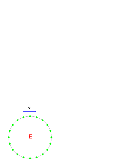
Figure 1: The model: the site positions are rotating with respect to the environment with given velocity $v$. The rotating sites are decoupled from the environment $E$, whereas the bosons can interact weakly with it, but are allowed to occupy only the site positions of the rotating ring.

The experimental issue to detect superfluidity is related to the following experiment. After an experimentally accessible time (the ring rotating and the environment at rest) will all the bosons be at rest relative to the environment (or equivalently will they move with an appropriate velocity with respect to the ring lattice positions)? If this is not the case we can speak about supefluidity, a fraction $\rho_{s}$ of all bosons decouple from the rest and remains uncoupled from the environment.

It is clear from the previous definition that superfluidity is related to the coupling to the environment (otherwise any finite momentum will be conserved for ever in the ring). Nevertheless it is possible to obtain a result that is independent of the interaction between the environment and the ring if the following three conditions are satisfied:

i) the thermodynamic limit $L\to\infty$ is considered,

ii) a finite temperature is given and the low temperature limit is considered after that the thermodynamic limit is employed,

iii) the model Hamiltonian provides a stable phase in the low energy spectrum, namely stable for small perturbation of the Hamiltonian itself.

The first two conditions are easily understood: only within the finite temperature canonical distribution $Z=Tre^{-\beta H}$ the momentum $e^{iP}$ can equilibrate even without considering the coupling with the environment, and the probability of each eigenstate of the isolated ring $H$ is given correctly by $e^{-\beta E_{i}}$, for a macroscopic system ($L\to\infty$), just when the coupling environment-ring is negligible with respect to the bulk $L$. The coupling environment-ring is used only to equilibrate the system and obtain a property-superfluidity- that characterizes the system itself and not its coupling with the environment (otherwise we could talk about ”superfluidity of capillary tubes” and not superfluidity of e.g. $He_{4}$). In order to achieve this consistent definition the Hamiltonian itself describing the system without environment has to define a stable phase of matter, namely a phase stable for small physical perturbations of the Hamiltonian, otherwise, clearly, the realization of a particular phase can obviously depend on the coupling environment-system.

In cold atoms experiments $L$, the number of sites, can be as large as $10^{5}$ and the thermodynamic limit at fixed temperature represents a realistic limit. It is important to emphasize that the physical zero temperature limit is highly non trivial in this respect. If we take first $\beta\to\infty$ and then $L\to\infty$ superfluidity cannot be tested because the lowest eigenstates of the Hamiltonian with non zero current have also a non trivial complex momentum $e^{iP}$ that is obviously conserved and no relaxation process can occur to the real ground state in a finite size system. If we explicitly consider a coupling system-environment as inlandau to induce current relaxation, it is clear that this process should be essentially equivalent to work in the thermodynamic limit with an arbitrary small temperature.

We conclude therefore that the correct limit for detecting zero temperature superfluidity is to take first $L\to\infty$ and then $\beta\to\infty$. This order of the limits leads indeed to the definition of superfluidity that is independent of the coupling system-environment, whenever this is possible, namely when (iii) is satisfied.

3 Free energy and thermodynamic equilibrium

In this section we revisit some basic notions in thermodynamics, by introducing the basic quantities that define the superfluid density. The following considerations are completely general and hold in any dimensionality D with minor changes, that we omit in the following.

In the thermodynamic equilibrium it is easy to show that the free energy:

$$F_{v}=-1/\beta\log(Tr~{}e^{-\beta H_{v}})$$ (2)

does not depend on $v$ for discrete values of $v=v_{n}=2\pi n_{L}/L$, with $n_{L}$ being an arbitrary integer. For large size $L$ this limitation is very weak because we can reach any finite velocity $v$ for $L\to\infty$ as , in this limit, the discrete velocity values merge in a continuum. Indeed for each $L$ a simple unitary transformation, commuting with the two-body interaction $\hat{V}$:

$$U=e^{-i\sum_{R}v_{n}R~{}n_{R}}$$ (3)

removes the velocity $v_{n}$ from $H$. This follows immediately after simple application of canonical commutation rules, implying that $\left[n_{R^{\prime}},a_{R}\right]=-\delta_{R,R^{\prime}}a_{R}$, so that $U^{{\dagger}}a_{k+v}U=a_{k}$, and finally $U^{{\dagger}}H_{v}U=H$ is easily obtained ($U^{{\dagger}}a^{{\dagger}}_{k+v}a_{k+v}U=(U^{{\dagger}}a^{{\dagger}}_{k+v}U)(U^{{\dagger}}a_{k+v}U)=a^{{\dagger}}_{k}a_{k}$ in the kinetic energy).

Using the above relation, it follows that the free energy:

$$F_{v}=-1/\beta\log(Tre^{-\beta H_{v}})=-1/\beta\log(TrU^{{\dagger}}e^{-\beta H_{v}}U)=-1/\beta\log(Tre^{-\beta U^{{\dagger}}H_{v}U})=F_{0}$$ (4)

does not depend on $v$ whenever $v=v_{n}$, namely when $U$ is defined. Notice that in the first step we have used the invariance of the trace under cyclic permutation.

From this relation we can expand the partition function in powers of $v$ because the mapping $k\to k+v_{n}$ is just a shift of the finite size momenta and the kinetic energy of $H_{v}$ can be recasted in the following form: $H=\sum_{k}\epsilon_{k-v_{n}}a^{{\dagger}}_{k}a_{k}$ We thus obtain upon performing simple differentiations:

$${dF\over dv} = -<J>_{v}+<K>v+O(v^{2})=0$$ (5)

$$J = \sum_{k}{de(k)\over dk}a^{{\dagger}}_{k}a_{k}$$ (6)

$$K = \sum_{k}{d^{2}e(k)\over dk^{2}}a^{{\dagger}}_{k}a_{k}$$ (7)

where the brackets $<O>_{v}$ ($<O>$) denote the finite temperature averages

$$<O>_{v}={TrOe^{-\beta H_{v}}\over Tre^{-\beta H_{v}}}$$

on the Hamiltonian of the rotating ring (non rotating ring, i.e. with $v=0$). Strictly speaking the previous differentiation in the free energy is not allowed because the possible velocities are quantized $v_{n}=2\pi n/L$ otherwise the unitary transformation $U$ is not properly defined. In a more rigorous way one can indeed consider that:

$$<J>_{v_{n}}=<U^{{\dagger}}JU>=<\sum_{k}{d\epsilon_{k}\over dk}|_{k+v_{n}}a^{{\dagger}}_{k}a_{k}>$$ (8)

In the latter equation we can expand ${d\epsilon_{k}\over dk}|_{k+v_{n}}={de(k)\over dk}+v_{n}{d^{2}e(k)\over dk^{2}}$ and use that $<J>=0$ in the canonical ensemble of the rotating ring because the current is odd under reflection and the Hamiltonian $H$ is even for $v=0$. This immediately implies the linear relation between the current flowing in the frame rotating with the ring and the corresponding velocity at thermal equilibrium:

$$<J>_{v_{n}}=<K>v_{n}+O(v_{n}^{2})$$ (9)

within ”weak” assumptions on the average boson occupation in momentum space $n_{k}=a^{{\dagger}}_{k}a_{k}$ (e.g. $1/L\sum_{k}{d^{3}e(k)\over dk^{3}}<n_{k}>$ is finite) that allows to neglect the $O(v_{n}^{2})$ term even for small but macroscopic velocities $v_{n}$. It has to be remarked here that the fundamental relation (9) is valid only at thermal equilibrium and this may be obtained only after an exceedingly large time. This is indeed the case when, for $L\to\infty$, superfluidity occurs. On the other hand whenever the relation (9) is fulfilled the current flowing in the ring is just representing the condition of thermal equilibrium: all the bosons by scattering with the environment eventually converge to an equilibrium state characterized by no charge flow in the environment frame.

We notice that a linear relation between the current and the velocity can be obtained within the linear response theory. The evaluation of $<J>_{v}$ for small $v$ is given by:

$$<J>_{v}=\left[\int\limits_{0}^{\beta}dt<J(t)J(0)>\right]v$$ (10)

where $J(t)=e^{tH}Je^{-tH}$. and can be obtained by simple expansion of the trace with simple and standard manipulations. Whenever the kernel $\alpha(0)$ relating the current response to an arbitrary small velocity is not equal to $<K>$ we will have a relation current velocity plotted in Fig(2). For any measurable finite velocity quantized as multiples of $2\pi/L$, there is no net current flow in the environment frame, implying that $<J>_{v}-<K>v=0(v^{2})$ at equilibrium, as expected. However for unphysically small values of the current the linear response may have a finite slope as shown in Fig.(2).

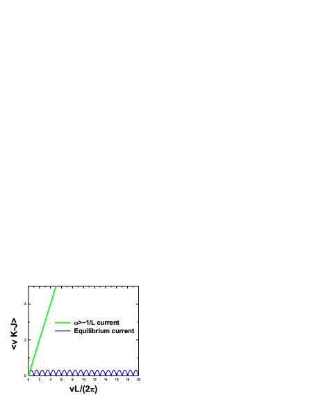
Figure 2: Equilibrium current in the environment frame as a function of the velocity $v$ of the rotating ring displayed in Fig.(1). The linear behavior occurs in an irrelevant region with exceedingly small velocity, certainly not measurable for large $L$, and in any case without any macroscopic current flowing in the environment frame.

3.1 Dynamical limit $\omega\to 0$

We are arguing in the following that the situation displayed in Fig.(2) is actually the common one for a superfluid ($L\to\infty$ finite temperature). The point is that in a superfluid, in order to obtain the equilibrium steady state solution where no net current is flowing in the environment frame, an exceedingly large time is necessary because an initial current can very slowly relax to the steady state. In order to understand this fact it is useful to remark that the experiments of superfluidity are usually done with time dependent velocity v (e.g. a torsional pendulumbishop ). If the frequency $\omega$ is much larger than the inverse relaxation time of the current we can safely assume that linear response theory can be applied and we should obtain in this case a perfectly linear relation between the frequency dependent current and the frequency dependent velocity:

$$J(\omega)=\alpha(\omega)v(\omega)$$ (11)

for either small or macroscopically measurable velocities as shown in the Fig.(2). The situation is in some sense similar to the evaluation of the conductivity of a metal. The expectation value of the current in presence of a static field $E$ leads always to zero conductivity because at thermal equilibrium no net current can flow. Indeed we have to take the appropriate limit, with a time dependent field and take $\omega\to 0$ after. This leads to the generally accepted Kubo formula for the conductivity.

In the superfluidity experiment, on the other hand, we have to consider the physical case when the relaxation time for the current becomes macroscopically large (infinite for infinite size) and the limit $\omega\to 0$ after the limit $L\to\infty$ at finite temperature $T$ leads to:

$$<J>_{v}=\left[\int\limits_{0}^{\beta}dt<J(t)J(0)>\right]v=(1-\rho_{s}/\rho)<K>v$$ (12)

where $\rho_{s}$ is the definition of superfluid density, being $\rho$ the total density of bosons. Indeed whenever $\rho_{s}>0$ only a fraction of the particles $1-\rho_{s}/\rho$ can be interpreted to have relaxed to the steady state in an experimentally accessible time. It is important to emphasize that this definition of superfluidity is experimentally testable but is not necessarily related to broken symmetry. Indeed in two dimensions, as well known, superfluidity can be detectedbishop and on the other hand there is no long range order at any finite temperature. Whenever there is long range order the situation is indeed more conventional because the superfluid density is directly related to the helicity modulus of the order parameterceperley .

4 Free bosons

In the free boson case, as shown in ceperley , it can be proved that $\rho_{s}$ coincides with the condensate fraction $\rho_{c}$ of particles that occupy the $k=0$ state with a macroscopic occupation. This calculation can be immediately generalized even for lattice models in any dimension $D$. Since the generalization is almost immediate we describe the basic steps in $D=1$ for convenience of notations and write down the explicit expression of $\rho_{s}$ as a function of $D$ only in the last equation.

For free bosons the current $J$ commute with the Hamiltonian and the linear response kernel $\alpha(0)$ is given by:

$$\alpha(0)=\beta<J^{2}>.$$ (13)

In fact the Hamiltonian, as well as $J$ (6), are diagonal in $k$ space $H=\sum_{k}\epsilon_{k}n_{k}$ $J=\sum_{k\neq 0}{d\epsilon_{k}\over dk}n_{k}$, where in the latter expression we have for convenience removed the $k=0$ vector in the summation because ${d\epsilon_{k}\over dk}=0$ for $k=0$ (the derivative of an even function is odd in $k$). Following Ref.ceperley , in order to evaluate Eq.(13) it is enough to compute the two body density matrix in momentum space:

$$<n_{k}n_{k^{\prime}}>=n^{B}_{k}n^{B}_{k^{\prime}}+\delta_{k,k^{\prime}}[(n^{B}_{k})^{2}+n_{k}^{B}]$$ (14)

where $n^{B}_{k}=1/[e^{(}\beta(\epsilon_{k}-\mu))-1]$ is the free boson occupation at finite temperature, and $\mu$ is the chemical potential used to require a given density $\rho$ of bosons $\rho={1\over L}\sum_{k}n^{B}_{k}=\rho_{c}+{1\over L}\sum_{k\neq 0}n^{B}_{k}$, where $\rho_{c}$ is just the condensate density. In this way the evaluation of $\alpha(0)$ can be readily performed and simplified, by using that i) $\sum_{k\neq 0}n^{B}_{k}{d\epsilon_{k}\over dk}=0$ again because of the reflection symmetry ii) as noted in Ref.ceperley $[(n^{B}_{k})^{2}+n_{k}^{B}]=-1/\beta{dn^{B}_{k}\over d\epsilon_{k}}$:

$$\alpha(0)=-\sum_{k\neq 0}\left({d\epsilon_{k}\over dk}\right)^{2}{dn^{B}_{k}\over d\epsilon_{k}}$$ (15)

We can now take the appropriate $L\to\infty$ limit to compute $\rho_{s}$ and $\rho$ by replacing the summation $1/L^{D}\sum_{k\neq 0}\to\int{dk^{D}\over(2\pi)^{D}}$ and obtain a closed form expression for $\rho_{s}$ (a simple integration by part is also left to the reader):

$$\rho_{s}/\rho={\rho_{c}\over\rho_{c}+{\int{dk^{D}\over(2\pi)^{D}}{d^{2}\epsilon_{k}\over dk_{x}^{2}}n^{B}_{k}\over{d^{2}\epsilon_{k}\over dk_{x}^{2}}|_{k_{x}=0}}}$$ (16)

It is interesting that $\rho_{s}\neq\rho_{c}$ in this case, but there is superfluid density only when there is a non zero condensate fraction and the other way around.

Thus $\rho_{s}=0$ for $\beta<\beta_{c}$ where $\beta_{c}$ is the inverse Bose-Einstein transition temperature that is finite in 3D but is infinite in 1D and 2D.

4.1 Zero temperature limit

In principle we can take first the limit $\beta\to\infty$ for the kernel $\alpha$ at any fixed size $L$. As we have emphasized before, this limit cannot test superfluidity and indeed is related to another physical quantity, the zero temperature Drude weight as established by Kohn long time agokohn :

$$D_{c}=\lim_{L\to\infty}{1\over L}\lim_{\beta\to\infty}(<K>-\alpha(0))$$ (17)

that distinguishes a metal from an insulator, but not a metal from a superfluid.

In the following the distinction between a Bose-metal from a Bose-superfluid is essentially analogous to the difference between a metal and a superconductor valid for electronic systemsscalapino : superconductors are obviously metal in the sense of infinite zero temperature conductivity but they also possess the non trivial property that the current can flow basically forever without dissipation at any finite temperature below $T_{c}$. Clearly, within this definition, if $T_{c}=0$, we can speak about a Bose-metal in the ground state because there is no measurable superfluid density for any $T>0$.

In order to show that the limit $\beta\to\infty$ before the thermodynamic limit is incorrect for the detection of superfluidity, it is enough to realize that, for free bosons, in the limit $\beta\to\infty$ at fixed $L$ the kernel $\alpha(0)\to 0$ because the current commute with the Hamiltonian and in the ground state $J=0$ so that $\alpha(0)=\beta<J^{2}>$ decays exponentially to zero for $\beta\to\infty$ due to the finite size gap $~{}1/L^{2}$ of the first excited state with non zero current. Thus we obtain that the Drude weight for free bosons is always finite and equal to $<K>$. Thus $D_{c}\neq 0$ in 1D and 2D even though at any finite temperature

$$<K>=\alpha(0)$$

for $L\to\infty$, implying $\rho_{s}=0$ for any $T>0$.

In our definition therefore, a free 1D or 2D Bose gas, is not a superfluid but a Bose metal. This Bose metal however is too much idealized to be considered realistic because interaction is always present and it is known that an arbitrary small interaction changes the spectrum of the excitations from quadratic to linear in momentum, and condition iii) for superfluidity is not satisfied. Thus the issue of the present paper on whether Bose metals can exist in a stable phase is not solved by the free boson example. Bose metals should exist in nature only if a small physical perturbation of the Hamiltonian does not change the qualitative features of the unperturbed phase.

Other definitions are known in the literature for a Bose-metaldoniach , but appear much more restrictive definitions than the present one.

5 Models with interaction in 1D

It is fortunate that the problem has been already studied in 1D and we can use convincing results obtained in other contextszotos ; andrei ; 1dbose . The calculation of $\rho_{s}$ was done with the correct order of limits in zotos . In this work the authors considered 1d-spinless fermions at half filling with nearest neighbor hopping, nearest $V$ and next-nearest neighbor $W$ repulsive interactions. This model, as well known, is equivalent to hard-core bosons with the same interaction coupling constants, because in 1D hard core bosons with nearest neighbor hopping are simply related to spinless fermion models with the same current-current response functions. The spinless fermion model, in the gapless phase, is relevant for our discussion and it was clearly found that indeed $\rho_{s}>0$ for $T>0$ as long as $W=0$ and $V>0$. However the authors claim that, an infinitesimal small coupling $W$ provides a vanishing $\rho_{s}$ at any finite temperature because-they argue- the model is no longer integrable by Bethe ansatz. In this case the zero temperature limit of $\rho_{s}$ does not coincide with the zero temperature Drude weight, that is generally finite in any gapless 1D spinless fermion phase, because it is related to the low-energy zero-temperature properties of the model.

If we agree with the conclusions of Ref.zotos , that are based on calculations on periodic rings with $\simeq 20$ sites, the model containing nearest and next-nearest neighbor repulsion is a Bose metal for any non zero $V,W>0$.

Indeed the conclusion of the workzotos is more general and , translated in the boson language, implies quite generally that 1D Bose metals do exist in the gapless phase. According to the authors conjecture, that is still under debate, $\rho_{s}=0$ for $T>0$ in all models that are non integrable with Bethe ansatz (e.g. also the celebrated Bose-Hubbard model falls in this class if we extend this conjecture also to bosonic models). A more clear argument was given in Ref.andrei , where the absence of a finite Drude weight ($\rho_{s}$) at finite temperature was predicted in all 1D models that do not have some conserved current. Essentially, in lattice models, the current can decay due to Umklapp-processes and a finite conductivity is expected at finite temperature, a condition that is incompatible with a finite $\rho_{s}$ (which implies a $\delta-$ function $\omega=0$ response and therefore an infinite finite temperature conductivity). The condition of integrability may instead allow for some conserved current, but it is also possible in principle that some conserved current can be realized even in non-integrable models.kawakami Recently a more clear numerical evidence was also given that in a generic 1D model with frustration $\rho_{s}$ is zero at finite temperature even in the gapless phase.1dbose

We do not want to enter in this subtle discussion on what is the right criterion that allows a finite $\rho_{s}$ at finite temperature, but from what is known so far, it appears that only very particular lattice models obtained with fine tuning of coupling constants can represent 1D Bose superfluid and that the generic gapless phase is instead a Bose metal, at least for hard core boson models. Moreover, in this case, the superfluid phase obtained at particular coupling strengths do not certainly satisfy property (iii) and superfluidity may be detected only for suitable and very particular environment-system coupling.

6 Conclusion

We have formulated a consistent definition of superfluidity valid for lattice and continuous models in any dimensionality that relates $\rho_{s}$-the superfluid density-to the linear response current-current correlation calculated at finite temperature. This formulation agrees with the Pollock-Ceperleyceperley one based on the winding number, provided the correct order of limit is taken: first the thermodynamic limit and then the zero temperature limit, relevant for ground state properties. In the opposite order of limits we have shown that the so called zero temperature Drude weight is obtained, but this can be finite both for a Bose-metal and for a Bose-superfluid. The discrimination between the two can be obtained at finite temperature within the present formulation or by using the Scalapino-criterion that can be worked out directly at $T=0$scalapino . Both criteria coincide in the $T\to 0$ limit for model systems where the solution is known, but the latter one cannot be applied in 1D because it is not possible to define a transverse field in this case.

The main conclusion of our approach is that in 1D a generic gapless phase may be metallic and not superfluid, namely a very peculiar and interesting interacting phase - the Bose metal- with finite zero temperature Drude weightsemimetal but no superfluid density.

In many recent papers the possibility to have this type of Bose metal has not been considered yet, especially in 1Dfisher ; scalettar ; cazalilla ; dmrgbose , where it has been usually assumed that the gapless phase is superfluid. This attribute was originally used to characterize the classical 2D phase corresponding to the 1D zero temperature quantum model. This was certainly correct but may be clearly misleading, because the superfluidity of the 2D classical model may be not related to the superfluidity of the corresponding quantum model at low temperature.

In this work we have shown that 1D hard-core boson interacting-systems should be Bose metals in the generic gapless phase, simply because for these models superfluidity cannot be detected at any $T>0$ (apart for the mentioned exceptions), even when the Drude weight is non zero in the ground state.

Based on the above results, it appears possible that this Bose metal phase can be extended also to some model without the hard core constraint, because this constraint should not play an important role at low energycazalilla . The seminal work by Fisher and coworkers on the mapping of the 1D zero temperature Bose-Hubbard model to a classical 2D model at finite temperature is perfectly valid as far as the critical behavior at the transition is concerned. However, in this mapping, the superfluid density of the classical model (that can be finite below the Kosterlitz-Thouless transition temperature) is related to the Drude-weight of the quantum zero temperature model and not-obviously- to its finite temperature superfluid density. This quantity can be in principle different from the Drude weight, even at arbitrary small temperature, whenever the system is indeed metallic and not superfluid. It is also clear that the analytical calculation of the ”superfluid density” reported in Ref.(cazalilla ) for Luttinger liquids refers instead to the zero temperature Drude weight which is obviously finite, but does not necessarily imply superfluidity. On the other hand in the numerical calculation reported in Ref.scalettar , no finite size scaling is attempted at fixed temperature. Based on these considerations it appears important to improve further the numerical results of the 1D bosonic models with soft or hard core constraint by using recent more accurate and powerful techniquessandvick , that can be extended to much larger system sizes. This may allow to establish more accurately the nature of the gapless phases of 1D Bose models.

In 2D close to a metal-insulator transition we have recently speculatedcapello on the possibility to have a non Fermi liquid phase before the Mott-insulating phase. In the boson language this possibility can be realized whenever the phonon velocity $c$ in the superfluid phase goes to zero before the Mott transition. In such a case an anomalous phase with finite zero temperature Drude weight but no superfluid density should appear between the Mott insulator and the superfluid. In this phase it can be also shown that there is no condensate, using a known relation based on the generalized indetermination principle.stringari In the language of spin liquids the Bose-metal is just a gapless spin-liquid of the type stabilized in the frustrated $J_{1}-J_{2}$ modelrainbow . Although in dimension higher than one all these examples are clearly not well established because they are based on the variational approximation, we believe that, since in 1D the Bose (spin) liquid is stable at least in hard-core boson models, it is worth to consider this phase as a possible phase of matter even in higher dimensionality and especially in 2D.

References

- (1) E. L. Pollock and D. M. Ceperley Phys. Rev. B 36, 8343 (1987).
- (2) G. G. Batrouni, R. T. Scalettar and G. T. Zimanyi Phys. Rev. Lett. 65, 1765 (1990), ibidem Phys. Rev. B 46, 9051 (1992).
- (3) L. I. Plinak, M. K. Olsen, and M. Fleishlauer Phys. Rev. A 70, 013611 (2004).
- (4) S. Wessel et al. Phys. Rev. A 70, 053615 (2004).
- (5) A. Sandvik, Phys. Rev. B 56, 11678 (1997).
- (6) M. P. A. Fisher et al Phys. Rev. B 40, 546 (1989).
- (7) M. A. Cazalilla J. Phys. B 37, S1 (2004).
- (8) M. Greiner et al. Nature (London) 415, 39 (2002).
- (9) M. Greiner et al. Nature (London) 426, 537 (2003).
- (10) Landau long time ago, have defined a criterion of superfluidity that is valid in the ground state and is based on the coupling environment at rest- and system at finite velocity . See e.g. E. M. Lifs̈its and L. P. Pitaeskiï ”Statistical Physics: Theory of the condensed state” Pergamon Press Oxford (1980). Unfortunately this criterion cannot be applied to lattice models, because there is no Galilean invariance.
- (11) J. E. Berthold, D. J. Bishop and J. D. Reppy Phys. Rev. Lett. 39, 348 (1977).
- (12) W. Kohn, Phys. Rev. 133, A171 (1964).
- (13) D. J. Scalapino, S. R. White and S. Zhang Phys. Rev. B 47, 7995 (1993).
- (14) D. Das and S. Doniach Phys. Rev. B 60, 1261 (1999), ibidem 64, 134511 (2001).
- (15) X. Zotos and P. Prelovs̈ek Phys. Rev. B 53, 983 (1996).
- (16) A. Rosch and N. Andrei, Phys. Rev. Lett. 85, 1092 (2000).
- (17) F. H. Meisner et al. Phys. Rev B 68, 134436 (2003).
- (18) S. Fujimoto and N. Kawakami, Phys. Rev. Lett. 90, 197202 (2003).
- (19) Indeed the Drude weight can be also zero , though with no resistivity at zero temperature as in semimetals. In this case it is more appropriate to name this phase ”Bose semimetallic phase”.
- (20) M. Capello et al. cond-mat/0509062.
- (21) L. Pitaevskii and S. Stringari, Phys. Rev. B 47, 10915.
- (22) L. Capriotti et al. Phys. Rev. Lett. 87, 097201 (2001).