Decoherence in weak localization II: Bethe-Salpeter calculation of Cooperon

Abstract

This is the second in a series of two papers (I and II) on the problem of decoherence in weak localization. In paper I, we discussed how the Pauli principle could be incorporated into an influence functional approach for calculating the Cooperon propagator and the magnetoconductivity. In the present paper II, we check and confirm the results so obtained by diagrammatically setting up a Bethe-Salpeter equation for the Cooperon, which includes self-energy and vertex terms on an equal footing and is free from both infrared and ultraviolet divergencies. We then approximately solve this Bethe-Salpeter equation by the Ansatz ${\tilde{C}}(t)={\tilde{C}}^{0}(t)e^{-F(t)}$, where the decay function $F(t)$ determines the decoherence rate. We show that in order to obtain a divergence-free expression for the decay function $F(t)$, it is sufficient to calculate $\tilde{C}^{1}(t)$, the Cooperon in the position-time representation to first order in the interaction. Paper II is independent of paper I and can be read without detailed knowledge of the latter.

I Introduction

This is the second in a series of two papers (I and II), in which we revisit the problem of decoherence in weak localization, using both an influence functional approach (paper I) and a Bethe-Salpeter equation for the Cooperon (paper II) to calculate the magnetoconductivity. The basic challenge is to calculate the interference between two time-reversed trajectories of an electron travelling diffusively in a Fermi sea and coupled to a noisy quantum environment, while taking proper account of the Pauli principle. In paper I paperI , we discussed how this could be done using an influence functional approach by dressing the spectrum of the noise field by “Pauli factors” [see Eq. (I.LABEL:subeq:theGreatReplacementa); throughout, “I” will indicate formulas from paper I]. Moreover, within the influence functional scheme we concluded that a divergence-free calculation of the decoherence rate can be obtained by expressing the Cooperon in the position-time representation as

$${\tilde{C}}(0,t)\simeq{\tilde{C}^{0}}(0,t)\,e^{-F(t)}\;,\quad F(t)=-\frac{{\tilde{C}}^{1}(0,t)}{{\tilde{C}^{0}}(0,t)}\;.$$ (1)

where $\tilde{C}^{1}(0,t)$ is the first-order term in an expansion of the full Cooperon ${\tilde{C}}(0,t)$ in powers of the interaction. [In the present paper, this statement will be made more precise: when reexponentiating, a part of $\tilde{C}^{1}(0,t)$ has to be omitted that can be determined, in a self-energy-only calculation, to contribute only to the prefactor of the Cooperon, see Sec. II.3.]

These conclusions of paper I rested entirely on the influence functional approach, and, in the discussion of the Pauli principle, relied on heuristic arguments. Though these are in accord with results derived elsewhereAAK ; AAG ; CS ; Abrahams ; vonDelft04 (as shown in Paper 1, Section LABEL:app:GZrelation), it is desirable to compare the approximations used and the results obtained so far against a treatment relying purely on diagrammatic perturbation theory, the framework within which most of our understanding of disordered metals to date has been obtained.

In the present paper II, we check and confirm the results mentioned above by diagrammatically setting up a Bethe-Salpeter equation for the Cooperon using standard Keldysh diagrammatic perturbation theory (using conventions summarized in vonDelft04 ), which includes self-energy and vertex terms on an equal footing and is free from both infrared and ultraviolet divergencies. We then show that this equation can be solved (approximately, but with exponential accuracy) with an Ansatz that is precisely of the form Eq. (1), and that the function $F(t)$ so obtained agrees with the form derived in paper I [Eq. (I.LABEL:exponentCLpaulimodified)].

The usual diagrammatic calculation of the Cooperon starts from a Dyson equation for a “self-energy-diagrams-only” version of the Cooperon,

$$\phantom{{\bm{q}}}{{\overline{\cal C}}{}}_{{\varepsilon},{\bm{q}}}^{\textrm{self}}(\omega)={\overline{\cal C}}{}^{0}_{\bm{q}}(\omega)\left[1+{\overline{\Sigma}}{}^{\textrm{self}}_{\varepsilon,{\bm{q}}}(\omega)\,{\overline{\cal C}}{}_{\varepsilon,{\bm{q}}}^{\textrm{self}}(\omega)\right]\;.$$ (2)

Here the Cooperon self-energy ${\overline{\Sigma}}{}^{\textrm{self}}_{\varepsilon,{\bm{q}}}$ includes only self-energy diagrams, in which interaction lines connect only forward to forward or backward to backward electron propagators; for these diagrams, the frequency labels along both the forward and the backward propagators are conserved separately, which is why the Dyson equation is a simple algebraic equation for ${\overline{\cal C}}{}_{\varepsilon,{\bm{q}}}^{\textrm{self}}(\omega)$. However, the Cooperon self-energy ${\overline{\Sigma}}{}^{\textrm{self}}_{\varepsilon,{\bm{q}}}(\omega)$ turns out to be infrared divergent in the quasi 2- and 1-dimensional cases. This problem is usually cured by inserting an infrared cutoff by hand (as reviewed in Section II.3 below). The results so obtained are qualitatively correct but, due to the ad hoc treatment of the cutoff, not very accurate quantitatively [e.g. in the first line of Eq. (21) for $\tilde{F}_{\varepsilon}^{\textrm{self}}(t)$ below the exponent is correct, but the prefactor is wrong by roughly a factor of 2 compared to Eq. (I.LABEL:eq:finalFrrw)].

Our goal in the present paper is to obtain, starting from a diagrammatic equation, results free from any cutoffs, infrared or ultraviolet, that have to be inserted by hand – the theory “should take care of its divergencies itself”. This can be achieved if the Cooperon self-energy is taken to include vertex diagrams, in which interaction lines connect forward and backward electron propagators. Since this brings about frequency transfers between the forward and the backward propagators, their frequency labels are no longer conserved separately. As a consequence, it becomes necessary to study a more complicated version of the Cooperon, ${\overline{\cal C}}{}^{\cal E}_{\bm{q}}(\Omega_{1},\Omega_{2})$, labeled by three frequencies, and governed not by a simple algebraic Dyson equation, but by a nonlinear integral equation, which we shall refer to as “Bethe-Salpeter equation”.

Finding an exact solution to the Bethe-Salpeter equation seems to be an intractable problem, which we shall not attempt to attack. Instead, we shall transcribe the Bethe-Salpeter equation from the momentum-frequency to the position-time domain, in which it is easier to make an informed guess for the expected behavior of the solution. Using the intuition developed in paper I within the influence-functional approach [summarized in Eq. (1) of the present paper], we shall make an exponential Ansatz for ${\tilde{C}}^{\varepsilon}(r_{12},t_{1},t_{2})$, the Cooperon in the position-time domain. We shall show that this Ansatz solves the Bethe-Salpeter equation with exponential accuracy, in the sense that improving the Ansatz would require terms to be added to the exponent that are parametrically smaller (in powers of $1/g$, $g$ being the dimensionless conductance) than the leading term in the exponent.

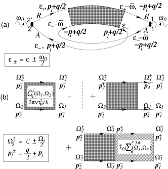
Figure 1: (a) Diagram for the weak localization correction to the AC conductivity, $\delta\sigma^{\textrm{WL}}(\omega_{0})$ [Eqs. (3)]. In contrast to the so-called “interaction corrections” to the conductivity, each current vertex is attached to both a retarded and advanced electron line. (b) Diagrammatic definition of full Cooperon $\bar{\cal C}_{\bm{q}}^{{\cal E}}(\Omega_{1},\Omega_{2})$, and schematic depiction of the Bethe-Salpeter equation (II.2) satisfied by it; ${\cal E}={\textstyle\frac{1}{2}}(\Omega_{j}^{+}+\Omega_{j}^{-})$ is the conserved average of the energies of the upper and lower lines, while $\Omega_{1}$ and $\Omega_{2}$ are the outgoing and incoming Cooperon frequencies (with $\Omega_{j}=\Omega_{j}^{+}-\Omega_{j}^{-}$). For the structure of the Cooperon self-energy ${\overline{\Sigma}}{}^{\textrm{full}}$ and details of our diagrammatic conventions, see Appendix A, Fig. 2.

II Setting up Bethe-Salpeter Equation for Cooperon

II.1 Various expressions for conductivity

The diagrammatic definition of the weak localization contribution to the AC conductivity of a quasi $d$-dimensional disordered conductor is given by Fig. 1(a), which corresponds to the following expression (cf. App. A of LABEL:AAK, or App. C of LABEL:vonDelft04):

$$\delta\sigma^{\textrm{WL}}_{d}(\omega_{0})=-{\sigma_{d}\over\pi\nu\hbar}\left\langle\tilde{\cal C}_{\textrm{cond}}^{\varepsilon,\omega_{0}}\right\rangle_{\varepsilon}\;,\qquad\phantom{.}$$ (3a)

$$\tilde{\cal C}_{\textrm{cond}}^{\varepsilon,\omega_{0}}=\!\!\int(d\,2{\widetilde{\omega}})\!\!\int(d{\bm{q}})\,\overline{\cal C}^{\varepsilon-{1\over 2}{\widetilde{\omega}}}_{\bm{q}}(\omega_{0}-{\widetilde{\omega}},\omega_{0}+{\widetilde{\omega}}),\qquad\phantom{.}$$ (3b)

where

$$\bigl{\langle}...\bigr{\rangle}_{\varepsilon}\equiv\int d\varepsilon\,{f({\varepsilon_{-}})-f({\varepsilon_{+}})\over\omega_{0}}\dots$$ (4)

denotes an average over $\varepsilon$, with $\varepsilon_{\pm}=\varepsilon\pm{\textstyle\frac{1}{2}}\omega_{0}$, and in the DC limit $\omega_{0}\to 0$ the weighting function reduces to $-f^{\prime}(\varepsilon)$, the derivative of the Fermi function $f(\varepsilon)=1/[e^{\varepsilon/T}+1]$. (In this paper, temperature is measured in units of frequency, i.e. $T$ stands for $k_{\rm B}T/\hbar$ throughout; likewise, although $\varepsilon$ will often be referred to as “excitation energy”, it stands for a frequency.)

The full Cooperon with general arguments, $\overline{\cal C}^{\cal E}_{\bm{q}}(\Omega_{1},\Omega_{2})$ is defined diagrammatically in Fig. 1(b): ${\cal E}$ is the average of the frequencies of the upper and lower electron lines, while $\Omega_{1}$ and $\Omega_{2}$ are the outgoing and incoming Cooperon frequencies, respectively. In the absence of external time-dependent fields, the average energy ${\cal E}$ is conserved between incoming and outgoing lines. The Cooperon needed for the AC conductivity in Fig. 1(a) has incoming upper and lower electron lines with energies ${\varepsilon_{+}}$ and ${\varepsilon_{-}}-{\widetilde{\omega}}$, and outgoing upper and lower electron lines with energies ${\varepsilon_{+}}-{\widetilde{\omega}}$ and ${\varepsilon_{-}}$, implying $\Omega_{1}=(\omega_{0}-{\widetilde{\omega}})$, $\Omega_{2}=(\omega_{0}+{\widetilde{\omega}})$ and ${\cal E}=\varepsilon-{\textstyle\frac{1}{2}}{\widetilde{\omega}}$, as used in Eq. (3b).

To make contact with the expression for the conductivity in the position-time representation used in paper I, we rewrite Eq. (3b) as

$$\tilde{\cal C}_{\textrm{cond}}^{\varepsilon,\omega_{0}} \equiv \int dt\,e^{i\omega_{0}t}\,\tilde{C}^{{\varepsilon_{+}}}(0,t)$$ (5a)

$$\tilde{C}^{\varepsilon_{+}}(0,t) \equiv \tilde{C}^{\varepsilon_{+}}(r_{12}=0;t_{1}={\textstyle\frac{1}{2}}t,t_{2}=-{\textstyle\frac{1}{2}}t)\;,\qquad\phantom{.}$$ (5b)

where $$\tilde{C}^{\varepsilon_{+}}({{\bm{r}}_{12}};t_{1},t_{2})$$ is a representation of the full Cooperon in an energy/position/two-time representation,

$$\tilde{C}^{\varepsilon_{+}}({{\bm{r}}_{12}};t_{1},t_{2}) = \int(d{\bm{q}})(d\Omega_{1})(d\Omega_{2})\,e^{i[{\bm{q}}{\bm{r}}_{12}-\Omega_{1}t_{1}+\Omega_{2}t_{2}]}\,$$ (5d)

$$\times\;{\overline{\cal C}}{}_{\bm{q}}^{{\varepsilon_{+}}-{1\over 2}\Omega_{2}}(\Omega_{1},\Omega_{2})\;,$$

$$= \int(d{\bm{q}})(d\,2{\widetilde{\omega}})(d\omega)\,e^{i[{\bm{q}}{\bm{r}}_{12}-\omega t_{12}+{\widetilde{\omega}}\tilde{t}_{12}]}\,$$

$$\times\;{\overline{\cal C}}{}_{\bm{q}}^{{\varepsilon_{+}}-{1\over 2}({\widetilde{\omega}}+\omega)}(\omega-{\widetilde{\omega}},\omega+{\widetilde{\omega}})\;,$$

where $r_{12}=r_{1}-r_{2}$, $t_{12}=t_{1}-t_{2}$, $\tilde{t}_{12}=t_{1}+t_{2}$, $\omega={\textstyle\frac{1}{2}}(\Omega_{2}+\Omega_{1})$ and ${\widetilde{\omega}}={\textstyle\frac{1}{2}}(\Omega_{2}-\Omega_{1})$. The $\int dt$ time integral in Eq. (5a) sets $\omega=\omega_{0}$ and hence ${\varepsilon_{+}}-{\textstyle\frac{1}{2}}({\widetilde{\omega}}+\omega)=\varepsilon-{\textstyle\frac{1}{2}}{\widetilde{\omega}}$ in Eq. (5d), as needed for Eq. (3b). Inserting Eq. (5a) into (3a) we find

$$\delta\sigma^{\textrm{WL}}_{d}(\omega_{0}) = -\frac{\sigma_{d}}{\pi\nu\hbar}\int_{0}^{\infty}dt\,e^{i\omega_{0}t}\,\left\langle{\tilde{C}}^{{\varepsilon_{+}}}(0,t)\right\rangle_{\varepsilon}\,.\qquad\phantom{.}$$ (6)

Thus, the DC limit $\delta\sigma^{\textrm{WL}}_{d}(0)$ is seen to be an energy-averaged version of Eq. (I.LABEL:eq:magnetoconductance). Since our goal is to make contact with the results of paper I, we shall take the DC limit $\omega_{0}\to 0$ and ${\varepsilon_{+}}\to\varepsilon$ throughout below, (it is straightforward to reinstate the $\omega_{0}$-dependence explicitly by replacing the parameter $\varepsilon$ by ${\varepsilon_{+}}$ in all Cooperons below).

We choose to normalize the full Cooperons such that in the absence of interactions, they reduce as follows to their noninteracting versions ($\Omega_{12}=\Omega_{1}-\Omega_{2}$):

$$\bar{\cal C}_{\bm{q}}^{{\cal E}}(\Omega_{1},\Omega_{2}) \stackrel{{\scriptstyle{\rm no\;int}}}{{\longrightarrow}} 2\pi\,\delta(\Omega_{12})\,{\overline{\cal C}}{}^{0}_{\bm{q}}(\Omega_{1})\;,$$ (7a)

$$\tilde{C}^{\cal E}({\bm{r}}_{12};t_{1},t_{2}) \stackrel{{\scriptstyle{\rm no\;int}}}{{\longrightarrow}} \tilde{C}^{0}({\bm{r}}_{12},t_{12})\;.$$ (7b)

Here ${\overline{\cal C}}{}^{0}_{\bm{q}}(\Omega)=(E_{\bm{q}}-i\Omega)^{-1}$, with $E_{\bm{q}}=D{\bm{q}}^{2}+{\gamma_{H}}$, where ${\gamma_{H}}$ is a magnetic-field induced decay rate. For later reference, we also define $E_{\bar{\bm{q}}}^{0}=D{\bar{\bm{q}}}^{2}$.

Our strategy for determining the decoherence rate will be to find an approximation for ${\tilde{C}}^{\cal E}(0,t)$ of the form (1). To this end, we shall set up a Bethe-Salpeter equation for ${\overline{\cal C}}{}^{\cal E}_{\bm{q}}(\Omega_{1},\Omega_{2})$, transcribe it to the position-time domain to find a Bethe-Salpter equation for ${\tilde{C}}^{\cal E}(r_{12};t_{1},t_{2})$, and then solve the latter using the Ansatz (1).

II.2 Bethe-Salpeter Equation for Cooperon

In the presence of interactions, the full Cooperon $\bar{\cal C}_{\bm{q}}^{{\cal E}}(\Omega_{1},\Omega_{2})$ satisfies a Bethe-Salpeter equation of the general form

$${\overline{\cal C}{}^{\cal E}_{\bm{q}}}(\Omega_{1},\Omega_{2}) = {\overline{\cal C}}{}^{0}_{\bm{q}}(\Omega_{1})\left[2\pi\,\delta(\Omega_{12})\,\phantom{\int}\right.$$

$$\left.+\int(d\Omega_{3})\,{\overline{\Sigma}}{}{}^{\cal E}_{{\bm{q}},\textrm{full}}(\Omega_{1},\Omega_{3})\,{\overline{\cal C}{}^{\cal E}_{\bm{q}}}(\Omega_{3},\Omega_{2})\right]\;,$$

depicted schematically in Fig. 1(b). The average energy ${\cal E}$ is conserved, because no external fields are present. For the Cooperon self-energy ${\overline{\Sigma}}{}{}^{\cal E}_{{\bm{q}},\textrm{full}}(\Omega_{1},\Omega_{3})$ occuring herein, we shall adopt the diagrammatic definition first written down in Ref. AAV, . The corresponding diagrams and equations for ${\overline{\Sigma}}{}_{\textrm{full}}$ are rather unwieldy and hence have been relegated to Appendix A [see Fig. 2 and Eqs. (39) in Appendix A.1]. This very technical appendix can be skipped by casual readers; its contents are summarized in the next two paragraphs, and to be able follow the developments of the main text below, it should suffice to just occasionally consult the final formulas for the self-energies given in Eqs. (42).

The Cooperon self-energy ${\overline{\Sigma}}{}{}_{\textrm{full}}$ is itself proportional to the Cooperon ${\overline{\cal C}}{}$, thus the Bethe-Salpeter equation (II.2) is non-linear in ${\overline{\cal C}}{}$. Solving it in full glory thus seems hardly feasible. Therefore, we shall henceforth consider only a “linearized” version thereof, obtained [in Appendix A.2] by replacing the full Cooperon self-energy ${\overline{\Sigma}}{}_{\textrm{full}}$ in Eq. (II.2) by a bare one, ${\overline{\Sigma}}{}_{\textrm{bare}}$. The latter, given explicitly in Eqs. (42), is obtained by making the replacement ${\overline{\cal C}}{}^{\cal E}_{{\bm{q}}}(\Omega_{1},\Omega_{3})\to 2\pi\delta(\Omega_{1}-\Omega_{3})\,{\overline{\cal C}}{}^{0}_{\bm{q}}(\Omega_{1})$ for every occurence of the full Cooperon in ${\overline{\Sigma}}{}_{\textrm{full}}$.

A perturbative expansion of the full Cooperon ${\overline{\cal C}}{}$ in powers of the interaction can readily be generated by iterating Eq. (II.2). This is done explicitly to second order in Appendix A.3 [see Eq. (43)]. The expansion illustrates two important points: firstly, due to the frequency transfers between the forward and backward propagators generated by the vertex diagrams, the frequency arguments of ${\overline{\Sigma}}{}_{\textrm{bare}}$ increasingly become “entangled” from order to order in perturbation theory, i.e. they occur in increasingly complicated combinations. This makes it exceedingly difficult to directly construct an explicit solution. Secondly, no ultraviolet divergencies arise in perturbation theory, confirming the heuristic Golden Rule arguments of Paper I, Section LABEL:sec:goldenrule (and contradicting suggestions to the contrary implicit in Refs. GZ2, ; GZ3, ; GZ7, ; see Appendix A.3 for a discussion of this point).

II.3 Recover Dyson Equation by Neglecting Vertex Terms

Before attempting to solve the (linearized) Bethe-Salpeter equation, it is instructive to start for the moment with a rather strong approximation, namely to simply neglect all vertex terms (they will be reinstated later), thereby avoiding the abovementioned “entanglement” of frequencies. This reduces the Bethe-Salpeter equation to the more familiar Dyson equation (2) for the “self-energy-only” Cooperon ${\overline{\cal C}}{}^{\textrm{self}}$, and will allow us to review some standard arguments and to recover some familiar and simple results.

In the absence of vertex diagrams, the Cooperon self-energy ${\overline{\Sigma}}{}{}^{\cal E}_{q,\textrm{bare}}(\Omega_{1},\Omega_{2})$ of Eq. (42a) is proportional to $\delta(\Omega_{12})$, implying the same for the Cooperon ${\overline{\cal C}}{}_{\bm{q}}^{\varepsilon-{1\over 2}\Omega_{2},\textrm{self}}(\Omega_{1},\Omega_{2})$, so that the Cooperons needed on the right-hand sides of Eqs. (5d) and (5b) can, respectively, be written as

$${\overline{\cal C}}{}_{\bm{q}}^{\varepsilon-{1\over 2}\Omega_{2},\textrm{self}}(\Omega_{1},\Omega_{2}) \equiv 2\pi\delta(\Omega_{12})\,{\overline{\cal C}}{}_{\varepsilon,{\bm{q}}}^{\textrm{self}}(\Omega_{2})\;,$$ (9a)

$$\tilde{C}^{\varepsilon,\textrm{self}}(0,t) = \int(d{\bm{q}})(d\omega)\,e^{-i\omega t}{\overline{\cal C}}{}_{\varepsilon,{\bm{q}}}^{\textrm{self}}(\omega)\;.\qquad\phantom{.}$$ (9b)

The “single-frequency” Cooperon ${\overline{\cal C}}{}_{\varepsilon,{\bm{q}}}^{\textrm{self}}(\omega)$ introduced in Eq. (9a) is the generalization of the free, single-frequency Cooperon ${\overline{\cal C}}{}^{0}_{\bm{q}}(\omega)$ to the case of a Cooperon for pairs of paths with average energy $\varepsilon$ in the presence of self-energy-only interactions. From Eq. (II.2), it is seen to satisfy the familiar Dyson equation (2), with solution

$${\overline{\cal C}}{}_{\varepsilon,{\bm{q}}}^{\textrm{self}}(\omega) = {1\over E_{\bm{q}}-i\omega-{\overline{\Sigma}}{}{}^{\textrm{self}}_{\varepsilon,{\bm{q}}}(\omega)}\;,$$ (10)

where the effective Cooperon self-energy is given by an integral over all momentum and frequency transfers to the environment,

$${\overline{\Sigma}}{}{}^{\textrm{self}}_{\varepsilon,{\bm{q}}}(\omega) = {1\over\hbar}\int(d{\bar{\omega}})(d{\bar{\bm{q}}})\,{\overline{\Sigma}}{}{}^{\varepsilon,\textrm{self}}_{{\bm{q}},{\bar{\bm{q}}},\textrm{bare}}(\omega,{\bar{\omega}})\,,$$ (11)

with ${\overline{\Sigma}}{}{}^{\varepsilon,\textrm{self}}_{{\bm{q}},{\bar{\bm{q}}},\textrm{bare}}(\omega,{\bar{\omega}})$ given in Eqs. (42b) to (42).

Now, the standard way to extract the decoherence rate from Eq. (10) is to expand the self-energy in powers of $E_{\bm{q}}-i\omega$:

$${\overline{\Sigma}}{}{}^{\textrm{self}}_{\varepsilon,{\bm{q}}}(\omega) = -\gamma_{\varepsilon,{\bm{q}}}^{\varphi,\textrm{self}}+(E_{\bm{q}}-i\omega){\overline{\Sigma}}{}{}^{\prime\textrm{self}}_{\varepsilon,{\bm{q}}}+\dots\;,\qquad\phantom{.}$$ (12a)

$$\gamma_{\varepsilon,{\bm{q}}}^{\varphi,\textrm{self}} \equiv -\left[{\overline{\Sigma}}{}{}^{\textrm{self}}_{\varepsilon,{\bm{q}}}(\omega)\right]_{E_{\bm{q}}=i\omega}\,.$$ (12b)

The leading “Cooperon mass” term can be identified with the decoherence rate, because Eq. (9b) yields (after performing the $\int(d\omega)$ integral by contour integration)

$$\tilde{C}^{\textrm{self}}_{\varepsilon}(0,t) \simeq \!\!\int(d{\bm{q}})\,e^{-t(E_{\bm{q}}+\gamma^{\varphi,\textrm{self}}_{\varepsilon,{\bm{q}}})}\Bigl{(}1+{\overline{\Sigma}}{}{}^{\prime\textrm{self}}_{\varepsilon,{\bm{q}}}+\dots\Bigr{)}.\qquad\phantom{.}$$ (13)

Since the $(d{\bm{q}})$ integral is dominated by small $q$, let us replace ${\bm{q}}$ by 0 in $\gamma^{\varphi,\textrm{self}}_{\varepsilon,{\bm{q}}}$ and ${\overline{\Sigma}}{}{}^{\prime\textrm{self}}_{\varepsilon,{\bm{q}}}$, so that they can be pulled out of the integral. This yields

$$\tilde{C}^{\textrm{self}}_{\varepsilon}(0,t) \simeq \tilde{C}^{0}(0,t)\,e^{-\tilde{F}^{\textrm{self}}_{\varepsilon}(t)}\Bigl{(}1+{\overline{\Sigma}}{}{}^{\prime\textrm{self}}_{\varepsilon,0}+\dots\Bigr{)}\;,\qquad\phantom{.}$$ (14a)

$$\tilde{F}^{\textrm{self}}_{\varepsilon}(t) = t\,\gamma^{\varphi,\textrm{self}}_{\varepsilon,0}\;,$$ (14b)

in which $\tilde{C}^{\textrm{self}}_{\varepsilon}(0,t)$ is expressed in a form reminiscent of Eq. (1): a free Cooperon, times the exponential of a decay function, times a factor $1+{\overline{\Sigma}}{}{}^{\prime\textrm{self}}_{\varepsilon,0}$ that renormalizes the overall amplitude of the Cooperon (i.e. it corresponds to “wave-function” renormalization, in analogy to the occurence of a finite quasiparticle weight $Z$ in a Fermi liquid due to the short-time decay that is not resolved further by this approximation).

Since we have to set $E_{\bm{q}}=i\omega$ in Eq. (12b) and ${\bm{q}}=0$ in Eq. (14b), it is natural to split the self energy of Eq. (11) into two parts, ${\overline{\Sigma}}{}{}^{\textrm{self}}_{\varepsilon,{\bm{q}}}(\omega)={\overline{\Sigma}}{}{}^{\textrm{self},\textrm{dec}}_{\varepsilon,{\bm{q}}}(\omega)+{\overline{\Sigma}}{}{}^{\textrm{self},Z}_{\varepsilon,{\bm{q}}}(\omega)$, chosen such that ${\overline{\Sigma}}{}{}^{\textrm{self},Z}_{\varepsilon,{\bm{q}}}(\omega)$ vanishes when $E_{q}=i\omega$ and ${\bm{q}}=0$. [This requirement is in fact fulfilled by (and was the motivation for) the separation of Eq. (42b) into two terms, labeled “dec” and “$Z$”.] Thus, $\gamma^{\varphi,\textrm{self}}_{\varepsilon,0}$ depends only on ${\overline{\Sigma}}{}{}^{\textrm{self},\textrm{dec}}_{\varepsilon,{\bm{q}}}(\omega)$; using Eq. (42c) in Eqs. (11) and (42f), it can be written as follows for not too large magnetic fieldsgammaH/T (${\gamma_{H}}/T\ll 1$):

$$\gamma^{\varphi,\textrm{self}}_{\varepsilon,0} = {1\over\hbar^{2}}\int(d{\bar{\omega}})(d{\bar{\bm{q}}})\,{2E_{\bar{\bm{q}}}^{0}\over(E_{\bar{\bm{q}}}^{0})^{2}+{\bar{\omega}}^{2}}\,\bigl{\langle}VV\bigr{\rangle}^{\textrm{pp}}_{{\bar{q}}\bar{\omega}}\;,\qquad\phantom{.}$$ (15)

Here the effective propagator $\bigl{\langle}\hat{V}\hat{V}\bigr{\rangle}^{\textrm{pp}}_{{\bar{q}}\bar{\omega}}$ arising in Eq. (15) turns out to be precisely the Pauli-principle-modified propagator of Eq. (I.LABEL:theGreatReplacement) which we conjectured by heuristic arguments in Paper I, Section LABEL:sec:symmPauli-mod:

$${\textstyle{1\over\hbar}}\bigl{\langle}VV\bigr{\rangle}^{\textrm{pp}}_{{\bar{q}}\bar{\omega}} = \;\textrm{Im}\bar{\mathcal{L}}_{{\bar{q}}}^{R}(\bar{\omega})\left\{\coth\Bigl{[}{{\bar{\omega}}\over 2T}\Bigr{]}\,\right.$$

$$\left.+{\textstyle\frac{1}{2}}\tanh\Bigl{[}{\varepsilon-\bar{\omega}\over 2T}\Bigr{]}-{\textstyle\frac{1}{2}}\tanh\Bigl{[}{\varepsilon+\bar{\omega}\over 2T}\Bigr{]}\right\},$$

The $\coth+\tanh$ combination occuring in $\bigl{\langle}\hat{V}\hat{V}\bigr{\rangle}^{\textrm{pp}}_{{\bar{q}}\bar{\omega}}$ limits the frequency integral to $|{\bar{\omega}}|\lesssim T$, as anticipated by the Golden Rule discussion in Section LABEL:subsec:goldenrule of paper I [cf. Eq. (I.LABEL:eq:cosh+tanh)].

After performing the $(d{\bar{\bm{q}}})$ integral in Eq. (15), the remaining $(d{\bar{\omega}})$ integral turns out to have an infrared divergence for quasi 1- or 2-dimensional samples. To be explicit, if we regularize it by hand by inserting a steplike cutoff function $\theta(|{\bar{\omega}}|-{\bar{\omega}}_{0})$, we obtain, for the quasi-$d$-dimensional case

$$\gamma^{\varphi,\textrm{self}}_{\varepsilon,0} \simeq {p_{d}\over 2}\!\!\int_{{\bar{\omega}}_{0}}^{\infty}\!\!{d{\bar{\omega}}\over{\bar{\omega}}^{1-d/2}}\left\{\coth\Bigl{[}{{}{\bar{\omega}}\over 2T}\Bigr{]}\right.$$

$$\left.+{\textstyle\frac{1}{2}}\tanh\Bigl{[}{\varepsilon\!-{\bar{\omega}}\over 2T}\Bigr{]}-{\textstyle\frac{1}{2}}\tanh\Bigl{[}{\varepsilon\!+{\bar{\omega}}\over 2T}\Bigr{]}\right\}\qquad\phantom{.}$$

with $$p_{1}=\sqrt{2\gamma_{1}}/\pi p_{2}=1/(2\pi g_{2}) p_{3}=1/(\sqrt{2\gamma_{3}}\pi^{2}) \gamma_{1}=D(e^{2}/\hbar\sigma_{1})^{2} g_{2}=\hbar\sigma_{2}/e^{2} \gamma_{3}=D(e^{2}/\hbar\sigma_{3})^{-2} d=3 \bar{\omega}_{0}\to 0 d=1,2$$, and , where , , and . For , the integral is well-behaved in the limit , but not for . For example, in the quasi 1-dimensional case, the integral evaluates to

$$\gamma^{\varphi,\textrm{self}}_{0,0} = {2T\over\pi}\left[{2\gamma_{1}\over{\bar{\omega}}_{0}}\right]^{1/2}\left[1+{\cal O}\left(\Bigl{[}{\hbar{\bar{\omega}}_{0}\over T}\Bigr{]}^{1/2}\right)\right],\qquad\phantom{.}$$ (17b)

which diverges for ${\bar{\omega}}_{0}\to 0$. This infrared divergence arises because in the present approach we have neglected vertex terms, which in general ensure that frequency transfers smaller than the inverse propagation time $1/t$ do not contribute [cf. Paper I, Section LABEL:sec:Cooperon-decay-for]. Thus, we should choose the infrared cutoff at ${\bar{\omega}}_{0}\simeq 1/t$ (as noted in Ref. vonDelft04, ), obtaining a time-dependentMontambaux04 decay rate, $\gamma^{\varphi,\textrm{self}}_{\varepsilon,0}=2\sqrt{2/\pi}\>t^{1/2}/({\tau^{\scriptscriptstyle{\rm AAK}}_{\varphi,1}})^{3/2}$, wherefactorof2

$${1\over{\tau^{\scriptscriptstyle{\rm AAK}}_{\varphi,1}}}={\gamma^{\scriptscriptstyle{\rm AAK}}_{\varphi,1}}=\left({T\sqrt{\gamma}_{1}}\right)^{2/3}=\left({Te^{2}\sqrt{D}\over\hbar\sigma_{1}}\right)^{2/3}\;.\qquad\phantom{.}$$ (18)

is the decoherence rate first derived by AAK AAK . $\gamma^{\varphi,\textrm{self}}_{\varepsilon,0}$ grows with time, because with increasing time, the Cooperon becomes sensitive to more and more modes of the interaction propagator with increasingly smaller frequencies, whose contribution in Eq. (17) scales like ${\bar{\omega}}^{-3/2}$.

Alternatively, instead of ${\bar{\omega}}_{0}=1/t$, the choice ${\bar{\omega}}_{0}=\gamma^{\varphi,\textrm{self}}_{\varepsilon,0}$ is often made, since in weak localization the time duration of relevant trajectories is set by the inverse decoherence rate. Then Eq. (17b) is solved selfconsistently AAG ; GZ2 , yielding $\gamma^{\varphi,\textrm{self}}_{\varepsilon,0}=(2\sqrt{2}/\pi)^{2/3}/{\tau^{\scriptscriptstyle{\rm AAK}}_{\varphi,1}}$, with ${\tau^{\scriptscriptstyle{\rm AAK}}_{\varphi,1}}$ again given by Eq. (18).

The decay functions for $d=1$ corresponding to the above two choices of ${\bar{\omega}}_{0}$ in Eq. (17b) are, respectively [from Eq. (14b)]:

$$\tilde{F}^{\textrm{self}}_{\varepsilon}(t) = \left\{\begin{array}[]{c}(2\sqrt{2}/\pi)\,(t/{\tau^{\scriptscriptstyle{\rm AAK}}_{\varphi,1}})^{3/2}\;,\rule[-8.53581pt]{0.0pt}{0.0pt}\\ (2\sqrt{2}/\pi)^{3/2}\,(t/{\tau^{\scriptscriptstyle{\rm AAK}}_{\varphi,1}})\;.\end{array}\right.$$ (21)

Evidently, both equations describe decay on the same time scale ${\tau^{\scriptscriptstyle{\rm AAK}}_{\varphi,1}}$. The second choice does not properly reproduce the 3/2 power law in the exponent that we expect from Eq. (I.LABEL:eq:finalFrrw) for $F^{\textrm{cl}}_{\textrm{crw}}(t)$ (a fact strongly criticized by Golubev and Zaikin (GZ) GZ3 ). However, the first choice does, up to a numerical prefactor, whose precise value can not be expected to come out correctly here, because it depends on the shape of the infrared cutoff function (arbitrarily chosen to be a sharp step function above). We thus recover the classical result for the decoherence rate. The reason is essentially that Pauli blocking (represented by the $\tanh$ terms in $\bigl{\langle}VV\bigr{\rangle}^{\textrm{pp}}_{{\bar{q}}\bar{\omega}}$) suppresses the effects of quantum fluctuations (represented by the $+1$ in $\coth(\bar{\omega}/2T)=2n(\bar{\omega})+1$) with frequencies larger than $T$, as discussed in detail in Sec. LABEL:sec:symmPauli-mod of paper I. Moreover, we also obtain the important result that the first “quantum correction” to this classical result that arises from self-energy terms [the ${\cal O}\left([{{\bar{\omega}}_{0}/T}]^{1/2}\right)$ correction in Eq. (17b)], is smaller by a factor $\hbar/\sqrt{(}tT)$. For $t\sim{\tau_{\varphi}}$, this is $\ll 1$ in the regime of weak localization [cf. discussion after Eq. (I.LABEL:eq:dimensionlessconductance)], in agreement with the conclusions of Vavilov and Ambegaokar.AV

III Bethe-Salpeter equation in the position-time domain

The infrared divergencies mentioned above are cured as soon as vertex diagrams are included. However, as mentioned at the end of Section II.2 and detailed in Appendix A.2, frequency-entanglement then renders the momentum-frequency version (II.2) of the Bethe-Salpeter equation intractable. This suggests that we try a more pragmatic way of finding an approximate expression for the full Cooperon: inspired by the insight from Paper I (Sec. LABEL:eq:generalF) that in the case of classical noise, a rather accurate description of the Cooperon can be obtained in the position-time representation by reexponentiating its expansion to first order in the interaction [Eq. (1) of paper II], we shall try a similar approach here: we transcribe the Bethe-Salpeter equation to the position-time domain to obtain an equation for the corresponding Cooperon $\tilde{C}{}^{\varepsilon}(r_{12},t_{1},t_{2})$ of Eq. (5d), and solve this equation approximately with an exponential Ansatz; this Ansatz will turn out to yield precisely the reexponentiation of $\tilde{C}^{\varepsilon(1)}(r_{12};t_{1},_{2}t)$, the first-order expansion of the full Cooperon, in full analogy to Eq. (1).

III.1 Transcription to time domain, exponential Ansatz

Let us now consider the Bethe-Salpeter Eq. (II.2) for ${\overline{\cal C}}{}_{\bm{q}}^{\varepsilon-{1\over 2}\Omega_{2}}(\Omega_{1},\Omega_{2})$, i.e. with ${\cal E}=\varepsilon-{\textstyle\frac{1}{2}}\Omega_{2}$, as needed in Eq. (3b) when $\omega_{0}=0$. This equation can be transcribed, using Eq. (5d) (with ${\varepsilon_{+}}$ there replaced by $\varepsilon$) to the form

$$\bigl{(}-D\nabla^{2}_{{\bm{r}}_{1}}+\partial_{t_{1}}+{\gamma_{H}}\bigr{)}\,\tilde{C}^{\varepsilon}({{\bm{r}}_{12}};t_{1},t_{2})=\delta({\bm{r}}_{12})\,\delta(t_{12})+$$

$$\int d{\bm{r}}_{4}\,dt_{4}\,dt^{\prime}_{4}\;\tilde{\Sigma}^{\varepsilon,t^{\prime}_{4}}_{\textrm{full}}({{\bm{r}}_{14}};t_{1},t_{4})\,\tilde{C}^{\varepsilon}({\bm{r}}_{42};t_{44^{\prime}},t_{24^{\prime}})\;,$$ (22)

where the self-energy in the energy/position/times representation is defined by:

$$\tilde{\Sigma}^{\varepsilon,t^{\prime}_{4}}_{\textrm{full}}({{\bm{r}}_{14}};t_{1},t_{4})\, \equiv \int(d{\bm{q}})(d\Omega_{1})(d\Omega_{2})(d\Omega_{4})\,$$

$$\phantom{.}\times e^{i[{\bm{q}}{\bm{r}}_{14}-\Omega_{1}t_{1}+\Omega_{4}t_{4}-t^{\prime}_{4}(\Omega_{2}-\Omega_{4})]}\,{\overline{\Sigma}}{}{}_{{\bm{q}},\textrm{full}}^{\varepsilon-{1\over 2}\Omega_{2}}(\Omega_{1},\Omega_{4})\;.$$

Before trying to solve Eq. (22), let us get a feeling for the structure of this equation, by calculating the zeroth and first order terms of $\tilde{C}^{\varepsilon}({{\bm{r}}_{12}};t_{1},t_{2})$ in an expansion in powers of the interaction propagator (i.e. $\tilde{\Sigma}_{\textrm{bare}}$). To this end, we use the fact that

$$\bigl{(}-D\nabla^{2}_{\bm{r}}+\partial_{t}+{\gamma_{H}}\bigr{)}\,\tilde{C}^{0}({\bm{r}},t)=\delta({\bm{r}})\,\delta(t)\;,$$ (24)

iterate Eq. (22) once, and replace $\tilde{\Sigma}_{\textrm{full}}$ by $\tilde{\Sigma}_{\textrm{bare}}$ [given by Eqs. (42)] on its right-hand side. We find

$$\tilde{C}^{\varepsilon}({{\bm{r}}_{12}};t_{1},t_{2}) = \tilde{C}^{0}({\bm{r}}_{12},t_{12})+\tilde{C}^{(1)\varepsilon}({{\bm{r}}_{12}};t_{1},t_{2})+\dots\;,$$

where $$\tilde{C}^{(1)\varepsilon}({{\bm{r}}_{12}};t_{1},t_{2}) (r_{2},t_{2}) (r_{1},t_{1}) (r_{4},t_{4}) (r_{3},t_{3})$$ has just the structure discussed in Paper I, Sec. LABEL:sec:rrw-vs-urw, describing propagation from to , with interaction vertices along the way at points and :

$$\tilde{C}^{(1)\varepsilon}({{\bm{r}}_{12}};t_{1},t_{2}) = \int d{\bm{r}}_{3}\,dt_{3}\,d{\bm{r}}_{4}\,dt_{4}\>\tilde{C}^{0}(r_{13},t_{13})$$

$$\times\tilde{\Sigma}^{\varepsilon}_{\textrm{bare}}({\bm{r}}_{34};t_{3},t_{4})\,\tilde{C}^{0}(r_{42},t_{42})\;,$$

$$\tilde{\Sigma}^{\varepsilon}_{\textrm{bare}}({{\bm{r}}_{34}};t_{3},t_{4})\, \equiv \int dt^{\prime}_{4}\;\tilde{\Sigma}^{\varepsilon,t^{\prime}_{4}}_{\textrm{bare}}({{\bm{r}}_{34}};t_{3},t_{4})$$ (25d)

$$= \int(d{\bm{q}})(d\Omega_{3})(d\Omega_{4})\,e^{i[{\bm{q}}{\bm{r}}_{34}-\Omega_{1}t_{3}+\Omega_{4}t_{4}]}\,$$

$$\times{\overline{\Sigma}}{}{}_{{\bm{q}},\textrm{bare}}^{\varepsilon-{1\over 2}\Omega_{4}}(\Omega_{3},\Omega_{4})\;.$$

Let us now construct an approximate solution of the Bethe-Salpeter equation (22), by making an exponential Ansatz of the following form:

$$\tilde{C}^{\varepsilon}({{\bm{r}}_{12}};t_{1},t_{2}) = \tilde{C}^{0}({\bm{r}}_{12},t_{12})\,e^{-\tilde{F}^{\varepsilon}({{\bm{r}}_{12}};t_{1},t_{2})}\;.$$ (26)

The decay function $\tilde{F}^{\varepsilon}$ is needed only for $t_{12}\geq 0$ (since $\tilde{C}^{0}({\bm{r}}_{12},t_{12})$ vanishes otherwise), and is required to obey the initial condition $\tilde{F}^{\varepsilon}(0,t_{2},t_{2})=0$ for all $t_{2}$. The Ansatz (26) solves Eq. (22) exactly, provided that the decay function $\tilde{F}^{\varepsilon}$ satisfies the equation

$$-\hbox to0.0pt{$\displaystyle\tilde{C}^{0}({\bm{r}}_{12},t_{12})\left\{\left[\partial_{t_{1}}-D\nabla^{2}_{{\bm{r}}_{1}}-2D{\nabla_{{\bm{r}}_{1}}\tilde{C}^{0}({\bm{r}}_{12},t_{12})\cdot{\bm{\nabla}}_{{\bm{r}}_{1}}\over\tilde{C}^{0}({\bm{r}}_{12},t_{12})}\right]\tilde{F}^{\varepsilon}({{\bm{r}}_{12}};t_{1},t_{2})-D\bigl{[}\nabla_{{\bm{r}}_{1}}\tilde{F}^{\varepsilon}({{\bm{r}}_{12}};t_{1},t_{2})\bigr{]}^{2}\right\}$\hss}\qquad\phantom{.}\qquad\phantom{.}$$ (27)

$$= \int d{\bm{r}}_{4}\,dt_{4}\,dt^{\prime}_{4}\;\tilde{\Sigma}^{\varepsilon,t^{\prime}_{4}}_{\textrm{full}}({\bm{r}}_{14};t_{1},t_{4})\,\tilde{C}^{0}({\bm{r}}_{42},t_{42})\,e^{-[\tilde{F}^{\varepsilon}({\bm{r}}_{42};t_{44^{\prime}},t_{24^{\prime}})-\tilde{F}^{\varepsilon}({\bm{r}}_{12};t_{1},t_{2})]}\;.$$

III.2 Evaluation of the decay function $\tilde{F}^{\varepsilon}(t)$

Let us now evaluate the decay function $\tilde{F}^{\varepsilon}(t)$ explicitly; after three simplifying approximations, we shall find that it reproduces the function $F^{\textrm{pp}}_{d,\textrm{crw}}(t)$ of Eq. (I.LABEL:exponentCLpaulimodified).

Our first simplifying approximation is as follows: instead of trying to solve Eq. (27) in general, we shall be content to determine the decay function $\tilde{F}^{\varepsilon}$ only to linear order in the self-energy, in accord with the fact that we “linearize” the latter by replacing the full self energy by the bare one. (Including nonlinear contributions would add terms that are smaller than those kept by powers of the small parameter $1/g$.) To this end, it suffices to linearize Eq. (27) in $\tilde{F}^{\varepsilon}$, by dropping the $(\nabla_{{\bm{r}}_{1}}\tilde{F}^{\varepsilon})^{2}$ term on the left-hand side and the exponential factor $e^{-[\tilde{F}^{\varepsilon}_{42}-\tilde{F}^{\varepsilon}_{12}]}$ on the right-hand side, and replacing $\tilde{\Sigma}_{\textrm{full}}$ by $\tilde{\Sigma}_{\textrm{bare}}$. One readily finds that the resulting linearized equation is solved by

$$\tilde{F}^{\varepsilon}({{\bm{r}}_{12}};t_{1},t_{2}) = -\;{\tilde{C}^{(1)\varepsilon}({{\bm{r}}_{12}};t_{1},t_{2})\over\tilde{C}^{0}({\bm{r}}_{12},t_{12})}\;,$$ (28)

where $\tilde{C}^{(1)\varepsilon}$ is given by Eq. (25). Thus, the expansion of $\tilde{C}^{\varepsilon}$ [Eq. (26)] to first order in $\tilde{F}^{\varepsilon}$ reproduces Eq. (LABEL:eq:Crtaufull), as it should, and conversely, Eq. (26) turns out to be nothing but the reexponentiated version of Eq. (LABEL:eq:Crtaufull). Our explicit solution of the Bethe-Salpeter equation, to linear-in-$\tilde{\Sigma}$ accuracy in the exponent, thus very nicely confirms the heuristic analysis presented in Section LABEL:eq:generalF of Paper I in favor of reexponentiation strategies.

The second approximation is necessitated by the first: upon comparing with the structure of the self-energy-only solution [Eq. (14a)], and following the discussion before Eq. (15), we recognize that effectively only a part of $C^{(1)\varepsilon}$ may be reexponentiated (note that this remark would be irrelevant if we were able to find the exact $\tilde{F}^{\varepsilon}$). Therefore, when evaluating $\tilde{C}^{(1)\varepsilon}$ explicitly from Eq. (25), we insert ${\overline{\Sigma}}{}_{\textrm{bare}}={\overline{\Sigma}}{}_{\textrm{bare}}^{\textrm{self}}+{\overline{\Sigma}}{}_{\textrm{bare}}^{\textrm{vert}}$ [Eqs. (42a)] into Eq. (25d), but for the self-energy term ${\overline{\Sigma}}{}_{\textrm{bare}}^{\textrm{self}}$ [Eq. (42b)] we retain only the “decoherence” contribution ${\overline{\Sigma}}{}^{\textrm{self},\textrm{dec}}_{\textrm{bare}}$ [Eq. (42c)], because ${\overline{\Sigma}}{}^{\textrm{self},Z}_{\textrm{bare}}$ [Eq. (42)] contributes only to the renormalization of the overall amplitude of the Cooperon (and in any case its time-dependence for long times turns out to be weaker than that arising from ${\overline{\Sigma}}{}^{\textrm{self},\textrm{dec}}_{\textrm{bare}}$, as is checked explicitly in Appendix C.2). In other words, we write $\tilde{C}^{(1),\varepsilon}=\tilde{C}^{(1),\varepsilon}_{\textrm{dec}}+\tilde{C}^{(1),\varepsilon}_{\textrm{self},Z}$, and drop the second term. The resulting expression for $\tilde{C}^{(1),\varepsilon}_{\textrm{dec}}$ reads

$$\phantom{.}\tilde{C}^{(1)\varepsilon}_{\textrm{dec}}({{\bm{r}}_{12}};t_{1},t_{2})={1\over\hbar}\int(d{\bm{q}})(d\omega)(d{\bar{\bm{q}}})(d{\bar{\omega}})\,e^{i{\bm{q}}{\bm{r}}_{12}}\,e^{-i\omega t_{12}}$$

$$\times\Biggl{\{}{\overline{\cal C}}{}^{0}_{\bm{q}}(\omega)\,{\overline{\Sigma}}{}{}^{\varepsilon,\textrm{self},\textrm{dec}}_{{\bm{q}},{\bar{\bm{q}}},\textrm{bare}}(\omega,{\bar{\omega}})\,{\overline{\cal C}}{}^{0}_{\bm{q}}(\omega)\,\Biggr{.}$$ (29)

$$\quad\Biggl{.}+\,e^{i{\bar{\omega}}\widetilde{t}_{12}}\,{\overline{\cal C}}{}^{0}_{\bm{q}}(\omega-{\bar{\omega}})\,{\overline{\Sigma}}{}{}^{\varepsilon,\textrm{vert}}_{{\bm{q}},{\bar{\bm{q}}},\textrm{bare}}(\omega,{\bar{\omega}})\,{\overline{\cal C}}{}^{0}_{\bm{q}}(\omega+{\bar{\omega}})\Biggr{\}}\;.$$

[The quickest way to arrive at Eq. (29) is from the second term of Eq. (II.2), with ${\overline{\cal C}{}^{\cal E}_{\bm{q}}}(\Omega_{3},\Omega_{2})\to 2\pi\delta(\Omega_{23}){\overline{\cal C}}{}^{0}_{q}(\Omega_{2})$ on the right-hand side, and ${\overline{\Sigma}}{}_{\textrm{full}}\to{\overline{\Sigma}}{}_{\textrm{bare}}$, given by Eqs. (42).]

Our third approximation for evaluating the first order decoherence correction to the Cooperon (and thus the decay function) consists in retaining only its dominating long-time behavior, for $Tt_{12}\gg 1$. In this limit, terms of order $\omega/T$ are $\ll 1$ and may be neglected (they produce subleading contributions for $\tilde{F}^{\varepsilon}(t)$, as is checked explicitly in App. C.1). This allows us to keep only the $\omega=0$ component of the effective environmental propagator $\bar{\cal L}{}^{\textrm{dec}}_{{\cal E}\omega,{\bar{\bm{q}}}}({\bar{\omega}})$ [Eq. (42f)], which is contained in both ${\overline{\Sigma}}{}{}^{\varepsilon,\textrm{self},\textrm{dec}}_{{\bm{q}},{\bar{\bm{q}}},\textrm{bare}}$ and ${\overline{\Sigma}}{}{}^{\varepsilon,\textrm{vert}}_{{\bm{q}},{\bar{\bm{q}}},\textrm{bare}}$, see Eqs. (42c) and (42e). More formally, after substituting the latter two equations for the ${\overline{\Sigma}}{}{}$’s occuring in Eq. (29) and symmetrizing the integrand w.r.t. ${\bar{\omega}}\leftrightarrow-{\bar{\omega}}$, we Taylor-expand $\bar{\cal L}^{\textrm{dec}}_{\varepsilon\omega,{\bar{\bm{q}}}}({\bar{\omega}})$ in powers of $\omega$ and represent $\omega$ as $i\partial_{t_{12}}$ under the Fourier integral, thereby bringing Eq. (29) into the form

$$\tilde{C}^{(1)\varepsilon}_{\textrm{dec}}({{\bm{r}}_{12}};t_{1},t_{2}) = -\sum_{n=0}^{\infty}\partial^{n}_{t_{12}}{1\over\hbar}\int(d{\bar{\bm{q}}})(d{\bar{\omega}})\,\bar{\cal L}{}^{\textrm{dec}}_{\varepsilon(n),{\bar{\bm{q}}}}({\bar{\omega}})\,$$ (30)

$$\times\,{\tilde{C}}^{0}(r_{12},t_{12})\,{{\overline{\cal P}}}^{\textrm{crw}}_{(r_{12};t_{1},t_{2})}({\bar{\bm{q}}},{\bar{\omega}})\;.\qquad\phantom{.}$$

Its ingredients are defined as follows:

$$\bar{\cal L}{}^{\textrm{dec}}_{\varepsilon(n),{\bar{\bm{q}}}}({\bar{\omega}}) = {(i\partial_{\omega})^{n}\over 2n!}\Bigl{[}\bar{\cal L}{}^{\textrm{dec}}_{\varepsilon\omega,{\bar{\bm{q}}}}({\bar{\omega}})+\bar{\cal L}{}^{\textrm{dec}}_{\varepsilon\omega,{\bar{\bm{q}}}}(-{\bar{\omega}})\Bigr{]}_{\omega=0},\qquad\phantom{.}$$ (31)

$${{\overline{\cal P}}}^{\textrm{crw}}_{(r_{12};t_{1},t_{2})}({\bar{\bm{q}}},{\bar{\omega}}) = 2\int(d\omega)(d{\bm{q}})\,{e^{i{\bm{q}}{\bm{r}}_{12}}\,e^{-i\omega t_{12}}\over\tilde{C}^{0}({\bm{r}}_{12},t_{12})}\left[{\overline{\cal C}}{}^{0}_{\bm{q}}(\omega)\,{\overline{\cal C}}{}^{0}_{{\bm{q}}-{\bar{\bm{q}}}}(\omega-{\bar{\omega}})\,{\overline{\cal C}}{}^{0}_{\bm{q}}(\omega)-e^{i{\bar{\omega}}\widetilde{t}_{12}}\,{\overline{\cal C}}{}^{0}_{\bm{q}}(\omega-{\bar{\omega}})\,{\overline{\cal C}}{}^{0}_{{\bm{q}}-{\bar{\bm{q}}}}(\omega)\,{\overline{\cal C}}{}^{0}_{\bm{q}}(\omega+{\bar{\omega}})\,\right]\qquad$$ (32a)

$$= 2\int_{t_{2}}^{t_{1}}dt_{3}\int_{t_{2}}^{t_{3}}dt_{4}\,\left[e^{-i\bar{\omega}t_{34}}-e^{i\bar{\omega}\widetilde{t}_{34}}\right]{\bar{P}}^{\textrm{crw}}_{(r_{12},t_{12})}({\bar{\bm{q}}},t_{34})\;.$$ (32b)

Eq. (32b) follows by transforming the free Cooperons in Eq. (32a) to the time domain, and recognizing the $(d{\bm{q}})$ integral of the resulting expression to contain the object

$${\bar{P}}^{\textrm{crw}}_{(r_{12},t_{12})}({\bar{q}},t_{34}) = {\int(dq)\,e^{iqr_{12}}\,\bar{C}^{0}_{q}(t_{13})\,\bar{C}^{0}_{q-{\bar{q}}}(t_{34})\,\bar{C}^{0}_{q}(t_{42})\over{\tilde{C}^{0}}(r_{12},t_{12})}$$ (33)

$$= e^{-D{\bar{q}}^{2}t_{34}\left(1-{t_{34}\over t_{12}}\right)+i{\bar{q}}r_{12}{t_{34}\over t_{12}}}\,.$$

This quantity is the Fourier transform of the probability density $\tilde{P}_{(0,t)}(r^{\prime},t^{\prime})$ for an intermediate portion of a random walk to cover the distance $r^{\prime}$ in the time $t^{\prime}$, under the condition that the total walk is closed, returning to the starting point $r=0$ after a total time $t$. It was introduced in paper I [Eqs. (I.LABEL:Uavg) and (I.LABEL:eq:rrw-result-explicit)] as central ingredient for averaging the effective action of the influence functional derived there over pairs of time-reversed, closed random walks.

We are now in a position to write down an explicit expression for the decay function $\tilde{F}^{\varepsilon}({{\bm{r}}_{12}};t_{1},t_{2})$. Writing $\tilde{F}^{\varepsilon}=\sum_{n=0}^{\infty}\tilde{F}^{\varepsilon}_{(n)}$, we find from Eqs. (30) and Eq. (28):

$$\tilde{F}^{\varepsilon}_{(n)}(r_{12};t_{1},t_{2}) = {1\over{\tilde{C}}^{0}(r_{12},t_{12})}\,\partial_{t_{12}}^{n}\,{2\over\hbar}\int_{t_{2}}^{t_{1}}\!\!\!dt_{3}\!\int_{t_{2}}^{t_{3}}\!\!\!dt_{4}\qquad\phantom{.}$$

$$\times\!\int(d{\bar{\bm{q}}})\,{\tilde{C}}^{0}(r_{12},t_{12})\,P^{\textrm{crw}}_{(r_{12},t_{12})}({\bar{\bm{q}}},t_{34})$$

$$\times\!\int(d{\bar{\omega}})\,\bar{\cal L}{}^{\textrm{dec}}_{\varepsilon(n),{\bar{\bm{q}}}}({\bar{\omega}})\!\left[e^{-i\bar{\omega}t_{34}}\!-\!e^{i\bar{\omega}\widetilde{t}_{34}}\right]\!.$$

We henceforth set $r_{12}=0$ and $t_{1}=-t_{2}={\textstyle\frac{1}{2}}t$, as required for calculating the conductivity [cf. Eq. (5b)], and write $\tilde{F}^{\varepsilon}_{(n)}(t)\equiv\tilde{F}^{\varepsilon}_{(n)}(0;{\textstyle\frac{1}{2}}t,-{\textstyle\frac{1}{2}}t)$. We shall discuss only the leading term $\tilde{F}^{\varepsilon}_{(0)}$, since the $F_{(n>0)}$ terms give subleading contributions. (This is illustrated in Appendix C.1 for $F_{(1)}$.) For $n=0$, the correlator needed in Eq. (III.2) reduces [via Eqs. (31) and (42f)] to the Pauli-principle-modified noise correlator of Eq. (II.3), $\bar{\cal L}{}^{\textrm{dec}}_{\varepsilon(n),{\bar{\bm{q}}}}({\bar{\omega}})={1\over\hbar}\bigl{\langle}\hat{V}\hat{V}\bigr{\rangle}^{\textrm{pp}}_{{\bar{q}}\bar{\omega}}$. After symmetrizing the range of the $t_{4}$ integral to be $\int_{-t/2}^{t/2}dt_{4}$, and setting $t_{4}\to-t_{4}$ in the $e^{i\bar{\omega}\widetilde{t}_{34}}$ term of Eq. (III.2), we obtain

$$\tilde{F}_{(0)}^{\varepsilon}(t) = {1\over\hbar^{2}}\int_{-{t\over 2}}^{{t\over 2}}dt_{3}\int_{-{t\over 2}}^{{t\over 2}}dt_{4}\,\int(d\bar{q})\int(d\bar{\omega})\,e^{-i\bar{\omega}t_{34}}\qquad\phantom{.}$$

$$\times\bigl{\langle}\hat{V}\hat{V}\bigr{\rangle}^{\textrm{pp}}_{{\bar{q}}\bar{\omega}}\left[{\bar{P}}^{\textrm{crw}}_{(0,t)}({\bar{q}},|t_{34}|)-{\bar{P}}^{\textrm{crw}}_{(0,t)}({\bar{q}},|\widetilde{t}_{34}|)\right]\,.$$

This result is identical to the function $F^{\textrm{pp}}_{\textrm{crw}}(t)$ whose form was conjectured by heuristic arguments in Section LABEL:sec:symmPauli-mod of paper I, namely Eq. (I.LABEL:exponentCLpaulimodified) [with $\delta{\bar{P}}$ therein given by the “closed random walk” version of Eq. (I.LABEL:eq:barPPPa)]. Thus, we reach the main conclusion of paper II: the heuristic way of introducing Pauli blocking into an influence functional approach in Paper I, Section LABEL:sec:symmPauli-mod (and, by implication, also the more formal analysis of Ref. vonDelft04, ) is fully consistent with the present diagrammatic Bethe-Salpeter approach.

To calculate the energy-averaged version of the Cooperon, $\bigl{\langle}\tilde{C}^{\varepsilon}(0,t)\bigr{\rangle}_{\varepsilon}$, as needed in Eq. (3a), we need the energy-average of $e^{-\tilde{F}_{(0)}^{\varepsilon}(t)}$. This was done in great detail in Paper I, Sec. LABEL:sec:e-averaged for $d=1,2,3$, so we shall quote only the result for $d=1$ here:

$$\left\langle e^{-\tilde{F}_{(0)}^{\varepsilon}(t)}\right\rangle_{\varepsilon} \simeq e^{-\langle\tilde{F}_{(0)}^{\varepsilon}(t)\rangle_{\varepsilon}}\;,$$ (36)

$$\langle\tilde{F}^{\varepsilon}_{(0)}(t)\rangle_{\varepsilon} = \tilde{F}^{\textrm{cl}}_{\textrm{crw}}(t)\left[1+{\cal O}\bigl{[}(tT)^{-1/2}\bigr{]}\right]\;.$$ (37)

Here $F^{\textrm{cl}}_{\textrm{crw}}(t)=(\sqrt{\pi}/4)(t/{\tau^{\scriptscriptstyle{\rm AAK}}_{\varphi,1}})^{3/2}$, with ${\tau^{\scriptscriptstyle{\rm AAK}}_{\varphi,1}}$ given by Eq. (LABEL:eq:tauhphiAAK), is the result for the decay function $\tilde{F}^{\textrm{cl}}_{\textrm{crw}}(t)$ obtained in paper I [Eq. (I.LABEL:eq:finalFrrw)] for classical white Nyquist noise. Eq. (37) states that the leading quantum correction to the $\tilde{F}^{\textrm{cl}}_{\textrm{crw}}(t)$ is of order $(Tt)^{-1/2}\propto g^{-1/2}$, i.e.  small in the regime where weak localization theory is applicable. [The numerical prefactor of this term was evaluated explicitly in paper I, see Eq. (LABEL:eq:F1g(L_t))].

III.3 Comparison with magnetoconductivity of AAG

As a final check of our Bethe-Salpeter analysis, let us use it to directly calculate $\delta\sigma^{\textrm{WL}(1)}$, the first term in an expansion of the weak localization conductivity in powers of the interaction. Inserting $\tilde{C}^{\varepsilon(1)}_{\textrm{dec}}(0;{\textstyle\frac{1}{2}}t,-{\textstyle\frac{1}{2}}t)$ from Eq. (29) into Eqs. (5a) and Eq. (3a) to obtain $\delta\sigma^{\textrm{WL}(1)}$, the $\int dt$ integral produces a $\delta(\omega)$ that sets $\omega=0$; after some obvious substitutions [from Eqs. (42c), (42e) and (II.3)] we readily find that the resulting expression for $\delta\sigma^{\textrm{WL}(1)}$ is given precisely by Eq. (I.LABEL:eq:AAGresult), which, as mentioned previously, agrees with Eq. (4.5) of AAGAAG .

III.4 Plausibility arguments for exponential Ansatz

To end this section, some remarks on the adequacy of our exponential Ansatz are in order. First, if an exact solution for Eq. (27) for $\tilde{F}^{\varepsilon}({{\bm{r}}_{12}};t_{1},t_{2})$ could be found, the exponential Ansatz (26) for $\tilde{C}^{\varepsilon}({{\bm{r}}_{12}};t_{1},t_{2})$ would yield the exact expression for the Cooperon. Of course, however, it was necessary to make approximations in solving Eq. (27), and once these have been made, one might question whether the exponential Ansatz adequately captures the important physics. For example, one might consider functional forms of the type $A_{d}(t)e^{-\tilde{F}_{d}(t)}$, as discussed by Golubev and Zaikin GZ3 , where the prefactor $A_{d}(t)$ has a non-trivial time dependence different from $\tilde{C}^{0}$. [With such an Ansatz, it would not be possible to determine $A_{d}(t)$ and $F_{d}(t)$ from a first-order calculation of the Cooperon, since it would be unclear how to separate the contributions of $A_{d}(t)$ and $\tilde{F}_{d}(t)$ to $\tilde{C}^{1}$ in order to decide which part has to be reexponentiated and which part should stay in the prefactor.] Indeed, GZ have argued GZ3 that the final expression for $\tilde{F}_{d}(t)$ after averaging over diffusive paths contains only $\coth[{\bar{\omega}}/2T]$ factors and no $\tanh[(\varepsilon\mp{\bar{\omega}})/2T]$ factors, and that the latter instead only contribute to the prefactor $A_{d}(t)$, in such a way that an expansion of $A_{d}(t)e^{-\tilde{F}_{d}(t)}$ to first order in the interaction propagator correctly reproduces the combinations $\coth+\tanh$ occuring in ${\tilde{C}}^{1}$. In our language, that would correspond to reexponentiating only contributions from ${\overline{\Sigma}}{}{}^{I}$, while attributing all contributions from ${\overline{\Sigma}}{}{}^{R}$ to the prefactor $A_{d}(t)$.

However, there are several strong arguments against such a procedure. Firstly, the diagrams for ${\overline{\Sigma}}{}{}^{I}$ and ${\overline{\Sigma}}{}{}^{R}$ always occur in matching pairs, generating a series of products of the type ${\overline{\cal C}}{}^{(0)}\bigl{(}[{\overline{\Sigma}}{}^{I}+{\overline{\Sigma}}{}^{R}]{\overline{\cal C}}{}^{(0)}\dots\overline{\cal C}{}^{(0)}\bigl{(}[{\overline{\Sigma}}{}^{I}+{\overline{\Sigma}}{}^{R}]{\overline{\cal C}}{}^{(0)}$. An Ansatz assigning ${\overline{\Sigma}}{}^{R}$ to the prefactor only and ${\overline{\Sigma}}{}_{I}$ to the exponent would disrespect the structure of this series. Secondly, the structure of the Ansatz should be sufficiently general that it holds for any dimensionality, $d=1,2,3$. But for $d=3$, the complicated Bethe-Salpeter analysis is not necessary and the Dyson equation sufficient, because the self-energy contributions ${\overline{\Sigma}}{}{}^{\textrm{self}}_{\varepsilon,{\bm{q}}}(\omega)$ [Eq. (11)] are infrared-convergent by themselves, without the need for vertex corrections; in this case, the Cooperon decay is indeed purely exponential, $e^{-\gamma^{\varphi,\textrm{self}}_{0,0}t}$, where the decoherence rate is given by $\gamma^{\varphi,\textrm{self}}_{0,\varepsilon}$ of Eq. (17), which evidently does contain the combination $\coth({\bar{\omega}}/2T)+\tanh(\varepsilon-{\bar{\omega}})/2T$. The fact that this combination shows up in $\tilde{F}_{3}(t)$ implies that it should also show up in 2 and 1 dimensions for the decay functions $\tilde{F}_{1,2}(t)$. Thirdly, in the limit $\varepsilon\gg T$, it is general consensus that the decoherence rate is simply given by the inelastic rate, $F^{\varepsilon}_{d}(t)\sim\varepsilon^{d/2}t$, and indeed this result was recovered from our theory in paper I [Sec. LABEL:sec:Energy-dep-decay-function]; but this is possible only if $\tilde{F}^{\varepsilon}(t)$ contains $\tanh[(\varepsilon-\bar{\omega}/2T)]$ functions, since they are the only way in which the energy dependence enters the theory. And finally, the fact that the combination $\coth+\tanh$ occurs in the effective action of the influence functional, i.e. in the exponent, was derived by GZ themselves GZ2 using their influence functional approach (the fact that the $\tanh$-terms dropped out of their final results for the decoherence rate is only due to their neglect of recoil, as shown in LABEL:vonDelft04).

IV Conclusions

In papers I and II, we have shown how the combined effects of quantum noise and the Pauli principle can be incorporated into a calculation of decoherence rate of interacting electrons in disordered metals. To this end, we used both an influence functional formulation and standard diagrammatic methods, obtaining identical results with both methods. The influence functional approach is perhaps more intuitively transparent: it is formulated in the position-time domain, where we have intuition about the behavior of diffusive trajectories, and shows very nicely how for quantum noise the contribution to decoherence that arises from spontaneous emission gets cancelled by Pauli blocking at sufficiently low temperatures. Thus, we find that as long as the condition $T{\tau_{\varphi}}\gg 1$ holds (which characterizes the regime of weak localization), the decoherence rate decreases without saturation as the temperature is lowered towards zero. The fact that Golubev and Zaikin obtain a saturation was identified to be due to their neglect of recoil.

However, paper I does rely on heuristic arguments in the way Pauli blocking is introduced. Corroborating the correctness of these arguments was the purpose of paper II; and indeed, setting up a Bethe-Salpeter and solving it by an exponential Ansatz, we recovered the decay function found in paper I. Moreover, we identified several correction terms that do not arise in the influence functional approach ($F^{(1)}$, $\tilde{C}^{(1)\varepsilon}_{\textrm{self},Z}$) and showed them to be negligble.

Apart from clarifying the fundamentally important interplay between spontaneous emission and Pauli blocking, our calculation of the decoherence rate has the merit of being free from any infrared or ultraviolet divergencies: in the leading terms that govern the decoherence rate, all necessary cutoffs arise naturally from within our formalism, and do not need to be inserted by hand (whereas AAK did need to insert an UV cutoff by hand for $d=2,3$). This has enabled us to obtain a number of new results. Firstly, our more accurate treatment of the regime of large frequency transfers (${\bar{\omega}}\simeq T$) has allowed us to calculate explicitly the leading quantum corrections to the results of AKK for ${\tau_{\varphi}}$ [Eqs. (I.LABEL:subeq:explicitshifts)], finding them to be small in $1/T{\tau_{\varphi}}$. Secondly, by explicitely keeping track of the energy dependence of the propagation energy $\varepsilon$ of the diffusing electrons, we were also able to discuss in detail the energy-dependence of the decoherence rate, also for energies higher than the temperature Eqs. (I.LABEL:subeq:Fcrossover).

Appendix A Diagrammatic derivation of Bethe-Salpeter equation

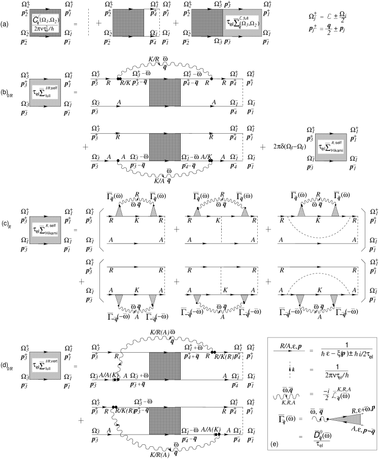
Figure 2: (a) Diagrammatic depiction of the Bethe-Salpeter equation Eq. (38) for the Cooperon $\bar{\cal C}_{\bm{q}}^{{\cal E}}(\Omega_{1},\Omega_{2})$. (b), (c) and (d): The contributions to the full self-energy ${\overline{\Sigma}}{}{}^{\cal E}_{{\bm{q}},\textrm{full}}(\Omega_{1},\Omega_{3})$ of Eq. (39a), namely (b): ${\overline{\Sigma}}{}{}^{{\cal E},I/R,\textrm{self}}_{{\bm{q}},{\bar{\bm{q}}},\textrm{full}}(\Omega_{1},\Omega_{3},{\bar{\omega}})$; (c) ${\overline{\Sigma}}{}{}^{{\cal E},R}_{{\bm{q}},{\bar{\bm{q}}},\textrm{Hikami}}(\Omega_{1},{\bar{\omega}})$ (which contributes to ${\overline{\Sigma}}{}{}^{R,\textrm{self}}_{\textrm{full}}$ only); and (d) ${\overline{\Sigma}}{}{}^{{\cal E},I/R,\textrm{vert}}_{{\bm{q}},{\bar{\bm{q}}},\textrm{full}}(\Omega_{1},\Omega_{3},{\bar{\omega}})$. The superscripts $I/R$ on ${\overline{\Sigma}}{}{}$ indicate which type of interaction propagator occurs: ${\overline{\Sigma}}{}{}^{I}$ (generated by $S_{I}$ in GZ’s approachGZ2 ; vonDelft04 ) contains ${\bar{\mathcal{L}}}^{K}$, together with ${\overline{\cal G}}{}^{R}$ and ${\overline{\cal G}}{}^{A}$ on the upper and lower contours, respectively; $\overline{\Sigma}^{R}$ (generated in GZ’s approach by $S_{R}$) contains a sum of two types of terms, featuring the combinations ${\bar{\mathcal{L}}}^{R}$ together with ${\overline{\cal G}}{}^{K}$ and ${\overline{\cal G}}{}^{A}$ on the upper and lower contours, or ${\bar{\mathcal{L}}}^{A}$ together with ${\overline{\cal G}}{}^{R}$ and ${\overline{\cal G}}{}^{K}$ on the upper and lower contours, respectively. The diagrams in (d) for ${\overline{\Sigma}}{}{}^{I/R,\textrm{vert}}_{\textrm{full}}$ occur both without and with bracketed labels for the interaction and electron propagators, e.g. $R$ or $(A)$ on ${\cal L}$, to distinguish contributions in which the electron Keldysh Green’s function occurs on the upper or lower electron line, respectively. The vertex to which the electron Keldysh Green’s function is attached is always indicated by a double dot (adopting a convention used in vonDelft04 ). (e) Diagrammatic conventions; the dressed interaction vertex is denoted by $\bar{\Gamma}_{\bar{q}}(\bar{\omega})=[{\overline{\cal D}}{}^{0}_{{\bar{\bm{q}}}}({\bar{\omega}})]/{\tau_{\textrm{el}}}$, where ${\overline{\cal D}}{}^{0}$ is the bare diffuson propagator.

This appendix diagrammatically specifies the Bethe-Salpeter equation governing the Cooperon, and gives explicit expressions for the full and bare Cooperon self-energies occuring therein.

A.1 Full Bethe-Salpeter equation

The diagrams specifying the Bethe-Salpeter equation for the full Cooperon, first written down in Ref. AAV, , are shown in Fig. 2. The feature that distinguishes “weak-localization” from “interaction” corrections to the conductivity is that for the former each current vertex is attached to a retarded and an advanced electron propagator, $G^{R}jG^{A}$, whereas for the latter, one or both current vertices are connected to two retarded or two advanced electron lines, $G^{R}jG^{R}$ or $G^{A}jG^{A}$. Hence, in setting up the Bethe-Salpeter equation, only those types of diagrams have been included for which the upper (or lower) lines entering and leaving the Cooperon are both retarded (or advanced) electron propagators. By adopting a pure ladder structure in Fig. 2(a), diagrams containing overlapping interaction lines have been dropped, but these are known GrilliSorella88 to be smaller than those included by at least a factor of $(k_{\textrm{F}}{l_{\textrm{el}}})^{-1}\ll 1$ (where ${l_{\textrm{el}}}$ is the mean free path).

Fig. 2(a) translates into the following equation:

$${1\over{\tau_{\textrm{el}}}}{\overline{\cal C}{}^{\cal E}_{\bm{q}}}(\Omega_{1},\Omega_{2}) = 2\pi\delta(\Omega_{12})+\left[{1\over{\tau_{\textrm{el}}}}-(E_{\bm{q}}-i\Omega_{1})\right]{\overline{\cal C}{}^{\cal E}_{\bm{q}}}(\Omega_{1},\Omega_{2})+\int(d\Omega_{3})\,{\overline{\Sigma}}{}{}^{\cal E}_{{\bm{q}},\textrm{full}}(\Omega_{1},\Omega_{3})\,{\overline{\cal C}{}^{\cal E}_{\bm{q}}}(\Omega_{3},\Omega_{2})\;.$$ (38)

This equation is equivalent to Eq. (II.2) of the main text.

The “Cooperon self-energy” ${\overline{\Sigma}}{}{}^{\cal E}_{{\bm{q}},\textrm{full}}$ occuring herein is defined by

$${\overline{\Sigma}}{}{}^{\cal E}_{{\bm{q}},\textrm{full}}(\Omega_{1},\Omega_{3}) = {1\over\hbar}\int(d{\bar{\bm{q}}})\int(d{\bar{\omega}})\left[{\overline{\Sigma}}{}{}^{{\cal E},I+R,\textrm{self}}_{{\bm{q}},{\bar{\bm{q}}},\textrm{full}}(\Omega_{1},\Omega_{3},{\bar{\omega}})+{\overline{\Sigma}}{}{}^{{\cal E},I+R,\textrm{vert}}_{{\bm{q}},{\bar{\bm{q}}},\textrm{full}}(\Omega_{1},\Omega_{3},{\bar{\omega}})\right]\,,\qquad\phantom{.}$$ (39a)

where the subscript $${\overline{\Sigma}}{}{}^{I+R} {\overline{\Sigma}}{}{}^{I}+{\overline{\Sigma}}{}{}^{R} {\overline{\Sigma}}{}{} \Omega_{j}^{\pm}\equiv{\cal E}\pm{\textstyle\frac{1}{2}}\Omega_{j}$$ indicates a sum , and the self-energy and vertex contributions to are given diagrammatically by Figs. 2(b) to 2(d). These lead to the following expressions (here ):

$${\overline{\Sigma}}{}{}^{{\cal E},I,\textrm{self}}_{{\bm{q}},{\bar{\bm{q}}},\textrm{full}}(\Omega_{1},\Omega_{3},{\bar{\omega}}) \equiv \phantom{-}{\textstyle\frac{1}{2}}i\bar{\cal L}{}^{K}_{\bar{\bm{q}}}({\bar{\omega}})\left[{\overline{\cal C}}{}^{{\cal E}-{1\over 2}{\bar{\omega}}}_{{\bm{q}}-{\bar{\bm{q}}}}(\Omega_{1}-{\bar{\omega}},\Omega_{3}-{\bar{\omega}})+{\overline{\cal C}}{}^{{\cal E}-{1\over 2}{\bar{\omega}}}_{{\bm{q}}-{\bar{\bm{q}}}}(\Omega_{1}+{\bar{\omega}},\Omega_{3}+{\bar{\omega}})\right]\;,\rule[-14.22636pt]{0.0pt}{0.0pt}$$ (39b)

$${\overline{\Sigma}}{}{}^{{\cal E},R,\textrm{self}}_{{\bm{q}},{\bar{\bm{q}}},\textrm{full}}(\Omega_{1},\Omega_{3},{\bar{\omega}}) \equiv \phantom{-}\tanh[(\Omega_{3}^{+}-{\bar{\omega}})/2T]\,{\textstyle\frac{1}{2}}i\bar{\cal L}{}^{R}_{\bar{\bm{q}}}({\bar{\omega}})\,{\overline{\cal C}}{}^{{\cal E}-{1\over 2}{\bar{\omega}}}_{{\bm{q}}-{\bar{\bm{q}}}}(\Omega_{1}-{\bar{\omega}},\Omega_{3}-{\bar{\omega}})$$

$$-\tanh[(\Omega_{1}^{-}-{\bar{\omega}})/2T]\,{\textstyle\frac{1}{2}}i\bar{\cal L}{}^{A}_{\bar{\bm{q}}}({\bar{\omega}})\,{\overline{\cal C}}{}^{{\cal E}-{1\over 2}{\bar{\omega}}}_{{\bm{q}}-{\bar{\bm{q}}}}(\Omega_{1}+{\bar{\omega}},\Omega_{3}+{\bar{\omega}})$$

$$+\;2\pi\delta(\Omega_{1}-\Omega_{3})\,{\overline{\Sigma}}{}{}^{{\cal E},R}_{{\bm{q}},{\bar{\bm{q}}},\textrm{Hikami}}(\Omega_{1},{\bar{\omega}})\;,\rule[-14.22636pt]{0.0pt}{0.0pt}$$

$${\overline{\Sigma}}{}{}^{{\cal E},R}_{{\bm{q}},{\bar{\bm{q}}},\textrm{Hikami}}(\Omega_{1},{\bar{\omega}}) \equiv \phantom{-}\tanh[(\Omega_{1}^{+}-{\bar{\omega}})/2T]\,{\textstyle\frac{1}{2}}i\bar{\cal L}{}^{R}_{\bar{\bm{q}}}({\bar{\omega}})\,\bigl{[}{\overline{\cal D}}{}^{0}_{\bar{\bm{q}}}({\bar{\omega}})\bigr{]}^{2}\left(\bigl{[}{\overline{\cal C}}{}^{0}_{{\bm{q}}}(\Omega_{1})\bigr{]}^{-1}+\bigl{[}{\overline{\cal D}}{}^{0}_{{\bar{\bm{q}}}}({\bar{\omega}})\bigr{]}^{-1}\right)\qquad\phantom{.}$$

$$-\tanh[(\Omega_{1}^{-}-{\bar{\omega}})/2T]\,{\textstyle\frac{1}{2}}i\bar{\cal L}{}^{A}_{\bar{\bm{q}}}({\bar{\omega}})\,\bigl{[}{\overline{\cal D}}{}^{0}_{-{\bar{\bm{q}}}}(-{\bar{\omega}})\bigr{]}^{2}\left(\bigl{[}{\overline{\cal C}}{}^{0}_{{\bm{q}}}(\Omega_{1})\bigr{]}^{-1}+\bigl{[}{\overline{\cal D}}{}^{0}_{{\bar{\bm{q}}}}(-{\bar{\omega}})\bigr{]}^{-1}\right),\rule[-14.22636pt]{0.0pt}{0.0pt}$$

$${\overline{\Sigma}}{}{}^{{\cal E},I,\textrm{vert}}_{{\bm{q}},{\bar{\bm{q}}},\textrm{full}}(\Omega_{1},\Omega_{3},{\bar{\omega}}) \equiv -{\textstyle\frac{1}{2}}i\bar{\cal L}{}^{K}_{\bar{\bm{q}}}({\bar{\omega}})\left[{\overline{\cal C}}{}^{{\cal E}+{1\over 2}{\bar{\omega}}}_{{\bm{q}}+{\bar{\bm{q}}}}(\Omega_{1}+{\bar{\omega}},\Omega_{3}-{\bar{\omega}})+{\overline{\cal C}}{}^{{\cal E}-{1\over 2}{\bar{\omega}}}_{{\bm{q}}-{\bar{\bm{q}}}}(\Omega_{1}+{\bar{\omega}},\Omega_{3}-{\bar{\omega}})\right]\;,\rule[-14.22636pt]{0.0pt}{0.0pt}$$ (39e)

$${\overline{\Sigma}}{}{}^{{\cal E},R,\textrm{vert}}_{{\bm{q}},{\bar{\bm{q}}},\textrm{full}}(\Omega_{1},\Omega_{3},{\bar{\omega}}) \equiv \phantom{-}\left[\tanh[\Omega_{1}^{+}/2T]\,\bar{\cal L}{}^{R}_{\bar{\bm{q}}}({\bar{\omega}})-\tanh[\Omega_{3}^{-}/2T]\,\bar{\cal L}{}^{A}_{\bar{\bm{q}}}({\bar{\omega}})\right]\!(-{\textstyle\frac{1}{2}}i)\,{\overline{\cal C}}{}^{{\cal E}+{1\over 2}{\bar{\omega}}}_{{\bm{q}}+{\bar{\bm{q}}}}(\Omega_{1}+{\bar{\omega}},\Omega_{3}-{\bar{\omega}})$$

$$+\left[\tanh[(\Omega_{3}^{+}-{\bar{\omega}})/2T]\,\bar{\cal L}{}^{R}_{\bar{\bm{q}}}({\bar{\omega}})-\tanh[(\Omega_{1}^{-}-{\bar{\omega}})/2T]\,\bar{\cal L}{}^{A}_{\bar{\bm{q}}}({\bar{\omega}})\right]\!(-{\textstyle\frac{1}{2}}i)\,{\overline{\cal C}}{}^{{\cal E}-{1\over 2}{\bar{\omega}}}_{{\bm{q}}-{\bar{\bm{q}}}}(\Omega_{1}+{\bar{\omega}},\Omega_{3}-{\bar{\omega}})\,.$$

The terms in Eq. (39), with their characteristic dependence on $\bigl{(}{\overline{\cal D}}{}^{0}\bigr{)}^{2}\bigl{[}\bigl{(}{\overline{\cal C}}{}^{0}\bigr{)}^{-1}+\bigl{(}{\overline{\cal D}}{}^{0}\bigr{)}^{-1}\bigr{]}$, stem from the Hikami-box contributions of Fig. 2(c). The ingredients entering the above equations are given by

$${{\bar{\cal L}{}^{K}_{\bar{\bm{q}}}({\bar{\omega}})}} = 2i\coth({\bar{\omega}}/2T)\,\textrm{Im}\bigl{[}\bar{\cal L}{}^{R}_{\bar{\bm{q}}}({\bar{\omega}})\bigr{]}\;,$$ (40a)

$${{\bar{\cal L}{}^{R}_{\bar{\bm{q}}}({\bar{\omega}})}} = [{{\bar{\cal L}{}^{A}_{\bar{\bm{q}}}({\bar{\omega}})}}]^{\ast}\simeq-{E^{0}_{\bar{\bm{q}}}-i{\bar{\omega}}\over 2\nu E_{\bar{\bm{q}}}^{0}}$$ (40b)

$${\overline{\cal C}}{}^{0}_{\bar{\bm{q}}}({\bar{\omega}}) = {1\over E_{\bar{\bm{q}}}-i{\bar{\omega}}}\;,\qquad{\overline{\cal D}}{}^{0}_{\bar{\bm{q}}}({\bar{\omega}})={1\over E_{\bar{\bm{q}}}^{0}-i{\bar{\omega}}}\;,\qquad\phantom{.}$$ (40c)

$$E^{0}_{\bar{\bm{q}}} \equiv D{\bar{\bm{q}}}^{2}\;,\qquad E_{\bar{\bm{q}}}\equiv D{\bar{\bm{q}}}^{2}+\gamma_{H}\;.$$ (40d)

In Eq. (40b) we have taken the usual “unitary limit”, which is relevant in the limit of small frequencies and momenta; the more general expression isAltshulerLarkin82

$${{\bar{\cal L}{}^{R}_{\bar{\bm{q}}}({\bar{\omega}})}} = -\;{E^{0}_{\bar{\bm{q}}}-i{\bar{\omega}}\over 2\nu E^{0}_{\bar{\bm{q}}}+(E^{0}_{\bar{\bm{q}}}-i{\bar{\omega}})/V^{(d)}_{\bar{\bm{q}}}}\;,$$ (41)

where $V^{(d)}_{\bar{\bm{q}}}=a^{3-d}\int d^{d}r\,e^{-i{\bar{\bm{q}}}r}(e^{2}/r)$ is the Fourier transform of the Coulomb potential in $d$ effective dimensions: $V^{(3)}_{\bar{\bm{q}}}={e^{2}\,4\pi/{\bar{\bm{q}}}^{2}}$, $V^{(2)}_{\bar{\bm{q}}}={a\,e^{2}\,2\pi/|{\bar{\bm{q}}}|}$, and $V^{(1)}_{\bar{\bm{q}}}=a^{2}e^{2}\ln({\bar{\bm{q}}}^{2}a^{2})$.

A.2 Bare Self-Energies

Since the self-energies ${\overline{\Sigma}}{}{}_{\textrm{full}}$ of Eqs. (39) are proportional to the Cooperon ${\overline{\cal C}}{}$, the Bethe-Salpeter equation (II.2) is non-linear in ${\overline{\cal C}}{}$. Solving it in its full glory thus seems hardly feasible. Thus, we shall “linearize” it by making the replacement ${\overline{\cal C}}{}^{\cal E}_{{\bm{q}}}(\Omega_{1},\Omega_{3})\to 2\pi\delta(\Omega_{13})\,{\overline{\cal C}}{}^{0}_{\bm{q}}(\Omega_{1})$ for every occurence of the full Cooperon in the self-energy terms. The resulting bare self-energies can be written in the form

$${\overline{\Sigma}}{}{}^{\cal E}_{{\bm{q}},\textrm{bare}}(\Omega_{1},\Omega_{4}) = {1\over\hbar}\int(d{\bar{\bm{q}}})\int(d{\bar{\omega}})\,2\pi\left[\delta(\Omega_{14})\,{\overline{\Sigma}}{}{}^{{\cal E}+{1\over 2}\Omega_{4},\textrm{self}}_{{\bm{q}},{\bar{\bm{q}}},\textrm{bare}}(\widetilde{\Omega}_{14},{\bar{\omega}})\,+\,\delta(\Omega_{14}+2{\bar{\omega}})\,{\overline{\Sigma}}{}{}^{{\cal E}+{1\over 2}\Omega_{4},\textrm{vert}}_{{\bm{q}},{\bar{\bm{q}}},\textrm{bare}}(\widetilde{\Omega}_{14},{\bar{\omega}})\right],\qquad\phantom{.}$$ (42a)

where $$\Omega_{14}\equiv\Omega_{1}-\Omega_{4} \widetilde{\Omega}_{14}\equiv{\textstyle\frac{1}{2}}(\Omega_{1}+\Omega_{4})$$ and , with the following ingredients:

$${\overline{\Sigma}}{}{}^{{\cal E},\textrm{self}}_{{\bm{q}},{\bar{\bm{q}}},\textrm{bare}}(\omega,{\bar{\omega}}) = \left[{\overline{\Sigma}}{}{}^{{\cal E},\textrm{self},\textrm{dec}}_{{\bm{q}},{\bar{\bm{q}}},\textrm{bare}}+{\overline{\Sigma}}{}{}^{{\cal E},\textrm{self},Z}_{{\bm{q}},{\bar{\bm{q}}},\textrm{bare}}\right](\omega,{\bar{\omega}})\;,\rule[-14.22636pt]{0.0pt}{0.0pt}$$ (42b)

$${\overline{\Sigma}}{}{}^{{\cal E},\textrm{self},\textrm{dec}}_{{\bm{q}},{\bar{\bm{q}}},\textrm{bare}}(\omega,{\bar{\omega}}) \equiv -\left[{\overline{\cal C}}{}^{0}_{{\bm{q}}-{\bar{\bm{q}}}}(\omega-{\bar{\omega}})+{\overline{\cal C}}{}^{0}_{{\bm{q}}-{\bar{\bm{q}}}}(\omega+{\bar{\omega}})\right]\bar{\cal L}{}^{\textrm{dec}}_{{\cal E}\omega,{\bar{\bm{q}}}}({\bar{\omega}})\;,\rule[-14.22636pt]{0.0pt}{0.0pt}$$ (42c)

$${\overline{\Sigma}}{}{}^{{\cal E},\textrm{self},Z}_{{\bm{q}},{\bar{\bm{q}}},\textrm{bare}}(\omega,{\bar{\omega}}) \equiv \phantom{+}\tanh[({\cal E}-{\bar{\omega}})/2T]\,{\textstyle\frac{1}{2}}i\bar{\cal L}{}^{R}_{\bar{\bm{q}}}({\bar{\omega}})\left[\left[{\overline{\cal D}}{}^{0}_{\bar{\bm{q}}}({\bar{\omega}})\right]^{2}\Bigl{(}\bigl{[}{\overline{\cal C}}{}^{0}_{{\bm{q}}}(\omega)\bigr{]}^{-1}+\bigl{[}{\overline{\cal D}}{}^{0}_{{\bar{\bm{q}}}}({\bar{\omega}})\bigr{]}^{-1}\Bigr{)}-{\overline{\cal C}}{}^{0}_{{\bm{q}}-{\bar{\bm{q}}}}(\omega+{\bar{\omega}})\right]$$

$$-\tanh[({\cal E}-{\bar{\omega}}-\omega)/2T]\,{\textstyle\frac{1}{2}}i\bar{\cal L}{}^{A}_{\bar{\bm{q}}}({\bar{\omega}})\left[\left[{\overline{\cal D}}{}^{0}_{\bar{\bm{q}}}(-{\bar{\omega}})\right]^{2}\Bigl{(}\bigl{[}{\overline{\cal C}}{}^{0}_{{\bm{q}}}(\omega)\bigr{]}^{-1}+\bigl{[}{\overline{\cal D}}{}^{0}_{{\bar{\bm{q}}}}(-{\bar{\omega}})\bigr{]}^{-1}\Bigr{)}-{\overline{\cal C}}{}^{0}_{{\bm{q}}-{\bar{\bm{q}}}}(\omega-{\bar{\omega}})\right]\;,\qquad\rule[-14.22636pt]{0.0pt}{0.0pt}$$

$${\overline{\Sigma}}{}{}_{{\bm{q}},{\bar{\bm{q}}},\textrm{bare}}^{{\cal E},\textrm{vert}}(\omega,{\bar{\omega}}) \equiv 2{\overline{\cal C}}{}^{0}_{{\bm{q}}-{\bar{\bm{q}}}}(\omega)\,\bar{\cal L}{}^{\textrm{dec}}_{{\cal E}\omega,{\bar{\bm{q}}}}({\bar{\omega}})\;,\rule[-14.22636pt]{0.0pt}{0.0pt}$$ (42e)

$$\bar{\cal L}{}^{\textrm{dec}}_{{\cal E}\omega,{\bar{\bm{q}}}}({\bar{\omega}}) \equiv \coth[{\bar{\omega}}/2T]\,\textrm{Im}\bigl{[}\bar{\cal L}{}^{R}_{\bar{\bm{q}}}({\bar{\omega}})\bigr{]}-\tanh[({\cal E}-{\bar{\omega}})/2T]\,{\textstyle\frac{1}{2}}i\bar{\cal L}{}^{R}_{\bar{\bm{q}}}({\bar{\omega}})+\tanh[({\cal E}-{\bar{\omega}}-\omega)/2T]\,{\textstyle\frac{1}{2}}i\bar{\cal L}{}^{A}_{\bar{\bm{q}}}({\bar{\omega}})\;.\qquad$$ (42f)

We have split the self-energy contribution [stemming from Eqs. (39b) plus (39)] into two terms, ${\overline{\Sigma}}{}{}^{\textrm{self},\textrm{dec}}_{\textrm{bare}}+{\overline{\Sigma}}{}{}^{\textrm{self},Z}_{\textrm{bare}}$, chosen such that the Hikami-box contributions are fully contained in ${\overline{\Sigma}}{}{}^{\textrm{self},Z}_{\textrm{bare}}$, and that both $\Sigma^{\textrm{self},\textrm{dec}}_{\textrm{bare}}$ and ${\overline{\Sigma}}{}{}^{\textrm{vert}}_{\textrm{bare}}$ are proportional to the same combination of propagators, $\bar{\cal L}{}^{\textrm{dec}}$ [Eq. (42f)], a feature that considerably simplifies the analysis in the main text. To achieve this, the terms in Eq. (42) that are proportional to $\tanh\cdot\,{\overline{\cal C}}{}^{0}_{{\bm{q}}-{\bar{\bm{q}}}}(\omega\pm{\bar{\omega}})$ were added in Eq. (42c) and subtracted in (42), respectively. This addition-subtraction trick amounts to ”replacing” the Hikami-box contribution to $\Sigma^{\textrm{self},\textrm{dec}}_{\textrm{bare}}$ by “replacement terms” [those added to Eq. (42c)] that (i) have a simpler, more convenient structure (since proportional to ${\overline{\cal C}}{}^{0}$ instead of $\bigl{(}{\overline{\cal D}}{}^{0}\bigr{)}^{2}\bigl{[}\bigl{(}{\overline{\cal C}}{}^{0}\bigr{)}^{-1}+\bigl{(}{\overline{\cal D}}{}^{0}\bigr{)}^{-1}\bigr{]}$), but (ii) nevertheless have the same leading infrared and ultraviolet behavior, in the sense that the difference between the Hikami-box and the replacement terms, namely ${\overline{\Sigma}}{}{}^{\textrm{self},Z}$, generates only subleading contributions to the long-time behavior of the Cooperon (as explained below). The leading contribution comes from ${\overline{\Sigma}}{}{}^{\textrm{self},\textrm{dec}}$ and ${\overline{\Sigma}}{}{}^{\textrm{vert}}$, because both are proportional to the effective propagator $\bar{\cal L}{}^{\textrm{dec}}_{{\cal E}\omega,{\bar{\bm{q}}}}({\bar{\omega}})$, whose $\coth[{\bar{\omega}}/2T]$ term at small frequencies ${\bar{\omega}}$ makes the dominant contribution [in contrast, ${\overline{\Sigma}}{}{}^{\textrm{self},Z}$ lacks such a term].

Although the dominant contribution comes from low frequencies, ${\overline{\Sigma}}{}{}^{\textrm{self},\textrm{dec}}+{\overline{\Sigma}}{}{}^{\textrm{vert}}$ contain no infrared divergence, since for ${\bar{\omega}}\to 0$, their contributions cancel each other, as is clear directly from Eqs. (42c) and (42e) (or by inserting them into Eqs. (43) and (43) below, or Eq. (29) of the main text). Moroever, the dominant contribution from ${\overline{\Sigma}}{}{}^{\textrm{self},\textrm{dec}}+{\overline{\Sigma}}{}{}^{\textrm{vert}}$ also contains no ultraviolet divergencies, since the effective propagator $\bar{\cal L}{}^{\textrm{dec}}_{{\cal E}\omega,{\bar{\bm{q}}}}({\bar{\omega}})$ evidently vanishes exponentially in the limit ${\bar{\omega}}\gg{\cal E},T$, hence the $\int(d{\bar{\omega}})$ integrals over both ${\overline{\Sigma}}{}{}^{{\cal E},\textrm{self},\textrm{dec}}_{{\bm{q}},{\bar{\bm{q}}},\textrm{bare}}(\omega,{\bar{\omega}})$ and ${\overline{\Sigma}}{}{}^{{\cal E},\textrm{vert}}_{{\bm{q}},{\bar{\bm{q}}},\textrm{bare}}(\omega,{\bar{\omega}})$ are separately free from ultraviolet divergencies.

Concerning the contribution from ${\overline{\Sigma}}{}{}^{\textrm{self},Z}$, there are several ways to convince oneself that its contribution to the Cooperon decay function $F(t)$ is subleading. Firstly, an explicit calculation, performed in Appendix C.2, shows that its contribution to $\tilde{C}^{(1)\varepsilon}$, the first-order expansion of the Cooperon in powers of the interaction propagator, depends much more weakly on propagation time $t$ than that from ${\overline{\Sigma}}{}{}^{\textrm{self},\textrm{dec}}+{\overline{\Sigma}}{}{}^{\textrm{vert}}$; for example, for quasi 1-dimensions it scales with $t^{-1/2}$ [cf. Eq. (66)], compared to the $t^{1}$ of the leading terms ${\tilde{C}}^{0}(0,t)\tilde{F}^{\varepsilon}(t)$.

An alternative, and more simple, argument goes as follows: according to the short-cut “self-energy-diagrams-only” approach of Section II.3, the decoherence rate is given by $\gamma_{\varepsilon,0}^{\varphi,\textrm{self}}$ of Eq. (12b) [see also (14b)], for which we have to set $E_{\bm{q}}=i\omega$ and take $q\to 0$. Now, in this limit ${\overline{\Sigma}}{}{}^{\textrm{self},Z}_{\varepsilon,{\bm{q}}}(\omega)$ vanishes identically, regardless of the form of the interaction propagator ${{\bar{\cal L}{}^{R}_{\bar{\bm{q}}}({\bar{\omega}})}}$, and hence does not contribute to $\gamma_{\varepsilon,0}^{\varphi,\textrm{self}}$ at all. Actually, an even stronger statement can be made if the general form (41) for the interaction propagator is specialized to the the so-called “unitary limit” of Eq. (40b) (as is usually done anyway). In that case, both the Hikami-box terms and the “replacement terms” separately vanish in the limit $E_{\bm{q}}=i\omega$ and $q\to 0$. Thus, for the “unitary limit” of the interaction propagator, Hikami-box contributions actually do not contribute to the decoherence rate at allvonDelft04 . It is for this (somewhat fortuitous) reason that the influence functional theory of decoherence developed in Ref. vonDelft04, was able to correctly obtain the Cooperon decay function, despite of the fact that it did not include any Hikami-box contributions.

A.3 Expansion to 2nd order in the interaction

The object needed on the right-hand side of Eq. (5d) for $\tilde{C}^{\varepsilon}(r_{12},t_{1},t_{2})$ is ${\overline{\cal C}}{}^{\varepsilon-{1\over 2}\Omega_{2}}_{{\bm{q}}}(\Omega_{1},\Omega_{2})$, which is determined by the Bethe-Salpeter equation Eq. (II.2), with ${\cal E}=\varepsilon-{\textstyle\frac{1}{2}}\Omega_{2}$ (with $\omega_{0}=0$ here). It is instructive to consider the first few terms that are obtained upon iterating this equation, while using the bare self-energies of Eq. (42a). (Of course, as soon as we go beyond first order, we should not use the bare self-energy, but the full one, which should be calculated iteratively order by order, too; we shall refrain from doing so here, since our intention is merely to illustrate the general structure of the terms arising in second and higher orders, not to evaluate them explicitly.) ${\overline{\cal C}}{}^{\varepsilon-{1\over 2}\Omega_{2}}_{{\bm{q}}}(\Omega_{1},\Omega_{2})={\overline{\cal C}}{}^{(0)}+{\overline{\cal C}}{}^{(1)}+{\overline{\cal C}}{}^{(2)}$, and evaluating the result for $\Omega_{1,2}=\omega\mp{\widetilde{\omega}}$, we obtain:

$${\overline{\cal C}}{}^{(0)} = {\overline{\cal C}}{}^{0}_{\bm{q}}(\omega)\,\delta(2{\widetilde{\omega}})\;,$$ (43a)

$${\overline{\cal C}}{}^{(1)} = {1\over\hbar}\int(d{\bar{\bm{q}}}_{1})(d{\bar{\omega}}_{1})\Biggl{\{}\delta(2{\widetilde{\omega}})\,{\overline{\cal C}}{}^{0}_{\bm{q}}(\omega)\,{\overline{\Sigma}}{}{}^{\varepsilon,\textrm{self}}_{{\bm{q}},{\bar{\bm{q}}}_{1},\textrm{bare}}(\omega,{\bar{\omega}}_{1})\,{\overline{\cal C}}{}^{0}_{\bm{q}}(\omega)\,\Biggr{.}$$

$$\qquad\Biggl{.}+\,\delta(2{\widetilde{\omega}}-2{\bar{\omega}}_{1})\,{\overline{\cal C}}{}^{0}_{\bm{q}}(\omega-{\bar{\omega}}_{1})\,{\overline{\Sigma}}{}{}^{{\varepsilon},\textrm{vert}}_{{\bm{q}},{\bar{\bm{q}}}_{1},\textrm{bare}}(\omega,{\bar{\omega}}_{1})\,{\overline{\cal C}}{}^{0}_{\bm{q}}(\omega+{\bar{\omega}}_{1})\Biggr{\}}\;,$$

$${\overline{\cal C}}{}^{(2)} = {1\over\hbar^{2}}\int(d{\bar{\bm{q}}}_{1})(d{\bar{\omega}}_{1})(d{\bar{\bm{q}}}_{2})(d{\bar{\omega}}_{2})\Biggl{\{}\delta(2{\widetilde{\omega}})\,{\overline{\cal C}}{}^{0}_{\bm{q}}(\omega)\,{\overline{\Sigma}}{}{}^{{\varepsilon},\textrm{self}}_{{\bm{q}},{\bar{\bm{q}}}_{1},\textrm{bare}}(\omega,{\bar{\omega}}_{1})\,{\overline{\cal C}}{}^{0}_{\bm{q}}(\omega)\,{\overline{\Sigma}}{}{}^{\varepsilon,\textrm{self}}_{{\bm{q}},{\bar{\bm{q}}}_{2},\textrm{bare}}(\omega,{\bar{\omega}}_{2})\,{\overline{\cal C}}{}^{0}_{\bm{q}}(\omega)\Biggr{.}\qquad\phantom{.}$$

$$+\,\delta(2{\widetilde{\omega}}-2{\bar{\omega}}_{1})\,{\overline{\cal C}}{}^{0}_{\bm{q}}(\omega-{\bar{\omega}}_{1})\,{\overline{\Sigma}}{}{}^{\varepsilon,\textrm{vert}}_{{\bm{q}},{\bar{\bm{q}}}_{1},\textrm{bare}}(\omega,{\bar{\omega}}_{1})\,{\overline{\cal C}}{}^{0}_{\bm{q}}(\omega+{\bar{\omega}}_{1})\,{\overline{\Sigma}}{}{}^{\varepsilon,\textrm{self}}_{{\bm{q}},{\bar{\bm{q}}}_{2},\textrm{bare}}(\omega+{\bar{\omega}}_{1},{\bar{\omega}}_{2})\,{\overline{\cal C}}{}^{0}_{\bm{q}}(\omega+{\bar{\omega}}_{1})\,\rule{0.0pt}{14.22636pt}$$

$$+\,\delta(2{\widetilde{\omega}}-2{\bar{\omega}}_{2})\,{\overline{\cal C}}{}^{0}_{\bm{q}}(\omega-{\bar{\omega}}_{2})\,{\overline{\Sigma}}{}{}^{\varepsilon-{\bar{\omega}}_{2},\textrm{self}}_{{\bm{q}},{\bar{\bm{q}}}_{1},\textrm{bare}}(\omega-{\bar{\omega}}_{2},{\bar{\omega}}_{1})\,{\overline{\cal C}}{}^{0}_{\bm{q}}(\omega-{\bar{\omega}}_{2})\,{\overline{\Sigma}}{}{}^{\varepsilon,\textrm{vert}}_{{\bm{q}},{\bar{\bm{q}}}_{2},\textrm{bare}}(\omega,{\bar{\omega}}_{2})\,{\overline{\cal C}}{}^{0}_{\bm{q}}(\omega+{\bar{\omega}}_{2})\,\rule{0.0pt}{19.91692pt}\qquad\phantom{.}$$

$$+\,\delta(2{\widetilde{\omega}}-2{\bar{\omega}}_{1}-2{\bar{\omega}}_{2})\,{\overline{\cal C}}{}^{0}_{\bm{q}}(\omega-{\bar{\omega}}_{1}-{\bar{\omega}}_{2})\,{\overline{\Sigma}}{}{}^{\varepsilon-{\bar{\omega}}_{2},\textrm{vert}}_{{\bm{q}},{\bar{\bm{q}}}_{1},\textrm{bare}}(\omega-{\bar{\omega}}_{2},{\bar{\omega}}_{1})\,{\overline{\cal C}}{}^{0}_{\bm{q}}(\omega+{\bar{\omega}}_{1}-{\bar{\omega}}_{2})\,\rule{0.0pt}{19.91692pt}$$

$$\Biggl{.}\qquad\times{\overline{\Sigma}}{}{}^{\varepsilon,\textrm{vert}}_{{\bm{q}},{\bar{\bm{q}}}_{2},\textrm{bare}}(\omega+{\bar{\omega}}_{1},{\bar{\omega}}_{2})\,{\overline{\cal C}}{}^{0}_{\bm{q}}(\omega+{\bar{\omega}}_{1}+{\bar{\omega}}_{2})\,\Biggr{\}}$$

These expressions are useful for illustrating two important general points. Firstly, the expansion (43) allows us to confirm explicitly a fact well-known to practitioners of diagrammatic perturbation theory, namely that the calculation of the Cooperon is free of ultraviolet divergencies. This fact was implicitly challenged by GZ, whose conclusion of a finite decoherence rate at zero temperature stems from the occurence of an ultraviolet divergence in their expression for the decoherence rate. (GZ’s expression for $\gamma^{\textrm{GZ}}$ for $d=1$ [Eq. (76) for LABEL:GZ2] has the form of our Eq. (17), but without the $\tanh$-term, whence they introduced an upper cut ${\bar{\omega}}_{\textrm{max}}\simeq 1/{\tau_{\textrm{el}}}$ in the frequency integral there; the relation of their work to ours is discussed in more detail in Paper I, Sec. LABEL:sec:GZcomparison.) However, it is straightforward to check [using Eqs. (42)] that the perturbative expansion (43) generates no ultraviolet divergencies when used to calculate that version of the Cooperon governing the conductivity, namely $\tilde{\cal C}_{\textrm{cond}}^{\varepsilon,\omega_{0}}$ of Eq. (3b): the reason is simply that both ${\overline{\Sigma}}{}{}^{\textrm{self},\textrm{dec}}$ and ${\overline{\Sigma}}{}{}^{\textrm{vert}}$ are proportional to the propagator $\bar{\cal L}{}^{\textrm{dec}}_{{\cal E}\omega,{\bar{\bm{q}}}}({\bar{\omega}})$, which serves as ultraviolet cutoff at ${\bar{\omega}}\simeq T$. [The contribution from ${\overline{\Sigma}}{}{}^{\textrm{self},Z}$ is subdominant, as mentioned above; in fact, ${\overline{\Sigma}}{}{}^{{\cal E},\textrm{self},Z}_{{\bm{q}},{\bar{\bm{q}}},\textrm{bare}}(\omega,{\bar{\omega}})\to 0$ in the limit of large ${\bar{\omega}}$, and its leading nonzero contribution turns out to be UV-convergent if the general expression (41) is used for the interaction propagator, instead of its small-frequency approximation (40b).]

Secondly, we note that the frequency arguments ${\bar{\omega}}_{i}$ get more and more “entangled” from order to order in perturbation theory, i.e., they occur in increasingly complicated combinations as arguments of ${\overline{\Sigma}}{}{}^{\textrm{self}/\textrm{vert}}$, because the vertex diagrams cause a proliferation of frequency transfers between the upper and lower Cooperon lines. In $n$-th order, the generic structure will be

$${\overline{\cal C}}{}^{(n)}\sim\prod_{j=1}^{n}\int(d\bar{\omega}_{j}){\overline{\cal C}}{}^{(0)}(\cdot){\overline{\Sigma}}{}(\cdot,\bar{\omega}_{1})\dots\overline{\Sigma}{}(\cdot,\bar{\omega}_{1}){\overline{\cal C}}{}^{(0)}(\cdot),\quad\phantom{.}$$ (44)

where $(\cdot)$ stands for combinations of frequency arguments that can contain any number of $\bar{\omega}_{j}$’s. Due to this entanglement, a direct solution of the Bethe-Salpeter equation (II.2) is intractable, and further approximations are needed, that somehow “factorize” the entangled frequency integrals and thereby truncate the proliferation of frequency transfers.

A natural truncation scheme would be to retain the frequency transfer ${\bar{\omega}}_{j}$ generated by a given vertex line only in the corresponding vertex function ${\overline{\Sigma}}{}^{\varepsilon,\textrm{vert}}_{{\bm{q}},{\bar{\bm{q}}}_{j}}(\omega,{\bar{\omega}}_{j})$, and to neglect it everywhere else in the diagram. As a result, it would again become possible to associate a definite frequency label with the upper and lower electron lines of the Cooperon (say $\varepsilon$ and $\varepsilon-\omega$). In fact, such an approximation was in effect adopted in the integral functional approach of Ref. vonDelft04, and paper I (which both implicitly also took the “long-time limit” $\omega=0$, for reasons explained in the last paragraph of Sec. LABEL:sec:Simplified-influence-action of paper I). Such a procedure can be justified as follows: The only reason for incorporating the (frequency-proliferating) vertex terms in the first place, is to cure the infrared divergencies arising from the self-energy terms, which are thereby cut off at frequencies $\bar{\omega}\simeq 1/t$ [this is perhaps seen most clearly from the $\bigl{[}1-\sin(\bar{\omega}t)/(\bar{\omega}t)\bigr{]}$ factor in Eq. (I.LABEL:eq:simpleFdurw)]. For larger frequencies $\bar{\omega}\gtrsim 1/t$, the contribution of vertex diagrams is always subleading compared to that of the matching self-energy diagrams, and hence can be neglected without affecting the leading behavior of the decay function $\tilde{F}_{d}(t)$. Thus, it suffices to treat the ${\bar{\omega}}_{j}$-dependence associated with the frequency transfer between the forward and backward contours in the vertex part of ${\overline{\Sigma}}{}(\cdot,\bar{\omega}_{j})$ explicitly only within this particular factor [i.e. in the interaction propagator, associated $\coth+\tanh$ functions, and associated Cooperons of ${\overline{\Sigma}}{}(\cdot,\bar{\omega}_{j})$]. Since the accociated contribution is dominated by frequencies $\bar{\omega}\simeq 1/t$, which are small in the long-time limit, all other factors ${\overline{\cal C}}{}(\cdot)$ and ${\overline{\Sigma}}{}(\cdot,\bar{\omega}_{i\neq j})$ of the diagram to which this ${\bar{\omega}}_{j}$-dependence has propagated may be Taylor-expanded in ${\bar{\omega}}_{j}$. Moreover, only the zeroth-order terms of this Taylor expansion need to be retained, since the others contain higher powers of ${\bar{\omega}}_{j}\sim 1/t$, and hence produce contributions with a subleading time dependence [as illustrated in App. C.1, where such an expansion is carried out explicitly in a very similar context].

Having clarified that a truncation scheme is justified in principle in the long-time limit, we have to implement one in practice, in such a way that the leading terms are not affected. In the present context, the simplest version of such a truncation scheme would be to replace the $\delta(\Omega_{14}+2{\bar{\omega}})$ in Eq. (42a) by $\delta(\Omega_{14})$, thereby rendering the entire equation for ${\overline{\Sigma}}{}{}^{\cal E}_{{\bm{q}},\textrm{bare}}(\Omega_{1},\Omega_{4})$ proportional to $\delta(\Omega_{14})$. As a result, the arguments of the “self-energy-diagram-only” discussion in Section II.3 would apply: the Bethe-Salpter equation could then be simplified to a Dyson-type equation, whose self-energy would be given by an expression analogous to Eq. (11), but now including a vertex contribution:

$${\overline{\Sigma}}{}{}^{\textrm{s+v}}_{\varepsilon,{\bm{q}}}(\omega)\equiv{1\over\hbar}\int(d{\bar{\omega}})(d{\bar{\bm{q}}})\,\left[{\overline{\Sigma}}{}{}^{\varepsilon,\textrm{self}}_{{\bm{q}},{\bar{\bm{q}}},\textrm{bare}}+{\overline{\Sigma}}{}{}^{\varepsilon,\textrm{vert}}_{{\bm{q}},{\bar{\bm{q}}},\textrm{bare}}\right](\omega,{\bar{\omega}})\,.$$

However, note that it would now not be possible to calculate the decoherence rate $\gamma_{\varepsilon,0}^{\varphi,\textrm{self}}$ according to Eq. (12b) by setting $E_{\bm{q}}=i\omega$ and ${\bm{q}}=0$ in ${\overline{\Sigma}}{}{}^{\textrm{s+v}}_{\varepsilon,{\bm{q}}}(\omega)$, because the factor ${\overline{\cal C}}{}^{0}_{{\bm{q}}-{\bar{\bm{q}}}}(\omega)$ contained in ${\overline{\Sigma}}{}{}^{\varepsilon,\textrm{vert}}_{{\bm{q}},{\bar{\bm{q}}},\textrm{bare}}(\omega,{\bar{\omega}})$ would then yield an infrared divergence for ${\bar{\bm{q}}}\to 0$.

To avoid this problem, a version of the calculation has to be found in which the condition $E_{\bm{q}}=i\omega$ is avoided, and the variables ${\bm{q}}$ and $\omega$ are integrated over instead. In Section III of the main text this is achieved by transcribing the Bethe-Salpeter equation to the position-time domain, and solving it with an exponential Ansatz, $\tilde{C}({\bm{r}}_{12};t_{1},t_{2})\simeq\tilde{C}^{0}e^{[\tilde{C}^{(1)}/\tilde{C}^{0}]}$, where $\tilde{C}^{(1)}({\bm{r}}_{12};t_{1},t_{2})$ is an appropriately Fourier-transformed version of Eq. (43) involving $\int(dq)(dw)$ integrals, precisely as desired. This is a factorization approximation, in the sense that a proliferation of entangled frequencies is avoided by approximating the $n$-th order contribution to the Cooperon by $\tilde{C}^{(n)}\simeq{1\over n!}[\tilde{C}^{(1)}]^{n}/[\tilde{C}^{0}]^{n-1}$.

Note that in this scheme, the frequency transfer between forward and backward lines generated by the vertex terms is treated exactly in the first order terms needed for $C^{(1)}$; the factorization approximation sets in only in second and higher orders. Treating the first order terms exactly is the best one can do in our reexponentiation-of-$C^{(1)}$ scheme, since in the latter, an accurate treatment of effects occuring only in second or higher order is beyond the accuracy of the method. The accumulation of energy transfers is such an effect, but fortunately it produces corrections that are only subleading in time, as argued above.

Appendix B The Bethe-Salpeter equation yields the exact Cooperon in the classical limit

In general, solving a Bethe-Salpeter equation starting from a self-energy calculated only to lowest order in the interaction does not provide the exact solution of the initial problem. This remains true even when the self-energy is treated self-consistently (i.e. inserting the full propagators into the diagram for $\Sigma$, as we have done for $\Sigma_{\rm full}$). Nevertheless, in the following we shall demonstrate that for $d=1$ and classical white Nyquist noise, the exact solution of the Bethe-Salpeter equation (22) fully reproduces the exact results for the Cooperon derived by AAK AAK , implying that our Bethe-Salpeter equation itself is exact for this type of noise. The reason for this may be traced back to the special properties of the white Nyquist noise interaction propagator, as will be explained below. Thus, non-exact results obtained from our Bethe-Salpeter equation for $d=1$ and white noise are entirely due to approximations involved in constructing a solution, such as the “re-exponentation” of the first order result. (Actually, the deviations resulting from the latter approximation produces are quantitatively rather small, as demonstrated in Paper I [Section LABEL:sec:1Dcompare].)

We start from the Bethe-Salpeter equation, Eq. (22), using the full (not bare!) self-energy $\tilde{\Sigma}_{\textrm{full}}$, given by Eqs. (III.1) and (39). The latter simplifies considerably for classical white Nyquist noise, described by setting $\bar{\cal L}{}^{R/A}_{\bar{q}}({\bar{\omega}})\mapsto 0$ and $-{\textstyle\frac{1}{2}}i\bar{\cal L}{}^{K}_{\bar{\bm{q}}}({\bar{\omega}})\mapsto\bar{\cal L}{}^{\textrm{cl}}_{\bar{q}}\equiv T/(\nu D{\bar{q}}^{2})$. The first replacement implies that the self energy diagrams, and hence also the Cooperon ${\overline{\cal C}}{}^{\cal E}_{{\bm{q}}}(\Omega_{1},\Omega_{2})$, no longer depend on ${\cal E}$, so that this argument will be dropped henceforth. The second replacement results in an interaction propagator that is not only independent of $\varepsilon$, $\omega$ but also of ${\bar{\omega}}$, i.e. white in frequency transfers, implying that it becomes a $\delta$-function in the time domain. The resulting self energy has the form

$$\tilde{\Sigma}^{\varepsilon,t^{\prime}_{4}}_{\textrm{full}}({{\bm{r}}_{14}};t_{1},t_{4})=\widetilde{W}^{\prime}_{\textrm{cl}}(r_{14})\bigl{[}\delta(\widetilde{t}_{14})-\delta(t_{14})\bigr{]}\delta(t_{4^{\prime}}),\quad\phantom{.}$$ (45)

where $\widetilde{W}^{\prime}_{\textrm{cl}}(r_{14})={2\over\hbar}\int(d{\bar{q}})\bar{\cal L}{}^{\textrm{cl}}_{\bar{\bm{q}}}e^{i{\bar{q}}r_{14}}$. This is ultraviolet convergent only for $d=1$, to which we henceforth restrict our attention, but then $\widetilde{W}^{\prime}_{\textrm{cl}}(r_{14})$ is infrared divergent. However, when Eq. (45) is inserted into Eq. (22), this divergence can be arranged to cancel between the two terms of Eq. (45): its second term, which stems from $\Sigma^{\textrm{self}}$, produces [using ${\tilde{C}}(r_{14};t_{1},t_{1})=\delta(r_{14})$] a contribution $-\widetilde{W}^{\prime}_{\textrm{cl}}(0)\,{\tilde{C}}(r_{12};t_{1},t_{2})$, which can be rewritten as $-\widetilde{W}^{\prime}_{\textrm{cl}}(0)\int d{\bm{r}}_{4}{\tilde{C}}(r_{14};t_{1},-t_{1}){\tilde{C}}(r_{42};-t_{1},t_{2})$, so that it takes a form similar to that resulting from the first (vertex) term of Eq. (45). Thus, the Bethe-Salpeter equation (22) can be written as

$$\bigl{(}-D\nabla^{2}_{{\bm{r}}_{1}}+\partial_{t_{1}}+{\gamma_{H}}\bigr{)}\,{\tilde{C}}(r_{12};t_{1},t_{2})=\delta({\bm{r}}_{12})\,\delta(t_{12})+$$

$$\int d{\bm{r}}_{4}\widetilde{W}_{\textrm{cl}}(r_{14})\,{\tilde{C}}(r_{14};t_{1},-t_{1}){\tilde{C}}(r_{42};-t_{1},t_{2})\;,$$ (46)

where the kernel $\widetilde{W}_{\textrm{cl}}(r_{14})=\widetilde{W}^{\prime}_{\textrm{cl}}(r_{14})-\widetilde{W}^{\prime}_{\textrm{cl}}(0)$ is free of infrared problems:

$$\widetilde{W}_{\textrm{cl}}(r)=\int{d{\bar{q}}\over 2\pi}{4e^{2}T\over\hbar\sigma_{1}}{e^{i{\bar{q}}r}-1\over{\bar{q}}^{2}}\,.$$ (47)

(Here $\sigma_{1}=a^{2}2\nu e^{2}D$ is the inverse resistance per length of a quasi 1-dimensional wire of cross section $a^{2}$.)

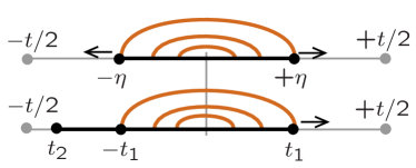
Figure 3: Schematic illustration of the time-evolution in the differential equation for the Cooperon: AAK’s scheme (top) evolves both endpoints symmetrically, while the full Bethe-Salpeter equation (bottom) contains two Cooperons, describing propagation in the intervals $(t_{2},-t_{1})$ and $(-t_{1},t_{1})$. Curved lines represent interaction propagators.

Eq. (46) is solved by the following path integral:

$${\tilde{C}}(r_{12};t_{1},t_{2})=\theta(t_{1}-t_{2})$$

$$\times\int{\mathcal{D}}r\exp\left[-{\gamma_{H}}(t_{1}-t_{2})-\int_{t_{2}}^{t_{1}}{{\dot{r}}^{2}(t^{\prime})\over 4D}dt^{\prime}\right.$$

$$\left.+\int_{0}^{t^{*}_{1}}dt^{\prime}\widetilde{W}_{\textrm{cl}}\bigl{(}r(t^{\prime})-r(-t^{\prime})\bigr{)}\right]\,,$$ (48)

where $t_{1}^{*}=t_{1}$ for $-t_{2}>t_{1}>0$, $t_{1}^{*}=-t_{2}$ for $t_{1}>-t_{2}>0$ and $t_{1}^{*}=0$ otherwise. Indeed, upon differentiating with respect to $t_{1}$, we find that the contribution from the $\widetilde{W}_{\textrm{cl}}$-term in the path-integral is nonzero only for $0<t_{1}<-t_{2}$, as is the case for the $\widetilde{W}_{\textrm{cl}}$-term in Eq. (46), and in fact precisely equals the latter:

$$\int{\mathcal{D}}r\widetilde{W}_{\textrm{cl}}(r(t_{1})-r(-t_{1}))\exp[\ldots]$$ (49)

$$= \int dr_{4}\widetilde{W}_{\textrm{cl}}(r_{14}){\tilde{C}}(r_{14};t_{1},-t_{1}){\tilde{C}}(r_{42};-t_{1},t_{2})\,.$$

The validity of this equality would be obvious if we were treating unmodified Cooperons. The fact that it remains true even in the presence of noise is due to the special nature of this noise: In principle, we need a “three-point Cooperon” involving times $t_{1},-t_{1}$, and $t_{2}$, and it factorizes in the manner shown in Eq. (49) only because the classical Nyquist noise correlator is a $\delta$-function in time: indeed, as can be seen from Eq. (46) itself, the noise correlator always only connects time-points $t^{\prime}$ and $-t^{\prime}$, which means there is no correlator connecting two points in the disjoint intervals $(t_{2},-t_{1})$ and $(-t_{1},t_{1})$ involved here (see Fig. 3, bottom).

By rewriting the path-integral (48) for the special case of equal times $t_{2}=-\eta$, $t_{1}=\eta$, it can be shown to be identical to the exact Cooperon path-integral expression considered by Altshuler, Aronov and Khmelnitskii in their seminal work (Eq. (20) in Ref. AAK, , correctedfactorof2 for factors of 2), where ${\tilde{C}}(0;\eta,-\eta)=\tau_{\rm el}C^{\rm AAK}_{\eta,-\eta}(r,r)$,

$$\int_{0}^{\eta}dt^{\prime}\widetilde{W}_{\textrm{cl}}(r(t^{\prime})-r(-t^{\prime}))=\hskip 85.35826pt\qquad\phantom{.}$$ (50)

$$-{2e^{2}T\over\hbar\sigma_{1}}\int_{-\eta}^{\eta}dt^{\prime}\int_{-\infty}^{+\infty}{dk\over 2\pi k^{2}}\Bigl{\{}1-\cos\bigl{(}k[r(t^{\prime})-r(-t^{\prime})]\bigr{)}\Bigr{\}}$$

In comparing the expressions, note that our $\gamma_{H}$ plays the role of their $1/\tau_{\varphi}$ as a given extrinsic decoherence rate, and our ${\tau_{\varphi}}$ the role of their $\tau_{N}$.

Finally, we comment on the connection between our Bethe-Salpeter equation (46), which is quadratic in the Cooperon, and AAK’s differential equation for the Cooperon (Eq. (23) in Ref. AAK, , correctedfactorof2 for factors of 2), which is linear:

$$\left({\partial\over\partial\eta}-D{\partial^{2}\over\partial\rho^{2}}+{2\gamma_{H}}+{2\sqrt{2}e^{2}T\over\hbar\sigma_{1}}|\rho|\right)C^{\rm AAK}_{\eta,-\eta}(\rho,\rho^{\prime})=$$

$${\delta(\eta)\delta(\rho-\rho^{\prime})\over\sqrt{2}\tau_{\rm el}}\;\;$$ (51)

Here $\rho(t)=[r(t)-r(-t)]/\sqrt{2}$ is the difference coordinate introduced by AAK. Both equations yield the same result, since they are solved by the same exact path integral. The origin of the difference between the two equations is that Eqs. (46) and (51) is that AAK’s Eq. (51) describes the symmetric evolution of both the first and second time arguments of their Cooperon, namely $\eta$ and $-\eta$ (as illustrated in Fig. 3, top), wheras in our Eq. (46), only the first time argument of the Cooperon, $t_{1}$, is time-evolved. For $\eta=t_{1}=-t_{2}$, an integral such as the one in the second line of our equation (46) becomes linear in $\tilde{C}$, since the second Cooperon reduces to a $\delta(r_{24}$ function. However, such a simplification is possible only if the interaction propagator is a $\delta$-function in time, and therefore cannot be employed to simplify evaluation of the full Bethe-Salpeter equation in general, with interaction propagators more long-ranged in time.

Appendix C Some subleading corrections to $\tilde{F}^{\varepsilon}$ and $\tilde{C}^{(1)\varepsilon}$

In this appendix we calculate some subleading corrections to the decay function $\tilde{F}^{\varepsilon}$ and the first order Cooperon $\tilde{C}^{(1)\varepsilon}$, which were mentioned but not discussed in detail in the main text.

C.1 Calculation of $\tilde{F}_{1}^{\varepsilon}$

In Eq. (30) in Section III.2, we expanded the propagator $\bar{\cal L}^{\textrm{dec}}_{\varepsilon\omega,{\bar{\bm{q}}}}({\bar{\omega}})$ in powers of $\omega$, and subsequently evaluated only the corresponding lowest order contribution $\tilde{F}^{\varepsilon}_{0}$ to the decay function, arguing that small $\omega$ dominate in the long-time limit so that the higher terms are negligible. Let us now check this explicitly by calculating the first correction, $\tilde{F}^{(1)}_{d}(t)\equiv\langle\tilde{F}_{(1)}^{\varepsilon}(t)\rangle_{\varepsilon}$, starting from Eqs. (III.2), and using methods and notations analagous to those of Paper I, Sections LABEL:eq:generalF and LABEL:sec:e-averaged. It will be found to be subleading, so we shall only calculate its order of magnitude, without caring about numerical prefactors. We begin by noting that Eq. (31) yields $\langle\bar{\cal L}{}^{\textrm{dec}}_{\varepsilon(n),{\bar{\bm{q}}}}({\bar{\omega}})\rangle_{\varepsilon}=-{\cal W}_{{\overline{\textrm{pp}}\hskip 1.13809pt}}^{(1)}(\bar{\omega})/\nu$ , where

$${\cal W}_{{\overline{\textrm{pp}}\hskip 1.13809pt}}^{(1)}(\bar{\omega})={\textstyle{1\over 8T}}\langle\textrm{sech}^{2}\bigl{[}(\varepsilon-\bar{\omega})/2T\bigr{]}\rangle_{\varepsilon}\;.$$ (52)

Writing its Fourier transform as

$$w^{(1)}_{\overline{\textrm{pp}}\hskip 1.13809pt}(t_{34}T)\equiv\int(d\bar{\omega})e^{-i\bar{\omega}t_{34}}{\cal W}_{{\overline{\textrm{pp}}\hskip 1.13809pt}}^{(1)}(\bar{\omega})\;,$$ (53)

we note that the function $w^{(1)}_{\overline{\textrm{pp}}\hskip 1.13809pt}(z)$ is dimensionless, peaked around zero, with heigth, width and weight all of order 1. Inserting this into Eq. (III.2) for $n=1$, writing the latter in a form similar to Eq. (III.2), and rewriting the time integrals in terms of the dimensionless sum and difference variables $\tilde{x}=\tilde{t}_{34}/t$ and $z=t_{34}T=xTt$, with $x=t_{34}/t$, we obtain

$$\tilde{F}^{(1)}_{d}(t)={D_{t}\over T}\!\int_{0}^{Tt}\!\!dz\,w_{\overline{\textrm{pp}}\hskip 1.13809pt}^{(1)}(z)\,{\cal P}^{(1)}_{d}(z/Tt)\;,$$ (54)

where we defined the operator $D_{t}=(-\partial_{t}+d/(2t)+{\gamma_{H}})$, the function ${\cal P}^{(1)}_{d}(x)=\int_{x_{0}}^{1-x}\!\!d\tilde{x}\,\delta{\tilde{P}}_{d}^{(1)}(\tau,{\widetilde{\tau}})$, with

$$\delta{\tilde{P}}_{d}^{(1)}(\tau,{\widetilde{\tau}}) = {2t\over\hbar\nu}\int(d{\bar{\bm{q}}})\left[{\bar{P}}^{\textrm{crw}}_{(0,t)}({\bar{q}},|t_{34}|)-{\bar{P}}^{\textrm{crw}}_{(0,t)}({\bar{q}},|\widetilde{t}_{34}|)\right]$$ (55)

$$= {2^{2-d}\over\pi^{d/2}g_{d}(L_{t})}\left[\tau^{-d/2}-{\widetilde{\tau}}^{-d/2}\right]\;,$$

and the shorthand notations $\tau=(1-x)x$, ${\widetilde{\tau}}=(1-\tilde{x})\tilde{x}$. Moreover, we introduced an ultraviolet cutoff $x_{0}=t_{0}/t$ in Eq. (54), which will be needed for $d=2,3$, and $t_{0}$ can be taken as the elastic scattering time ${\tau_{\textrm{el}}}$. The fact that a cutoff is needed is of no great concern, since the leading long-time behavior will turn out to be subdominant anyway.

In the limit $Tt\gg 1$, we need only the asymptotic small-$x$ behavior of ${\cal P}_{d}(x)$ in Eq. (54), which is given by

$${\cal P}^{(1)}_{1}(x) = {2\over\pi^{1/2}g_{1}(L_{t})}\Bigl{[}x^{-1/2}+\dots\Bigr{]}\;,$$ (56)

$${\cal P}_{2}^{(1)}(x) = {1\over\pi g_{2}(L_{t})}\Bigl{[}x^{-1}+\ln(xx_{0})+\dots\Bigr{]}\;,$$ (57)

$${\cal P}_{3}^{(1)}(x) = {1\over 2\pi^{3/2}g_{3}(L_{t})}\Bigl{[}x^{-3/2}-2x_{0}^{-1/2}+\dots\Bigr{]}\;.\qquad\phantom{.}$$ (58)

Inserting this into Eq. (54), we find that $\tilde{F}^{(1)}_{d}(t)$ is smaller than the leading term $\tilde{F}^{\overline{\textrm{pp}}\hskip 1.13809pt}_{d}(t)\equiv=\langle\tilde{F}^{\varepsilon}_{(0)}(t)\rangle_{\varepsilon}$, given by Eqs. (I.LABEL:subeq:F(t)g(L_t)) of paper I, by powers of the parameters $\tilde{\gamma}_{t}=1/Tt$ and $\tilde{\gamma}_{H}=1/T{\tau_{H}}$, which for present purposes are both $\ll 1$:

$$\tilde{F}_{1}^{(1)}(t) = \tilde{F}_{1}^{\overline{\textrm{pp}}\hskip 1.13809pt}(t)\,{\cal O}\Bigl{[}\tilde{\gamma}_{H}\tilde{\gamma}_{t}^{1/2},\tilde{\gamma}_{t}^{3/2}\Bigr{]},$$ (59)

$$\tilde{F}_{2}^{(1)}(t) = {\tilde{F}_{2}^{\overline{\textrm{pp}}\hskip 1.13809pt}(t)\over\ln(Tt)}\,{\cal O}\Bigl{[}\tilde{\gamma}_{H},(\tilde{\gamma}_{H}\tilde{\gamma}_{t},\tilde{\gamma}_{t}^{2})\ln(Tt_{0})\Bigr{]},\qquad\phantom{.}$$ (60)

$$\tilde{F}_{3}^{(1)}(t) = \tilde{F}_{3}^{\overline{\textrm{pp}}\hskip 1.13809pt}(t)\,{\cal O}\Bigl{[}\tilde{\gamma}_{H},\tilde{\gamma}_{t},(\tilde{\gamma}_{H}\tilde{\gamma}_{t},\tilde{\gamma}_{t}^{2})/(Tt_{0})^{1/2}\Bigr{]}.\qquad\phantom{.}$$ (61)

In particular, recalling the leading time dependence of $\tilde{F}^{\overline{\textrm{pp}}\hskip 1.13809pt}_{d}(t)$ [namely $t^{3/2}$, $t\ln(Tt)$ or $t$ for $d=1,2,3$], we see that the leading terms of $\tilde{F}^{(1)}_{d}(t)$ all either vanish in the limit of no magnetic field ($\tilde{\gamma}_{H}=0$), or are constant or decreasing functions of time. Hence we conclude that $\tilde{F}^{(1)}_{d}(t)$ indeed can be neglected for the purposes of determining the decoherence time.

C.2 Long-time behaviour of $\tilde{C}^{(1)\varepsilon}_{\rm self,Z}$

Next, we consider in more detail the correction $\tilde{C}^{(1)\varepsilon}_{\textrm{self},Z}(t)\equiv\tilde{C}^{(1)\varepsilon}_{\textrm{self},Z}(0;{\textstyle\frac{1}{2}}t,-{\textstyle\frac{1}{2}}t)$ to the Cooperon arising from ${\overline{\Sigma}}{}^{\textrm{self},Z}$; it is given by an equation similar to the first term of (29), but using $\bar{\Sigma}^{\textrm{self},Z}$ [Eq. (42)] as self-energy. This contribution was purposefully omitted in our calculation of $\tilde{C}^{(1)\varepsilon}_{\textrm{dec}}(t)\equiv\tilde{C}^{(1)\varepsilon}_{\textrm{dec}}(0;{\textstyle\frac{1}{2}}t,-{\textstyle\frac{1}{2}}t)$ from (29). To justify this omission, we shall now show that the long-time behaviour of $\tilde{C}^{(1)\varepsilon}_{\textrm{self},Z}(t)$ is subdominant as compared to the leading behaviour from $\bigl{\langle}\tilde{C}^{(1)\varepsilon}_{\textrm{dec}}(t)\bigr{\rangle}_{\varepsilon}$.

It turns out that for this calculation, we have to introduce both an IR cutoff in $\bar{q}$, and an UV cutoff in ${\bar{\omega}}$ [though the latter would not be necessary if, in contrast to the calculation below, one would use the general expression (41) for the interaction propagator instead of the unitary limit (40b)]. The occurence of these divergencies is not a surprise, since the self-energy diagrams used in our Bethe-Salpeter equation constitute only a subset of the diagrams that make up the cross-terms of interaction- and weak-localization corrections to the conductivity, namely that subset of diagrams capable of being iterated in a diagrammatic equation for the Cooperon. However, it has been shown in Ref. AAG, that when all contributions to the conductivity to first order in the interaction (and second order in $1/g$) are calculated, numerous additional terms arise which turn out to cancel the abovementioned IR and UV divergencies, but which we have not considered here.

For present purposes, it is sufficient to simply cut off these divergence by hand, since we shall find that the leading long-time behavior of this term is subdominant anyway. To identify this long-time behavior, we shall isolate the strongest singularity in the frequency domain of the Fourier transform $\tilde{\cal C}^{(1)\varepsilon}_{\textrm{self},Z}(\omega)\equiv\int dt\,e^{i\omega t}\tilde{C}^{(1)\varepsilon}_{\textrm{self},Z}(t)$, which has the following form:

$$\tilde{\cal C}^{(1)\varepsilon}_{\textrm{self},Z}(\omega) = {1\over\hbar}\int(d{\bar{\bm{q}}})(d{\bar{\omega}})\,\frac{i}{2}{{\bar{\cal L}{}^{R}_{\bar{\bm{q}}}({\bar{\omega}})}}\left[\tanh(\frac{\varepsilon-{\bar{\omega}}}{2T})-\tanh(\frac{\varepsilon+{\bar{\omega}}-\omega}{2T})\right]\,I[\bar{q},\bar{\omega},\omega]\;,$$ (62a)

$$I[\bar{q},\bar{\omega},\omega] = \int(dq)\,\bar{{\cal C}}_{q}^{0}(\omega)^{2}\left[\left[\bar{{\cal D}}_{{\bar{\bm{q}}}}^{0}({\bar{\omega}})\right]^{2}\left(\left[\bar{{\cal C}}_{q}^{0}(\omega)\right]^{-1}+\left[\bar{{\cal D}}_{{\bar{\bm{q}}}}^{0}({\bar{\omega}})\right]^{-1}\right)-\bar{{\cal C}}_{q-{\bar{\bm{q}}}}^{0}(\omega+{\bar{\omega}})\right]\;.$$ (62b)

We shall analyse these expressions explicitly only for $d=1$, which is most prone to infrared divergencies for $\omega\to 0$, which would correspond to a long-time behavior that grows with time $t$; if $\tilde{C}^{(1)\varepsilon}_{\textrm{self},Z}(t)$ is found to be subleading for $d=1$, the same will be true for $d=2,3$. Using Eq. (40b) for ${{\bar{\cal L}{}^{R}_{\bar{\bm{q}}}({\bar{\omega}})}}$, the contour integral over $q$ yields $I=(I_{1}-I_{2})/a^{2}$ [referring to the first and second terms in square brackets], with

$$I_{1} = \frac{1}{4\sqrt{D}}\frac{2\gamma-i(2\omega+\bar{\omega})+D\bar{q}^{2}}{(\gamma-i\omega)^{3/2}(-i\bar{\omega}+D\bar{q}^{2})^{2}}\;,\qquad\phantom{.}$$ (63a)

$$I_{2} = \frac{i}{\sqrt{D}(2z_{2})[(\sqrt{D}\bar{q}+z_{2})^{2}-z_{1}^{2}]^{2}}-\frac{i}{\sqrt{D}(2z_{1})^{2}[(z_{1}-\sqrt{D}\bar{q})^{2}-z_{2}^{2}]}\left[\frac{1}{z_{1}}+\frac{2(z_{1}-\sqrt{D}\bar{q})}{(z_{1}-\sqrt{D}\bar{q})^{2}-z_{2}^{2}}\right]\,,\qquad\phantom{.}$$ (63b)

where $z_{1}=i\sqrt{\gamma_{H}-i\omega}$ and $z_{2}=i\sqrt{\gamma_{H}-i(\omega+\bar{\omega})}$.

For $\gamma_{H}\rightarrow 0^{+}$, the part of $I$ which will yield the most singular contribution in the frequency domain (after integration over $\bar{\omega}$ and $\bar{q}$) is a $1/\sqrt{\omega}$ singularity at $\omega=0$ ($I_{1,2}$ both yield a $\omega^{-3/2}$ contribution, but those cancel in $I_{1}-I_{2}$):

$$I[\bar{q},\bar{\omega},\omega]\approx-\frac{\bar{\omega}/\sqrt{D}}{a^{2}(\bar{\omega}+iD\bar{q}^{2})^{3}}\frac{1}{\sqrt{0^{+}-i\omega}}\,.$$ (64)

The occurence of a $\omega^{-1/2}$ singularity can be understood as follows: for $\omega=0$, the integrand in $I[{\bar{q}},\bar{\omega},0]$ diverges as $1/(Dq^{2})$ (for $d=1$), but this divergence is cut off by $\omega\neq 0$, so that the integral goes as $I[{\bar{q}},\bar{\omega},\omega]\sim\omega^{-1/2}$. (By a similar argument, it follows that for $d=2,3$, the leading $\omega$ dependence will be less singular, namely $\ln(\omega)$ or a constant, respectively).

The subsequent integrals of this term over $\bar{q}$ and $\bar{\omega}$ need an IR- and UV-cutoff $\bar{q}_{{\rm min}}$ and $\bar{\omega}_{{\rm max}}$, respectively. Keeping only the contribution that dominates for $\bar{q}_{{\rm min}}\rightarrow 0$ and $\bar{\omega}_{{\rm max}}\rightarrow\infty$, we find:

$$\bar{C}^{(1)\varepsilon}_{\textrm{self},Z}(\omega)\sim\frac{2}{\hbar a^{4}\nu D\sqrt{0^{+}-i\omega}}\frac{\ln\left(\frac{{\rm max}(\varepsilon,T)}{\bar{\omega}_{{\rm max}}}\right)}{\sqrt{D}\bar{q}_{{\rm min}}}\;.$$ (65)

The corresponding temporal behaviour is

$$\tilde{C}^{(1)\varepsilon}_{\textrm{self},Z}(t)\sim{t^{-1/2}\over\hbar a^{4}\nu D}\frac{\ln\left(\frac{{\rm max}(\varepsilon,T)}{\bar{\omega}_{{\rm max}}}\right)}{\sqrt{D}\bar{q}_{{\rm min}}}\;,$$ (66)

which is subleading at long times compared to $\tilde{C}^{(1)\varepsilon}_{\textrm{dec}}(t)\sim t^{1}$ [from Eqs. (37) and (28)]. Even upon inserting $\bar{q}_{{\rm min}}\sim(Dt)^{-1/2}$ for the IR cutoff, so that $\tilde{C}^{(1)\varepsilon}_{\textrm{self},Z}(t)\sim{1/(\hbar a^{4}\nu D)}$, we note that as long as $g_{1}(L_{\varphi})\gg 1$, this contribution is much smaller than the leading contribution to ${\tilde{C}}^{(1),\varepsilon}(t)$ at scales $t\simeq{\tau_{\varphi}}$, namely $\tilde{C}^{(1)\varepsilon}_{\textrm{dec}}({\tau_{\varphi}})\simeq a^{-2}(D{\tau_{\varphi}})^{-1/2}=g_{1}(L_{\varphi})/(\hbar a^{4}\nu D)$.

References

- (1) F. Marquardt, J. von Delft, R.A. Smith, V. Ambegaokar, cond-mat/0510556.
- (2) B. L. Altshuler, A. G. Aronov, and D. E. Khmelnitskii, J. Phys. C 15, 7367 (1982).
- (3) I. Aleiner, B. L. Altshuler, and M. E. Gershenzon, Waves in Random Media 9, 201 (1999) [cond-mat/9808053]; Phys. Rev. Lett. 82, 3190 (1999).
- (4) S. Chakravarty and A. Schmid, Phys. Rep. 140, 193 (1983).
- (5) H. Fukuyama and E. Abrahams, Phys. Rev. B 27, 5976 (1983).
- (6) J. v. Delft, ”Influence functional for Decoherence of Interacting Electrons in Disordered Conductors”, in ”Fundamental Problems of Mesoscopic Physics”, I. V. Lerner et al. (eds), p. 115-138 (2004) [cond-mat/0510563].
- (7) I. L. Aleiner, B. L. Altshuler, and M. G. Vavilov, J. Low Temp. Phys. 126, 1377 (2002) [cond-mat/0110545].
- (8) D. S. Golubev and A. D. Zaikin, Phys. Rev. B 59, 9195 (1999).
- (9) D. S. Golubev and A. D. Zaikin, Phys. Rev. B 62, 114061 (2000).
- (10) D. S. Golubev, G. Schön, A. D. Zaikin, J. Phys. Soc. Jpn. 72, Suppl. A (2003) [cond-mat/0208548].
- (11) To obtain Eq. (II.3) from Eq. (42f) for , we should replace the in the second function by , which in the limit reduces to . For not too large magnetic fields, this is and can be neglected.
- (12) The benefit of restricting the average to self-returning random walks has been independently recognized by G. Montambaux and E. Akkermans, private communication, and cond-mat/040404361, version 2. See also Ref. AkkermansMontambaux04, .
- (13) Ref. AAK, of AAK is known to contain various incorrect factors of two. They can be eliminated by replacing in AAK’s Eq. (6), and rederiving all subsequent equations. For example, one needs in Eq. (9) and in Eqs. (19) and subsequent equations, e.g. (20), (22), (23), (26) and (28), so that their decoherence time () and magnetoconductivity () take the forms given in this paper (or by Eqs. (2.38b) and (2.42c) of Ref. AAG, , respectively).
- (14) M. Vavilov and V. Ambegaokar, cond-mat/9902127.
- (15) M. Grilli and S. Sorella, Nuc Phys B 295, 422 (1988)
- (16) B. L. Altshuler, A. G. Aronov, D. E. Khmelnitskii, A. I. Larkin, “Quantum Theory of Solids”, edited by I. M. Lifshitz (Mir Publishers, Moscow) 1982.
- (17) E. Akkermans and G. Montambaux, “Physique msoscopique des lectrons et des photons”, Chap. 13.7, EDP Sciences 2004, http://www.lps.u-psud.fr/Utilisateurs/gilles/livre.htm