Decoherence in weak localization I: Pauli principle in influence functional

Abstract

This is the first in a series of two papers (I and II), in which we revisit the problem of decoherence in weak localization. The basic challenge addressed in our work is to calculate the decoherence of electrons interacting with a quantum-mechanical environment, while taking proper account of the Pauli principle. First, we review the usual influence functional approach valid for decoherence of electrons due to classical noise, showing along the way how the quantitative accuracy can be improved by properly averaging over closed (rather than unrestricted) random walks. We then use a heuristic approach to show how the Pauli principle may be incorporated into a path-integral description of decoherence in weak localization. This is accomplished by introducing an effective modification of the quantum noise spectrum, after which the calculation proceeds in analogy to the case of classical noise. Using this simple but efficient method, which is consistent with much more laborious diagrammatic calculations, we demonstrate how the Pauli principle serves to suppress the decohering effects of quantum fluctuations of the environment, and essentially confirm the classic result of Altshuler, Aronov and Khmelnitskii for the energy-averaged decoherence rate, which vanishes at zero temperature. Going beyond that, we employ our method to calculate explicitly the leading quantum corrections to the classical decoherence rates, and to provide a detailed analysis of the energy-dependence of the decoherence rate. The basic idea of our approach is general enough to be applicable to decoherence of degenerate Fermi systems in contexts other than weak localization as well. — Paper II will provide a more rigorous diagrammatic basis for our results, by rederiving them from a Bethe-Salpeter equation for the Cooperon.

I Introduction

The weak localization of electrons by coherent backscattering in a disordered conductor, which manifests itself via a characteristic contribution to the magnetoconductivity, is a unique, particulary robust interference effectAbrahams79 ; AltshulerLee80 ; AltshulerLarkin82 ; Bergmann84 ; Lee85 ; CS ; Kramer93 . It is not suppressed by thermal averaging, and the temperature dependence of the effect arises only due to the destruction of quantum coherence by inelastic scattering events, whose likelihood increases with rising temperature. The study of decoherence, and in particular of the temperature dependence of the decoherence rate ${\gamma_{\varphi}}(T)$ governing the magnetoconductivity, therefore plays a central role in this subject.

There are two features which make this problem nontrivial, related to the influence of low- and high-frequency environmental fluctuations on the propagating electron, respectively: On the one hand, the environmental fluctuations at the lowest frequencies do not contribute to decoherence, since they are so slow that they resemble an elastic impurity potential: for trajectories of duration $t$, environmental frequencies ${\bar{\omega}}\lesssim 1/t$ do not contribute to decoherence. This fact is most easily accounted for in an influence functional or path-integral description in the time domain, which works well as long as the fluctuations are classical. On the other hand, environmental modes with frequencies much higher than the temperature do not contribute either, since an (electron- or hole-like) quasi-particle propagating with energy $\varepsilon\simeq T$ relative to the Fermi surface does not have enough energy to excite them: Pauli blocking forbids the quasi-particle to loose an energy ${\bar{\omega}}$ larger than $\simeq T$ to the environment. This fact is obvious in the frequency domain, where Pauli factors such as $f(\varepsilon)[1-f(\varepsilon-{\bar{\omega}})]$ become explicit ($f$ being the Fermi function); hence, a proper treatment of high frequencies is most easily achieved in a perturbative many-body calculation in the frequency domain, which allows for a fully quantum-mechanical treatment of the environment.

Although the essential physics of both the low- and high-frequency environmental modes is well understood, it is rather difficult to explicitly and accurately treat both regimes on an equal footing within a single, unified framework. On the one hand, standard influence functional approaches usually do not incorporate the Pauli principle explicitly (a notable exception being the work of Golubev and Zaikin,GZ1 ; GZ2 ; GZ3 ; GZ4 ; GZ5 ; GZ6 ; GZ7 which is, however, controversialAAG ; EH97 ; AV ; KirkpatrickBelitz11 ; AAV ; Imry02 ; FMSR ; AleinerVavilov02 ; vonDelft03 ; vonDelft04 and whose results for ${\gamma_{\varphi}}(T)$ we disagree with). On the other hand, diagrammatic approaches in the present context have difficulties in accurately dealing with infrared divergencies, which are often simply cut off by hand, with the cutoff being determined self-consistently (or else the presence of an external cutoff is assumedAAG , as provided by an applied magnetic field). In the present series of two papers (I and IIpaperII ), we fill in the respective “gaps” in both the influence functional approach (paper I) and the diagrammatic approach (paper II), by showing how each can be extended to achieve an accurate, explicit treatment of both low- and high-frequency modes. The resulting two approaches, though thoroughly different in style and detail, yield the same result for the Cooperon decoherence rate ${\gamma_{\varphi}}(T)$, for which we evaluate both the leading and next-to-leading terms (in an expansion in which the dimensionless conductance is the small parameter). The leading terms coincide with that found by Altshuler, Aronov and Khmelnitskii AAK (AAK) for decoherence due to the thermal part of Nyquist noise (which we shall call classical white Nyquist noise below). The next-to-leading terms are checked against and found to be consistent with results for the magnetoconductivity in large magnetic fields of Aleiner, Altshuler and Gerzhenson AAG (AAG).

Paper I is intended for a wide audience and will hopefully be accessible to nonexperts. It presents a path integral analysis of decoherence by quantum Nyquist noise, achieving not only a natural infrared cutoff, but also incorporating the Pauli principle in a physically transparent way, by suitably modifying the interaction propagator. In particular, we offer an elementary but quantitatively accurate explanation for why and how the Fermi function enters the decoherence rate. As a byproduct of our analysis we show (i) how the accuracy of the path-integral approach can be improved by performing trajectory averages over closed (as opposed to unrestricted) random walksMontambaux04 , (ii) calculate the leading quantum corrections to the classical results for the decoherence rate, and (iii) are also able to analyse explicitly the energy dependence of the decoherence rate.

We reach our goal by a series of steps, whose main arguments and results are summarized concisely in Section II in a type of overview for the benefit of readers not interested in the details of the derivations.

The price paid for our avoidance of a large formal apparatus in favor of simple, transparent arguments is that paper I does not entirely stand on its own feet: its discussion of Pauli blocking relies in part on heuristic arguments and/or influence functional results derived elsewhereGZ2 ; vonDelft04 . In paper IIpaperII , addressed to experts, we aim to put the heuristic arguments of paper I on a solid footing, by rederiving the main results for the Cooperon propagation in a completely different manner, using purely diagrammatic means. To this end, we use Keldysh perturbation theory to set up a Bethe-Salpeter equation for the Cooperon, which includes both self-energy and vertex contributions to the Cooperon self-energy and whose leading terms are free from both ultraviolet and infrared divergencies. This equation is then converted to the time domain and solved approximately with an exponential Ansatz, which, remarkably, turns out to reproduce the results of the paper I.

Our work is built on a foundation laid over many years by many different authors. The influence of classical (purely thermal) white Nyquist noise was first studied in the seminal work of AAK AAK , where they derived a path-integral description and were able to solve exactly the quasi 1-dimensional case. Chakravarty and Schmid elaborated on this approach in their reviewCS , which also includes a detailed discussion of electron-phonon scattering. More recently, Voelker and KopietzVoelkerKopietz00 provided an alternative to path-integration, an “Eikonal” ansatz for the time-evolution of the Cooperon, which also includes the correct infrared behaviour.

All of these works, explicitly or implicitly, deal with the Pauli principle by using a classical noise spectrum that is derived from the physical quantum-mechanical spectrum by eliminating the possibility of spontaneous emission into the bath (see our discussion in Section V.1). This prescription was consistent with perturbative diagrammatic calculations (such as the calculation of the inelastic electron scattering rate in Ref. Abrahams, ), and it was recently reconfirmed by AAG AAG via a detailed diagrammatic calculation of the short-time behaviour of the Cooperon, to leading order in the interaction. An expansion in the quantum corrections to the picture of decoherence by purely classical noise, performed by Vavilov and AmbegaokarAV , yielded similar results.

These recent studiesAAG ; AV were motivated by and contributed to a controversy that arose when Golubev and Zaikin (GZ) claimedGZ1 ; GZ2 ; GZ3 ; GZ4 ; GZ5 ; GZ6 ; GZ7 to have demonstrated theoretically that electron-electron interactions intrinsically cause the decoherence rate ${\gamma_{\varphi}}$ to saturate at a nonzero value at low temperatures, and that this explains the saturation that has been observed in some experimentsMohanty . In these papers, GZ proposed a new, exact Feynman-Vernon influence functional for electrons under the influence of an environment, which takes proper account of the Pauli principle (as confirmed in Ref. vonDelft04, ). However, the evaluation of this influence functional is not straightforward, and the approximations which GZ adopted to this end have been heavily criticized,AAG ; EH97 ; AV ; KirkpatrickBelitz11 ; AAV ; Imry02 ; FMSR ; AleinerVavilov02 ; vonDelft03 ; vonDelft04 , in particular those pertaining to the terms associated with Pauli blocking. Very recently, von Delft has shownvonDelft04 that if the Pauli blocking terms are treated somewhat more carefully to include recoil effects, GZ’s approach actually does reproduce the celebrated results of AAK for the decoherence rate ${\gamma_{\varphi}}(T)$, which does not saturate at low temperatures. The analysis of Ref. vonDelft04, constitutes a formal counterpart to the present paper I, in which we use partly heuristic arguments to reach the same conclusions as Ref. vonDelft04, in a more intuitive manner.

II Overview of Results

Before embarking on a detailed calculation of the decoherence rate, we present in this section an overview of the main results and arguments contained in the present paper, and a short analysis of their various strengths and weaknesses. It is hoped that the reader will thereby gain a birdseye view of the problems that typically arise in calculations of ${\gamma_{\varphi}}$, a feeling for what is required to conquer them, and a glimpse of the type of results obtained.

The weak localization contribution to the magnetoconductivity of a quasi $d$-dimensional disordered conductor can be written in the formAltshulerLarkin82

$$\delta\sigma_{d}^{{\rm WL}} = -\frac{\sigma_{d}}{\pi\nu\hbar}\int_{{\tau_{\textrm{el}}}}^{\infty}dt\,{\tilde{C}}(0,t)\;.$$ (1)

Here $\nu=mk_{\textrm{F}}/(2\pi^{2}\hbar^{2})$ is the 3-dimensional density of states per spin at the Fermi surface, ${\tau_{\textrm{el}}}$ the elastic scattering time, and $\sigma_{d}=2e^{2}\nu_{d}D$ is the sample’s classical Drude conductivity for $d=3$, the inverse square resistance for a $d=2$ film of thickness $a$, or the inverse resistance per length for a $d=1$ wire of cross sectional area $a^{2}$, with $\nu_{d}=a^{3-d}\,\nu$ being the effective density of states per spin of the corresponding dimensionality, and $D=v_{\textrm{F}}^{2}{\tau_{\textrm{el}}}/3$ the diffusion constant. ${\tilde{C}}(r,t)$ denotes the Cooperon propagator, in the position-time representation, in the presence of interactions and a magnetic field. For $r=0$ it gives the probability for an electron propagating along two time-reversed paths to return within time $t$ to the starting point without losing phase coherence, thus enhancing the backscattering probability and reducing the conductivity. In the absence of decoherence and a magnetic field it is given by the classical diffusion probability density (the “diffuson”).

For ease of reference, our notational conventions will mostly follow those used in Ref. vonDelft04, . In particular, various incarnations of the Cooperon propagator will occur below, related by Fourier transformation, such as $\tilde{C}(r,t)$, $\bar{C}_{q}(t)$, ${\tilde{\cal C}}(r,\omega)$, and ${\overline{\cal C}}{}_{q}(\omega)$, and related versions containing more than one time or frequency arguments. Our convention for distinguishing them notationally, apart from displaying their arguments, is to use a tilde or bar to distinguish between the position and momentum representations, and a roman italic or calligraphic symbol to distinguish between the time and frequency representations.

II.1 Decay Function $F_{d}(t)$

When the effect of interactions on the full Cooperon $\tilde{C}(r=0,t)$ is calculated within the influence functional approach, one naturally obtains results of the form

$${\tilde{C}}(0,t)\simeq{\tilde{C}^{0}}(0,t)\,e^{-F_{d}(t)}\;,\quad F_{d}(t)={\textstyle{1\over\hbar}}\langle S_{\textrm{eff}}\rangle_{\textrm{rw}}\;.$$ (2)

Here $\tilde{C}^{0}$ is the bare Cooperon in the absence of interactions, and $S_{\textrm{eff}}$ is the so-called effective action. It is essentially the variance of the fluctuating difference of phases ${1\over\hbar}S_{F}$ and ${1\over\hbar}S_{B}$ acquired while propagating along the two paths, $S_{{\rm eff}}={1\over 2{\hbar}}\left\langle(S_{F}-S_{B})^{2}\right\rangle$. In the case considered here (linear coupling to Gaussian fluctuations), it is linear in the noise correlator (interaction propagator) and characterizes the effect of the environment on a pair of time-reversed trajectories whose interference gives rise to weak localization. Its average over all random walk trajectories yields the “decay function” $F_{d}(t)$, describing the suppression of the Cooperon by decoherence. Hence the decoherence time ${\tau_{\varphi}}=1/{\gamma_{\varphi}}$ can be defined by the conditionthresholdconstant $F_{d}({\tau_{\varphi}})=1$.

The decay function $F_{d}(t)$ turns out [Sec. III.4] to be of the following general form, for trajectories propagating during the time-interval $[-t/2,t/2]$ [see Eq. (34)]:

$$F_{d}(t) = {1\over\hbar^{2}}\int_{-t/2}^{t/2}dt_{3}\int_{-t/2}^{t/2}dt_{4}\,$$ (3)

$$\phantom{.}\times\!\int(d\bar{q})\left[{\bar{P}}({\bar{q}},|t_{3}-t_{4}|)-{\bar{P}}({\bar{q}},|t_{3}+t_{4}|)\right]$$

$$\phantom{.}\times\!\int(d\bar{\omega})\,e^{-i\bar{\omega}(t_{3}-t_{4})}\bigl{\langle}VV\bigr{\rangle}^{\textrm{eff}}_{{\bar{q}}\bar{\omega}}$$

It contains one time-integral for each of the two interfering trajectories. Besides, it is a product of a part describing the diffusive dynamics of the system under consideration (the second line) and the noise correlator of the effective environment (third line), which is integrated over all momentum and frequency transfers ${\bar{q}},\bar{\omega}$. In our notation, ${\bar{P}}({\bar{q}},t^{\prime})$ is the Fourier transform of the probability density ${\tilde{P}}(r^{\prime},t^{\prime})$ for a random walk to cover the distance $r^{\prime}$ in the time $t^{\prime}$.

The fact that the second line of Eq. (3) contains a difference between two rather similar expressions reflects the fact that the phases picked up along the two trajectories are related for fluctuations with sufficiently long wavelengths and/or low frequencies, and ensures that such fluctuations do not contribute to decoherence. The $|t_{3}-t_{4}|$ and $|t_{3}+t_{4}|$ terms correspond to the “self-energy terms” and “vertex corrections” of diagrammatic calcultions of the Cooperon self-energy, in which the vertex terms are needed to cancel infrared divergences of frequency or momentum integrals. The simple and natural way in which this cancellation arises in the influence functional approach is one of the latter’s main advantages (the other being its physical transparency).

To calculate $\tilde{P}(r^{\prime},t^{\prime})$, previous works CS ; GZ2 have usually averaged over unrestricted random walks (urw) that are not constrained to return to the origin, ignoring the fact that all paths contributing to weak localization are closed. We show in Sections III.3 how $\tilde{P}(t^{\prime},t^{\prime})$ and its Fourier transform $\bar{P}({\bar{q}},t^{\prime})$ may be calculated for closed random walks (crw) instead of unrestricted ones [Eqs. (III.3) and (33)], and in Section III.4 how the resulting more complicated decay functions may be evaluated. For $d=1$ (but not for $d=2,3$), this improvement leads to a more accurate result for the numerical prefactor occuring in the decoherence time. [cf. Eq. (50)]. The extent of the improvement obtained with the more accurate result, which is important for quantitative comparisons with experiment, is checked in Section III.5 by using it to calculate the magnetoconductivity for quasi 1-dimensional conductors with classical white Nyquist noise, and comparing the result to the celebrated exact “Airy function expression” of AAK AAK . [Using closed random walks also turns out to be an essential prerequisite for recovering the results of AAG from our theory, Sec. VI.2].

The difference between averaging over unrestricted versus closed random walks can quite generally be summarized by the following formulas, found in Section III.3 (and confirmed in paper II):

$$F_{d}^{\textrm{crw}}(t) = -{\tilde{C}^{1}(r=0,t)\over\tilde{C}^{0}(r=0,t)}\;,$$ (4a)

$$F_{d}^{\textrm{urw}}(t) = -\bar{C}_{q={\gamma_{H}}=0}^{1}(t)\;.$$ (4b)

Here $\tilde{C}^{1}(r,t)$ is the first order term in an expansion of the full Cooperon $\tilde{C}(r,t)$ in powers of the interaction, and $\bar{C}_{q,{\gamma_{H}}=0}^{1}(t)$ is its momentum Fourier transform in the absence of a magnetic field. We note that in both cases, Eq. (2) represents the full Cooperon simply as a reexponentiated version of the first order term (either in momentum or real space), but since the decay of the real-space Cooperon is required, the expansion is consistent to leading order in the interaction only if $F_{d}^{\textrm{crw}}(t)$ is used, which is why the latter gives more accurate results.

In our paper, we successively present different versions of Eq. (3), which are distinct in the effective noise correlator $\left\langle VV\right\rangle^{\textrm{eff}}_{{\bar{q}}\bar{\omega}}$ of the environment (classical noise, quantum noise for single particle, or quantum noise for many-body situation with Pauli principle). They will all, however, be associated with some type of Nyquist noise, and factorize as ${\textstyle{1\over\hbar}}\left\langle VV\right\rangle^{\textrm{eff}}_{{\bar{q}}\bar{\omega}}={{\mathcal{W}}_{\textrm{eff}}(\bar{\omega})\over\nu D{\bar{q}}^{2}}$, where ${\mathcal{W}}_{\textrm{eff}}(\bar{\omega})$ will be called the “noise spectrum”. This will allow us [with some standard approximations, including an average over unrestricted random walks (urw)], to reduce Eq. (3) to the form

$$F_{d,\textrm{urw}}(t) \simeq p_{d}\,t\int_{0}^{\infty}\!\!{d\bar{\omega}}\,{{\mathcal{W}}_{\textrm{eff}}(\bar{\omega})\over\bar{\omega}^{2-d/2}}\left[1-{\sin(\bar{\omega}t)\over\bar{\omega}t}\right]\qquad\phantom{.}$$ (5)

[the $p_{d}$ are given after Eq. (45)]. Note the presence of the infrared cutoff at $\bar{\omega}\simeq 1/t$ that was mentioned above.

II.2 Classical white Nyquist noise

If we consider a classical fluctuating potential $V(x,t)$ acting on the electron (Sec. III), then $\left\langle VV\right\rangle^{\textrm{eff}}_{{\bar{q}}\bar{\omega}}$ is given by its symmetric noise correlator $\langle VV\rangle_{{\bar{q}}\bar{\omega}}^{\textrm{cl}}$. This was used in the seminal paper of Altshuler, Aronov and KhmelnitskiiAAK , where they applied the classical fluctuation-dissipation theorem to obtain the thermal part of the Nyquist noise, for which ${\mathcal{W}}_{\textrm{eff}}(\bar{\omega})$ is simply given by the classical noise spectrum, ${\mathcal{W}}_{\textrm{cl}}(\bar{\omega})=T$, leading to a decoherence rate that vanishes at $T=0$ (see also the semiclassical path integral analysis of Chakravarty and SchmidCS and Stern, Aharonov and ImryImryStern ).

For example, for a quasi 1-dimensional disordered wire, AAK foundfactorof2 ; temp=freq

$${\frac{1}{\tau_{\varphi,1}^{\scriptscriptstyle{\rm AAK}}}}=\gamma_{\varphi,1}^{\scriptscriptstyle{\rm AAK}}=\left(T\sqrt{\gamma_{1}}\right)^{2/3}={T\over g_{1}(L_{\varphi,1}^{\scriptscriptstyle{\rm AAK}})}\;.\qquad\phantom{.}$$ (6)

Here $g_{d}(L_{\varphi})$ is the dimensionless conductance for a quasi $d$-dimensional sample at the decoherence length $L_{\varphi}=\sqrt{D{\tau_{\varphi}}}$, given by

$$g_{d}(L_{\varphi})={\hbar\sigma_{d}\over e^{2}L_{\varphi}^{2-d}}=\left\{\begin{array}[]{cl}(\gamma_{1}{\tau_{\varphi}})^{-1/2},&\gamma_{1}=D(e^{2}/\hbar\sigma_{1})^{2},\rule[-8.53581pt]{0.0pt}{0.0pt}\\ g_{2},&g_{2}=\hbar\sigma_{2}/e^{2},\rule[-8.53581pt]{0.0pt}{0.0pt}\\ (\gamma_{3}{\tau_{\varphi}})^{1/2},&\gamma_{3}=D(\hbar\sigma_{3}/e^{2})^{2},\end{array}\right.$$ (10)

(11)

for $d=1,2,3$, respectively. $g_{d}(L_{\varphi})$ conveniently lumps together all relevant material parameters into a single dimensionless quantity, and will be used extensively below. Since good conductors are characterized by having a large dimensionless conductance, $g_{d}(L_{\varphi})\gg 1$ [see Eq. (22) below], the last equality in Eq. (6) implies $T{\tau_{\varphi}}\gg 1$. This means that for paths of duration $t\simeq{\tau_{\varphi}}$, we have the inequality $tT\gg 1$, which will be important below.

As expected, we recover Eq. (6) when applying our influence functional approach to a single particle under the influence of classical white Nyquist noise in quasi-1 dimension: upon replacing ${\mathcal{W}}_{\textrm{eff}}(\bar{\omega})$ by ${\mathcal{W}}_{\textrm{cl}}(\bar{\omega})=T$ in Eq. (5), we find

$$F^{\textrm{cl}}_{1,\textrm{urw}}(t) = c_{1}^{\textrm{urw}}(t/\tau_{\varphi,1}^{\scriptscriptstyle{\rm AAK}})^{3/2}=(t/\tau_{\varphi,1})^{3/2}\;,\qquad$$ (12)

with $c_{1}^{\textrm{urw}}={4\over 3\sqrt{\pi}}$, thus the decay function is governed by the same decoherence time $\tau_{\varphi,1}^{\scriptscriptstyle{\rm AAK}}$ as obtained by AAK. For the second equality, we used our convention of defining the decoherence time via $F_{d}(\tau_{\varphi,d})=1$, to absorb the numerical prefactor into the decoherence time itself, yielding $\tau_{\varphi,1}=\tau_{\varphi,1}^{\textrm{AAK}}(c_{1}^{\textrm{urw}})^{-2/3}$. If the calculation is done for closed random walks, the result is the same, except that the prefactor changes to $c_{1}^{\textrm{crw}}=\sqrt{\pi}/4$.

II.3 Quantum noise

The case of a fully quantum-mechanical environment is more involved. If one considers the motion of a single electron in the presence of quantum noise (sqn) but in absence of a Fermi sea, one can apply the standard Feynman-Vernon influence functional approachFeynmanHibbs64 (Sec. IV). In this way, one obtains Eq. (3) with $\langle VV\rangle^{\textrm{eff}}_{{\bar{q}}\bar{\omega}}$ replaced by the symmetrized quantum noise correlator $\langle VV\rangle^{\textrm{sqn}}_{{\bar{q}}\bar{\omega}}=\frac{1}{2}\langle\{\hat{V},\hat{V}\}\rangle_{{\bar{q}}\bar{\omega}}$. By detailed balance, this always includes a factor $\coth(\bar{\omega}/2T)=2n(\bar{\omega})+1$, ($n$ being the Bose function) and the resulting effective spectrum turns out to be ${\mathcal{W}}_{\textrm{sqn}}(\bar{\omega})={\textstyle\frac{1}{2}}\bar{\omega}\bigl{[}2n(\bar{\omega})+1\bigr{]}$, which describes both thermal $(2n)$ and quantum (+1) fluctuations of the environment. (In this paper, temperature is measured in units of frequency, i.e. $T$ stands for $k_{\rm B}T/\hbar$ throughout.) Physically, the quantum fluctuations incorporate the decoherence due to spontaneous emission into the environment, which is possible even for an environment at $T=0$, if the single electron has a finite energy (in a metal, its energy is typically near $\varepsilon_{\rm F}$). For such a single electron, quantum fluctuations thus lead to a finite $T=0$ decoherence rate (but for a physical model which is distinct from the original one describing disordered metals, which involve many electrons). The result for $F_{d,\textrm{urw}}(t)$ obtained for this type of noise turns out to coincides with the one obtained by Golubev and ZaikinGZ3 , if, following them, we introduce an upper frequency cutoff by hand (to prevent an ultraviolet divergence), and take it to be the elastic scattering rate.

However, diagrammatic calculationsAbrahams ; AAG [summarized in paper II, Section LABEL:sec:standardDyson, see Eq. (LABEL:eq:gamma0selffirstexp)] indicate that the presence of other electrons cannot be neglected, since the Pauli principle plays an important role in preserving the coherence of low-lying excitations in degenerate Fermi systems. Setting up a Dyson equation for the Cooperon in the momentum-frequency representation and extracting from the Cooperon self-energy the decoherence rate $\gamma_{\varphi}^{\varepsilon}$ for an electron with energytemp=freq $\varepsilon$ relative $\varepsilon_{F}$, one obtains a rate where the factor $2n(\bar{\omega})+1$ is effectively replaced by

$$2n(\bar{\omega})+1+f(\varepsilon+\bar{\omega})-f(\varepsilon-\bar{\omega})\,.$$ (13)

In the literature, this factor often occurs in the form of the combination “$\coth(\bar{\omega}/2T)+\tanh[(\varepsilon-\bar{\omega})/2T]$”. The Fermi functions ensure that processes which would violate the Pauli principle ($\bar{\omega}\gg{\rm max}[T,\varepsilon]$) do not occur, which turns out to eliminate the ultraviolet divergence mentioned above. However, in contrast to the influence functional approach it is rather difficult to properly include vertex corrections in the diagrammatic approach. In fact, Fukuyama and AbrahamsAbrahams introduced a low-frequency cutoff $1/\tau_{\varphi}$ by hand, which then has to be determined self-consistently. The neglect of vertex corrections also means that the decay function is always linear in $t$, whereas e.g. in quasi-1D the classical result is known to grow like $t^{3/2}$ (as emphasized by GZ in Ref. GZ3, ). What is needed, evidently, is an expression for the decay function that keeps both the vertex corrections and the Pauli principle (and thus is free from infrared and ultraviolet divergencies, respectively). This is the main goal of both papers I and II.

In the present paper, we address the question of how to incorporate the Pauli principle in an influence functional approach. First we provide a heuristic discussion of decoherence in the presence of a Fermi sea (Sec. V). If an initial perturbation creates a coherent superposition between two single-particle states $\lambda$ and $\lambda^{\prime}$, the decoherence rate (within a Golden Rule calculation, without vertex corrections) is given by a sum of a particle and a hole-scattering rate [see Eq. (70)]:

$$\Gamma_{\varphi}(\lambda,\lambda^{\prime})=\frac{1}{2}[\Gamma_{e}(\lambda)+\Gamma_{h}(\lambda^{\prime})+\Gamma_{e}(\lambda^{\prime})+\Gamma_{h}(\lambda)]\;.$$ (14)

Inserting the usual scattering rates containing Fermi functions for Pauli blocking, one realizes that incorporating the Pauli principle effectively means replacing the symmetrized quantum noise correlator by the following combination (see Eq. (74)):

$$\left\langle VV\right\rangle^{\textrm{pp}}_{{\bar{q}}\bar{\omega}} = {\textstyle\frac{1}{2}}\bigl{\langle}\{\hat{V},\hat{V}\}\bigr{\rangle}_{\bar{\omega}}+$$

$$\qquad\bigl{[}f(\varepsilon+\bar{\omega})-f(\varepsilon-\bar{\omega})\bigr{]}{\textstyle\frac{1}{2}}\bigl{\langle}[\hat{V},\hat{V}]\bigr{\rangle}_{\bar{\omega}}\,,$$

where we took the energies of the two relevant states to be nearly identicalwneq0 , as they will be in a calculation of the zero-frequency conductivity. This formula corresponds to substituting for ${\mathcal{W}}_{\textrm{eff}}(\bar{\omega})$ a “Pauli-principle-modified” spectrum ${\mathcal{W}}_{\textrm{pp}}(\bar{\omega})$, given by ${\textstyle\frac{1}{2}}\bar{\omega}$ times Eq. (13), and is consistent with the results obtained diagrammatically, e.g. by Fukuyama and AbrahamsAbrahams . We then discuss the consequences of this comparatively simple prescription for adding the Pauli principle to an influence functional, and use it to calculate the energy dependence of $\gamma_{\varphi}$.

Sec. VII of the present paper I and all of paper II are devoted to a justification of this prescription from more rigorous approaches. In Sec. VII we demonstrate that our heuristic prescription yields a result that is equivalent to that recently obtained by one of us (JvD) by an analysisvonDelft04 based on Golubev and Zaikin’s exact influence functional for Fermi systemsGZ1 ; GZ2 ; GZ3 ; GZ4 . Their expression for the effective action $S_{\textrm{eff}}$ contains Fermi functions that correctly represent Pauli blocking. Indeed, it was pointed out vonDelft04 that AAK’s expressions for the decoherence rate can be recovered from this approach, by considering the action in momentum-frequency representation and properly keeping recoil effects, i.e. the energy change $\varepsilon\rightarrow\varepsilon\mp{\bar{\omega}}$ that occurs each time the electron emits or absorbes a noise quantum.

In paper II, we shall show how a diagrammatic analysis based on an approximate solution of the full Bethe-Salpeter equation for the Cooperon (including vertex corrections) leads to the same results as here.

II.4 Results for decay function $F^{\textrm{pp}}_{d}(t)$

The main novel results of our paper are contained in Sec. VI, where the decay function is evaluated explicitly for the case of quantum Nyquist noise for an electron moving in a Fermi sea of other electrons at thermal equilibrium. Using Eq. (3) with the modified quantum noise correlator $\left\langle VV\right\rangle^{\textrm{pp}}_{{\bar{q}}\bar{\omega}}$ of Eq. (II.3), we find [Sec. VI.1] after averaging over the electron’s energy that the decay functions $F_{d,\textrm{crw}}^{\overline{\textrm{pp}}\hskip 1.13809pt}(t)=\langle F^{\textrm{pp}}_{d,\textrm{crw}}(t)\rangle_{\varepsilon}$ have the following forms (whose leading terms also follow from Eq. (5), with ${\mathcal{W}}_{\textrm{pp}}(\bar{\omega})$ as spectrum):vonDelft04first

$$F_{1,\textrm{crw}}^{\overline{\textrm{pp}}\hskip 1.13809pt}(t) = (t/\tau_{\varphi,1})^{3/2}\left[1-{2^{3/2}|\zeta({\textstyle\frac{1}{2}})|\over\pi}{1\over\sqrt{Tt}}\right]\;,$$ (16a)

$$F_{2,\textrm{crw}}^{\overline{\textrm{pp}}\hskip 1.13809pt}(t) = (t/\tau_{\varphi,2})\left[{\ln(Tt)-(1-\gamma_{\rm Euler})\over\ln(T\tau_{\varphi,2})}\right]\;,\qquad$$ (16b)

$$F_{3,\textrm{crw}}^{\overline{\textrm{pp}}\hskip 1.13809pt}(t) = (t/\tau_{\varphi,3})\left[1-{\pi 2^{3/2}\over 3\,\zeta(3/2)}{1\over\sqrt{Tt}}\right]\;.\qquad\phantom{.}$$ (16c)

The leading terms depend on the “classical decoherence rates”temp=freq

$${1\over\tau_{\varphi,1}} = ({\textstyle{1\over 4}}\sqrt{\pi\gamma_{1}}\,T)^{2/3},\qquad\phantom{.}$$ (17a)

$${1\over\tau_{\varphi,2}} = {T\over 2\pi g_{2}}\ln(2\pi g_{2})\;,\qquad\phantom{.}$$ (17b)

$${1\over\tau_{\varphi,3}} = {3\zeta(3/2)\over(\pi^{3}2^{5})^{1/2}}\,{T^{3/2}\over\sqrt{\gamma_{3}}}\;,$$ (17c)

which reproduce the results of AAK for classical white Nyquist noise (except that AAK’s numerical prefactors are different, since our way of defining $\tau_{\phi,d}$ is slightly different from theirs). The next-to-leading terms in Eqs. (16) generate the leading quantum corrections to these classical decoherence times. Extracting the modified decoherence times ${\widetilde{\tau}}_{\varphi,d}$ from the conditionthresholdconstant $F_{d,\textrm{crw}}^{\overline{\textrm{pp}}\hskip 1.13809pt}({\widetilde{\tau}}_{\varphi,d})=1$, we find

$${\widetilde{\tau}}_{\varphi,1} = \tau_{\varphi,1}\left[1+{\tilde{b}_{1}\over\sqrt{T\tau_{\varphi,1}}}\right]\;,$$ (18a)

$${\widetilde{\tau}}_{\varphi,2} = \tau_{\varphi,2}\left[1+{\tilde{b}_{2}\over\ln(T\tau_{\varphi,2})}\right]\;,$$ (18b)

$${\widetilde{\tau}}_{\varphi,3} = \tau_{\varphi,3}\left[1+{\tilde{b}_{3}\over\sqrt{T\tau_{\varphi,3}}}\right]\;,$$ (18c)

where $\tilde{b}_{1}=2^{5/2}|\zeta({\textstyle\frac{1}{2}})|/(3\pi)=0.8767$, $\tilde{b}_{2}=1-\gamma_{\rm Euler}=0.4228$, and $\tilde{b}_{3}=\pi 2^{3/2}/[3\zeta(3/2)]=1.134$. Thus, the next-to-leading terms are parametrically smaller than the leading ones (confirming the conclusions of Ambegaokar and VavilovAV ) by $g^{-1/2}_{1}(L_{\varphi,1})$ for $d=1$, or $1/\ln g_{2}$ for $d=2$, or $g^{-1/3}_{3}(L_{\varphi,3})$ for $d=3$. Our calculations therefore conclusively show that in the weak localization regime where $g_{d}(L_{\varphi,d})\gg 1$, AAK’s results for $\tau_{\varphi,d}$, obtained by considering classical white Nyquist noise, remain correct for quantum Nyquist noise acting on an electron moving inside a Fermi sea at thermal equilibrium. Nevertheless, since it is not uncommon for weak localization experiments to reach the regime where the product $T\tau_{\varphi}$ is only on the order of $10$ (e.g. Ref. Pierre03, ), the corrections discussed here can amount to an appreciable effect [illustrated in Fig. 5 below].

As a check of Eqs. (16), we use them to calculate [Sec. VI.2] the first-order-in-interaction contribution to the weak localization magnetoconductivity, $\sigma_{d}^{{\rm WL}(1)}$, in the regime ${\gamma_{\varphi}}\ll{\gamma_{H}}\ll T$, where ${\gamma_{H}}$ is the magnetic dephasing rate. Reassuringly, this reproduces the leading and next-to-leading terms of the corresponding results of AAGAAG , obtained via an elaborate perturbative diagrammatic calculation, which keeps vertex corrections but is restricted to short times. We also show how to resolve an inconsistency between AAG’s way of extracting the decoherence rate from $\sigma_{d}^{{\rm WL}(1)}$ and the results of AAK.

Finally, we also discuss the energy-dependence of the decoherence rate (Sec. VI.3). We calculate explicitly how the decoherence rate $\gamma_{\varphi,d}$ crosses over to essentially the energy relaxation rate $\propto\varepsilon^{d/2}$ as $\varepsilon$ is increased with respect to $T$, and find that the energy scale at which the crossover happens, namely $Tg^{2/3}_{1}(L_{T})$, $T\ln g_{2}$ or $T$ for $d=1,2$ or $3$, respectively, is parametrically larger than temperature for $d=1,2$. – This concludes our overview.

III Cooperon decay for classical noise

In this section we review how the decay of the Cooperon can be calculated using influence functionals for the case of classical noise. Although this is a standard calculation, we shall cast it in a form that generalizes straightforwardly to the cases treated in subsequent sections, namely quantum noise [Sec. IV] and quantum noise plus Pauli principle [Sec. V].

III.1 Definition of Cooperon

The full Cooperon $\tilde{C}(r,t)$ appearing in Eq. (1) for $\delta\sigma^{\rm WL}_{d}$ can be written as a path integral

$${\tilde{C}}(r,t) = \!\int_{r^{F}(-t/2)=0}^{r^{F}(t/2)=r}{\mathcal{D}}r^{F}(t_{3})\!\int_{r^{B}(-t/2)=r}^{r^{B}(t/2)=0}{\mathcal{D}}r^{B}(t_{3})\rule[-15.649pt]{0.0pt}{0.0pt}$$ (19)

$$\qquad\times A[r^{F}(t_{3}),r^{B}(t_{3})]\qquad\phantom{.}$$

over pairs of electron paths with opposite start- and endpoints, to be called forward and backward paths, with amplitude $A[r^{F}(t_{3}),r^{B}(t_{3})]$. The fact that they are time-reversed has been exploited to denote the start and end times of a path of duration $t$ by $\pm t/2$ (this yields time integrals over intervals symmetric around $t=0$ below, which turns out to be very convenient). Semiclassically, the path integral will be dominated by time-reversed pairs of diffusive paths, i.e.

$$r^{F}(t_{3})=r(t_{3})=r^{B}(-t_{3}),$$ (20)

and for ${\tilde{C}}(0,t)$, these will have the same start- and endpoints.

In the absence of interactions and a magnetic field, the amplitude $A[r^{F}(\cdot),r^{B}(\cdot)]$ simply equals $e^{i(S_{0}[r^{F}(\cdot)]-S_{0}[r^{B}(\cdot)]){/\hbar}}$, where $S_{0}[r(\cdot)]$ is the free action describing the propagation of a free electron through a disordered potential landscape. The corresponding free Cooperon propagator ${\tilde{C}^{0}}(r,t)$ is thus determined by the probability density for an unrestricted random walk (in $d$-dimensions) to reach a volume element $d^{3}r$ separated from the initial point by a distance $r$, in time $t$:

$${\tilde{P}}^{\textrm{urw}}(r,t) = {1\over a^{3-d}}\,e^{-r^{2}/4D|t|}(4\pi D|t|)^{-d/2}\;.$$ (21a)

In the presence of a magnetic field $$H d=1 e^{-t/\tau_{H}} {\gamma_{H}}=1/\tau_{H} H {\gamma_{H}}=4DeH/(\hbar c) d=3 {\gamma_{H}}=D(eHa)^{2}/(3c^{2}\hbar^{2}) d=1,2$$ (which, for or 2, we shall assume to be perpendicular to the wire or plane of the film), the free Cooperon is multiplied by a dephasing factor , where the magnetic dephasing rate increases with increasing ( for , or for , see LABEL:AltshulerLee80). Thus, we have

$${\tilde{C}^{0}}(r,t) = \theta(t)\,{\tilde{P}}^{\textrm{urw}}(r,t)\,e^{-t/\tau_{H}}\;.$$ (21b)

[In contrast, the bare diffuson is magnetic-field independent: ${\tilde{D}^{0}}(r,t)=\theta(t)\,{\tilde{P}}^{\textrm{urw}}(r,t)$.]

Inserting Eqs. (2) and (21b) for the full Cooperon ${\tilde{C}}(0,t)$ into Eq. (1) for the magnetoconductivity, the latter can be written as

$${\delta\sigma_{d}^{\rm WL}\over\sigma_{d}}=-{2^{1-d}\over\pi^{1+d/2}}\int_{{\tau_{\textrm{el}}}}^{\infty}{dt\over t}\,{e^{-{t/{\tau_{H}}}}e^{-F_{d}(t)}\over g_{d}(L_{t})}\;,\quad\phantom{.}$$ (22)

where $L_{t}=\sqrt{Dt}$. For $H=0$, the integral is of order $1/g_{d}(L_{\varphi})$ (or larger for $d=2,3$, since ${\tau_{\textrm{el}}}/{\tau_{\varphi}}\ll 1$). (To see this, change variables to $z=t/{\tau_{\varphi}}$ and note that $F(z{\tau_{\varphi}})\gtrsim 1$ for $z\gtrsim 1$.) Good conductors, which are characterized by the fact that the relative change $\delta\sigma^{\rm WL}_{d}/\sigma_{d}$ in conductance due to weak localization is small even at zero magnetic field, therefore have $1/g_{d}(L_{\varphi})\ll 1$. This is a well-known and very important small parameter in the theory of weak localization, which will be used repeatedly below. (For $d=1$, where it turns out that $1/g_{d}(L_{\varphi})=(\gamma_{1}/T)^{1/3}$, this ceases to be a small parameter at sufficiently small temperatures. This signals the onset of the regime of strong localization, which is beyond the scope of the present analysis.)

III.2 Averaging over classical noise

Let us now explore how the Cooperon is affected by interactions, or more generally, by noise fields. Generally speaking, these will cause the propagation amplitudes for the forward and backward paths to pick up random phase factors, hence destroying their constructive interference and causing the Cooperon to decay as function of time.

In the case of purely classical noise, a single-particle description is exact, and the decay of the Cooperon can readily be evaluated using path integrals AAK ; CS . It is instructive to review how this is done. Let us describe the noise, imagined to arise from some classical environmental bath, using a classical, real, scalar potential $V_{j}=V(r_{j},t_{j})$, with correlator

$$-i{\hbar}{\mathcal{L}}_{ij}^{\textrm{cl}}\equiv\left\langle V_{i}V_{j}\right\rangle^{\textrm{cl}}=\int(d{\bar{k}})\,e^{i{\bar{k}}x_{ij}}\left\langle VV\right\rangle_{\bar{q}\bar{\omega}}^{\textrm{cl}}\,$$ (23)

(the superscript denotes classical, the prefactor $-i{\hbar}$ is conventional). Here we used the shorthand notation $(d{\bar{k}})=(d{\bar{q}})(d\bar{\omega})$, with $(d\bar{q})=d^{d}\bar{q}/[(2\pi)^{d}a^{3-d}]$, $(d\bar{\omega})=d\bar{\omega}/(2\pi)$, where ${\bar{k}}=(\bar{q},\bar{\omega})$ is our standard notation to be used for momentum- and frequency-transfers between the electron and the bath, and ${\bar{k}}x_{ij}={\bar{q}}r_{ij}-\bar{\omega}t_{ij}$, where we abbreviate $r_{ij}=r_{i}-r_{j}$, $t_{ij}=t_{i}-t_{j}$ (and, for future use, $\widetilde{t}_{ij}=t_{i}+t_{j}$). The noise properties can be specified in terms of the Fourier components of the noise correlator, $\left\langle VV\right\rangle_{\bar{q}\bar{\omega}}^{\textrm{cl}}$. It is symmetric in ${\bar{q}}$ for homogeneous, isotropic samples. Moreover, for classical (but not quantum) noise, it is necessarily also symmetric in frequency,

$$\left\langle VV\right\rangle^{\textrm{cl}}_{\bar{q}\bar{\omega}}=\left\langle VV\right\rangle^{\textrm{cl}}_{\bar{q},-\bar{\omega}}\;,$$ (24)

because $\left\langle V_{i}V_{j}\right\rangle^{\textrm{cl}}$ is invariant under $t_{ij}\rightarrow t_{ji}$.

In the presence of a given configuration of the potential field $V_{j}$, the propagation amplitude for a pair of random forward and backward paths, $r^{a}(t_{3})$, with $a=F/B$, is multiplied by an extra phase factor $e^{i(S_{F}-S_{B}){/\hbar}}$, with

$$i(S_{F}-S_{B})=-i\int_{-t/2}^{t/2}dt_{3}\,\sum_{a=F/B}s_{a}V_{3a}\,,$$ (25)

where $V_{ja}\equiv V(r^{a}(t_{j}),t_{j})$, and $s_{a}$ stands for $s_{F/B}=\pm 1$. The average of this phase factor over all configurations of the field $V_{j}$ can be performed without any approximation if the field is assumed to have a Gaussian distributionRPA ,

$$\left\langle e^{i(S_{F}-S_{B}){/\hbar}}\right\rangle_{V} = e^{-S_{\textrm{eff}}{/\hbar}}\;,$$ (26)

where the “effective action” $S_{\textrm{eff}}[r^{F}(\cdot),r^{B}(\cdot)]$ is a functional of the forward and backward paths and describes the effect of the environment on the propagating electron,

$$\phantom{.}S_{\textrm{eff}}={1\over 2{\hbar}}\int_{-t/2}^{t/2}dt_{3}\,dt_{4}\,\sum_{aa^{\prime}=F/B}s_{a}s_{a^{\prime}}\,\left\langle V_{3{a}}V_{4{a^{\prime}}}\right\rangle,\qquad\phantom{.}$$ (27a)

$$\phantom{.}\left\langle V_{3{a}}V_{4{a^{\prime}}}\right\rangle=\int(d\bar{k})\,e^{i(\bar{q}[r^{a}(t_{3})-r^{a^{\prime}}(t_{4})]-{\bar{\omega}}t_{34})}\left\langle V_{a}V_{a^{\prime}}\right\rangle_{{\bar{q}}{\bar{\omega}}}.$$

(27b)

In the present section III, $\langle V_{a}V_{a^{\prime}}\rangle_{{\bar{q}}{\bar{\omega}}}$ is (for all $a$, $a^{\prime}$) simply equal to the classical noise correlator $\langle VV\rangle^{\textrm{cl}}_{{\bar{q}}{\bar{\omega}}}$ of Eq. (23). (The more general notation will become useful for reusing Eqs. (27) [and Eq. (34) below] in later sections, which involve more complicated correlators.) Note that $S_{\textrm{eff}}$ is purely real, because the classical correlators $\left\langle V_{3{a}}V_{4{a^{\prime}}}\right\rangle$ are real.

To obtain the effect of the environment on the Cooperon, $e^{-S_{\textrm{eff}}{/\hbar}}$ should be evaluated along and averaged over time-reversed pairs of paths [Eq. (20)]. The $a=a^{\prime}$ terms in Eq. (27a) then correspond to the “self-energy” contributions to the Cooperon decay rate, to adopt terminology that is commonly used in diagrammatic calculations of the Cooperon decay rate. These terms describe the decay of the individual propagation amplitudes for the forward or backward paths, corresponding to decay of the “retarded” or “advanced” propagators. The $a\neq a^{\prime}$ terms in Eq. (27a) correspond to the “vertex corrections” to the Cooperon decay rate. The self-energy and vertex terms have opposite overall signs ($s_{F}s_{F}=s_{B}s_{B}=1$ vs. $s_{F}s_{B}=-1$, respectively). Consequently, the contributions of fluctuations which are slower than the observation time (with ${\bar{\omega}}\lesssim 1/t$) and hence indistinguishable from a static random potential, mutually cancel, and do not contribute to decoherence. This is already apparent from Eq. (25), even before averaging over $V_{j}$: for sufficiently slow fluctuations, the two terms in $i(S_{F}-S_{B})$ cancel if $r^{F}(t_{3})=r^{B}(-t_{3})$.

III.3 Closed versus unrestricted random walks

In order to explicitly evaluate the modification of the full Cooperon due to the fluctuating potential, we still have to average the factor $e^{-S_{\textrm{eff}}{/\hbar}}$ over diffusive paths $r(t)$ (i.e. random walks) . An exact way of performing this average has been devised by AAK AAK , by deriving and then solving a differential equation for the full Cooperon (which can be done exactly for the quasi 1-dimensional case in the presence of thermal white Nyquist noise). However, it is possible to obtain qualitatively equivalent results by a somewhat simpler approach (also used by GZ): Following Chakravarty and Schmid (CS)CS , we approximate the average over random walks by lifting the average into the exponent,

$$\left\langle e^{-S_{\textrm{eff}}{/\hbar}}\right\rangle_{\textrm{rw}}\simeq e^{-F_{d}(t)},\qquad F_{d}(t)={\textstyle{1\over\hbar}}\left\langle S_{\textrm{eff}}\right\rangle_{\textrm{rw}}\;.\qquad$$ (28)

The “decay function” $F(t)$ will turn out to grow with time (starting from $F(0)=0$) and describes the decay of the Cooperon [cf. Eq. (LABEL:eq:CooperondecaywithF)]. By lifting the average into the exponent, we somewhat overestimate the decay of the Cooperon with time, since for any real variable $x$, the inequality $\langle e^{-x}\rangle_{x}\geq e^{-\langle x\rangle_{x}}$ holds independent of the distribution of $x$ (Jensen’s inequality).

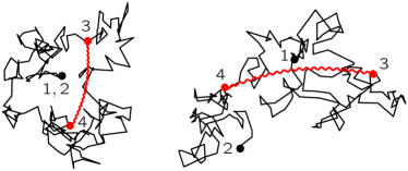
Figure 1: Random walks from $1\equiv(r_{1},-t/2)$ to $2\equiv(r_{2},+t/2)$, via $3\equiv(r_{3},t_{3})$ and $4\equiv(r_{4},t_{4})$: For given times $t,t_{3}$ and $t_{4}$, the distance between $r_{3}$ and $r_{4}$ is overestimated when the closed random walk (left) is substituted by an unrestricted random walk (right). This leads to increased decoherence and an underestimate of the weak-localization correction to the conductivity (see Fig. 2, dotted line).

At the corresponding point in their own work, CS make two further approximations when evaluating $F_{d}(t)$: firstly, they do not evaluate the vertex corrections explicitly, but instead mimic their effect by dropping (by hand) the contributions of frequency transfers $\bar{\omega}<1/t$ to the self-energy terms, i.e. they introduce a sharp infrared cutoff in the latter’s frequency integrals. Secondly, while averaging the correlators $\left\langle V_{3a}V_{4a^{\prime}}\right\rangle^{\textrm{cl}}$ of Eq. (27b) over random walks [i.e. averaging the Fourier exponents in Eq. (27b)], both CS and GZ employ the probability density ${\tilde{P}}^{\textrm{urw}}(r_{34},t_{34})$ for an unrestricted random walk to diffusively reach a volume element $d^{3}r$ removed by a distance $r_{34}=r_{3}-r_{4}$, in time $|t_{34}|$:

$$\left\langle e^{i{\bar{q}}(r(t_{3})-r(t_{4}))}\right\rangle_{\textrm{urw}} \equiv \int d^{3}r_{34}\,{\tilde{P}}^{\textrm{urw}}(r_{34},|t_{34}|)\,e^{i{\bar{q}}r_{34}}$$ (29)

$$\equiv {\bar{P}}^{\textrm{urw}}({\bar{q}},|t_{34}|)=e^{-D{\bar{q}}^{2}|t_{34}|}\,.\qquad\phantom{.}$$

Here and below, position integrals like $\int dr_{34}$ stand for $a^{3-d}\int d^{d}r$; the prefactor comes from the integral over the transverse directions, and it cancels the prefactor of ${\tilde{P}}^{\textrm{urw}}$ in Eq. (21a).

The two approximations discussed above are known to be adequate to correctly capture the functional dependence of the function $F(t)$ on time, temperature, dimensionless conductance, etc. In the following, however, we shall be more ambitious, and strive to evaluate the numerical prefactor of $F(t)$ with reasonable accuracy, too. To this end, we have to go beyond the two approximations of CS (dropping vertex terms and doing an unrestricted average), since both modify the numerical prefactor by a factor of order one: Firstly, we shall fully retain the vertex corrections; in effect, we thereby explicitly evaluate the actual shape of the effective infrared cutoff function, instead of inserting a sharp cutoff by hand. Secondly, we shall perform the random walk average more carefully than in Eq. (29), in that we consider only the actually relevant ensemble of closedMontambaux04 random walks of duration $t$, that are restricted to start and end at the same point in space: $r(-t/2)=r(t/2)=0$. Thus, we use

$$\left\langle e^{i{\bar{q}}(r(t_{3})-r(t_{4}))}\right\rangle_{\textrm{crw}} \equiv \int\!dr_{3}\,dr_{4}\,{\tilde{P}}^{\textrm{crw}}_{(0,t)}(3,4)\,e^{i{\bar{q}}r_{34}}$$ (30)

$$\equiv {\bar{P}}^{\textrm{crw}}_{(0,t)}({\bar{q}},|t_{34}|)\;.\qquad\phantom{.}$$

Here ${\tilde{P}}^{\textrm{crw}}_{(r_{12},t_{12})}(3,4)$ is the probability density for a closed random walk that starts at the space-time point $(r_{2},t_{2})$ and ends at $(r_{1},t_{1})$, to pass through two volume elements around the intermediate points $(r_{4},t_{4})$ and $(r_{3},t_{3})$. For $t_{2}<t_{4}<t_{3}<t_{1}$ we have

$${\tilde{P}}^{\textrm{crw}}_{(r_{12},t_{12})}(3,4)$$

$$=\frac{{\tilde{P}}^{\textrm{urw}}(r_{13},t_{13})\,{\tilde{P}}^{\textrm{urw}}(r_{34},t_{34})\,{\tilde{P}}^{\textrm{urw}}(r_{42},t_{42})}{{\tilde{P}}^{\textrm{urw}}(r_{12},t_{12})}\;.$$

The denominator ensures that the integral of ${\tilde{P}}^{\textrm{crw}}$ over $r_{4},r_{3}$ yields 1 [as can be seen using $\int dr_{3}\,{\tilde{P}}^{\textrm{urw}}(r_{13},t_{13})\,{\tilde{P}}^{\textrm{urw}}(r_{32},t_{32})={\tilde{P}}^{\textrm{urw}}(r_{12},t_{12})$]. We shall confirm below that ${\tilde{P}}^{\textrm{crw}}$ does not depend on $(r_{1},t_{1})$ and $(r_{2},t_{2})$ separately, but only on the differences $r_{12}$ and $t_{12}$, as anticipated on the left-hand side of Eq. (III.3).

The probability density ${\tilde{P}}^{\textrm{crw}}$ obviously does not depend on the magnetic field. Note, though, that Eq. (III.3) does not change if we multiply each factor ${\tilde{P}}^{\textrm{urw}}(r_{ij},t_{ij})$ by a dephasing factor $\exp(-t_{ij}/\tau_{H})$ to obtain a bare Cooperon ${\tilde{C}^{0}}(r_{ij},t_{ij})$, since these factors completely cancel out in Eq. (III.3). In the following, we shall thus use Eq. (III.3) with ${\tilde{P}}^{\textrm{urw}}$ replaced by ${\tilde{C}^{0}}$, since this will be convenient when comparing to perturbative expressions below, which are formulated in terms of ${\tilde{C}^{0}}$’s. Performing the integrals $\int dr_{3}dr_{4}$ of Eq. (30) by Fourier transformation and using

$$\bar{C}^{0}_{q}(t)=\theta(t)\,e^{-E_{q}t}\,,\qquad E_{q}\equiv Dq^{2}+1/{\tau_{H}}\,,$$ (32)

for the momentum Fourier transform of the bare Cooperon ${\tilde{C}^{0}}(r,t)$ of Eq. (21b), we readily find:

$${\bar{P}}^{\textrm{crw}}_{(r_{12},t_{12})}({\bar{q}},t_{34}) = {\int(dq)\,e^{iqr_{12}}\,\bar{C}^{0}_{q}(t_{13})\,\bar{C}^{0}_{q-{\bar{q}}}(t_{34})\,\bar{C}^{0}_{q}(t_{42})\over{\tilde{C}^{0}}(r_{12},t_{12})}$$ (33)

$$= e^{-D{\bar{q}}^{2}t_{34}\left(1-{t_{34}\over t_{12}}\right)+i{\bar{q}}r_{12}{t_{34}\over t_{12}}}\,.$$

In the limit $t_{12}\to\infty$ this reduces to ${\bar{P}}^{\textrm{urw}}({\bar{q}},t_{34})$, as expected, provided $t_{34}$ is kept fixed. Note, though, that the latter condition is not appropriate for the evaluation of the long-time limit of the Cooperon, for which both time differences, $t_{12}$ and $t_{34}$, become large.

III.4 General Form of the Decay Function $F(t)$

Let us now evaluate the decay function $F(t)=\langle S_{\textrm{eff}}\rangle_{\textrm{rw}}$, starting from the effective action of Eq. (27). Averaging the latter over time-reversed, random walks according to Eqs. (20) and (29) or (30), the result can be written as

$$F_{d}(t) = {1\over\hbar^{2}}\int_{-{t\over 2}}^{{t\over 2}}dt_{3}\int_{-{t\over 2}}^{{t\over 2}}dt_{4}\,\int(d\bar{q})\int(d\bar{\omega})\,e^{-i\bar{\omega}t_{34}}$$ (34)

$$\times\left\langle VV\right\rangle_{{\bar{q}}\bar{\omega}}^{\textrm{eff}}\,\delta{\bar{P}}({\bar{q}};\tau_{34},{\widetilde{\tau}}_{34})\;.$$

For classical noise, where $\langle V_{a}V_{a^{\prime}}\rangle_{{\bar{q}}{\bar{\omega}}}=\langle VV\rangle^{\textrm{cl}}_{{\bar{q}}{\bar{\omega}}}$, the “effective” environmental noise correlator appearing here likewise stands for the classical noise correlator, $\langle VV\rangle_{{\bar{q}}\bar{\omega}}^{\textrm{eff}}=\langle VV\rangle_{{\bar{q}}\bar{\omega}}^{\textrm{cl}}$. For the more general case that the $\langle V_{a}V_{a^{\prime}}\rangle_{{\bar{q}}{\bar{\omega}}}$ depend on $a,a^{\prime}$, as will be needed in our treatment of quantum noise below, the effective noise correlator is found to have the form

$$\left\langle VV\right\rangle_{{\bar{q}}\bar{\omega}}^{\textrm{eff}} = {\textstyle\frac{1}{2}}\left[\left\langle V_{F}V_{F}\right\rangle_{{\bar{q}}\bar{\omega}}+\left\langle V_{B}V_{B}\right\rangle_{{\bar{q}}\bar{\omega}}\right],\qquad\phantom{.}$$ (35a)

$$= {\textstyle\frac{1}{2}}\left[\left\langle V_{B}V_{F}\right\rangle_{{\bar{q}}\bar{\omega}}+\left\langle V_{F}V_{B}\right\rangle_{{\bar{q}}\bar{\omega}}\right],$$ (35b)

where, looking ahead, we used the fact that the first and second lines are equal for all the types of noise to be considered in this paper.

Eq. (34) also contains the object

$$\delta{\bar{P}}({\bar{q}};\tau_{34},{\widetilde{\tau}}_{34}) \equiv {\bar{P}}({\bar{q}},|t_{34}|)-{\bar{P}}({\bar{q}},|\widetilde{t}_{34}|)\qquad\phantom{.}$$ (36a)

$$= e^{-{\bar{q}}^{2}Dt\tau_{34}}-e^{-{\bar{q}}^{2}Dt{\widetilde{\tau}}_{34}}\;,$$ (36b)

which describes the diffusive dynamics of the time-reversed trajectories. The first term in Eq. (36) arises from self-energy terms [with $a=a^{\prime}$ in Eq. (27)], the second from vertex corrections [with $a\neq a^{\prime}$]. Here $\tau_{34}$ and ${\widetilde{\tau}}_{34}$ stand for

$$\tau_{34} = {|t_{34}|/t}\quad\textrm{or}\quad\tau_{34}=\left[1-{|t_{34}|/t}\right]{|t_{34}|/t}\;,\qquad\phantom{.}$$ (37a)

$${\widetilde{\tau}}_{34} = {|\widetilde{t}_{34}|/t}\quad\textrm{or}\quad{\widetilde{\tau}}_{34}=\left[1-{|\widetilde{t}_{34}|/t}\right]{|\widetilde{t}_{34}|/t}\;,\qquad\phantom{.}$$ (37b)

($\widetilde{t}_{34}=t_{3}+t_{4}$) depending on whether the average over paths is performed over unrestricted or closed random walks [using ${\bar{P}}^{\textrm{urw}}({\bar{q}},|t_{34}|)$ from Eq. (29) or ${\bar{P}}^{\textrm{crw}}_{(0,t)}({\bar{q}},t_{34})$ from Eq. (33)], respectively.

Since the time integrals in Eq. (34) are symmetric, only that part of $\left\langle VV\right\rangle_{{\bar{q}}\bar{\omega}}^{\textrm{eff}}$ that is symmetric under ${\bar{\omega}}\to-{\bar{\omega}}$ contributes to $F_{d}(t)$; moreover, if this symmetric part is real, so is $F_{d}(t)$.

The fact that the decay function is linear in interaction propagators has an important implication: when expanding both sides of Eq. (LABEL:completeAvgRRW) in powers of the interaction, the term linear in $F_{d}(t)$ on the right-hand side of Eq. (LABEL:completeAvgRRW) must equal ${\tilde{C}}^{1}(0,t)$, the first-order contribution to the full Cooperon ${\tilde{C}}(0,t)$, implying $-F_{d}^{\textrm{crw}}(t)={\tilde{C}}^{1}(0,t)/{\tilde{C}^{0}}(0,t)$ [cf. Eq. (4a)]. We added the superscript “crw”, because this relation turns out to hold only if the average over paths for $F_{d}(t)$ is over closed random walks. The expression (LABEL:eq:CooperondecaywithF) for ${\tilde{C}}(0,t)$ thus amounts to a simple reexponentiation of the first order interaction correction,

$${\tilde{C}}(0,t)\simeq{\tilde{C}^{0}}(0,t)\exp\left[\frac{{\tilde{C}}^{1}(0,t)}{{\tilde{C}^{0}}(0,t)}\right]\,,$$ (38a)

evaluated in the position-time representation (at $$r=0 {\bar{P}}^{\textrm{urw}} {\bar{P}}^{\textrm{crw}} -F_{d}^{\textrm{urw}}(t)=\int dr\,{\tilde{C}}^{1}_{\gamma_{H}=0}(r,t)=\bar{C}_{q=\gamma_{H}=0}^{1}(t)$$). In contrast, if (following hitherto standard practiceCS ; GZ2 ) the average over paths is performed over unrestricted random walks instead, i.e. if is used instead of in (34), one finds [cf. Eq. (4b)]. In this case Eq. (LABEL:eq:CooperondecaywithF) yields

$${\tilde{C}}(0,t)\simeq{\tilde{C}^{0}}(0,t)\exp\left[\bar{C}_{\gamma_{H}=q=0}^{1}(t)\right]\,,$$ (38b)

implying that here the first order correction in the momentum-time representation is reexponentiated; consequently, the left- and right-hand sides of Eq. (38b) are not consistent when expanded to first order in the interaction. Hence, Eq. (38a) can be expected to be more accurate than (38b), as will be confirmed below.

To make further progress with the evaluation of $F(t)$, we now exploit the fact that for all types of noise to be considered in this paper, the effective noise correlator factorizes into a frequency-dependent spectrum ${\mathcal{W}}_{\textrm{eff}}({\bar{\omega}})$, symmetric in frequency, and a ${\bar{q}}$-dependent denominator:

$${\textstyle{1\over\hbar}}\left\langle VV\right\rangle^{\textrm{eff}}_{{\bar{q}}\bar{\omega}} = {{\mathcal{W}}_{\textrm{eff}}(\bar{\omega})\over\nu D{\bar{q}}^{2}}\;.$$ (39)

This fact allows us to proceed quite far with the evaluation of Eq. (34) for $F_{d}(t)$ without specifying the actual form of ${\mathcal{W}}_{\textrm{eff}}(\bar{\omega})$ (which will be done in later sections): after changing integration variables to the sum and difference times $\widetilde{t}_{34}$ and $t_{34}$, Eq. (34) can be written as

$$F_{d}(t) = 2\!\int_{0}^{t}\!\!dt_{34}\,W_{\textrm{eff}}(t_{34})\!\int_{0}^{t-t_{34}}\!\!d\widetilde{t}_{34}\,\delta{\tilde{P}}_{d}(\tau_{34},{\widetilde{\tau}}_{34})\;,\qquad\phantom{.}$$ (40)

where the kernel

$$W_{\textrm{eff}}(t_{34})=\int(d\bar{\omega})\,e^{-i\bar{\omega}t_{34}}{\mathcal{W}}_{\textrm{eff}}(\bar{\omega})\;$$ (41)

contains all information about the frequency-dependence of the noise correlator describes the range in time of the effective interaction, whereas the dimensionless quantity

$$\delta{\tilde{P}}_{d}(\tau_{34},{\widetilde{\tau}}_{34}) = \int(d\bar{q})\,{e^{-{\bar{q}}^{2}Dt\tau_{34}}-e^{-{\bar{q}}^{2}Dt{\widetilde{\tau}}_{34}}\over{\hbar}\nu D{\bar{q}}^{2}}\qquad\phantom{.}$$ (42)

is the same for all types of noise studied below, but depends on the dimensionality of the sample. Note that the integrand in Eq. (42) is well-behaved for small ${\bar{q}}^{2}$ despite of the $1/{\bar{q}}^{2}$ factor, because the self-energy and vertex contributions to $\delta{\bar{P}}({\bar{q}};\tau_{34},{\widetilde{\tau}}_{34})$ [Eq. (36)] cancel each other for momentum transfers smaller than $D{\bar{q}}^{2}\lesssim 1/t$, thus regularizing the divergence. This is precisely as expected for density fluctuations with dispersion $\bar{\omega}\simeq D{\bar{q}}^{2}$: on time scales of order $t$, fluctuations with frequencies below $\bar{\omega}\lesssim 1/t$ appear to be essentially static, and hence do not contribute to decoherence.

The $\int(d{\bar{q}})$ and $\int d\widetilde{t}_{34}$ integrals in Eqs. (42) and (40) can be performed explicitly (see App. A), with a result for $F_{d}(t)$ of the form

$$F_{d}(t)={t\over g_{d}(L_{t})}\int_{0}^{t}dt_{34}\,W_{\textrm{eff}}(t_{34})\,{{\cal P}}_{d}(t_{34}/t)\;,$$ (43)

where $L_{t}=\sqrt{Dt}$. Explicit expressions for the functions ${{\cal P}}_{d}(z)$, which differ for closed or unrestricted random walks, are given in App. A. However, it will turn out below that we really only need the leading terms in an expansion of $P_{d}(z)$ for small values of its arguments, because the decoherence rate is extracted from the long-time behavior of $F_{d}(t)$. The leading and subleading terms of ${{\cal P}}_{d}^{\textrm{crw}}$ for closed or ${{\cal P}}_{d}^{\textrm{urw}}$ for unrestricted random walks (upper or lower entries, respectively) are given by:

$${{\cal P}}_{1}^{\{\stackrel{{\scriptstyle\textrm{crw}}}{{\scriptscriptstyle\textrm{urw}}}\}}(z) = \left\{\begin{array}[]{l}\sqrt{\pi}/2\\ 8/(3\sqrt{\pi})\end{array}\right\}-{4\sqrt{z/\pi}}+{\cal O}(z)\;,\qquad\phantom{.}$$ (44c)

$${{\cal P}}_{2}^{\{\stackrel{{\scriptstyle\textrm{crw}}}{{\scriptscriptstyle\textrm{urw}}}\}}(z) = -{1\over\pi}\left[\ln z+\left\{\begin{array}[]{l}2+{\cal O}(z)\\ 1+{\cal O}(z\ln z)\end{array}\right\}\right]\;,$$ (44f)

$${{\cal P}}_{3}^{\{\stackrel{{\scriptstyle\textrm{crw}}}{{\scriptscriptstyle\textrm{urw}}}\}}(z) = {1\over\pi^{3/2}}\left[{1\over\sqrt{z}}-\left\{\begin{array}[]{l}\pi\\ 2\end{array}\right\}\right]+{\cal O}(z^{1/2})\;.$$ (44i)

Thus, the difference between averaging over closed or unrestricted random walks turns out to matter for the leading terms of only ${{\cal P}}_{1}$ (but not of ${{\cal P}}_{2,3}$), implying, as we shall see below, that it matters for the leading long-time behavior of only $F_{1}(t)$ [but not of $F_{2,3}(t)$].

Eq. (43) is a central result on which the following sections rely. To find the decay function $F_{d}(t)$ (and a corresponding decoherence time), all that remains to be done is to determine the spectrum ${\mathcal{W}}_{\textrm{eff}}(\bar{\omega})$ (which depends on the type of noise studied, and on whether the Pauli principle is taken care of), calculate its Fourier transform to obtain the kernel $W_{\textrm{eff}}(t_{34})$ of Eq. (41), and perform the integral $\int dt_{34}$ in Eq. (43).

We close this section with a comment on the relation of the above approach to diagrammatic methods, e.g. the calculation of the Cooperon ${\tilde{C}}^{1}(0,t)$ to first order in the interaction (from which $F_{d}(t)$ can be extracted). The key to our derivation of Eq. (43) was to essentially work in the time domain, postponing any time integrals until after all momentum and frequency integrals had been performed, as exemplified by our definitions of ${\tilde{P}}^{\textrm{crw}}$ [Eq. (33), involving $\int(dq)$], $\delta{\tilde{P}}_{d}$ [Eq. (42), involving $\int(d{\bar{q}})$] and $W(t_{34})$ [Eq. (41), involving $\int(d\bar{\omega})$]. In contrast, in diagrammatic calculations, the $\int dt_{3}dt_{4}$ integrals are performed first (namely when deriving the Feynman rules for the frequency-momentum), before any momentum or frequency intetrals. However, for the present problem the resulting momentum integrals then take intractably complicated forms (see App. B).

Nevertheless, for the case of unrestricted random walks, the leading asymptotic behavior of $F_{d,\textrm{urw}}(t)$ can be obtained rather simply by judiciously neglecting some terms that are subleading in the limit of large times. As shown in App. B, this leads to the following expression,

$$F_{d,\textrm{urw}}(t) \simeq p_{d}\,t\int_{0}^{\infty}\!\!{d\bar{\omega}}\,{{\mathcal{W}}_{\textrm{eff}}(\bar{\omega})\over\bar{\omega}^{2-d/2}}\left[1-{\sin(\bar{\omega}t)\over\bar{\omega}t}\right],\qquad\phantom{.}$$ (45)

with $p_{1}=\sqrt{2\gamma_{1}}/\pi$, $p_{2}=1/(g_{2}2\pi)$, $p_{3}=1/(\sqrt{2\gamma_{3}}\,\pi^{2})$ [for $\gamma_{1},g_{2},\gamma_{3}$, see Eq. (11)]. This formula for $F_{d,\textrm{urw}}(t)$ is less accurate than Eq. (43), but perhaps physically more transparent, since formulated in the frequency domain: The factor $[1-\sin(\bar{\omega}t)/\bar{\omega}t]$ acts as infrared cutoff, suppressing frequencies $\bar{\omega}\lesssim 1/t$. Due to the factor $\bar{\omega}^{d/2-2}$, the integral gets its dominant contribution from small frequencies of order $1/t$ for $d=1$, gets logarithmic contributions from both small and large frequencies for $d=2$, and is dominated by large frequencies for $d=3$. In particular, for $d=2,3$ an ultraviolet cutoff is needed at large frequencies to render the integral well-defined. As we shall see below, such a cutoff will be provided by ${\mathcal{W}}_{\textrm{eff}}(\bar{\omega})$.

III.5 Comparison with exact classical 1-D result

To gauge quantitatively the difference between averaging over closed or unrestricted random walks, we shall now use the above results to calculate the magnetoconductivity for a quasi 1-dimensional conductor and classical white Nyquist noise. For this particular case, the average $\langle e^{-S_{\textrm{eff}}{/\hbar}}\rangle_{\textrm{rrw}}$ was calculated exactly by AAK,AAK so that the resulting expression for the magnetoconductivity,factorof2

$$\delta\sigma_{{\textrm{exact}}}^{\rm WL}=\frac{e^{2}\sqrt{D\tau^{\scriptscriptstyle{\rm AAK}}_{\varphi}}}{\pi{\hbar}}\frac{1}{[\ln{\rm Ai}(\frac{\tau_{\varphi}^{\rm AAK}}{\tau_{H}})]^{\prime}}\,,$$ (46)

can be used as benchmark for other approximations. In Eq. (46), Ai is the Airy function, and $\tau_{\varphi}^{\scriptscriptstyle{\rm AAK}}$ is the decoherence time of Eq. (6).

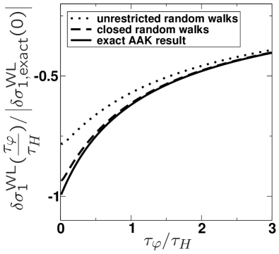
Figure 2: The magnetoconductivity for a quasi 1-dimensional wire experiencing decoherence by classical white Nyquist noise, as function of $\tau_{\varphi,1}^{\scriptscriptstyle{\rm AAK}}/{\tau_{H}}$, comparing AAK’s exact Airy function result (46), solid line, against two approximations: the commonly employed average over unrestricted random walks in the path-integral exponent, [Eq. (38b)], and the improved version obtained by averaging over closed random walks [Eq. (38a)], resulting in Eq. (50), with $c_{1}^{\textrm{urw}}$ or $c_{1}^{\textrm{crw}}$, respectively. For $\tau_{\varphi}/\tau_{H}\rightarrow 0$, the result for unrestricted (closed) random walks equals $0.808$ ($0.964$) of the exact value. For $\tau_{\varphi,1}^{\scriptscriptstyle{\rm AAK}}/\tau_{H}\gg 1$, all three curves become indistinguishable.

For the particular case of classical white Nyquist noise, the noise correlator is given by $T/\nu D{\bar{q}}^{2}$, so that the effective noise correlator of Eq. (34) takes the form:

$${\textstyle{1\over\hbar}}\left\langle VV\right\rangle_{{\bar{q}}\bar{\omega}}^{\textrm{eff}}\mapsto{\textstyle{1\over\hbar}}\left\langle VV\right\rangle_{{\bar{q}}\bar{\omega}}^{\textrm{cl}}=\frac{T}{\nu D{\bar{q}}^{2}}\;.$$ (47)

Thus, the weighting function in Eq. (39) is frequency-independent for classical white Nyquist noise, ${\mathcal{W}}_{\textrm{cl}}({\bar{\omega}})=T$, so that the corresponding Kernel is an infinitely sharp delta function, $W_{\textrm{cl}}(t_{34})=T\delta(t_{34})$. The $\int dt_{34}$ integral in Eq. (43) for $F_{1}^{\textrm{cl}}(t)$ is thus easily performed, yielding

$$F^{\textrm{cl}}_{1}(t) = c_{1}{tT\over g_{1}(L_{t})}=(t/\tau_{\varphi,1})^{3/2}\;,\quad\begin{array}[]{c}c_{1}^{\textrm{crw}}={\sqrt{\pi}\over 4}\;,\rule[-8.53581pt]{0.0pt}{0.0pt}\\ c_{1}^{\textrm{urw}}={4\over 3\sqrt{\pi}},\end{array}\qquad\phantom{.}$$ (50)

where $\tau_{\varphi,1}=(c_{1}\sqrt{\gamma_{1}}T)^{-2/3}$. Depending on whether we average over closed or unrestricted random walks, two different values for the prefactor $c_{1}$ are obtained. The decoherence time was obtained by solving $F^{\textrm{cl}}_{1}(\tau_{\varphi,1})=1$ for $\tau_{\varphi,1}$, which reproduces Eq. (6), with an extrathresholdconstant $c_{1}$ in front of $T$.

The fact that $\tau^{\textrm{crw}}_{\varphi,1}$ is somewhat larger than $\tau^{\textrm{urw}}_{\varphi,1}$ (the relative factor is $(16/3\pi)^{2/3}=1.423$) can intuitively be understood from Fig. 1: For a given time difference $t_{34}$, the distance $r_{34}$ between the points $r_{3}$ and $r_{4}$ is overestimated on average when closed random walks are replaced by unrestricted random walks. Thus the latter give somewhat too much weight to the effect of long wavelength or small momentum transfers, which dominate the integral in Eqs. (42). They hence somewhat overestimate the decoherence rate, and consequently underestimate the decoherence time and magnitude of the weak localization correction to the conductivity [cf. Fig. 2].

The weak localization contribution to the magnetoconductivity $\delta\sigma_{1}^{\rm WL}$ of a quasi 1-dimensional wire can now be obtained by inserting $F_{1}^{\textrm{cl}}(t)$ of Eqs. (50) into Eq. (22). Fig. 2 compares the results so obtained using $c_{1}^{\textrm{urw}}$ (dotted line) and $c_{1}^{\textrm{crw}}$ (dashed line) to AAK’s Airy function result [Eq. (46), solid line]. Firstly and most importantly, all three approaches agree fully in their predition for ${\tau_{\varphi}}$, which acts as the scale on which the magnetoconductivity is suppressed as a function of increasing magnetic field (i.e. increasing $1/{\tau_{H}}$). However, the methods differ somewhat in their predictions for the magnetoconductivity $\delta\sigma^{\rm WL}_{1}$ at $B=0$, which gives the overall magnitude of the weak localization effect: Averaging over unrestricted random walks (dotted line) yields only qualitative agreement with the exact Airy-function result, deviating from it by about 20% at $B=0$. In contrast, averaging over closed random walks (dashed line) gives excellent quantitative agreement with the exact result, yielding practically identical results for large and intermediate field strengths, with a maximal deviation of less than 4% in the limit of vanishing magnetic field. It is quite remarkable that such good agreement with an exact result can be obtained by means as elementary as the above.

IV Cooperon decay for quantum noise without Pauli principle

Inspired by the simplicity and elegance of the above treatment of classical noise fields, we shall explore in this section to what extent a quantum bath can be similarly dealt with in a single-particle path integral picture: is it possible to identify suitably chosen “effective classical noise” correlators, such that the decay function $F(t)$ is again of the form (40), with $\langle VV\rangle_{{\bar{q}}\bar{\omega}}^{\textrm{cl}}$ replaced by some suitably chosen effective noise correlator $\langle VV\rangle_{{\bar{q}}\bar{\omega}}^{\textrm{eff}}$? The advantage of such a formulation would evidently be (i) that the results are sure to be free of infrared problems, and (ii) that the trajectory averages could be performed with the same ease as above.

Of course, we know from the outset that a strategy based on mimicking quantum by classical noise fields can never be exact or complete, because the correlator $\angle\hat{V}\hat{V}\rangle_{\bar{q}\bar{\omega}}$ of a quantum noise field differs from that of a classical noise field in an elementary but fundamental way: In contrast to $\langle VV\rangle_{\bar{q}\bar{\omega}}^{\textrm{cl}}$ , which is symmetric in frequency, $\langle\hat{V}\hat{V}\rangle_{\bar{q}\bar{\omega}}$ is asymmetric in frequency, reflecting the asymmetry between energy absorption from ($\bar{\omega}<0$) and emission into ($\bar{\omega}>0$) the bath, $\bar{\omega}$ being the change in bath energy. In particular, the asymmetry manifests itself in the possibility of spontaneous emission events which are possible even at $T=0$, and hence strongly affect the low-temperature behavior. Nevertheless, we shall see that when the effective action is evaluated along time-reversed paths as needed to describe the decay of the Cooperon, it is again governed by a noise correlator symmetric in frequency, so that this decay can be described by a suitably-chosen ”effective” classical noise field.

IV.1 Definition of quantum noise correlators

We begin by recalling that for a free bosonic quantum field $\hat{V}_{j}\equiv\hat{V}(r_{j},t_{j})$, the two correlation functions

$$-i{\hbar}\tilde{\mathcal{L}}_{ij}^{>}=\bigl{\langle}\hat{V}_{i}\hat{V}_{j}\bigr{\rangle}\;,\qquad-i{\hbar}\tilde{\mathcal{L}}_{ij}^{<}=\bigl{\langle}\hat{V}_{j}\hat{V}_{i}\bigr{\rangle}\;,$$ (51)

are not equal (as would be the case for a classical field), but are related, after Fourier transforming, by the detailed-balance relation $\bar{\mathcal{L}}_{{\bar{q}}}^{<}(\bar{\omega})=e^{-\beta\bar{\omega}}\bar{\mathcal{L}}_{{\bar{q}}}^{>}(\bar{\omega})$. This implies that the symmetrized and anti-symmetric correlators, or, equivalently, the Keldysh, retarded and advanced correlators

$$-i{\hbar}\tilde{\mathcal{L}}_{ij}^{K} = \bigl{\langle}\{\hat{V}_{i},\hat{V}_{j}\}\bigr{\rangle}\;,$$ (52a)

$$-i{\hbar}\tilde{\mathcal{L}}_{ij}^{R/A} = \pm\theta(\pm t_{ij})\bigl{\langle}[\hat{V}_{i},\hat{V}_{j}]\bigr{\rangle}\;,$$ (52b)

are related by the fluctuation-dissipation theorem,

$$-{\textstyle\frac{1}{2}}i\bar{\cal L}^{K}_{{\bar{q}}}(\bar{\omega}) = \textrm{Im}\bar{\cal L}^{R}_{{\bar{q}}}(\bar{\omega})\,\coth\Bigl{[}\frac{\bar{\omega}}{2T}\Bigr{]}\;,$$ (53a)

$$= \textrm{Im}\bar{\cal L}^{R}_{{\bar{q}}}(|\bar{\omega}|)\,\bigl{[}2n(|\bar{\omega}|)+1\bigr{]}\;,\qquad\phantom{.}$$ (53b)

where $\textrm{Im}\bar{\cal L}^{R}_{{\bar{q}}}(\bar{\omega})={1\over 2{\hbar}}\bigl{\langle}[\hat{V},\hat{V}]\bigr{\rangle}_{{\bar{q}}\bar{\omega}}$ is an odd function of $\bar{\omega}$. For example, the noise generated by the standard screened Coulomb interaction, namely quantum Nyquist noise (which we shall focus on for the remainder of this paper), can be described by taking

$$\textrm{Im}\bar{\mathcal{L}}_{{\bar{q}}}^{R}(\bar{\omega}) = {{\bar{\omega}}\over 2\nu D{\bar{\bm{q}}}^{2}}$$ (54)

[see, e.g., Refs. AAG, or vonDelft04, ]. Using the above relations, the quantum noise correlator can be written as

$${\textstyle{1\over\hbar}}\bigl{\langle}\hat{V}\hat{V}\bigr{\rangle}_{{\bar{q}}\bar{\omega}} = \textrm{Im}\bar{\cal L}^{R}_{{\bar{q}}}(|\bar{\omega}|)\,\bigl{[}2n(|\bar{\omega}|)+2\theta(\bar{\omega})\bigr{]}\;.$$ (55)

In Eq. (55), the contribution of $n(|\bar{\omega}|)$ dominates at frequency transfers smaller than the temperature, for which the number of activated quanta is large ($n\gg 1$). The additional step function $\theta(\bar{\omega})$, responsible for the asymmetry of $\bigl{\langle}\hat{V}\hat{V}\bigr{\rangle}_{{\bar{q}}\bar{\omega}}$, contributes even if the bath is at zero temperature ($n=0$), and hence is sometimes said to reflect zero-point fluctuations of the bath. It describes the possibility of spontaneous emission of energy by the electron into the bath, enabling excited electrons to relax to states of lower energy. Of course, in a many-body situation, the rates for such relaxation processes will also contain Fermi functions that Pauli-block them if no empty final states are available. However, we shall defer a detailed discussion of Pauli blocking to Section V and completely ignore it in the present section, which thus applies only to situations for which Pauli restrictions are irrelevant. The latter would include a purely single-particle problem, or, for a many-body degenerate Fermi gas, an electron that is very highly excited above the Fermi surface, with plenty of empty states below to decay into.

IV.2 Averaging over quantum noise

It is known FeynmanHibbs64 that the effects of a quantum noise field $\hat{V}(r,t)$ on a quantum particle can be described in terms of classical (c-number) fields by proceeding as follows: one considers a path-integral with a Keldysh forward-backward contour, and includes the noise via phase factors $e^{-i\int dx_{j}dt_{j}V_{jF}{/\hbar}}$ (as part of $e^{iS_{F}{/\hbar}}$) and $e^{i\int dx_{j}dt_{j}V_{jB}{/\hbar}}$ (as part of $e^{-iS_{B}{/\hbar}}$) that contain two different fields, $V_{jF}=V_{F}(r_{j},t_{j})$ and $V_{jB}=V_{B}(r_{j},t_{j})$, on the forward- and backward-contour, respectively. [In the case of classical noise the Keldysh fields are equal, $V_{F}=V_{B}=V$.] The classical field correlators are related to the quantum noise field correlators $\bigl{\langle}\hat{V}_{i}\hat{V}_{j}\bigr{\rangle}$ of Eqs. (51) by time-ordering along the Keldysh contour:

$$\bigl{\langle}V_{iF}V_{jF}\bigr{\rangle} \equiv \bigl{\langle}\hat{T}\hat{V}_{i}\hat{V}_{j}\bigr{\rangle}=-{\textstyle{{\hbar\over{2}}}}i(\tilde{\cal L}^{K}+\tilde{\cal L}^{R}+\tilde{\cal L}^{A})_{ij}\;,\qquad\phantom{.}$$ (56a)

$$\bigl{\langle}V_{iB}V_{jB}\bigr{\rangle} \equiv \bigl{\langle}\tilde{\hat{T}}\hat{V}_{i}\hat{V}_{j}\bigr{\rangle}=-{\textstyle{{\hbar\over{2}}}}i(\tilde{\cal L}^{K}-\tilde{\cal L}^{R}-\tilde{\cal L}^{A})_{ij}\;,\qquad\phantom{.}$$ (56b)

$$\bigl{\langle}V_{iB}V_{jF}\bigr{\rangle} \equiv \bigl{\langle}\hat{V}_{i}\hat{V}_{j}\bigr{\rangle}\phantom{\hat{T}}=-{\textstyle{{\hbar\over{2}}}}i(\tilde{\cal L}^{K}+\tilde{\cal L}^{R}-\tilde{\cal L}^{A})_{ij}\;,\qquad\phantom{.}$$ (56c)

$$\bigl{\langle}V_{iF}V_{jB}\bigr{\rangle} \equiv \bigl{\langle}\hat{V}_{j}\hat{V}_{i}\bigr{\rangle}\phantom{\hat{T}}=-{\textstyle{{\hbar\over{2}}}}i(\tilde{\cal L}^{K}-\tilde{\cal L}^{R}+\tilde{\cal L}^{A})_{ij}\;.\qquad\phantom{.}$$ (56d)

The first set of relations in Eqs. (56) follows from comparing the expansions generated when expanding the factors $e^{-i\int dx_{j}dt_{j}V_{jF}{/\hbar}}$ occuring in a time-ordered path integral for the forward path, and $e^{i\int dx_{j}dt_{j}V_{jB}{/\hbar}}$ occuring in a backward path, with the corresponding expansions of the quantum time evolution operators $\hat{U}_{F}=\hat{T}e^{-i\int dx_{j}dt_{j}\hat{V}_{j}{/\hbar}}$ and $\hat{U}_{B}^{\dagger}=\tilde{\hat{T}}e^{i\int dx_{j}dt_{j}\hat{V}_{j}{/\hbar}}$ occuring in Keldysh perturbation theory, respectively. The second set of relations in Eqs. (56) are simply standard identities, following from the definitions (52) of $\tilde{\mathcal{L}}_{ij}^{K,R,A}$.

The effective action for a single-particle subject to such quantum noise (sqn), to be denoted by $S_{\textrm{eff}}^{\textrm{sqn}}$, is obtained as for Eq. (26): we now have to perform a Gaussian average over $V_{F},V_{B}$, again with the action $i(S_{F}-S_{B})$ of Eq. (25) in the exponent, but now with $V_{ja}\equiv V_{a}(r^{a}(t_{j}),t_{j})$, i.e. both the paths $r^{a}(t)$ and the fields $V_{a}$ differ on the forward and backward contours. The result for $S^{\textrm{sqn}}_{\textrm{eff}}$ again has the form of Eqs. (27), but now $\bigl{\langle}V_{a}V_{a^{\prime}}\bigr{\rangle}_{{\bar{q}}{\bar{\omega}}}$ stands for the Fourier transform of the quantum correlators of Eqs. (56). In fact, $e^{-S^{\textrm{sqn}}_{\textrm{eff}}{/\hbar}}$ is nothing but the Feynman-Vernon influence functional for a single particle interacting with a quantum bath. Note that in contrast to the effective action for classical noise, $S^{\textrm{sqn}}_{\textrm{eff}}$ is in general complex, since the correlators $\bigl{\langle}V_{ia}V_{ja^{\prime}}\bigr{\rangle}$ are all complex (because $-i\tilde{\cal L}^{K}_{ij}$, $\tilde{\cal L}^{R}_{ij}$ and $\tilde{\cal L}^{A}_{ij}$ are by construction purely real).

IV.3 Quantum noise spectrum without Pauli principle

To describe the effect of quantum noise on the Cooperon, the influence functional $e^{-S^{\textrm{sqn}}_{\textrm{eff}}{/\hbar}}$ has to be averaged over all time-reversed pairs of closed random walks. This can be done in the same way as as in Section III.3. The result for $F_{d}^{\textrm{sqn}}(t)\equiv{1\over\hbar}\langle S^{\textrm{sqn}}_{\textrm{eff}}\rangle_{\textrm{rw}}$ has the same form as Eq. (34),

$$F_{d}^{\textrm{sqn}}(t) = {1\over\hbar^{2}}\int_{-{t\over 2}}^{{t\over 2}}dt_{3}\int_{-{t\over 2}}^{{t\over 2}}dt_{4}\,\int(d\bar{q})\int(d\bar{\omega})\,e^{-i\bar{\omega}t_{34}}$$ (57)

$$\times\left\langle VV\right\rangle_{{\bar{q}}\bar{\omega}}^{\textrm{sqn}}\,\delta{\bar{P}}({\bar{q}};\tau_{34},{\widetilde{\tau}}_{34})\;,$$

where the effective noise correlator in Eq. (34) now takes the form [obtained from Eqs. (35) and Eqs. (56)]:

$$\bigl{\langle}VV\bigr{\rangle}_{{\bar{q}}\bar{\omega}}^{\textrm{eff}}\mapsto\bigl{\langle}VV\bigr{\rangle}_{{\bar{q}}\bar{\omega}}^{\textrm{sqn}}=-{\textstyle{\hbar\over{2}}}i\bar{\cal L}^{K}_{{\bar{q}}\bar{\omega}}\,=\,{\textstyle\frac{1}{2}}\bigl{\langle}\{\hat{V},\hat{V}\}\bigr{\rangle}_{{\bar{q}}\bar{\omega}}.\quad\phantom{.}$$ (58a)

For the case of quantum Nyquist noise [Eq. (54)], $${1\over\hbar}\langle VV\rangle_{{\bar{q}}\bar{\omega}}^{\textrm{sqn}} {{\mathcal{W}}_{\textrm{sqn}}/\nu D{\bar{q}}^{2}}$$ can be written in the factorized form of Eqs. (39), the corresponding spectrum being

$${\mathcal{W}}_{\textrm{sqn}}({\bar{\omega}})={\textstyle\frac{1}{2}}|{\bar{\omega}}|\bigl{[}2n(|{\bar{\omega}}|)+1\bigr{]}\;.$$ (58b)

Just as for classical noise, this effective noise spectrum is symmetric in ${\bar{\omega}}$ and ${\bar{q}}$ and real [as follows from Eq. (53b)], which implies that $F^{\textrm{sqn}}_{d}(t)$ is purely real. In other words, the imaginary part of the effective action $S^{\textrm{sqn}}_{\textrm{eff}}$ vanishes upon averaging over time-reversed paths; the reason is that (the Fourier transforms of) the purely imaginary $\mp{\textstyle\frac{1}{2}}i(\bar{\cal L}^{R}+\bar{\cal L}^{A})$ contributions from Eqs. (56a) and (56b) cancel each other when inserted into Eq. (35), as do the contributions $\mp{\textstyle\frac{1}{2}}i(\bar{\cal L}^{R}-\bar{\cal L}^{A})$ from Eqs. (56c) and (56d).

The fact that $\langle S_{\textrm{eff}}^{\textrm{sqn}}\rangle_{\textrm{crw}}$ is purely real along time-reversed paths has the following useful implication: for the particular purpose of calculating the Cooperon decay, it is possible to mimick the effect of a quantum-mechanical environment by a purely classical noise field, if we so wish, provided its noise correlator is postulated to be given precisely by $\langle VV\rangle_{{\bar{q}}\bar{\omega}}^{\textrm{sqn}}$ of Eq. (58), i.e. the symmetrized version of the asymmetric quantum noise correlator (55). This can be verified by rewriting the effective action in terms of even and odd combinations of $V_{F/B}$, namely

$$V_{+j}={\textstyle\frac{1}{2}}(V_{Fj}+V_{Bj})\;,\qquad\ V_{-j}=V_{Fj}-V_{Bj}\;.$$ (59)

It is then readily found that the decay of the Cooperon is governed only by the even field $V_{j+}$; indeed, since their correlators are given by

$${\displaystyle\left(\begin{array}[]{cc}\bigl{\langle}V_{+i}V_{+j}\bigr{\rangle}&\bigl{\langle}V_{+i}V_{-j}\bigr{\rangle}\rule[-8.53581pt]{0.0pt}{0.0pt}\\ \bigl{\langle}V_{-i}V_{+j}\bigr{\rangle}&\bigl{\langle}V_{-i}V_{-j}\bigr{\rangle}\end{array}\right)=-i{\hbar}\left(\begin{array}[]{cc}{\textstyle\frac{1}{2}}\tilde{\mathcal{L}}_{ij}^{K}&\tilde{\mathcal{L}}_{ij}^{R}\rule[-8.53581pt]{0.0pt}{0.0pt}\\ \phantom{{\textstyle\frac{1}{2}}}\tilde{\mathcal{L}}_{ij}^{A}&0\end{array}\right)},\quad\phantom{.}$$ (64)

we see that the symmetrized noise correlator $\langle VV\rangle^{\textrm{sqn}}_{{\bar{q}}{\bar{\omega}}}$ governing the Cooperon decay function $F^{\textrm{sqn}}_{d}(t)$ is equal to the correlator $\langle V_{+}V_{+}\rangle_{{\bar{q}}{\bar{\omega}}}$ of the even field $V_{+j}$, whereas the correlators $\langle V_{\pm}V_{\mp}\rangle_{{\bar{q}}{\bar{\omega}}}$ involving the odd field play no role in determining $F^{\textrm{sqn}}_{d}(t)$.

IV.4 The effect of spontaneous emission

It is instructive to analyse the differences between the classical spectrum ${\mathcal{W}}_{\textrm{cl}}({\bar{\omega}})=T$ and the quantum case ${\mathcal{W}}_{\textrm{sqn}}({\bar{\omega}})$ of Eq. (58b). Since both are symmetric in ${\bar{\omega}}$, the main qualitative difference between them is the presence in the quantum case of spontaneous emission, leading to an extra contribution that does not vanish at zero temperature. Although spontaneous emission only enhances the scattering rate for transitions downward in energy, the preceding analysis shows that the asymmetric quantum noise spectrum may just as well be replaced by its symmetrized version. Physically, this is possible because both the upward and downward transitions are equally effective in contributing to dephasing (if they are allowed), and thus it is only their sum that matters for the dephasing rate. Schematically, we have

$$\Gamma_{\varphi} = {1\over 2}(\Gamma_{\uparrow}+\Gamma_{\downarrow})$$ (65)

$$\propto {1\over 2}(n+(n+1))$$

$$= {1\over 2}([n+{1\over 2}]+[n+{1\over 2}]),$$

where $n=n(|\bar{\omega}|)$ is the Bose occupation number for the frequency transfer $\bar{\omega}$ under consideration.

This procedure is possible for a single, excited electron without Fermi sea, or, in a many-body situation, for an electron so highly excited above the Fermi sea that Pauli restrictions on the available final states are negligible. In such a case, spontaneous emission processes evidently persist down to zero temperature and will thus cause the decoherence rate to remain finite even at $T=0$ [see also Ref. FMSR, ]. Indeed, this can be seen explicitly from Eq. (45) for $F_{d,\textrm{urw}}^{\textrm{sqn}}(t)$: replacing ${\mathcal{W}}_{\textrm{eff}}(\bar{\omega})$ therein by the single-particle quantum noise spectrum at zero temperature, ${\mathcal{W}}^{(T=0)}_{\textrm{sqn}}({\bar{\omega}})={\textstyle\frac{1}{2}}|\bar{\omega}|$, and introducing an upper cutoff $\int_{0}^{\bar{\omega}_{\rm u}}d\bar{\omega}$ to regularize the ultraviolet divergence that then arises, one readily finds that $F_{d,\textrm{urw}}^{\textrm{sqn}}(t)={1\over d}p_{d}\,\bar{\omega}_{\rm u}^{d/2}t$, implying a finite decoherence rate at zero temperature:

$$\gamma_{\varphi,d}^{\textrm{sqn}(T=0)}={\textstyle{1\over d}}p_{d}\,\bar{\omega}_{\rm u}^{d/2}\;.$$ (66)

V Decoherence and the Pauli principle

The scenario discussed at the end of the previous section will of course change as soon as Pauli blocking becomes relevant: consider a many-body situation, and a noise mode whose frequency ${\bar{\omega}}$ is much larger than both the temperature and the excitation energy of the propagating electron. In such a case we expect that spontaneous emission really would be severely inhibited by the lack of available final states. The present section is devoted to offering a heuristic understanding of these effects. (Previous, more formal, approachesGZ2 ; vonDelft04 for dealing with Pauli blocking effects in a functional integral context are briefly reviewed in Section VII.) Remarkably, we shall find that the decay of the Cooperon can again be described by a classical field with a symmetrical noise spectrum, but now containing an extra term to describe Pauli blocking, that turns out to block spontaneous emission. Putting it differently, the Pauli blocking term counteracts the effects of the vacuum fluctuations of the environment.

V.1 Early attempts to include the Pauli principle in path-integral calculations of decoherence

The importance of Pauli blocking was recognized early on in the theory of decoherence in weak localizationAAK . The simplest heuristic strategy to cope with this problem seems to be to derive the classical spectrum by applying the classical fluctuation-dissipation theorem (FDT) to the linear response correlator. The result is equivalent to replacing the $\bigl{[}n(|\bar{\omega}|)+1\bigr{]}$ in Eq. (58) by its low-frequency limit $T/|\bar{\omega}|$. This approach works well for the case of Johnson-Nyquist noiseAAK , which has a relatively large weight at low frequencies, so that these dominate anyway. Note, though, that more care has to be excercised for super-Ohmic baths, such as phonons.

The question of how to include the Pauli principle has received surprisingly little attention in the early decoherence literature. The most concrete suggestion was due to Chakravarty and SchmidCS ; CSfootnote . For unexplained “general reasons” , i.e. probably in view of the perturbation-theoretic treatmentsAbrahams ), they proposed the following replacement as a way of incorporating the Pauli principle for the decoherence of thermally distributed electrons:

$$2n(|\bar{\omega}|)+1 \mapsto 2n(|\bar{\omega}|)+2f(|\bar{\omega}|)$$ (67)

$$\coth\left[\frac{|\bar{\omega}|}{2T}\right] \mapsto \coth\left[\frac{|\bar{\omega}|}{2T}\right]-\tanh\left[\frac{|\bar{\omega}|}{2T}\right]={2\over\sinh\bigl{[}\frac{|\bar{\omega}|}{T}\bigr{]}}$$

At low frequencies, $|\bar{\omega}|\ll T$, this yields the same factor $T/|\bar{\omega}|$ as the application of the classical FDT; moreover, it also provides an exponential cutoff at energy transfers $\bar{\omega}$ larger than the temperature, thereby accounting for the absence of thermally excited bath modes at these high frequencies. The fact that Eq. (67) does not include spontaneous emission at all (and actually vanishes at $T=0$), is of no concern if we consider the decoherence of an electron picked from a thermal distribution, i.e. within $T$ of the Fermi energy, for which spontaneous emission would have been Pauli-blocked anyway. However, the absence of spontaneous emission would be a concern when describing highly-excited, non-thermal electrons, which, for a zero-temperature bath, would incorrectly be predicted not to relax at all. In other words, what is missing in Eqs. (67) is any reference to the energy $\varepsilon$ of the propagating electron.

In the following sections we shall reanalyze these issues, but take care to include Pauli blocking throughout. Our conclusions turn out to qualitatively confirm the heuristic rule (67) for thermal electrons, but are quantitatively more precise, and will also show how it should be generalized to deal with highly excited, non-thermal ones.

V.2 Electron and hole decay rates

In order to gain intuition about the effects of the Pauli principle, we shall first discuss the perturbative calculation of “golden rule” decoherence rates. Although this is only a first-order calculation in the interaction, the result is expected to be revealing nevertheless, since we know from Eq. (LABEL:completeAvgRRW) for $F(t)$ that the decay function is needed only to linear order in the interaction, too.

Consider a degenerate system of fermions under the influence of a fluctuating environment that leads to transitions between the single-particle levels. The environment (e.g. a bath of harmonic oscillators) is described by a fluctuating potential $\hat{V}$ that couples to the fermions via some single-particle operator, and the correlator $\bigl{\langle}\hat{V}\hat{V}\bigr{\rangle}_{\bar{\omega}}$ will determine the decoherence rate. For brevity of notation, we do not consider a spatial dependence, $\hat{V}(r,t)\to\hat{V}(t)$, and we shall assume the single-particle operator to connect any two levels with equal matrix element (which is set to unity in the following). The generalization to arbitrary coupling is straightforward. The golden rule decay rate for an electron in level $\lambda$ to be scattered into any other level is given by [Fig. 3]

$$\Gamma_{e}(\lambda)={{2\pi}\over\hbar}\int_{-\infty}^{\infty}\!(d\bar{\omega})\bigl{\langle}\hat{V}\hat{V}\bigr{\rangle}_{\bar{\omega}}\bigl{[}1-f(\varepsilon_{\lambda}-\bar{\omega})\bigr{]}D(\varepsilon_{\lambda}-\bar{\omega})$$

$$= \int_{0}^{\infty}\!(d\bar{\omega})\,2\textrm{Im}\bar{\cal L}^{R}(\bar{\omega})\Bigl{\{}\bigl{[}1+n(\bar{\omega})\bigr{]}\,\bigl{[}1-f(\varepsilon_{\lambda}-\bar{\omega})\bigr{]}\Bigr{.}$$

$$\Bigl{.}\times D(\varepsilon_{\lambda}-\bar{\omega})+n(\bar{\omega})\,\bigl{[}1-f(\varepsilon_{\lambda}+\bar{\omega})\bigr{]}\,D(\varepsilon_{\lambda}+\bar{\omega})\Bigr{\}}\,.\quad\phantom{.}$$

where $D(\varepsilon)$ is the density of single-particle levels. In the second equality, the first and second terms describe emission and absorption processes, whereby the electron in the level $\lambda$ is scattered to a lower- or higher-lying empty level, respectively. At $T=0$ where $n(\bar{\omega})=0$, the only surviving process is spontaneous emission, and if $\varepsilon_{\lambda}$ approaches the Fermi energy, $\varepsilon_{\lambda}\rightarrow 0$, this process is suppressed, too, by the Fermi function $\bigl{[}1-f(-\bar{\omega})\bigr{]}$.

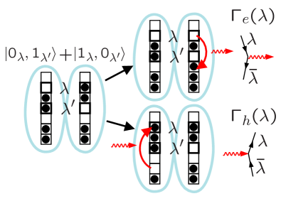
Figure 3: Sketch of two many-particle states forming a coherent superposition, and two possible scattering processes contributing to $\Gamma_{e}(\lambda)$ and $\Gamma_{h}(\lambda)$, by emission and absorption, respectively.

Below we shall also need the rate for an initially empty state $\lambda$ to be filled, i.e. the decay rate of a hole, given by:

$$\Gamma_{h}(\lambda) = {{2\pi}\over\hbar}\int_{-\infty}^{\infty}\!(d\bar{\omega})\bigl{\langle}\hat{V}\hat{V}\bigr{\rangle}_{\bar{\omega}}\,f(\varepsilon_{\lambda}+\bar{\omega})D(\varepsilon_{\lambda}+\bar{\omega})\qquad\phantom{.}$$

$$= \int_{0}^{\infty}\!(d\bar{\omega})\,2\textrm{Im}\bar{\cal L}^{R}(\bar{\omega})\Bigl{\{}\bigl{[}1+n(\bar{\omega})\bigr{]}\,f(\varepsilon_{\lambda}+\bar{\omega})\Bigr{.}$$

$$\Bigl{.}\times D(\varepsilon_{\lambda}+\bar{\omega})+n(\bar{\omega})\,f(\varepsilon_{\lambda}-\bar{\omega})\,D(\varepsilon_{\lambda}-\bar{\omega})\Bigr{\}}\,.$$

In the second equality, the first and second terms describe emission and absorption processes, whereby an electron from a higher- or lower-lying level is scattered into the empty hole level $\lambda$, respectively. Again we see that at $T=0$, only spontaneous emission is possible, and if $\varepsilon_{\lambda}\rightarrow 0$, this process is suppressed, too.

V.3 Golden rule decay rates for coherent superpositions

In order to calculate the decoherence rate, we have to consider a somewhat more complicated situation. Suppose we are interested in the linear response of the system to some perturbation (as is the case for the conductivity calculation in the weak localization problem). If the perturbation scatters an electron from level $\lambda$ to level $\lambda^{\prime}$, then the resulting state is of the form $(1+\epsilon\psi_{\lambda^{\prime}}^{\dagger}\hat{\psi}_{\lambda})\bigl{|}\Phi\bigr{\rangle}$, where $\epsilon\ll 1$ is small. Contributions of this type can occur if $\bigl{|}\Phi\bigr{\rangle}$ has one electron in $\lambda$ but none in $\lambda^{\prime}$; apart from this restriction, $\bigl{|}\Phi\bigr{\rangle}$ is some Slater determinant with arbitrary distribution of fermions over the other single-particle levels, and we will perform a thermal average over such states in the end. Effectively, we have thus created a coherent superposition of two many-particle states, which, for brevity, we shall call $\bigl{|}1_{\lambda},0_{\lambda^{\prime}}\bigr{\rangle}+\epsilon\bigl{|}0_{\lambda},1_{\lambda^{\prime}}\bigr{\rangle}$. These are formed from an initial state with unoccupied $\lambda$ and $\lambda^{\prime}$ by inserting a single extra particle into a coherent superposition $c^{\dagger}_{\lambda}+\epsilon c^{\dagger}_{\lambda^{\prime}}$ of these two levels (Fig. 3). Our task is to calculate the decay rate of this coherent superposition, which under appropriate assumptions (discussed below) corresponds to the “decoherence rate”. Although we shall eventually need only the case $\varepsilon_{\lambda}=\varepsilon_{\lambda^{\prime}}$ (see Ref. wneq0, ), we shall for clarity distinguish the indices $\lambda$ and $\lambda^{\prime}$ througout this subsection.

The coherent superposition will be destroyed by any process that leads to a decay of one or the other many-particle state. This includes not only an electron leaving $\lambda$ or $\lambda^{\prime}$, but also an electron entering the respective unoccupied state ($\lambda^{\prime}$ or $\lambda$). The total decay rate for the coherent superposition therefore is the sum of four contributions (after thermal averaging over the electron distribution):

$$\Gamma_{\varphi}(\lambda,\lambda^{\prime})={\textstyle\frac{1}{2}}\Big{[}\Gamma_{e}(\lambda)+\Gamma_{h}(\lambda^{\prime})+\Gamma_{e}(\lambda^{\prime})+\Gamma_{h}(\lambda)\Bigr{]}\,.$$ (70)

The first two terms give the decay rate for the state $\bigl{|}1_{\lambda},0_{\lambda^{\prime}}\bigr{\rangle}$, while the latter two refer to $\bigl{|}0_{\lambda},1_{\lambda^{\prime}}\bigr{\rangle}$. The factor ${\textstyle\frac{1}{2}}$ comes about because decoherence is due to the decay of wave functions rather than populations (the same is seen in usual master equation formulations of decoherence of systems with a discrete Hilbert space).

In writing down Eq. (70), we have assumed that all of the decay processes lead to decoherence. However, one may think of situations where Eq. (70) would overestimate the decoherence rate: For example, an electron traveling two different paths may scatter a phonon on both of these paths (similar to decay processes making the electron leave $\lambda$ and $\lambda^{\prime}$). But the interference is destroyed only if the wavelength of the phonon is sufficiently short to be able to distinguish the two paths from each other, since otherwise the information about the path of the electron is not revealed in the scattering process. In fact, disregarding this possibility amounts to neglecting vertex corrections in the diagrammatic calculation. Whether such an approximation is justified depends (among other things) on the operator whose expectation value is to be calculated in the end. This operator should connect the two states $\bigl{|}1_{\lambda},0_{\lambda^{\prime}}\bigr{\rangle}$ and $\bigl{|}0_{\lambda},1_{\lambda^{\prime}}\bigr{\rangle}$, in order to be sensitive to the coherence of the state. It is necessary to specify this operator for each particular microscopic model, as well as the operator of the initial perturbation and the details of the system-bath coupling. However, such details are not important in the present section, since our aim here is merely to display the simple generic features of the golden rule decoherence rate in a fermion system.

It is illuminating to relate the calculation presented above to the decay of the single-particle retarded Green’s function, $G_{\lambda}^{R}(t)$, which appears in diagrammatic calculations. According to the definition of $G^{R}_{\lambda}$, we have to consider the decay of the following overlaps:

$$i{\hbar}G_{\lambda}^{R}(t) \equiv \theta(t)\bigl{\langle}\bigl{\{}\hat{\psi}_{\lambda}(t),\hat{\psi}_{\lambda}^{\dagger}(0)\bigr{\}}\bigr{\rangle}$$ (71)

$$= \theta(t)\left[\bigl{\langle}\hat{\psi}_{\lambda}^{\dagger}\hat{U}(t)\Phi_{0}\bigl{|}\hat{U}(t)\hat{\psi}_{\lambda}^{\dagger}\Phi_{0}\bigr{.}\rangle\right.$$

$$\left.+\bigl{\langle}\hat{U}(t)\hat{\psi}_{\lambda}\Phi_{0}\bigl{|}\hat{\psi}_{\lambda}\hat{U}(t)\Phi_{0}\bigr{.}\bigr{\rangle}\right],$$

where $\bigl{|}\Phi_{0}\bigr{\rangle}$ denotes the ground state at $T=0$ (or some state over which a thermal average is to be performed). Here $\hat{U}(t)$ is the full time evolution operator, including the coupling to the environment. The first overlap can decay by two processes: Either the ket-state changes during the time $t$ by the particle leaving the initial level $\lambda$, or the bra-state changes by a particle entering $\lambda$ (before the time $t$). Thus, the decay rate for the first term is

$$\Gamma_{e}(\lambda)+\Gamma_{h}(\lambda)={{2\pi}\over\hbar}\int_{-\infty}^{\infty}(d\bar{\omega})\,\textrm{Im}\bar{\cal L}^{R}(\bar{\omega})\times$$

$$\left[\coth\Bigl{(}\frac{\bar{\omega}}{2T}\Bigr{)}+\tanh\Bigl{(}\frac{\varepsilon_{\lambda}-\bar{\omega}}{2T}\Bigr{)}\right]D(\varepsilon_{\lambda}-\bar{\omega})\,.$$ (72)

By similar reasoning, the decay rate for the second term of Eq. (71) is given by the same expression. Note in particular that a combination “$\coth+\tanh$” arises Eq. (72); this combination is well known from diagrammatic calculations of the decoherence rate in weak localization (see e.g. Ref. Abrahams, ). At large positive energy transfers $\bar{\omega}\gg\varepsilon_{\lambda},\,T$ (emission of energy into the environment), this factor vanishes, due to the Pauli blocking of final states. Likewise, large negative energy transfers (absorption of energy) are also forbidden, because the environment does not contain thermal quanta needed for that process.

Likewise, the decay rate of $G_{\lambda^{\prime}}^{A}(t)$ is found to be $\Gamma_{e}(\lambda^{\prime})+\Gamma_{h}(\lambda^{\prime})$. Thus, (in the absence of vertex corrections) the decay rate for $G_{\lambda}^{R}G_{\lambda^{\prime}}^{A}$ coincides with the total decoherence rate $\Gamma_{\varphi}(\lambda,\lambda^{\prime})$ of Eq. (70), as expected. For the purpose of calculating the decoherence rate, for which we need the long-time behavior of the Cooperon ${\tilde{C}}(0,t)$ for $Tt\gg 1$, it suffices to take the electron and hole energies equalwneq0 , $\varepsilon_{\lambda}=\varepsilon_{\lambda^{\prime}}$, which will be done henceforth.

In a related context, an explicit (non-diagrammatic) calculation of the decoherence rate has been performed for a fermionic ballistic Mach-Zehnder interferometer. This calculation is devoid of the complications introduced by impurity averaging but displays all the features regarding the Pauli principle which have been discussed hereMachZehnder .

V.4 Pauli-blocked noise correlator $\bigl{\langle}\hat{V}\hat{V}\bigr{\rangle}^{\rm\textrm{pp}}_{{\bar{q}}\bar{\omega}}$

The discussion of decoherence and weak localization in Section III had been purposefully restricted to situations where the Pauli principle played no role; in a many-body situation, this corresponds e.g. to a highly excited electron state, with $\varepsilon_{\lambda}$ so large that $f(\varepsilon_{\lambda}\pm\bar{\omega})=0$. Taking the density of states $D(\varepsilon)$ to be constant henceforth, we then note from Eqs. (LABEL:eq:Gammael-a) and (V.2) that for $f=0$ the decoherence rate calculated in the previous subsection indeed depends on the symmetrized correlator only,

$$\Gamma_{e}(\lambda)+\Gamma_{h}(\lambda)\propto\int_{-\infty}^{\infty}(d\bar{\omega})\,{\textstyle\frac{1}{2}}\bigl{\langle}\{\hat{V},\hat{V}\}\bigr{\rangle}_{\bar{\omega}}\;,$$ (73)

in agreement with the conclusion of Eqs. (57) and (58).

Moreover, we observe from Eqs. (LABEL:eq:Gammael-a) and (V.2) that in the present context, “switching on” the Pauli principle (i.e. permitting $f\neq 0$) amounts to replacing ${\textstyle\frac{1}{2}}\bigl{\langle}\{\hat{V},\hat{V}\}\bigr{\rangle}_{\bar{\omega}}$ in Eq. (73) by

$${\textstyle\frac{1}{2}}\bigl{\langle}\{\hat{V},\hat{V}\}\bigr{\rangle}_{\bar{\omega}}+\bigl{[}f(\varepsilon_{\lambda}+\bar{\omega})-f(\varepsilon_{\lambda}-\bar{\omega})\bigr{]}{\textstyle\frac{1}{2}}\bigl{\langle}[\hat{V},\hat{V}]\bigr{\rangle}_{\bar{\omega}}.\;$$ (74)

This yields a “Pauli-blocked” noise spectrum [compared to Eq. (58)], which is, however, still symmetric and non-negative.

Now, since the decay functions $F(t)$ discussed in earlier sections and the golden rule analysis presented above are both linear in the interaction propagator, the lessons learnt from the golden rule about Pauli blocking should be directly relevant for $F(t)$, too. Thus, we formulate the following hypothesis: if the first-order correction to the Cooperon $\tilde{C}^{1}$ were calculated by a proper many-body technique, the result for $F(t)=-{\tilde{C}}^{1}(0,t)/{\tilde{C}}^{0}(0,t)$ will have the same form as Eq. (57),

$$F^{\textrm{pp}}_{d}(t) = {1\over\hbar^{2}}\int_{-{t\over 2}}^{{t\over 2}}dt_{3}\int_{-{t\over 2}}^{{t\over 2}}dt_{4}\,\int(d\bar{q})\int(d\bar{\omega})\,e^{-i\bar{\omega}t_{34}}$$ (75)

$$\times\bigl{\langle}VV\bigr{\rangle}_{{\bar{q}}\bar{\omega}}^{\textrm{pp}}\>\,\delta{\bar{P}}({\bar{q}};\tau_{34},{\widetilde{\tau}}_{34})\;,$$

except that the effective noise spectral function now has the following form, modified by the Pauli principle (pp):

$$\bigl{\langle}VV\bigr{\rangle}^{\textrm{eff}}_{{\bar{q}}\bar{\omega}}\mapsto\bigl{\langle}VV\bigr{\rangle}^{\textrm{pp}}_{{\bar{q}}\bar{\omega}}$$ (76b)

$$\phantom{.}\equiv{\textstyle\frac{1}{2}}\bigl{\langle}\{V,V\}\bigr{\rangle}_{{\bar{q}}\bar{\omega}}+\bigl{[}f(\varepsilon+\bar{\omega})-f(\varepsilon-\bar{\omega})\bigr{]}{\textstyle\frac{1}{2}}\bigl{\langle}[\hat{V},\hat{V}]\bigr{\rangle}_{{\bar{q}}\bar{\omega}}\,$$

$$\phantom{.}={\hbar}\,\textrm{Im}\bar{\mathcal{L}}_{{\bar{q}}}^{R}(\bar{\omega})\Bigl{\{}\coth\Bigl{[}{{\bar{\omega}}\over 2T}\Bigr{]}\,+{\textstyle\frac{1}{2}}(\textrm{th}_{-}-\textrm{th}_{+})\Bigr{\}}.\qquad\phantom{.}$$

Here $\varepsilon$ is the initial energy with which an electron starts off on its diffusive trajectory, and $\textrm{th}_{\pm}\equiv{\tanh[(\varepsilon\pm\bar{\omega})/2T]}$. The combination “$\coth+\tanh$” arising in Eq. (76b) is well known from diagrammatic calculations of the decoherence rate in weak localization (see e.g. Ref. Abrahams, ).

For the case of quantum Nyquist noise [Eq. (54)], ${1\over\hbar}\langle VV\rangle^{\textrm{pp}}_{{\bar{q}}\bar{\omega}}$ can be written in the factorized form ${\mathcal{W}}_{\textrm{pp}}(\bar{\omega})/\nu D{\bar{q}}^{2}$ of Eq. (39), with a corresponding Pauli-principle-modified spectrum,

$${\mathcal{W}}_{\textrm{pp}}({\bar{\omega}}) = {|{\bar{\omega}}|\over 2}\Bigl{\{}2n(|\bar{\omega}|)+1+f(\varepsilon+|\bar{\omega}|)-f(\varepsilon-|\bar{\omega}|)\Bigr{\}},$$

shown in Fig. 4.

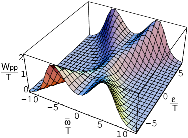
Figure 4: The spectrum ${\mathcal{W}}_{\textrm{pp}}(\bar{\omega})$ of Eq. (LABEL:eq:weightingpp) as a function of frequency and electron energy. It has the properties ${\mathcal{W}}_{p}p(0)=1$, ${\mathcal{W}}_{\textrm{pp}}\to 0$ for $\bar{\omega}\gg\max\{T,\varepsilon\}$, and in the limit $T\to 0$, behaves as ${\textstyle\frac{1}{2}}|\bar{\omega}|\theta(|\varepsilon|-|\bar{\omega}|)$.

It has the very important property that it cuts off the contribution of all frequencies $|{\bar{\omega}}|\gtrsim\max\{T,\varepsilon\}$. In particular, for an electron at the Fermi surface $(\varepsilon=0)$, the factor in curly brackets reduces to the combination $2n(|\bar{\omega}|)+2f(|\bar{\omega}|)$ anticipated by Chakravarty and Schmid [Eq. (67)], cutting off all frequencies $|{\bar{\omega}}|\gtrsim T$. At $T=0$, the spectrum ${\mathcal{W}}_{\textrm{pp}}({\bar{\omega}})$ reduces to ${\textstyle\frac{1}{2}}|\bar{\omega}|\theta(|\varepsilon|-|\bar{\omega}|)$. Moreover, at $\varepsilon=0$ and $T=0$, it yields $\{0+1+0-1\}=0$, i.e. the new Pauli terms precisely cancel the spontaneous emission term discussed in Section IV.4, as announced at the beginning of Section V. Thus, this spectrum can be expected to lead to a decoherence rate that vanishes for sufficiently small temperatures. We shall see below that this is indeed the case.

The hypothesis that the use of $\langle\hat{V}\hat{V}\rangle^{\textrm{pp}}_{{\bar{q}}\bar{\omega}}$ in our formula for $F(t)$ is the appropriate way to incorporate the Pauli principle into an influence functional approach will be shown to be correct in subsequent parts of this work: In Section VII.1, this replacement will be justified within the context of the functional integral analysis of decoherence of Ref. vonDelft04, . Moreover, the Bethe-Salpeter analysis of paper II likewise turns out to lead to a decay function [Eq. (II.LABEL:eq:exponentBetheSalpeter)] involving precisely the Pauli-principle-modified weighting function of Eq. (76); in particular, the diagrammatic calculation of ${\tilde{C}}^{1}(0,t)$ performed there confirms explicitly that $F(t)^{\textrm{pp}}_{d}=-{\tilde{C}}^{1}(0,t)/{\tilde{C}}^{0}(0,t)$.

VI Results for Decay Function $F_{d}^{\textrm{pp}}(t)$

VI.1 Energy-averaged Decay Function $\langle F_{d}^{\textrm{pp}}(t)\rangle_{\varepsilon}$

Since the correlator $\langle VV\rangle^{\textrm{pp}}_{{\bar{q}}\bar{\omega}}$ occuring in $F^{\textrm{pp}}(t)$ depends on the initial energy $\varepsilon$ with which an electron starts off on its diffusive trajectory, an average of the function $e^{-F^{\textrm{pp}}_{d}(t)}$ over this energy still has to be performed, using the usual derivative of the Fermi function:

$$\langle...\rangle_{\varepsilon}\equiv\int d\varepsilon[-f^{\prime}(\varepsilon)]\>...\;.$$ (78)

We shall simplify the calculation by lifting the energy average into the exponent:

$$\left\langle e^{-F_{d}^{\textrm{pp}}(t)}\right\rangle_{\varepsilon}\simeq e^{-\langle F^{\textrm{pp}}_{d}(t)\rangle_{\varepsilon}}\;,$$ (79)

thereby again somewhat overestimating the actual decoherence rate [cf. discussion after Eq. (28)]. The energy average of the decay function, $F^{\overline{\textrm{pp}}\hskip 1.13809pt}_{d}(t)\equiv\langle F^{\textrm{pp}}_{d}(t)\rangle_{\varepsilon}$, has the same form as Eq. (75), but now with an energy-averaged spectrum:

$${\mathcal{W}}_{\overline{\textrm{pp}}\hskip 1.13809pt}({\bar{\omega}})\equiv\bigl{\langle}{\mathcal{W}}_{\textrm{pp}}({\bar{\omega}})\bigr{\rangle}_{\varepsilon} = T\left({\bar{\omega}/2T\over\sinh[\bar{\omega}/2T]}\right)^{2}\;,\qquad\phantom{.}$$ (80)

which exponentially suppresses the contribution of all frequencies $|{\bar{\omega}}|\gtrsim T$, as anticipated above. The fact that ${\mathcal{W}}_{\overline{\textrm{pp}}\hskip 1.13809pt}({\bar{\omega}})\leq{\mathcal{W}}_{\textrm{cl}}({\bar{\omega}})=T$ for all frequencies, but in particular for ${\bar{\omega}}\gtrsim T$, implies that the effective energy-averaged Pauli-blocked noise is somewhat less noisy than classical noise; thus, the decoherence times for the former can be expected to be somewhat longer than for the latter, as will indeed be found below.

Evaluating the Fourier transform of ${\mathcal{W}}_{\overline{\textrm{pp}}\hskip 1.13809pt}({\bar{\omega}})$ (by closing the $\int d{\bar{\omega}}$-integral in Eq. (41) along a semicircular path in the complex plane), we find the kernel

$$W_{\overline{\textrm{pp}}\hskip 1.13809pt}(t_{34})=\pi T^{2}w(\pi Tt_{34}),\;\quad w(z)={z\coth z-1\over\sinh^{2}z}\;,\quad\phantom{.}$$ (81)

where $w(z)$ is a positive, peak-shaped function with weight $\int_{-\infty}^{\infty}dz\,w(z)=1$. Thus, $W_{\overline{\textrm{pp}}\hskip 1.13809pt}(t_{34})$ equals $T$ times a broadened delta function of width $1/T$, and in the limit $T\to\infty$, we recover $W_{\overline{\textrm{pp}}\hskip 1.13809pt}(t_{34})\to W_{\textrm{cl}}(t_{34})$. Inserting Eq. (81) into Eq. (43), we obtain

$$F^{\overline{\textrm{pp}}\hskip 1.13809pt}_{d}(t)={Tt\over g_{d}(L_{t})}\int_{0}^{\pi Tt}\!\!dz\,w(z)\,{{\cal P}}_{d}^{\textrm{crw}}\left({z\over\pi Tt}\right)\;.\qquad\phantom{.}$$ (82)

Since the decoherence time is defined by asking when $F({\tau_{\varphi}})={\cal O}(1)$, and $g_{d}(L_{\varphi})\gg 1$ [cf. discussion after Eq. (22)], Eq. (82) implies that $T{\tau_{\varphi}}\gg 1$. Thus, to determine $F(t)$ for times $t\simeq{\tau_{\varphi}}$, we may take the limit $Tt\gg 1$ in Eq. (82), obtaining for the leading and next-to-leading terms:

$$F^{\overline{\textrm{pp}}\hskip 1.13809pt}_{1}(t) = {Tt\over g_{1}(L_{t})}\left[c_{1}-{b_{1}\over\sqrt{Tt}}\right]\;,$$ (83a)

$$F^{\overline{\textrm{pp}}\hskip 1.13809pt}_{2}(t) = {Tt\over g_{2}(L_{t})}\bigl{[}c_{2}\ln(Tt)-b_{2}\bigr{]}\;,$$ (83b)

$$F^{\overline{\textrm{pp}}\hskip 1.13809pt}_{3}(t) = {(Tt)^{3/2}\over g_{3}(L_{t})}\left[c_{3}-{b_{3}\over\sqrt{Tt}}\right]\;.$$ (83c)

Here the prefactors $c_{1}^{\textrm{crw}}$ and $c_{1}^{\textrm{urw}}$ are the same as in Eq. (50), reproducing the results obtained there for classical white Nyquist noise. The prefactors $c_{2}=1/(2\pi)$ and $c_{3}=\int_{0}^{\infty}dz\,w(z)/(\pi\sqrt{z})={3\zeta(3/2)/\sqrt{\pi^{3}2^{5}}}=0.2488$ are independent of whether the average over paths is performed over closed or unrestricted random walks, because the same is true for the leading terms of ${{\cal P}}_{2}$ and ${{\cal P}}_{3}$ in Eqs. (44). Hence, in contrast to $d=1$, averaging over closed instead of unrestricted random walks yields no increase in accuracy for the leading terms of $F_{d}^{\overline{\textrm{pp}}\hskip 1.13809pt}(t)$ for $d=2$ and 3. It does make a difference for the subleading terms, for which we find $b_{1}^{\textrm{crw}}=b_{1}^{\textrm{urw}}=(2\pi)^{-1/2}\,|\zeta({\textstyle\frac{1}{2}})|=0.5826$, $b_{2}^{\textrm{crw}}=(1-\gamma_{\rm Euler})/(2\pi)=0.06729$, $b_{2}^{\textrm{urw}}=-\gamma_{\rm Euler}/(2\pi)=-0.09187$, $b_{3}^{\textrm{crw}}={\textstyle\frac{1}{2}}\pi^{-1/2}$, $b_{3}^{\textrm{urw}}=\pi^{-3/2}$.

For unrestricted random walks, the leading terms of $F_{d,\textrm{urw}}^{\overline{\textrm{pp}}\hskip 1.13809pt}(t)$ can also be obtained with remarkable ease from its frequency representation (45): replacing ${\mathcal{W}}_{\textrm{eff}}(\bar{\omega})$ by ${\mathcal{W}}_{\overline{\textrm{pp}}\hskip 1.13809pt}(\bar{\omega})$ and evaluating the leading contributions to the integral in the limit $Tt\gg 1$, one readily recovers the leading terms of Eqs. (83) [including the correct prefactors $c_{d}$].

Let us now calculate the full decoherence times ${\widetilde{\tau}}_{\varphi,d}$ (including next-to-leading order corrections). For $t\simeq{\widetilde{\tau}}_{\varphi,d}$, the next-to-leading terms in Eqs. (83) are parametrically parametrically smaller than the leading ones by $g^{-1/2}_{1}(L_{\varphi,1})$ for $d=1$, or $1/\ln g_{2}$ for $d=2$, or $g^{-1/3}_{3}(L_{\varphi,3})$ for $d=3$. Therefore, we write ${\widetilde{\tau}}_{\varphi,d}=\tau_{\varphi,d}(1+\delta_{d})$, where $\delta_{d}\ll 1$ is a small correction induced by the next-to-leading terms, and first determine $\tau_{\varphi,d}$, by setting $b_{d}\to 0$ and $\delta_{d}\to 0$. Then the conditionthresholdconstant $F_{d}^{\overline{\textrm{pp}}\hskip 1.13809pt}(\tau_{\varphi,d})=1$ yields the the following selfconsistency relations and solutions,

$$\gamma_{\varphi,1} = {c_{1}T\over g_{1}(L_{\varphi,1})}\;\qquad\,\Rightarrow\;\gamma_{\varphi,1}=(c_{1}\sqrt{\gamma_{1}}\,T)^{2/3}\!\!,\qquad\phantom{.}$$ (84a)

$$\gamma_{\varphi,2} = {c_{2}T\ln\left(T\tau_{\varphi,2}\right)\over g_{2}(L_{\varphi,2})}\;\Rightarrow\;\gamma_{\varphi,2}={c_{2}T\over g_{2}}\ln(g_{2}/c_{2})\;,\qquad\phantom{.}$$ (84b)

$$\gamma_{\varphi,3} = {c_{3}T\over g_{3}(L_{T})}\quad\qquad\Rightarrow\;\gamma_{\varphi,3}={c_{3}T^{3/2}\over\sqrt{\gamma_{3}}}\;,$$ (84c)

where $\gamma_{1},g_{2},\gamma_{3}$ are defined in Eq. (11), and $L_{T}=\sqrt{D/T}$. These results reproduce those first derived by AAK for classical white Nyquist noise. They can be used to write the decay functions $F_{d}^{\overline{\textrm{pp}}\hskip 1.13809pt}(t)$ in the form (16) cited in the overview [Sec. II.4].

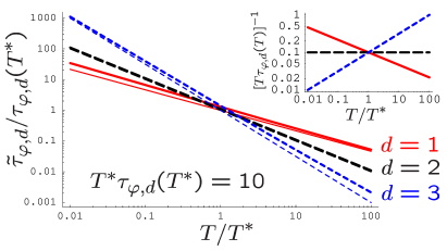
Figure 5: Comparison of the commonly employed leading approximation for the decoherence time ${\tau}_{\varphi,d}$ (thin lines) and the full decoherence time ${\tilde{\tau}}_{\varphi,d}$ (thick lines), as a function of temperature, for dimensions $d=1$ (full red lines), $d=2$ (black, long dashed), $d=3$ (blue, short dashed). The temperature $T^{*}$ has been (arbitrarily) chosen to give $T^{*}{\tau}_{\varphi,d}(T^{*})=10$ in all cases (this amounts to fixing the values of the material parameters $\gamma_{1}$, $g_{2}$ and $\gamma_{3}$). The magnitude of the correction is governed by the small parameter $[T\tau_{\varphi,d}]^{-1}$, who’s $T$-dependence is shown in the inset: In $d=1$ ($d=3$) the corrections become smaller (and the weak localization theory is applicable) towards higher (lower) temperatures, where $[T{\tau}_{\varphi,d}(T)]^{-1}\ll 1$. In $d=2$, the correction amounts to a numerical constant factor (shift on the log-scale, hardly visible in this figure). Note, in particular, the slow decay of the correction in the case of $d=1$, where the correction falls off only like $T^{-1/6}$ [compare Eqs. (84) and (85)].

Next we work out the corrections to the decoherence times due to the next-to-leading terms in Eqs. (83). Reinstating $b_{d}\neq 0$ and solving the condition $F_{d}^{\overline{\textrm{pp}}\hskip 1.13809pt}({\widetilde{\tau}}_{\varphi,d})=1$ for $\delta_{d}(\tau_{\varphi,d})$, we find

$$\delta_{1} = {2\over 3}{b_{1}/c_{1}\over\sqrt{T\tau_{\varphi,1}}}\;,\quad\delta_{2}={b_{2}/c_{2}\over\ln(T\tau_{\varphi,2})}\;,\quad\delta_{3}={b_{3}/c_{3}\over\sqrt{T\tau_{\varphi,3}}}\;,$$

leading to Eqs. (17) for ${\widetilde{\tau}}_{\varphi,d}$. As anticipated above, the correction factors $\delta_{d}$ are parametrically small, being of order $g^{-1/2}_{1}(L_{\varphi,1})$ for $d=1$, or $1/\ln g_{2}$ for $d=2$, or $g^{-1/3}_{3}(L_{\varphi,3})$ for $d=3$. We thus arrive at the most important conclusion of this paper: the leading quantum corrections to the classical results for the decoherence rates and decay functions are parametrically small in the regime where weak localization theory is applicable. (The same qualitative conclusion was arrived at by Vavilov and AmbegaokarAV several years ago by somewhat more indirect means). Nevertheless, note that the next-to-leading corrections are still parametrically larger than all futher subleading corrections, that could arise, e.g., from calculating $F_{d}^{\overline{\textrm{pp}}\hskip 1.13809pt}(t)$ to second order in the interaction propagator, or from including crossterms between weak localization and interaction corrections (as considered diagrammatically in LABEL:AAG), since such corrections are all smaller than the leading ones by at least $1/g_{d}(L_{\varphi})$. The leading and next-to-leading approximations to the decoherence times are plotted for all three dimensions in Fig. 5. As it is not uncommon for weak localization experiments to reach to the regime where the product $T\tau_{\varphi}$ is only on the order of $10$ (e.g. Ref. Pierre03, ), we emphasize that the corrections discussed here can amount to an appreciable effect. We also remark that, in $d=1$, the relative size of the correction only falls off very slowly with increasing temperature (like $T^{-1/6}$).

The temperature dependence predicted for the corrected decoherence times ${\widetilde{\tau}}_{\varphi,d}(T)$ can be compared to experiment by proceeding as follows: Express $F_{d}(t)$ of Eqs. (83) as a function of the parameters $(t/{\widetilde{\tau}}_{\varphi,d})$ and $T{\widetilde{\tau}}_{\varphi,d}$, by inserting $\tau_{\varphi,d}={\widetilde{\tau}}_{\varphi,d}[1-\delta_{d}({\widetilde{\tau}}_{\varphi,d})]$. Calculate the magnetoconductivity $\sigma^{\rm WL}_{d}(H)$ numerically from Eq. (22), and for given $T$, adjust the parameter ${\widetilde{\tau}}_{\varphi,d}$ such that the numerical curve as a function of magnetic field best fits the measured curve. Repeat for various $T$, and compare the function ${\widetilde{\tau}}_{\varphi,d}(T)$ obtained by this fitting procedure to the function $\tau_{\varphi,d}(1+\delta_{d})$ predicted above. [If magnetic impurities are suspected to be present, insert a factor $e^{-t/\tau_{{\rm m}}}$ into Eq. (22) and treat the magnetic scattering time $\tau_{\rm m}$ as a fit parameter. Spin-orbit scattering is not included in our analysis, but the corresponding generalization should be straightforward.]

To end this section, some remarks on the role of an ultraviolet cutoff seem to be in order at this point: for quantum noise in the absence of Pauli blocking, an ultraviolet cutoff always has to be introduced to arrive at a finite result for the decoherence rate, to reqularize the contribution of spontaneous emission processes which occur at all frequencies (see our discussion in Sec. IV.4). In the full theory, Pauli blocking counteracts spontaneous emission and introduces via ${\mathcal{W}}_{\overline{\textrm{pp}}\hskip 1.13809pt}(\bar{\omega})$ an effective ultraviolet cutoff at frequency transfers of order $T$. Remarkably, for $d=1$ (but not for $d=2,3$), the leading result for the decoherence rate can nevertheless be correctly obtained by simply employing the classical white noise spectrum ${\mathcal{W}}_{\textrm{cl}}(\bar{\omega})=T$ (which contains no Pauli blocking, but no spontaneous emission either ) over the full frequency range up to arbitrary frequencies. The reason is that for $d=1$, the dominant contribution to decoherence for time-reversed diffusive paths of duration $t$ comes from frequencies $\bar{\omega}\sim D{\bar{q}}^{2}\sim 1/t$ [cf. Eq. (42)], which in the limit $1\ll Tt$ of present interest implies $\bar{\omega}\ll T$; but for these frequencies, the spectrum ${\mathcal{W}}_{\textrm{pp}}(\bar{\omega})$ reduces simply to $T$, which equals the classical spectrum ${\mathcal{W}}_{\textrm{cl}}(\bar{\omega})$.

In contrast, for $d=2,3$ the large-frequency regime makes a logarithmic contribution for $d=2$, and dominates for $d=3$, requiring an ultraviolet cutoff to be present in the theory. AAK had to introduce such an ultraviolet cutoff by hand for the cases $d=2,3$, because they considered only classical white Nyquist noise, whose instantaneous kernel $W_{\textrm{cl}}(t_{34})=T\delta(t_{34})$ involves no upper frequency cutoff, which is unphysical. Indeed, when one attempts to use it in Eq. (43), the $\int dt_{34}$ integral would be ill-defined, since the $\delta(t_{34})$ would produce a $\ln(0)$ or $1/\sqrt{0}$ in ${{\cal P}}_{2}$ or ${{\cal P}}_{3}$ of Eqs. (44), respectively. Equivalently, using ${\mathcal{W}}_{\textrm{cl}}(\bar{\omega})=T$ in Eq. (45), the frequency integral would be ultraviolet-divergent for $d=2,3$. AAK cured this problem by introducing, by hand, an ultraviolet cutoff at the scale of the temperature (taking $|{\bar{q}}|\lesssim\sqrt{T/D}$), and adding, by hand, a term to the decoherence rate describing the effect of electron-electron collisions with large energy transfers $\bar{\omega}\gtrsim T$, which had been calculated earlier AltshulerAronov81 within the framework of a kinetic equation. (GZ’s work implicitly questions this approach, in that they used $1/{\tau_{\textrm{el}}}\;(\gg T)$ as upper cutoff.)

Satisfactorily, an ultraviolet cutoff of precisely the type used by AAK arises automatically in our treatment of quantum Nyquist noise in combination with the Pauli principle, in the form of the energy-averaged spectrum ${\mathcal{W}}_{\overline{\textrm{pp}}\hskip 1.13809pt}(\bar{\omega})$: it regularizes the large-frequency behavior of Eq. (45), without the need to consider processes with large energy transfers separately. Equivalently, in the time domain, it results in $W_{\overline{\textrm{pp}}\hskip 1.13809pt}(t_{34})$ being a broadened $\delta(t_{34})$-function of width $1/T$. Thus, in a very natural (and perhaps somewhat more elegant) manner, we have confirmed the validity of AAK’s use of temperature as an ultraviolet cutoff. Moreover, our explicit treatment of this cutoff was essential for accurately calculating the next-to-leading terms for the decay function and decoherence times.

VI.2 Comparison with Magnetoconductivity of AAG

It is instructive to check the use of the Pauli-blocked correlator $\bigl{\langle}\hat{V}\hat{V}\bigr{\rangle}^{\textrm{pp}}_{{\bar{q}}\bar{\omega}}$ introduced above against the results of Ref. AAG, (AAG). There, the conductivity was calculated diagrammatically for the limit of a moderately strong magnetic field (for ${\gamma_{\varphi}}\ll{\gamma_{H}}\ll T$). In this regime the trajectories relevant for weak localization are so short ($t\lesssim{\tau_{H}}\ll{\tau_{\varphi}}$) that the effects of interaction on weak localization are still small, so that it suffices to calculate $\delta\sigma^{\rm WL}_{d}$ to first order in the interaction. At the same time, the condition $1/T\ll{\tau_{H}}$ ensures that the premise for our calculations of ${\tau_{\varphi}}$ in previous sections, namely $1/T\ll{\tau_{\varphi}}$, still holds. AAG thus calculated the conductivity diagrammatically to first order in the interaction and including all contributions of order $1/g^{2}$ (including not only weak localization terms, but also interaction corrections and cross terms involving both). Among these $1/g^{2}$ terms, AAK identified the one that decreases most rapidly with magnetic field (largest power of ${\tau_{H}}$) as the one relevant for decoherence, and proposed to extract ${\tau_{\varphi}}$ from it. They found that this term has the following form [Eq. (4.5) of Ref. AAK, , rewritten in terms of quantities introduced above],

$$\delta\sigma^{{\rm WL}(1)}_{d,{\scriptscriptstyle{\rm AAG}}} = -\frac{\sigma_{d}}{\pi\nu{\hbar}}\int(d\bar{\omega})(d\bar{q})(dq)\,{{2}\over\hbar^{2}}\,\Bigl{\langle}\bigl{\langle}\hat{V}\hat{V}\bigr{\rangle}_{{\bar{q}}\bar{\omega}}^{\textrm{pp}}\Bigr{\rangle}_{\varepsilon}$$

$$\times\Big{[}{\overline{\cal C}}{}^{0}_{{\bm{q}}-{\bar{\bm{q}}}}(0)\,|{\overline{\cal C}}{}^{0}_{\bm{q}}({\bar{\omega}})|^{2}\,-\,\left[{\overline{\cal C}}{}^{0}_{\bm{q}}(0)\right]^{2}\,{\overline{\cal C}}{}^{0}_{{\bm{q}}-{\bar{\bm{q}}}}({\bar{\omega}})\Bigr{]}\;.$$

AAG evaluated the integrals using dimensional regularization, finding the following resultstemp=freq [first two terms of their Eqs. (4.13)AAGtypo2 ; we also evaluate their general result (4.11) for $d=3$, sending $(3-d)^{-1}\to\ln({\tau_{H}}/{\tau_{\textrm{el}}})$ in the limit $d\to 3$, as appropriate for their dimensional regularization scheme]:

$${\delta\sigma^{{\rm WL}(1)}_{1,{\scriptscriptstyle{\rm AAG}}}\over\sigma_{1}} = {(T{\tau_{H}})^{3/2}\left[1-{|\zeta({\textstyle\frac{1}{2}})|\over\sqrt{\pi T{\tau_{H}}/2}}+\dots\right]\over 4\pi g_{1}(L_{H})g_{1}(L_{T})}\;,\qquad\phantom{.}$$ (87a)

$${\delta\sigma^{{\rm WL}(1)}_{2,{\scriptscriptstyle{\rm AAG}}}\over\sigma_{2}} = {T{\tau_{H}}\over 4\pi^{3}g^{2}_{2}}\Bigl{[}\ln(T{\tau_{H}})-1+\dots\Bigr{]}\;,$$ (87b)

$${\delta\sigma^{{\rm WL}(1)}_{3,{\scriptscriptstyle{\rm AAG}}}\over\sigma_{3}} = {T{\tau_{H}}\left[{3\zeta({3\over 2})\over(\pi^{7}2^{9})^{1/2}}-{\ln(\tau_{H}/\tau_{\rm el})\over 8\pi^{3}\sqrt{T{\tau_{H}}}}+\ldots\right]\over g_{3}(L_{H})g_{3}(L_{T})}\;.\qquad\phantom{.}$$ (87c)

Here $\dots$ indicates subleading terms with a weaker ${\tau_{H}}$-dependence. Moreover, AAG showed that the contribution from cross terms between interaction corrections and weak localization (their Eq. (4.7) for $\delta\sigma^{\scriptscriptstyle{\rm AAG}}_{\rm CWL}$) produce a ${\tau_{H}}$-dependence weaker than both the leading and next-to-leading terms of Eqs. (87).

Eq. (VI.2) can be reproduced from the analysis presented above, by calculating the magnetoconductivity using our first order expression for the Cooperon. To this end, use ${\tilde{C}}^{1,\varepsilon}=-{\tilde{C}}^{0}F^{\textrm{pp}}_{d,\textrm{crw}}$ [cf. Eq. (4a)] in Eq. (1) for the magnetoconductivity and average over $\varepsilon$:

$${\delta\sigma^{\rm WL(1)}_{d}\over\sigma_{d}} = \frac{1}{\pi\nu\hbar}\int_{\tau_{\textrm{el}}}^{\infty}dt\,\tilde{C}^{0}(0,t)\bigl{\langle}F^{\textrm{pp}}_{d,\textrm{crw}}(t)\bigr{\rangle}_{\varepsilon}\,,$$ (88a)

$$= \frac{2^{1-d}}{\pi^{1+d/2}}\int_{{{\tau_{\textrm{el}}}\over{\tau_{H}}}}^{\infty}dx\,{e^{-x}\over x^{d/2}}{\bigl{\langle}F^{\textrm{pp}}_{d,\textrm{crw}}(x{\tau_{H}})\bigr{\rangle}_{\varepsilon}\over g_{d}(L_{H})}\,\qquad\phantom{.}$$ (88b)

(where $L_{H}=\sqrt{D{\tau_{H}}}$). Now substitute Eq. (75) for $F^{\textrm{pp}}_{d,\textrm{crw}}(t)$ into Eq. (88a), represent the $\delta{\bar{P}}$ occuring therein via Eq. (36a) for closed random walks, with the ${\bar{P}}$ in Eq. (36a) standing for ${\bar{P}}^{\textrm{crw}}_{(0,t)}({\bar{q}},t_{34})$, represented by the first line of Eqs. (33); then Fourier transform the three Cooperons occuring in its numerator to the frequency domain and finally perform all time integrals [Eq. (II.LABEL:subeq:definePfull) is helpful in this regard]; the result is found to be identical to Eq. (VI.2), i.e. $\delta\sigma^{\rm WL(1)}_{d}=\sigma^{{\rm WL}(1)}_{d,{\scriptscriptstyle{\rm AAG}}}$. The same conclusion can be reached by comparing AAG and our results after all necessary integrals have been performed: inserting Eqs. (83) for $F^{\overline{\textrm{pp}}\hskip 1.13809pt}_{d}(t)$ into Eq. (88b) for $\delta\sigma^{\rm WL(1)}_{d}$ and performing the time integral, we recover precisely AAG’s results (87) for $\delta\sigma^{{\rm WL}(1)}_{d,{\scriptscriptstyle{\rm AAG}}}$. Thus, our theory is consistent with the calculation of AAG. Note, in particular, that the next-to-leading terms of AAG’s results for $\delta\sigma^{{\rm WL}(1)}_{d,{\scriptscriptstyle{\rm AAG}}}$ are also correctly reproduced in this manner; in our approach, they are generated by the subleading contributions (the $b_{d}$-terms) to our decay functions $F_{d}^{\overline{\textrm{pp}}\hskip 1.13809pt}(t)$. This is a very useful consistency check. It illustrates firstly that our calculation of the next-to-leading corrections to the decoherence rate is correct, and secondly that the latter do not contain any contributions from the cross terms between weak localization and interaction corrections (which we did not calculate).

AAG proposed to extract the decoherence times $\tau_{\varphi,d}$ from their final results for $\delta\sigma^{\rm WL(1)}_{d,{\scriptscriptstyle{\rm AAG}}}$ [Eqs. (87)]. To this end, a choice has to be made about the functional dependence on time of the full Cooperon ${\tilde{C}}(0,t)$ (which AAG did not calculate explicitly), or, in our scheme, about the shape of the decay function $F_{d}(t)$. Different choices for $F_{d}(t)$ imply different “definitions” of ${\tau_{\varphi}}$, with different functional dependencies on temperature and magnetic field. In their Eq. (3.2), AAG chose to define $1/\tau_{\varphi,d}^{\scriptscriptstyle{\rm AAG}}$ as a contribution to the “Cooperon mass” [in the sense of Eq. (II.LABEL:eq:definegammaphiagain)], which implies that they assumed simple exponential decay for the Cooperon, $e^{-t(1/{\tau_{H}}+1/\tau_{\varphi,d}^{\scriptscriptstyle{\rm AAG}})}$, thus effectively making the choice $F_{d}^{\scriptscriptstyle{\rm AAG}}(t)=t/\tau_{\varphi,d}^{\scriptscriptstyle{\rm AAG}}$. Inserting this into Eq. (88a) one finds

$${\delta\sigma^{\rm WL(1)}_{d}\over\sigma_{d}} = \frac{2^{1-d}\Gamma(2-{d\over 2})}{\pi^{1+d/2}g_{d}(L_{H})}{{\tau_{H}}\over\tau_{\varphi,d}^{\scriptscriptstyle{\rm AAG}}}\qquad\phantom{.}$$ (89)

[reproducingAAGtypo AAG’s (4.3)]. When equated to the leading terms of Eqs. (87), this yields for $d=1,2$

$$\tau_{\varphi,1}^{\scriptscriptstyle{\rm AAG}} = {2g_{1}(L_{H})\over T},\quad\ \tau_{\varphi,2}^{\scriptscriptstyle{\rm AAG}}={2\pi g_{2}\over T\ln(T{\tau_{H}})},$$ (90a)

reproducingAAGtypo AAG’s (4.9), while for $$d=3$$ we obtain

$$\tau_{\varphi,3}^{\scriptscriptstyle{\rm AAG}}={\sqrt{\pi^{3}2^{5}}\over 3\zeta({3\over 2})}\,{g_{3}(L_{T})\over T}.\quad\phantom{.}$$ (90b)

Now, for $d=3$, Eq. (90b) reproduces the classical result of AAK [Eq. (84c)]. However, for $d=1,2$ Eqs. (90a) for $\tau_{\varphi,d}^{\scriptscriptstyle{\rm AAG}}$ depend on magnetic field and hence are inconsistent with AAK’s results [Eqs. (84)] for $\tau_{\varphi,d}^{\scriptscriptstyle{\rm AAK}}$, which are magnetic-field independent, since AAK chose to define $1/{\tau_{\varphi}}$ as the decoherence rate which the Cooperon would have in the absence of a magnetic field. The reason for this inconsistency is that for $d=1,2$, the Cooperon decay is not purely exponential in time [cf. Eqs. (83)], so that the usual strategy of adding inverse decay times to determine the total decay rate of two independent decay mechanisms cannot be used (as emphasized in the paper by AAK, after Eq. (32) of LABEL:AAK).

AAK’s magnetic-field-independent results for the decoherence time can be extracted from AAG’s result for $\delta\sigma^{{\rm WL}(1)}_{d,{\scriptscriptstyle{\rm AAG}}}$ only if the correct functional form for the decay function is used. Indeed, inserting the leading terms of Eqs. (83) for $F_{1,2}^{\overline{\textrm{pp}}\hskip 1.13809pt}(t)$ into Eq. (88a), we find

$${\delta\sigma^{\rm WL(1)}_{1}\over\sigma_{1}} = {1\over g_{1}(L_{H})}{\tau_{H}^{3/2}\over(\pi\tau_{\varphi,1})^{3/2}}\;,$$ (91a)

$${\delta\sigma^{\rm WL(1)}_{2}\over\sigma_{2}} = {1\over 2\pi^{2}g_{2}}\,{{\tau_{H}}\over\tau_{\varphi,2}}{\ln(T{\tau_{H}})\over\ln(T\tau_{\varphi,2})}\;.$$ (91b)

When equated to Eqs. (87), this yields

$$\tau_{\varphi,1}=\left(T\sqrt{{\gamma_{1}}\pi}/4\right)^{-1},\quad\tau_{\varphi,2}=g_{2}/[Tc_{2}\ln(T\tau_{\varphi,2})],\quad\phantom{.}$$ (92)

implying $\gamma_{\varphi,2}={c_{2}T\over g_{2}}\ln(g_{2}/c_{2})$ and thus reproducing AAK’s results (with proper prefactors included), as given by the rightmost equations of (84).

To summarize this subsection, we conclude that, satisfyingly, our results for the decay functions $F_{d}^{\overline{\textrm{pp}}\hskip 1.13809pt}(t)$ provide a bridge between the work of AAK and AAG: they allow AAK’s results for $\tau^{{\scriptscriptstyle{\rm AAK}}}_{\varphi,d}$, obtained by treating classical white Nyquist noise nonperturbatively, thereby achieving results free from infrared problems, to be extracted from AAG’s results for $\delta\sigma^{{\rm WL}(1)}_{d,{\scriptscriptstyle{\rm AAG}}}$, obtained by treating fully quantum noise perturbatively, thereby incorporating Pauli blocking and obtaining results free from ultraviolet problems. The fact that our approach is able to make such a connection between two sets of established results, one nonperturbative but classical, the other quantum but perturbative, may be regarded as a strong indication that our method is fundamentally sound.

VI.3 Energy dependence of the decay function

Instead of averaging over the energy $\hbar\varepsilon$, it is also interesting to calculate the dependence of the decoherence rate $\gamma_{\varphi}^{\varepsilon,T}$ on both temperature and energy, as would be relevant for an electron injected into a disordered metal with a definite energy (e.g. in a geometry such as that used by Pothier et al. Pothier97 ). To the best of our knowledge, this energy-dependence has not been studied before. We shall now obtain it by analysing the energy-dependence of the decay function of Eq. (75), for the case of closed random walks.

To this end, we need the Fourier transform of the Pauli-principle-modified spectrum ${\mathcal{W}}_{\textrm{pp}}(\bar{\omega})$ of Eq. (LABEL:eq:weightingpp), which can be calculated by closing the $\int d{\bar{\omega}}$ integral [Eq. (41)] along a semicircular contour in the complex plane. The result can be written as $W_{\textrm{pp}}(t_{34})=\pi T^{2}w(\varepsilon t_{34},\pi Tt_{34})$, where

$$w(y,z) = {\cos y\cosh z+(y/z)\sin y\sinh z-1\over 2\sinh^{2}z}\;.\qquad\phantom{.}$$ (93)

Inserting this into Eq. (43) for $F(t)$ we obtain the expression

$$F^{\textrm{pp}}_{d,\textrm{crw}}(t)\! = \!\!{Tt\over g_{d}(L_{t})}\int_{0}^{\pi Tt}\!\!\!dz\,w(zx/\pi,z)\,{{\cal P}}_{d}^{\textrm{crw}}\!\left({z\over\pi Tt}\right),\qquad\phantom{.}$$ (94)

which shows that $F^{\textrm{pp}}_{d}(t)g_{d}(L_{t})$ is a function of the parameters $\pi Tt$ and $x=\varepsilon/T$, or of $\pi Tt$ and $\varepsilon t$. Fig. 6(a) shows the latter functional dependence for $d=1$.

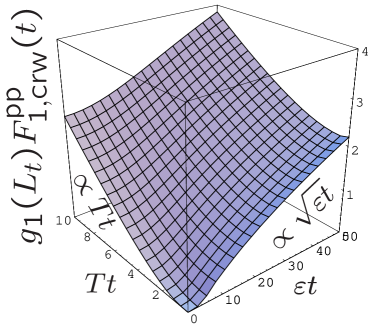
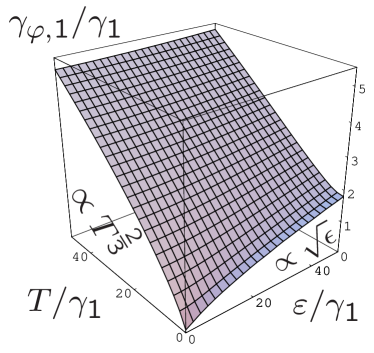
Figure 6: (a) $g_{1}(L_{t})F_{1,\textrm{crw}}^{\textrm{pp}}(t)$ [Eq. (94)] as function of the parameters $\varepsilon t$ and $Tt$. (b) The energy- and temperature-dependent decoherence rate $\tau_{\varphi,1}$, defined from the condition $F^{\textrm{pp}}_{1,\textrm{crw}}(\tau_{\varphi,1})=1$, as function of $T/{\gamma_{1}}$ and $\varepsilon/{\gamma_{1}}$.

Moreover, Fig. 6(b) shows the corresponding energy- and temperature-dependent decoherence rate $\tau_{\varphi,1}$, defined from the usual condition $F^{\textrm{pp}}_{1,\textrm{crw}}(\tau_{\varphi,1})=1$.

To extract the decoherence rate analytically from $F_{d}^{\textrm{pp}}(t)$, we need its asymptotic behavior for large times. We find that the dominant behavior of $F_{d}(t)$ for either $Tt\gg 1$ or $\varepsilon t\gg 1$ (or both), but arbitrary ratios of $\varepsilon/T$, is given by the following expressions:

$$F^{\textrm{pp}}_{1,\textrm{crw}}(t) = {Tt\over g_{1}(L_{t})}\left[c_{1}+{{{\cal F}}_{1}({\varepsilon/T})\over(Tt)^{1/2}}\right],\qquad\phantom{.}$$ (95a)

$$F^{\textrm{pp}}_{2,\textrm{crw}}(t) = {Tt\over g_{2}(L_{t})}\left[c_{2}\ln(Tt)+{{\cal F}}_{2}({\textstyle{\varepsilon/T}})\right],$$ (95b)

$$F^{\textrm{pp}}_{3,\textrm{crw}}(t) = {(Tt)^{3/2}\over g_{3}(L_{t})}\left[{{\cal F}}_{3}({\textstyle{\varepsilon/T}})-{1\over 2\sqrt{\pi Tt}}\right]\;.$$ (95c)

The crossover functions ${{\cal F}}_{d}(\varepsilon/T)$ are defined by the relations

$${{\cal F}}_{d}(x)=\int_{0}^{\infty}d\tilde{z}\,w(\tilde{z}x/\pi,\tilde{z})\left\{\begin{array}[]{c}-4\sqrt{\tilde{z}}/\pi\rule[-7.11317pt]{0.0pt}{0.0pt}\\ -[\ln(\tilde{z}/\pi)+2]/\pi\rule[-7.11317pt]{0.0pt}{0.0pt}\\ 1/(\pi\sqrt{\tilde{z}})\end{array}\;\right\}$$ (99)

for $d=1,2,3$, respectively. They have the properties

$${{\cal F}}_{d}(x)=\left\{\begin{array}[]{ll}\rule[-8.53581pt]{0.0pt}{0.0pt}{{\cal F}}_{d}(0)+{\cal O}(x^{2})&\quad\textrm{for}\quad x\ll 1\;,\\ \tilde{c}_{d}\,x^{d/2}&\quad\textrm{for}\quad x\gg 1\;,\end{array}\right.$$ (102)

with ${{\cal F}}_{1}(0)=-0.6826$, ${{\cal F}}_{2}(0)=-0.1161$, ${{\cal F}}_{3}(0)=0.2145$ and $\tilde{c}_{1}=\sqrt{2}/\pi$, $\tilde{c}_{2}=1/(4\pi)$, $\tilde{c}_{3}=1/(3\sqrt{2}\pi^{2})$. They govern the crossover of the behavior of the decay functions from the regimes of small to large ratios $\varepsilon/T$.

For $\varepsilon/T\ll 1$, $F_{d}^{\textrm{pp}}(t)$ has precisely the same form as $F_{d}^{\overline{\textrm{pp}}\hskip 1.13809pt}(t)$ of Eqs. (83), with the same prefactors $c_{1}$ and $c_{2}$; only the prefactor of $F_{3}^{\textrm{pp}}(t)$ is slightly different, namely $c_{3}={{\cal F}}_{3}(0)=0.2145$. Therefore, the decoherence rates have the same form (84) as that derived from $F_{d}^{\overline{\textrm{pp}}\hskip 1.13809pt}(t)$.

In contrast, for $\varepsilon/T$ large enough that the large-$x$ behavior of ${{\cal F}}_{d}(x)$ dominates the behavior of $F_{d}^{\textrm{pp}}(t)$, Eqs. (95) reduce to

$$F_{d}^{\textrm{pp}}(t) = {\tilde{c}_{d}\,(\varepsilon t)^{d/2}\over g_{d}(L_{t})}=t/\tau_{\varphi,d}\;,\quad\gamma_{\varphi,d}={\tilde{c}_{d}\,\varepsilon\over g_{d}(L_{\varepsilon})}\;.\qquad\phantom{.}$$ (103)

More explicitly, the corresponding decoherence rates and the crossover scales above which they apply are given by

$$\gamma_{\varphi,1} = \tilde{c}_{1}\,(\gamma_{1}\varepsilon)^{1/2}\,,\>\quad\,\textrm{for}\;\varepsilon\gtrsim(T^{4}\!/\gamma_{1})^{1/3}=Tg^{2/3}_{1}(L_{T})\;,$$

$$\gamma_{\varphi,2} = \tilde{c}_{2}\,\varepsilon/g_{2}\,,\qquad\quad\textrm{for}\;\varepsilon\gtrsim T\ln g_{2}\;,$$

$$\gamma_{\varphi,3} = \tilde{c}_{3}\,(\varepsilon^{3}/\gamma_{3})^{1/2}\,,\;\>\textrm{for}\;\varepsilon\gtrsim T\;.$$ (104)

Thus, for sufficiently high energies the decoherence rate has the same functional form as the inelastic energy relaxation rate in quasi $d$ dimensions AltshulerAronov81 . It is interesting to note that for $d=1,2$ the crossover scales above which $\varepsilon$ has to lie for these relations to hold are parametrically much larger than temperature.

The crossover behavior of $\tau_{\varphi,d}$ between the regimes of small and large $\varepsilon/T$ can be determined explicitly, if desired, from Eqs. (95), using the usual relation $F_{d}^{\textrm{pp}}(\tau_{\varphi,d})=1$.

Note that for unrestricted random walks, the leading terms of $F_{d,\textrm{urw}}^{\textrm{pp}}(t)$ can again easily be obtained from its frequency representation (45), by replacing ${\mathcal{W}}_{\textrm{eff}}(\bar{\omega})$ therein by ${\mathcal{W}}_{\textrm{pp}}(\bar{\omega})$ [Eq. (LABEL:eq:weightingpp)], which suppresses frequencies $\bar{\omega}\gtrsim\max\{T,\varepsilon\}$. Evaluating the leading terms of Eq. (45) in the limits $\varepsilon/T\to 0$ and $Tt\gg 1$, we recover the leading ($\varepsilon/T=0)$ terms of Eqs. (95) for $F_{d,\textrm{urw}}^{\textrm{pp}}(t)$, with correct prefactors $c_{d}$, and in the limits $T/\varepsilon\to 0$, $\varepsilon t\gg 1$, we recover Eqs. (103), with correct prefactors $\tilde{c}_{d}$. Since the derivation of Eq. (45) involved dropping some subleading terms, the results which it will produce for the crossover behavior between the regimes of small and large ratios of $\varepsilon/T$, and the subleading terms of $F_{d}(t)$, will be quantitatively different from those of the more accurate Eq. (94). However, qualitatively the crossover behavior is very similar.

The fact that the functional dependence of $\tau_{\varphi,1,2}$ on $\varepsilon$ for $\varepsilon/T\ll 1$ is different than its dependence on $T$ for $\varepsilon/T\gg 1$, whereas for $\tau_{\varphi,3}$ it is the same, can be understood very nicely from the frequency representation (45) of $F_{d,\textrm{urw}}^{\textrm{pp}}$: for $T/\varepsilon\gg 1$, decoherence is dominated by high frequencies $\bar{\omega}\sim T$ only for $d=3$; for $d=2$, the contribution from low frequencies of order $\bar{\omega}\sim 1/t$ is as important as those from $\bar{\omega}\sim T$, and for $d=1$, the contribution from $\bar{\omega}\sim 1/t$ dominates. Thus, the infrared cutoff matters for $d=1$ and $2$, but not for $d=3$. This is reflected in the fact that the first set of relations for $\gamma_{\varphi,d}$ in Eqs. (84) involve selfconsistency relations only for $d=1$ and $2$, but not for $d=3$. In contrast, in the opposite regime of $\varepsilon/T\gg 1$, decoherence is dominated by frequency transfers of order $\varepsilon$ not only for $d=3$, but also for $d=1,2$, so that the infrared cutoff is never important [to see this explicitly, use the $T=0$ version of ${\mathcal{W}}_{\textrm{pp}}(\bar{\omega})$, namely ${\textstyle\frac{1}{2}}|\bar{\omega}|\theta(|\varepsilon|-|\bar{\omega}|)$, in Eq. (45)]. Accordingly, none of the relations $\gamma_{\varphi,d}=\tilde{c}_{d}\varepsilon/g_{d}(L_{\varepsilon})$ [Eq. (103)] involves a self-consistency condition, for every $d$.

VII Relation to the work of Golubev and Zaikin

To close this paper, we shall now put the use of the Pauli-blocked noise correlator $\bigl{\langle}\hat{V}\hat{V}\bigr{\rangle}^{\textrm{pp}}_{{\bar{q}}\bar{\omega}}$ introduced in Eq. (76) on a firmer footing, by summarizing how it follows from the analysis of Refs. GZ2, and vonDelft04, . In Ref. GZ2, , Golubev and Zaikin developed an influence functional formalism and derived an effective action that explicitly and correctly included the Pauli principle. Indeed, a careful (if anfractuous) reanalysis of GZ’s approach by von Delft vonDelft04 has shown that one can, in fact, fully recover Keldysh diagrammatic perturbation theory from it (by starting from the initial, exact path integral expression for the influence functional, and properly including fluctuations). However, when evaluating their effective action along time-reversed paths, GZ did not adequately account for the effects of recoil (as will be explained below). In Ref. vonDelft04, [see App. B.6.3], von Delft showed that the effects of recoil can be accommodated in the effective action by “dressing” the interaction correlators $\tilde{\cal L}^{R}_{ij}({\bar{\omega}})$ and $\tilde{\cal L}_{ij}^{A}({\bar{\omega}})$ (in the position-frequency representation) by suitably chosen “Pauli factors”

$$[1-2f(\varepsilon\mp\bar{\omega})]=\tanh[(\varepsilon\mp{\bar{\omega}})/2T]\equiv\textrm{th}_{\mp}\;,$$ (105)

Instead of recapitulating the (lengthy) derivation of the latter conclusion, we shall now offer a plausibility argument for it, based on the requirement of consistency with Keldysh perturbation theory.

VII.1 Describing Pauli blocking by dressed interaction propagators

One way to see that the original Feynman-Vernon influence functional $e^{-S_{\textrm{eff}}{/\hbar}}$, with $S_{\textrm{eff}}$ given by Eqs. (27) and (56), cannot directly be used in a many-body situation is that its expansion in powers of $S_{\textrm{eff}}{/\hbar}$ does not reproduce Keldysh perturbation theory, because the latter contains Pauli factors, while the former does not. In Keldysh perturbation theory, the diagrams relevant for the calculation of the Cooperon have the property that each occurrence of an electron Keldysh Green’s function

$${\tilde{G}}^{K}_{ij}(\varepsilon\mp\bar{\omega})=\textrm{th}_{\mp}\>[{\tilde{G}}^{R}-{\tilde{G}}^{A}]_{ij}(\varepsilon\mp\bar{\omega})$$ (106)

with $\textrm{th}_{\mp}=1-2f(\varepsilon\mp{\bar{\omega}})=\tanh[(\varepsilon-\bar{\omega})/2T]$, is always accompanied by either a retarded or an advanced (but never a Keldysh) interaction propagator attached to one of its two ends, $\tilde{\cal L}^{R/A}_{j\bar{j}}({\bar{\omega}})$ or $\tilde{\cal L}^{R/A}_{\bar{i}i}({\bar{\omega}})$. Since Pauli factors enter in Keldysh perturbation theory only via $\tilde{G}^{K}$, this means that for the diagrams of present interest, every occurence of a Pauli factor is always accompanied by an $\tilde{\cal L}^{R/A}({\bar{\omega}})$ propagator. To be consistent with this fact, the effective action in the influence functional approach must evidently contain the same combinations of Pauli factors and propagators $\tilde{\cal L}^{R/A}({\bar{\omega}})$. This is not the case, however, for the $\tilde{\cal L}^{R/A}({\bar{\omega}})$ occuring in Eqs. (56). Thus, these propagagors have to be “dressed” by Pauli factors if we are to achieve consistency with Keldysh perturbation theory.

The details of achieving consistency require two types of vertices to be distinguished (and keeping track of this strictly within the influence functional approach is the main technical accomplishment of Refs. GZ2, ; vonDelft04, ): For vertices of “type one” [Fig. 7(a)], the arrows of the $\tilde{\cal L}^{R/A}$ and $\tilde{G}^{K}$ correlators point in the same direction (i.e. both away from or both towards the same vertex), in which case Keldysh perturbation theory produces the combinations:

$$\tilde{\cal L}^{R}_{3_{a}4_{F}}({\bar{\omega}})\,\tilde{G}^{K}_{j_{F}4_{F}}(\varepsilon-{\bar{\omega}}) \mapsto \textrm{th}_{-}\,\tilde{\cal L}^{R}_{3_{a}4_{F}}({\bar{\omega}})\;,$$ (107a)

$$\quad\tilde{\cal L}^{A}_{3_{B}4_{a^{\prime}}}({\bar{\omega}})\,\tilde{G}^{K}_{3_{B}j_{B}}(\varepsilon-{\bar{\omega}}) \mapsto \textrm{th}_{-}\,\tilde{\cal L}^{A}_{3_{B}4_{a^{\prime}}}({\bar{\omega}})\;.\qquad\phantom{.}$$ (107b)

For vertices of “type two” [Fig. 7(b)], the arrows point in opposite directions (one toward, the other away from the same vertex), which gives the combinations:

$$\tilde{\cal L}^{A}_{3_{F}4_{a^{\prime}}}({\bar{\omega}})\,\tilde{G}^{K}_{j_{F}3_{F}}(\varepsilon+{\bar{\omega}}) \mapsto \textrm{th}_{+}\,\tilde{\cal L}^{A}_{3_{F}4_{a^{\prime}}}({\bar{\omega}})\;.\qquad\phantom{.}$$ (107c)

$$\tilde{\cal L}^{R}_{3_{a}4_{B}}({\bar{\omega}})\,\tilde{G}^{K}_{4_{B}j_{B}}(\varepsilon+{\bar{\omega}}) \mapsto \textrm{th}_{+}\,\tilde{\cal L}^{R}_{3_{a}4_{B}}({\bar{\omega}})\;,$$ (107d)

The expressions on the right-hand sides of Eqs. (107) indicate how the $\tilde{L}{}^{R/A}_{3_{a}4_{a^{\prime}}}$ propagators in the effective action are to be dressed by Pauli factors (while $\tilde{\cal L}^{K}_{3_{a}4_{a^{\prime}}}$ remains unmodified). Thus, the Pauli-modified effective action has the same form as Eq. (27),

$$\phantom{.}S_{\textrm{eff}}^{\textrm{pp}}={1\over 2{\hbar}}\int_{-t/2}^{t/2}dt_{3}\,dt_{4}\,\sum_{aa^{\prime}=F/B}s_{a}s_{a^{\prime}}\left\langle V_{3{a}}V_{4{a^{\prime}}}\right\rangle^{\textrm{pp}},\qquad\phantom{.}$$ (108a)

$$\phantom{.}\left\langle V_{3{a}}V_{4{a^{\prime}}}\right\rangle^{\textrm{pp}}=\int(d\bar{k})\,e^{i(\bar{q}[r^{a}(t_{3})-r^{a^{\prime}}(t_{4})]-{\bar{\omega}}t_{34})}\left\langle V_{a}V_{a^{\prime}}\right\rangle_{{\bar{q}}{\bar{\omega}}}^{\textrm{pp}},$$

(108b)

and the correlators $\left\langle V_{3{a}}V_{4{a^{\prime}}}\right\rangle^{\textrm{pp}}$ have a form similar to Eqs. (56), but they are dressed according to the right-hand sides of Eqs. (107):

$$\left\langle V_{F}V_{F}\right\rangle_{{\bar{q}}{\bar{\omega}}}^{\textrm{pp}} = -{\textstyle{{\hbar\over{2}}}}i\Bigl{[}\bar{\cal L}^{K}_{\bar{\bm{q}}}({\bar{\omega}})+\textrm{th}_{-}\,\bar{\cal L}^{R}_{\bar{\bm{q}}}({\bar{\omega}})\,+\textrm{th}_{+}\,\bar{\cal L}^{A}_{\bar{\bm{q}}}({\bar{\omega}})\Bigr{]}\;,$$

$$\left\langle V_{B}V_{B}\right\rangle_{{\bar{q}}{\bar{\omega}}}^{\textrm{pp}} = -{\textstyle{{\hbar\over{2}}}}i\Bigl{[}\bar{\cal L}^{K}_{\bar{\bm{q}}}({\bar{\omega}})-\textrm{th}_{+}\,\bar{\cal L}^{R}_{\bar{\bm{q}}}({\bar{\omega}})\,-\textrm{th}_{-}\,\bar{\cal L}^{A}_{\bar{\bm{q}}}({\bar{\omega}})\Bigr{]}\;,$$

$$\left\langle V_{B}V_{F}\right\rangle_{{\bar{q}}{\bar{\omega}}}^{\textrm{pp}} = -{\textstyle{{\hbar\over{2}}}}i\Bigl{[}\bar{\cal L}^{K}_{\bar{\bm{q}}}({\bar{\omega}})+\textrm{th}_{-}\,\bar{\cal L}^{R}_{\bar{\bm{q}}}({\bar{\omega}})\,-\textrm{th}_{-}\,\bar{\cal L}^{A}_{\bar{\bm{q}}}({\bar{\omega}})\Bigr{]}\;,$$

$$\left\langle V_{F}V_{B}\right\rangle_{{\bar{q}}{\bar{\omega}}}^{\textrm{pp}} = -{\textstyle{{\hbar\over{2}}}}i\Bigl{[}\bar{\cal L}^{K}_{\bar{\bm{q}}}({\bar{\omega}})-\textrm{th}_{+}\,\bar{\cal L}^{R}_{\bar{\bm{q}}}({\bar{\omega}})\,+\textrm{th}_{+}\,\bar{\cal L}^{A}_{\bar{\bm{q}}}({\bar{\omega}})\Bigr{]}\;.$$

In this way, a single-particle influence functional formalism with suitably Pauli-dressed interaction propagators is able to mimick the essential features of the Keldysh many-body formalism.

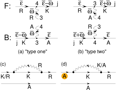
Figure 7: (a) Vertices of “type one” and (b) of “type two” arising in Keldysh perturbation theory; the accompanying Keldysh Green’s functions are $\tilde{G}^{K}(\varepsilon\mp\bar{\omega})$, respectively, producing Pauli factors $\tanh[(\varepsilon\mp\bar{\omega})/2T]$ that dress the associated interaction propagators $\bar{\cal L}{}^{R}$ and $\bar{\cal L}{}^{A}$ [Eq. (107)]. (c,d) Standard Keldysh rules generate diagrams such as both (c) and (d), but the latter vanishes upon impurity averaging, since it contains $G^{A}$ on the forward propagator.

It should be emphasized that the possibility of using such a dressing recipe is a feature peculiar to the Keldysh diagrammatics of disordered systems, as opposed to a generic interacting many-fermion model (see Fig. 7): When inserting interaction lines into the two-particle propagator, standard Keldysh rulesRammerSmith in general also lead to contributions like $G^{K}(\varepsilon-\bar{\omega})\bar{\mathcal{L}}^{K}(\bar{\omega})$, which would spoil the above prescription of not dressing $\bar{\mathcal{L}}^{K}$. However, for disordered systems, such diagrams vanish to leading order, since instead of containing the usual retarded/advanced electron propagators $G^{R/A}$ on the forward/backward contour [as e.g. in Fig. 7(c)], they contain $G^{A/R}$ there [as e.g. in Fig. 7(c)], and after disorder averaging, $\left\langle G^{R/A}G^{R/A}\right\rangle_{{\rm imp}}\approx 0$.

The decay function $F_{d}^{\textrm{pp}}(t)={1\over\hbar}\langle S_{\textrm{eff}}^{\textrm{pp}}\rangle_{\textrm{rw}}$, can be calculated in complete analogy to Sections IV.2 and IV.3: Averaging as usual over time-reversed pairs of random walks using Eq. (34), and calculating the effective noise correlator $\langle VV\rangle_{{\bar{q}}\bar{\omega}}^{\textrm{eff}}$ occuring therein using Eqs. (35) and Eqs. (LABEL:subeq:LAA'FT), we now find that the dressed $\tilde{\cal L}^{R/A}$ factors do not drop out (in contrast to what happens in Eq. (58) when calculating $\langle VV\rangle_{{\bar{q}}\bar{\omega}}^{\textrm{sqn}}$ with undressed propagators). Instead, the effective noise correlator is now given by $\langle VV\rangle_{{\bar{q}}\bar{\omega}}^{\textrm{eff}}\mapsto\langle VV\rangle_{{\bar{q}}\bar{\omega}}^{\textrm{pp}}$ of Eq. (76), and the decay function (34) takes the form of $F_{d}^{\textrm{pp}}(t)$ of Eq. (75). Thus, by using dressed propagators we recover precisely the Pauli-blocked correlator $\langle VV\rangle_{{\bar{q}}\bar{\omega}}^{\textrm{pp}}$ that we had conjectured on heuristic grounds in Section V.4.

Further justification for using the latter noise correlator will be offered by the Bethe-Salpeter analysis of paper II, which leads to a decay function involving precisely the same Pauli-blocked noise correlator [cf. Eqs. (II.LABEL:eq:exponentBetheSalpeter)]. To be somewhat more precise: the Bethe-Salpeter analysis of paper II improves upon the analysis of paper I by keeping track of the energy difference $\omega$ (neglected in paper I, see Ref. wneq0, ) between the energies $\varepsilon$ and $\varepsilon-\omega$ of the particle and hole trajectories, which is why the effective interaction propagator $\bar{\cal L}{}^{\textrm{dec}}_{{\cal E}\omega,{\bar{\bm{q}}}}({\bar{\omega}})$ of Eq. (II.LABEL:eq:define:Ldeco) depends on $\omega$. The latter propagator can actually be obtained from Eq. (35) for $\langle VV\rangle_{{\bar{q}}\bar{\omega}}^{\textrm{eff}}$ by the methods of the present section, namely by setting $\varepsilon\to(\varepsilon-\omega)$ in the Pauli-factors associated with the backward contour when calculating the dressed the correlators $\langle V_{a}V_{a^{\prime}}\rangle^{\textrm{pp}}_{{\bar{q}}\bar{\omega}}$, i.e. in Eqs. (107b) and (107d), with corresponding changes in Eqs. (LABEL:subeq:LAA'FT). However, once the $\omega$-dependence is retained, the expression for $F_{d}(t)$ needs another Fourier integral $\int d\omega e^{-i\omega t}$, i.e. Eqs. (34) or (75), and our intuitive determination of the factor $\delta{\bar{P}}$ therein, become inadequate. A more complete expression for $F_{d}(t)$, including this additional integral, is given by Eq. (II.LABEL:eq:C1tauexplicit). However, in the long-time limit $\max\{T,\varepsilon\}t\gg 1$ of present interest, for which $\omega/\max\{T,\varepsilon\}\ll 1$, Eq. (II.LABEL:eq:C1tauexplicit) reduces to Eq. (II.LABEL:eq:exponentBetheSalpeter), which reproduces our Eq. (75).

Finally, having been alerted to the necessity of keeping track of energy transfers, we note that the vertex diagrams transfer energy between the forward and backward contours, thereby changing the energy of both. Strictly speaking, it is thus not fully correct to assign definite, fixed, energies $\varepsilon$ and $\varepsilon-\omega$ to the upper and lower contours, since a succession of vertex insertions will produce an accumulation of frequency transfers. This effect is neglected in the influence functional approach. This is admissable, essentially because the dominant contribution of vertex insertions comes from the infrared regime ${\bar{\omega}}\sim 1/t$, so that the ${\bar{\omega}}$-dependence in the remaining parts of the diagram may be dropped (they only generate terms subleading in time). This point is discussed in more detail at the end of Sec. LABEL:sec:2ndorderexpansion of Paper II (and also in Sec. B.6.2 of LABEL:vonDelft04).

VII.2 Importance of recoil

To conclude this section, let us point out that the effective action $S_{\textrm{eff}}^{\textrm{GZ}}$ derived by GZ is essentially the same as our $S_{\textrm{eff}}^{\textrm{pp}}$ [Eq. (108)]; the only difference is that in their approach, the dressed correlators emerge in the position-time representation of Eq. (56) [as opposed to the ${\bar{q}}\bar{\omega}$ representation of our Eqs. (LABEL:subeq:LAA'FT)], in which each $\tilde{\cal L}^{R/A}_{ij}$ is dressed by a Pauli factor $[1-2\tilde{\rho}]_{\bar{i}i}$, or $[1-2\tilde{\rho}]_{j\bar{j}}$, where $\tilde{\rho}_{ij}=\langle\psi^{\dagger}_{j}(t)\psi_{i}(t)\rangle$ is the single-particle density matrix. They wrote their effective action as $S^{\textrm{GZ}}_{\textrm{eff}}=iS_{R}+S_{I}$, in which $S_{R}$ contains Pauli factors and $S_{I}$ does not. When averaging over time-reversed pairs of trajectories, GZ used unrestricted random walks, $F^{\textrm{GZ}}_{d}(t)={1\over\hbar}\langle S_{\textrm{eff}}^{\textrm{GZ}}\rangle_{\textrm{urw}}$. Moreover, they employed a position-momentum representation in which they represented the Pauli factors as $\bigl{[}1-2f\bigl{(}\varepsilon(t)\bigr{)}\bigr{]}$.

Up to this point, their approach is essentially equivalent to ours. Differences arise at their next step: in order to perform the average over paths, GZ assumed the energy of the diffusing electron to remain constant along its path GZexplicitcite , arguing that its collisions with the static impurities are elastic, and hence replaced $f\bigl{(}\varepsilon(t)\bigr{)}$ by $f(\varepsilon)$. As shown by von Delft vonDelft04 , this assumption is equivalent to making the replacement $\varepsilon\pm{\bar{\omega}}\to\varepsilon$ in the dressed propagators of our Eqs. (LABEL:subeq:LAA'FT), although this is by no means obvious in GZ’s formalism. In other words, they (unwittingly) neglected the $\pm{\bar{\omega}}$ in the Fermi functions occuring in the Pauli factors, and thereby neglected the recoil experienced by the diffusing electron upon interacting with its environment and emitting or absorbing a noise quantum. [The fact that GZ neglect recoil was first pointed out by Erikson and Hedegard EH97 .] As a result, GZ’s terms affected by Pauli blocking all cancel each other, mistakenly causing $\langle iS^{R}\rangle_{\textrm{urw}}$ to vanish, so that the resulting decay function $F^{\textrm{GZ}}_{d}(t)={1\over\hbar}\langle S_{I}\rangle_{\textrm{urw}}$ is identical to one for a single particle (no Pauli blocking) under the influence of quantum noise. Indeed $F^{\textrm{GZ}}_{d}(t)$ can GZresultVertex be brought into the form of our $F^{\textrm{sqn}}_{d,\textrm{urw}}(t)$ [Eq. (57)]. As discussed in Section IV.4, the resulting decoherence rate is the same as would be found for the physical situation of a single, highly excited electron moving through a disordered sample very high above the Fermi surface, or in the absence of a Fermi sea, and interacting with a quantum environment. Such an electron can lose its coherence even at zero temperature by spontaneous emission, uninhibited by Pauli blocking, which is why GZ obtained a nonvanishing decoherence rate at $T=0$. Indeed, using $\bar{\omega}_{\rm u}=1/{\tau_{\textrm{el}}}$ as upper cutoff in Eq. (66) for the decoherence rate of a single particle experiencing quantum Nyquist noise at $T=0$, we recover precisely GZ’s zero-temperature decoherence rate for all three values of $d$, including numerical prefactors: $\gamma_{\varphi,d}^{\textrm{sqn}(T=0)}=\gamma^{\textrm{GZ}(T=0)}_{\varphi,d}$ [i.e. our Eq. (66) reproduces the $T=0$ values of GZ’s Eqs. (77) and (81) of Ref. GZ2, ].

VIII Conclusion

In this paper, we have shown why it is essential to incorporate the Pauli principle in a description of decoherence by a quantum-mechanical environment, and how this can be achieved in an influence functional description of weak localization. We have explicitly demonstrated how Pauli blocking counteracts the effects of spontaneous emission to ensure that the decoherence rate vanishes for sufficiently small temperatures and energies.

At the beginning of this paper, we offered a review of the influence functional approach for a single electron in a classical environment, pointing out along the way that quantitative improvements can be achieved by performing trajectory averages with respect to closed (as opposed to unrestricted) random walks.Montambaux04 . We then explained how to extend the influence functional methodology to the case of a quantum environment, taking due account of the Pauli principle.

In our approach, a fully quantum-mechanical environment may be treated in complete analogy to the much simpler case of classical noise. To this end, the quantum noise spectrum is modified in a well-defined way that involves Fermi functions, in order to take the place of the classical noise spectrum in the calculation of the Cooperon decay function (and the resulting decoherence time). We have shown how this replacement can be motivated heuristically using a transparent physical picture for the decay of a superposition of two many-body states, which shows that the basic idea of the present approach is general enough to be extended to situations different from weak localization. In limits where the Pauli principle is ineffective, our theory reduces to the Feynman-Vernon influence functional, with a nonvanishing decoherence rate even at zero temperature. In contrast, for electrons propagating near the Fermi surface Pauli blocking is very important: it serves to essentially suppress the decohering effects of quantum fluctuations, confirming the results of Altshuler, Aaronov and Khmelnitskii, which were derived by keeping only the classical (thermal) part of the fluctuations. Moreover, our approach has also enabled us to calculate quantitatively the leading corrections to the decoherence rate, and to discuss in detail the energy-dependence of the decoherence rate (and the Cooperon decay function), also for energies higher than the temperature.

Paper II will be devoted to substantiating these results with the full machinery of Keldysh diagrammatic perturbation theory.

Appendix A Evaluation of ${{\cal P}}(z)$

In this appendix we derive Eqs. (43) for $F_{d}(t)$ and (44) for ${{\cal P}}_{d}(t)$, starting from Eqs. (40).

The latter contains the function $\delta{\tilde{P}}_{d}(\tau_{34},{\widetilde{\tau}}_{34})$, defined in Eq. (42)), which may be calculated as follows: We render the momentum integral in Eq. (42) Gaussian using the integral representation

$${e^{-{\bar{q}}^{2}Dt\tau}\over{\bar{q}}^{2}D}={e^{-{\bar{q}}^{2}Dt}\over{\bar{q}}^{2}D}-t\tau\int_{1/\tau}^{1}dx\,e^{-{\bar{q}}^{2}Dt\tau x}\;,$$ (110)

then perform the Gaussian $\int(d{\bar{q}})$ integral, and finally the auxiliary $\int dx$ integrals, obtaining (with $L_{t}=\sqrt{Dt}$):

$$\delta{\tilde{P}}_{d}(\tau,{\widetilde{\tau}}) = {2^{2-d}\over\pi^{d/2}g_{d}(L_{t})}\left\{\begin{array}[]{l}\sqrt{{\widetilde{\tau}}}-\sqrt{\tau}\rule[-5.69054pt]{0.0pt}{0.0pt}\\ {\textstyle\frac{1}{2}}\ln({\widetilde{\tau}}/\tau)\rule[-5.69054pt]{0.0pt}{0.0pt}\\ {1\over\sqrt{\tau}}-{1\over\sqrt{{\widetilde{\tau}}}}\end{array}\right\}\;\textrm{for}\;\left\{\begin{array}[]{l}d=1\rule[-5.69054pt]{0.0pt}{0.0pt}\\ d=2\rule[-5.69054pt]{0.0pt}{0.0pt}\\ d=3\end{array}\right\}\!.$$ (117)

Inserting these expressions into Eq. (40) and performing the $d\tilde{t}_{34}$ integral results in Eq. (43) for the decay function $F_{d}(t)$, where for closed random walks we obtain

$${{\cal P}}_{1}^{\textrm{crw}}(z) = {{1\over\pi^{1/2}}}\left[(2z\!-\!3)\bigl{[}(1\!-\!z)z\bigr{]}^{1\over 2}+{\textstyle{1\over 2}}\cos^{-1}{(2z\!-\!1)}\right],\rule[-5.69054pt]{0.0pt}{0.0pt}$$

$${{\cal P}}_{2}^{\textrm{crw}}(z) = {{1\over\pi}}\Bigl{[}2(z-1)-\ln z\Bigr{]},$$ (119a)

$${{\cal P}}_{3}^{\textrm{crw}}(z) = {{1\over\pi^{3/2}}}\left[\bigl{[}(1\!-\!z)/z\bigr{]}^{1\over 2}-\cos^{-1}{(2z\!-\!1)}\right],$$

(with $$\cos^{-1}(2z-1)\in[\pi,0] z\in[0,1]$$ for ), whereas for unrestricted random walks we get

$${{\cal P}}_{1}^{\textrm{urw}}(z) = {{1\over\pi^{1/2}}}\left[{\textstyle{8\over 3}}(1\!-\!z)^{3\over 2}-4(1\!-\!z)z^{1\over 2}\right]\;,$$

$${{\cal P}}_{2}^{\textrm{urw}}(z) = {{1\over\pi}}\left[(1-z)\Bigl{(}\ln\bigl{[}(1-z)/z\bigr{]}-1\Bigr{)}\right],\qquad\phantom{.}$$ (119b)

$${{\cal P}}_{3}^{\textrm{urw}}(z) = {{1\over\pi^{3/2}}}\left[(1\!-\!z)/z^{1\over 2}-2(1-z)^{1\over 2}\right].$$

Expanding ${{\cal P}}_{d}(z)$ for small values of its argument yields Eqs. (44) of the main text.

Appendix B Frequency representation for $F_{d,\textrm{urw}}(t)$

In this appendix we discuss the derivation of Eq. (45), which expresses $F_{d,\textrm{urw}}(t)$ in terms of a frequency integral. We shall begin, however, more generally, by considering the case of closed random walks, starting from Eq. (34) for $F_{d,\textrm{crw}}(t)$, with $\langle VV\rangle^{\textrm{eff}}_{{\bar{q}}\bar{\omega}}$ given by Eq. (39). Setting $t_{4}\to-t_{4}$ in the vertex term of Eq. (36a) for $\delta{\bar{P}}^{\textrm{crw}}$ yields the combination $[e^{-i\bar{\omega}t_{34}}-e^{-i\bar{\omega}\widetilde{t}_{34}}]{\bar{P}}^{\textrm{crw}}_{(0,t)}({\bar{q}},t_{34})$. Expressing the latter factor through the first line of Eqs. (33), we obtain

$$F_{d,\textrm{crw}}(t) = \int{(dq)(d\bar{q})(d\bar{\omega})}\,{{\mathcal{W}}_{\textrm{eff}}(\bar{\omega})\over\hbar\nu D{\bar{q}}^{2}}{K_{q{\bar{q}}\bar{\omega}}^{t}\over{\tilde{C}}^{0}(0,t)}\;,\qquad\phantom{.}$$ (120)

where we have defined the kernel [with $\Delta=(E_{q-{\bar{q}}}-E_{q})$]

$$K_{q{\bar{q}}\bar{\omega}}^{t} = 2\!\int_{-{t\over 2}}^{{t\over 2}}\!\!dt_{3}\int_{-{t\over 2}}^{t_{3}}\!\!dt_{4}\left[e^{-i\bar{\omega}t_{34}}-e^{-i\bar{\omega}\widetilde{t}_{34}}\right]e^{-E_{q}t-\Delta t_{34}}$$

$$= 2e^{-E_{q}t}\left[{\Delta t\over\Delta^{2}+\bar{\omega}^{2}}\left(1-{\sin(\bar{\omega}t)\over\bar{\omega}t}\right)\right.$$

$$\qquad\quad\left.+\;{e^{-t(\Delta+i\bar{\omega})}-1\over(\Delta+i\bar{\omega})^{2}}\;-\;{e^{-t\Delta}-e^{i\bar{\omega}t}\over\Delta^{2}+\bar{\omega}^{2}}\right].$$

The corresponding expressions for $F_{d}^{\textrm{urw}}(t)$ have the same form, but [in accord with Eqs. (4)] without the $\int(dq)$ integral and the factor $1/{\tilde{C}}^{0}$, and with $E_{q}=0$ in the integrand, so that $\Delta\mapsto\Delta_{0}\equiv D{\bar{q}}^{2}$, $K_{q{\bar{q}}\bar{\omega}}^{t}/{\tilde{C}}^{0}\mapsto K_{0{\bar{q}}\bar{\omega}}^{t}$.

To proceed further, the spectrum ${\mathcal{W}}_{\textrm{eff}}(\bar{\omega})$ has to be specified. For the case of classical white Nyquist noise, where it is given by ${\mathcal{W}}_{\textrm{cl}}(\bar{\omega})=T$, the frequency integrals can be performed explicitly by contour methods, yielding

$$F^{\textrm{cl}}_{d,\textrm{crw}}(t) = Tt\int{(dq)(d{\bar{q}})\over{\tilde{C}}^{0}(0,t)}{e^{-E_{q}t}\over\hbar\nu D{\bar{q}}^{2}}\left\{1-\frac{1-e^{-\Delta t}}{\Delta t}\right\},$$

(122)

$$F^{\textrm{cl}}_{d,\textrm{urw}}(t) = Tt\int(d\bar{q})\,\frac{1}{\hbar\nu D{\bar{q}}^{2}}\left\{1-\frac{1-e^{-\Delta_{0}t}}{\Delta_{0}\,t}\right\}.$$

For $F^{\textrm{cl}}_{d,\textrm{urw}}(t)$, this result stems purely from the first line of Eq. (B), since the two terms in its second line each (separately) give zero. [Note that Eqs. (122) are actually obtained most easily by performing the $\int(d\bar{\omega})$ integral in Eq. (120) before the time integrals.] Both expressions for $F^{\textrm{cl}}_{d}(t)$ are free of infrared divergences as ${\bar{q}}\to 0$ [in accord with the discussion after Eq. (42)], but for $d=2,3$, they are ultraviolet divergent, as discussed at the end of Sec. VI.1. For $d=1$, the momentum integrals can be performed by first rendering them Gaussian, using the integral representation $(1-e^{-b})/b=\int_{0}^{1}dx\,e^{-bx},$ and performing the auxiliary $dx$ integrals last, whereupon Eqs. (50) are recovered.

For non-trivial choices of ${\mathcal{W}}_{\textrm{eff}}(\bar{\omega})$, such as ${\mathcal{W}}_{\textrm{sqn}}$ or ${\mathcal{W}}_{\textrm{pp}}$ for quantum noise, the $\int(d\bar{\omega})$ integral has to be performed last. To make progress with the momentum integrals, let us make some simplifications (which the main text manages to avoid): Firstly, we shall henceforth study only the case of unrestricted random walks, $F_{d,\textrm{urw}}(t)$ [whose asymptotic large-$t$ behavior differs from that of $F_{d,\textrm{crw}}(t)$ only for $d=1$, as shown in the main text]. Secondly, we shall retain only the term in the first line of Eq. (B) for $K_{0{\bar{q}}\bar{\omega}}^{t}$, which dominates the behavior for large $t$, and drop the “subleading” terms in the second line (which yield zero for ${\mathcal{W}}_{\textrm{cl}}$, as mentioned above). Performing the $\int(d{\bar{q}})$ integral in Eq. (120) using

$${2\over\pi}\int{(d{\bar{q}})\over\hbar\nu D{\bar{q}}^{2}}\left[{\Delta_{0}\over\Delta_{0}^{2}+\bar{\omega}^{2}}\right]=p_{d}\,\bar{\omega}^{d/2-2}\;,$$ (123)

we obtain Eq. (45) of the main text, with $p_{1}=\sqrt{2\gamma_{1}}/\pi$, $p_{2}=1/(g_{2}2\pi)$, $p_{3}=1/(\sqrt{2\gamma_{3}}\,\pi^{2})$ [for $\gamma_{1},g_{2},\gamma_{3}$, see Eq. (11)].

References

- (1) E. Abrahams, P. W. Anderson, D. C. Licciardello, and T. V. Ramakrishnan, Phys. Rev. Lett. 42, 673 (1979).
- (2) B. L. Altshuler, D. E. Khmelnitskii, A. I. Larkin, and P. A. Lee, Phys. Rev. B 22, 5142 (1980).
- (3) B. L. Altshuler, A. G. Aronov, D. E. Khmelnitskii, A. I. Larkin, “Quantum Theory of Solids”, edited by I. M. Lifshitz (Mir Publishers, Moscow) 1982.
- (4) G. Bergmann, Phys. Rep. 107, 1 (1984).
- (5) P. A. Lee and T. V. Ramakrishnan, Rev. Mod. Phys. 57, 287 (1985).
- (6) S. Chakravarty and A. Schmid, Phys. Rep. 140, 193 (1983).
- (7) B. Kramer and A. MacKinnon, Rep. Prog. Phys. 56, 1469 (1993).
- (8) D. S. Golubev and A. D. Zaikin, Phys. Rev. Lett. 91, 1074 (1998).
- (9) D. S. Golubev and A. D. Zaikin, Phys. Rev. B 59, 9195 (1999).
- (10) D. S. Golubev and A. D. Zaikin, Phys. Rev. B 62, 114061 (2000).
- (11) D. S. Golubev, A. D. Zaikin, and G. Schön, J. Low Temp. Phys. 126, 1355 (2002) [cond-mat/0110495].
- (12) D. S. Golubev and A. D. Zaikin, Journal of Low Temperature Physics, 132, 11 (2003) [cond-mat/0208140].
- (13) D. S. Golubev, C. P. Herrero, and A. D. Zaikin, cond-mat/0205549.
- (14) D. S. Golubev, G. Schön, A. D. Zaikin, J. Phys. Soc. Jpn. 72, Suppl. A (2003) [cond-mat/0208548].
- (15) I. Aleiner, B. L. Altshuler, and M. E. Gershenzon, Waves in Random Media 9, 201 (1999) [cond-mat/9808053]; Phys. Rev. Lett. 82, 3190 (1999).
- (16) K. A. Eriksen and P. Hedegard, cond-mat/9810297; GZ replied in cond-mat/9810368.
- (17) M. Vavilov and V. Ambegaokar, cond-mat/9902127.
- (18) T. R. Kirkpatrick and D. Belitz, cond-mat/0112063, cond-mat/0111398.
- (19) I. L. Aleiner, B. L. Altshuler, and M. G. Vavilov, J. Low Temp. Phys. 126, 1377 (2002) [cond-mat/0110545].
- (20) Y. Imry, cond-mat/0202044.
- (21) F. Marquardt, cond-mat/0207692.
- (22) I. L. Aleiner, B. L. Altshuler, and M. G. Vavilov, cond-mat/0208264.
- (23) J. v. Delft, J. Phys. Soc. Jpn. Vol. 72 (2003) Suppl. A pp. 24-29 [cond-mat/0210644].
- (24) J. v. Delft, ”Influence functional for Decoherence of Interacting Electrons in Disordered Conductors”, in ”Fundamental Problems of Mesoscopic Physics”, I. V. Lerner et al. (eds), p. 115-138 (2004) [cond-mat/0510563].
- (25) B. L. Altshuler, A. G. Aronov, and D. E. Khmelnitskii, J. Phys. C 15, 7367 (1982).
- (26) J. von Delft, F. Marquardt, R.A. Smith, V. Ambegaokar, cond-mat/0510557.
- (27) The benefit of restricting the average to self-returning random walks has been independently recognized by G. Montambaux and E. Akkermans, private communication, and cond-mat/040404361, version 2. See also Ref. AkkermansMontambaux04, .
- (28) A. Voelker and P. Kopietz, Phys. Rev. B 61, 13508-13514 (2000).
- (29) H. Fukuyama and E. Abrahams, Phys. Rev. B 27, 5976 (1983).
- (30) P. Mohanty, E. M. Q. Jariwala, and R. A. Webb, Phys. Rev. Lett. 78, 3366 (1997); Fortschr. Phys. 46, 779 (1998).
- (31) In the condition which we use to define , our choice of 1 as threshold constant is somewhat arbitrary, leading to a corresponding arbitrariness in the numerical prefactor of the resulting ; this arbitrariness does not, however, affect the function itself, or the magnetoconductivity derived therefrom.
- (32) A. Stern, Y. Aharonov, and Y. Imry, Phys. Rev. A 41,3436 (1990); see also Y. Imry, “Introduction to Mesoscopic Physics”, Second Edition, Oxford University Press (2002).
- (33) Ref. AAK, of AAK is known to contain various incorrect factors of two. They can be eliminated by replacing in AAK’s Eq. (6), and rederiving all subsequent equations. For example, one needs in Eq. (9) and in Eqs. (19) and subsequent equations, e.g. (20), (22), (23), (26) and (28), so that their decoherence time () and magnetoconductivity () take the forms given in this paper (or by Eqs. (2.38b) and (2.42c) of Ref. AAG, , respectively).
- (34) In this paper, temperature is measured in units of frequency, i.e. stands for throughout; likewise, although will often be referred to as “excitation energy”, it stands for a frequency.
- (35) R. P. Feynman and F. L. Vernon, Ann. Phys. (NY) 24, 118 (1963); R. P. Feynman and A. R. Hibbs, “Quantum Mechanics and Path Integrals”, McGraw-Hill (1965);
- (36) Actually, we shall calculate the Cooperon for finite times, , i.e. we need for nonzero frequencies. Thus, the energies of the particle and hole trajectories should strictly speaking differ by , i.e. we should talk these energies to be and , respectively. However, it will turn out that in order to determine , we need to know only in the long-time limit where , implying , so that the energy difference between particle and hole trajectories can be neglected. We shall do so throughout paper I, but in paper II include the -dependence, and confirm by explicit calculation (Paper II, App. LABEL:app:checkF1) that it produces corrections that are negligble for .
- (37) The leading term of Eq. (16a) has also been derived in Ref. vonDelft04, .
- (38) F. Pierre, A. B. Gougam, A. Anthore, H. Pothier, D. Esteve, and Norman O. Birge, Phys. Rev. B 68, 085413 (2003).
- (39) Two examples of noise with a Gaussian distribution are classical white Nyquist noise, or the Coulomb interaction, treated in the random phase approximation.
- (40) See the discussion after Eq. (9.14) of Ref. CS ; the sign in front of is wrong.
- (41) F. Marquardt, cond-mat/0410333.
- (42) B. L. Altshuler and A. G. Aronov, Solid State Commun. 38, 1031 (1981).
- (43) In AAG’s Eq. (4.13b), the factor contains a typo: it should be (private correspondence with I. Aleiner).
- (44) The result corresponds to AAG’s Eq. (4.9b) after correcting for two typos in LABEL:AAG: their Eq. (4.3b) needs an extra factor of on the right-hand side, implying that the in their Eq. (4.9b) should be replaced by .
- (45) H. Pothier, S. Gu ron, Norman O. Birge, D. Esteve, and M. H. Devoret, Phys. Rev. Lett. 79, 3490 (1997).
- (46) J. Rammer and H. Smith, Rev. Mod. Phys. 58, 323 (1986).
- (47) This assumption is stated in Ref. GZ2 , in the first sentence after Eq. (68): the Fermi function “depends only on the energy and not on time because the energy is conserved along the classical path.”
- (48) By averaging GZ’s decay function , defined in Eq. (22) of Ref. GZ3, , over time-reversed pairs of unrestricted random walks using Eq. (29), it can be brought into the form of our [Eq. (57)]. Moreover, setting in our Eq. (45), with replaced by of Eq. (58b), we immediately recover GZ’s defining relation for , as given in Eq. (76) of Ref. GZ2, (except that they inserted the infrared cutoff by hand and determined it selfconsistently, because in Ref. GZ2, they did not evaluate the vertex contributions explicitly; the latter were included fully in Ref. GZ3, ).
- (49) E. Akkermans and G. Montambaux, “Physique msoscopique des lectrons et des photons”, EDP Sciences 2004, http://www.lps.u-psud.fr/Utilisateurs/gilles/livre.htm