Propagation and Backscattering of Mechanical Impulses in a Gravitationally Loaded Chain: Dynamical Studies and Toy Model Based Phenomenology

Abstract

We recently introduced a simple toy model to describe energy propagation and backscattering in complex layered media (T.R. Krishna Mohan and S. Sen, Phys. Rev. E 67, 060301(R) (2003)). The model provides good qualitative description of energy propagation and backscattering in real soils. Here we present a dynamical study of energy propagation and backscattering in a gravitationally loaded granular chain and compare our results with those obtained using the toy model. The propagation is ballistic for low $g$ values and acquires characteristics of acoustic propagation as $g$ is increased. We focus on the dynamics of the surface grain and examine the backscattered energy at the surface. As we shall see, excellent agreement between the two models is achieved when we consider the simultaneous presence of acoustic and nonlinear behavior in the toy model. Our study serves as a first step towards using the toy model to describe impulse propagation in gravitationally loaded soils.

I Introduction

Acoustic imaging of buried objects in a non-linear medium like nominally dry soil is still an open problem senburied . Amongst its main applications, we can mention the problem of locating antipersonnel land mines, human remains for forensic investigations, hidden underground structures of archaeological importance etc. It has been shown that gentle mechanical impulses rogdon can be used to detect buried objects at depths of a meter or so in nominally dry sand beds. Imaging requires the understanding of pulse propagation in nonlinear media. Besides the underlying non-linearity due to the Hertzian contact forces between the grains (see, for example, Landau 1970 ), gravitational loading is an added feature that affects the dynamics. Before we can analyze the gravitational effects in 3D systems, it is reasonable first to look at the problem in 1D. Further motivation for 1D studies can be found in mosen .

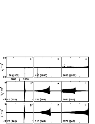
Figure 1: In Fig. 1(a)-(c), $g=0$ and we see solitary wave propagation. In Fig. 1(d)-(f), $g=0.1$ and in Fig. 1(g)-(i), $g=1.0$. In both cases, open boundary conditions are employed at the top with closed boundary conditions at the bottom. We see solitary wave like front with a long tail for non-zero $g$. The text in the lower left hand corner indicates the times at which the snapshots are taken and, in brackets, is given the roundtrip time, i.e. the time taken by the pulse to travel up and down the chain once. The $y$-axis ranges have been marked in the leftmost panel for each row of panels while the $x$-axis range is the same in all and labelled in the top left panel, Fig. 1(a), where $j$ is the position of the particle in the chain and $V_{j}$ its velocity.

Impulse propagation in a gravitationally loaded chain with $N$ grains and a perfectly reflecting boundary at the bottom has been studied Sinkovits 1995 ; Sen 1996 ; nest . When $g=0$, one finds solitary wave propagation Ne83 ; Sinkovits 1995 as shown via velocity vs. position plots made at different times in Figs. 1(a)-(c) (see later for simulation details). In all the panels of Fig. 1, the numbers in the bottom left corner indicate the times at which the snapshots have been taken and, in brackets, the round trip time of the pulse is given.

The velocity of the solitary wave is a function of its amplitude Ne83 ; Sinkovits 1995 ; Manciu 1999 III ; SenManciu pre 2001 . Each solitary wave is reflected at the bottom boundary. During reflection, the solitary wave forms secondary solitary waves Manciu pre 2001 ; JobSen ; quasi . Further, secondary solitary waves are generated from collisions with other solitary waves mosen . The formation of secondary solitary waves progressively reduces the amplitude of the solitary waves in the system. In Fig. 1(c), we find that the amplitude of the primary solitary wave has diminished considerably after $2.6$ roundtrips.

When $g>0$, one finds a solitary wave like front with a tail that elongates with time Hong 2001 ; Hong 1999 ; Manciu 2000 . In Figs. 1(d)-(f), we have shown snapshots from the propagation of the impulse in a system with $g=0.1$ and with open boundary condition at the top. We have the same boundary conditions in Figs. 1(g)-(i) with $g=1.0$. We see that the impulse propagates faster with increased $g$.

The scheme of this paper is as follows. Section II surveys briefly the $1$-$D$ model with the simulation details. Our focus is to probe impulse propagation and backscattering by simply considering the dynamics of the surface grain. In Section III, we construct a version of the toy model and recover the results obtained in section II. Section IV summarizes the conclusions for the $1$D study and assesses the usefulness of this study for further $3$D analysis.

II Simulation model

We model the granular chain as a collection of $10000$ spherical grains which are placed in contact with one another and loaded by a gravitational field. The interaction between every pair of spheres of radius $R$ is driven by Hertz law Landau 1970 ; Sinkovits 1995 , i.e., it is assumed that spheres labeled as $i$ and $i+1$ are interacting with a potential proportional to the overlaps, $\delta_{i,i+1}$, in the contact region,

$$V(\delta_{i,i+1})=\begin{cases}a\ \delta_{i,i+1}^{5/2}&\text{if $r_{i,i+1}\leq 2R$}\\ 0&\text{if $r_{i,i+1}>2R$}\end{cases}$$ (1)

where $a$ is a constant that depends upon the material characteristics of the grains, $r_{i,i+1}$ is the separation distance between the centers of the grains $i$ and $i+1$ and $\delta_{i,i+1}\equiv 2R-r_{i,i+1}$ is the grain overlap. The equation of motion for grain $i$ can be written as Manciu 2000 ,

$$m\overset{\cdot\cdot}{z_{i}}=\frac{5}{2}a\left(\delta_{i,i-1}^{3/2}-\delta_{i+1,i}^{3/2}\right)-mg\text{,}$$ (2)

where $m$ and $g$ are the mass of the grain and the value of gravity, respectively. The system dynamics is obtained by time integration of the coupled Newtonian equations of motion via the velocity-Verlet algorithm Tildesley 1987 . We ignore the role of dissipation in the present study; dissipation effects can be built in later diss . We set $2R$ and $m$ to $1$, and $a$ is set equal to $5657$. We find that an integration time step of $1\times 10^{-5}$ provides excellent enrgy conservation; decreasing the time step further does not improve the accuracy of our results. Particles are labeled starting from the bottom so that the $N$${}^{\mbox{\small th}}$ particle is at the top. While the bottom boundary condition has been kept perfectly reflecting in all the simulations, both open and closed boundary conditions have been employed at the top in different simulations to investigate the differences induced by the particular choice.

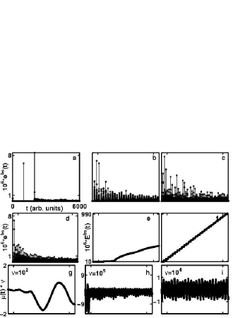
Figure 2: In Fig. 2(a), $g=0$, in Fig. 2(b) $g=0.1$, and in Figs. 2(c)-(d), $g=1.0$. Figs. 2(a)-(c) have closed boundary conditions at the top while Fig. 2(d) has open boundary condition at the top. Typical integrated backscattered energy, $E^{bs}(t)$, plots are shown in Figs. 2(e)-(f) where Fig. 2(e) is for $g=0.0$ and Fig. 2(f) for $g=0.1$ with top closed boundary condition (cf. Fig. 2(b)). The center of mass, $\mu$, oscillations typically found in these systems are given in the third row of panels. Fig. 2(g) is for $g=0.0$ while Fig. 2(h) is for the top closed boundary condition ($g=0.1$; cf. Fig. 2(b) and Fig. 2(f)). Fig. 2(i) is for the top open boundary condition (cf. Fig. 2(d)). The $x$-axis remains the same in all panels as labelled in Fig. 2(a) with the time, $t$, given in arbitrary units (a.u.) of the simulation. $y$-axis ranges for the first row is given in the leftmost panel, and separately labelled for each panel in the bottom row. For the middle row, the first panel on the left has a different $y$-axis range as shown and, for the last two panels, it is as shown for the middle panel.

The dynamics is initiated via an initial velocity perturbation at the top of the chain, $v_{N}(t=0)=v_{in}$, with $v_{i}(t=0)=0$ for $0\leq i<N$; we have employed $v_{in}=-0.01$ in the studies reported here. We subsequently monitor the backscattered energy received at the surface, $e^{bs}(t)=v_{N}^{2}(t)/2$. The time integrated backscattered energy, $E^{bs}(t)$, has also been computed by summing the entire sequence of energy packets received at the surface, i.e. $E^{bs}(t)=\sum_{t^{\prime}=0}^{t}e^{bs}(t^{\prime})$.

In Fig. 2(a-d), we show plots of $e^{bs}(t)$ vs. $t$. Fig. 2(a) is obtained with $g=0.0$. We have two prominent peaks at early times followed by a continuous distribution of much smaller peaks. Clearly, the smaller peaks originate in the breakdown of the solitary waves at the boundaries and through mutual interactions (this issue is discussed in detail in quasi ). The two large peaks at early times are separated by roundtrip times of the system. Fig. 2(b) corresponds to $g=0.1$, with reflecting boundary conditions at the top in which the surface grain is only allowed to move in one direction into the chain. In this case, there are large peaks separated by roundtrip times of the system, but there is much activity in between them indicating the presence of acoustic like rattling throughout the system. Increasing $g$ to $1.0$ (Fig. 2(c)), with the same boundary conditions, does not reveal any noticeable change in the pattern except for increasing the density of peaks, caused by the smaller roundtrip times. If we keep $g=1.0$ and change to open boundary conditions, meaning that the surface grain is allowed to move up and down, we get the pattern shown in Fig. 2(d) where we notice that the number of larger peaks are reduced. We attribute this to increased energy sharing caused by the open boundary at the top.

The $E^{bs}(t)$ vs. $t$ plots show a distinct difference between the ballistic and acoustic type propagation cases. While Fig. 2(e) is for the $g=0$ case, Fig. 2(f) is typical of $g>0$ cases (here, $g=0.1$ with closed boundary at the top). The increase is linear for non-zero $g$ whereas it only approaches linear for $g=0.0$ in the later stages. The steps in $E^{bs}(t)$ indicate the arrival of peaks with the quiescent period in between marked by plateaus; the length of the plateau indicates the time period between peaks.

The pattern of arrival of large peaks introduce modulations in the amplitudes of $e^{bs}(t)$. Nevertheless, there are no simple patterns in the distribution of peaks of $e^{bs}(t)$ vs. $t$ in Figs. 2(a-d). We note that the boundary conditions affect $e^{bs}(t)$. A possible modulating mechanism could be due to the center of mass (com) oscillations of the system. We show these oscillations (the “breathing” of the chain) in the third row of Fig. 2 for three typical cases. With $g=0$ (Fig. 2(g)), the significant com oscillations appear only after the solitary waves have broken down. For non-zero $g$, the com oscillations are affected by the surface boundary. Fig. 2(h) is for $g=0.1$ and with closed boundary conditions at the top while Fig. 2(i) is typical of open boundary conditions at the top (in this case, $g=1.0$). We now turn to the toy model to see whether these patterns in $e^{bs}(t)$ can be reproduced.

III Comparison with toy model

We had introduced a toy model in an earlier paper where the energy propagation in a vertical alignment of masses was considered in a simplified manner mosen . At time $t=0$, we set initial energy $E=1$ for layer one and zero for the rest. At $t=1$, the first layer in the vertical chain transfers $p$ ($<1$) of the impulse energy to the second layer, and retains $(1-p)$. At subsequent times, the impulse will propagate in the same fashion all the way down the chain. After each transfer of energy, the phase of the mass reverses so that it will interact with its adjacent layer in the opposite direction in the following time step. The interaction between two adjacent layers occurs in the following two ways: (i) equipartition case, and (ii) exchange case. In the equipartition case, the two interacting layers will come away from the interaction with equal amounts of energy; we add up the individual energies of the two layers and divide the sum equally between them. In the exchange case, we let the layers exchange their energies; the two interacting layers, after the interaction, come away with the energy of the other.

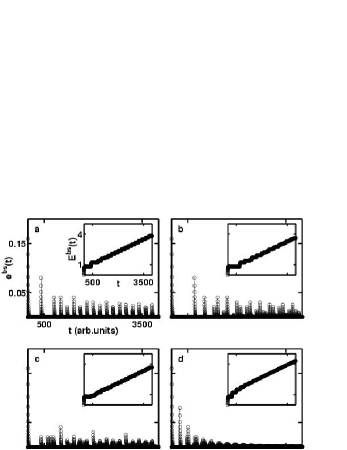
Figure 3: All the panels along with the insets have the axes ranges as labelled in the top left panel. Fig. 3(a) is for the case of a single equipartition center in the toy model located at particle no. 200 out of a total of 500 particles in the chain, and Fig. 3(b) for the case, similarly, with equipartition center at particle no. 350; the exchange coefficient $p=0.8$. Data for these two cases have been averaged, along with data for cases with single equipartition centers located at 300 and 390 respectively, and presented in Fig. 3(c). In Fig. 3(d), we have multiple equipartition centers located at particle nos. 125, 230 and 390 with $p=0.8$.

In Fig. 3, we show the results where the model has, for the first time, both equipartition and exchange. Our goal is to develop the propagation patterns seen in Figs. 2(b-d). The model is based on the exchange case, but we allow equipartition centers to develop, as time goes by, at different points in the chain. In Fig. 3(a), we have shown a case where a single equipartition center is kept fixed at layer number 200 in a chain of 500 layers. Fig. 3(b) is for a similar case but with the equipartition center located at layer number 350. We see that the patterns in $e^{bs}(t)$ do change slightly depending on the location of the isolated equipartition center, but, in both cases, it is seen that the patterns are broadly similar to the non-zero $g$ cases seen in Figs. 2(b)-(d).

This has prompted us to try averaging over the patterns resulting from differing locations of the isolated equipartition centers and, indeed, the plot of Fig. 3(c) shows that such averaging does retain the similarity with plots of Figs. 2(b)-(d). To obtain this figure, we averaged over, along with the cases given in Fig. 3(a) and Fig. 3(b), two other cases with isolated equipartition centers, in each case, located at layer numbers 300 and 390 respectively. If we vary the exchange coefficient $p$, we get similar patterns (not shown here) but with the difference that the growth in $E^{bs}(t)$ is proportional to the $p$ value. This indicates that $p$ could also be used, along with the equipartition centers, to capture the transition from ballistic propagation to acoustic propagation. In Fig. 3(d), we show results with multiple (three, in this cases) equipartition centers in the system, at layer numbers 125, 230 and 390; $p=0.8$ for this case. We see that $E^{bs}(t)$ grows by as much as in Figs. 3(a)-(c) but the attenuation in peaks of $e^{bs}(t)$ is very pronounced and similar to the pattern seen in Fig. 2(d).

IV Summary and conclusions

In this paper, we have studied the problem of impulse propagation in a gravitationally loaded granular chain. We have focused our attention on the backscattered energy received at the surface after an impulse has been initiated into the system. Our studies have been carried out using two different approaches— (i) using Newtonian dynamics in a non-disspative system to describe backscattering at the surface of the system and, (ii) using the toy model mosen to recover the behavior in (i).

Our results show that the toy model is capable of reproducing the correct form of the backscattered energy as a function of time in a gravitationally loaded chain. Gravitational loading introduces acoustic-like oscillations in the system. Such oscillations vanish and the system ends up propagating solitary waves when gravitational loading is zero. To achieve these descriptions, one must generalize the earlier version of the toy model mosen and incorporate both exchange (represents non-linear) and equipartition (represents acoustic) effects. We find that the role of the equipartition (acoustic) effect in the toy model is rather dominant and only limited equipartitioning of energy gives the correct backscattering behavior. Our studies confirm that mechanical propagation in a granular chain is strongly nonlinear even in the presence of gravitational loading.

V Acknowledgment

EA acknowledges the Fulbright Foundation for support. TRKM and SS have been supported by the Army Research Office and NASA.

References

- (1) G. Baker, C. Schmeissner, D. W. Steeples and R. G. Plumb, Geophys. Res. Lett. 26, 279 (1999); S. Hostler, Ph.D. Thesis, Mechanical Engineering, California Institute of Technology (2005); S. R. Hostler and C. E. Brennen, Phys. Rev. E 72, 031303 (2005); ibid. 72, 031304 (2005); D. P. Visco, Jr., S. Swaminathan, T. R. Krishna Mohan, A. Sokolow and S. Sen, Phys. Rev. E 70, 051306 (2004). S. Sen, T. R. Krishna Mohan, D. Visco, Jr., S. Swaminathan, A. Sokolow, E. Avalos and M. Nakagawa, Int. J. Mod. Phys. 19, 2951 (2005).
- (2) A. Rogers and C. G. Don, Acoust. Austral. 22, 5 (1994); M. J. Naughton et al. IEE Conf. Proc. 458, 249 (1998); S. Sen et al., ibid. 4394, 607 (2001).
- (3) H. Hertz, J. reine u. Angew. Math. 92, 156 (1881); L. D. Landau and E. M. Lifshitz, Theory of Elasticity, 2nd Ed., Pergamon Oxford, 1970.
- (4) T. R. Krishna Mohan and S. Sen, Phys. Rev. E 67, 060301(R) (2003).
- (5) R. S. Sinkovits and S. Sen, Phys. Rev. Lett. 74, 2686 (1995).
- (6) S. Sen and R. S. Sinkovits, Phys. Rev. E 54, 6857 (1996).
- (7) V. Nesterenko, Dynamics of Heterogeneous Materials, Springer-Verlag, Berlin, 2001.
- (8) V. Nesterenko, J. Appl. Mech. Tech. Phys. 5, 733 (1983); A. Lazaridi and V. Nesterenko, ibid. 26, 405 (1985); C. Coste, E. Falcon and S. Fauve, Phys. Rev. E 56, 6104 (1997); A. Chatterjee, Phys. Rev. E 59, 5912 (1999).
- (9) S. Sen and M. Manciu, Phys. Rev. E 64, 056605 (2001).
- (10) S. Sen and M. Manciu, Physica A 268, 644 (1999).
- (11) M. Manciu, S. Sen and A. J. Hurd, Phys. Rev. E 63, 016614 (2001).
- (12) S. Job, F. Melo, A. Sokolow and S. Sen, Phys. Rev. Lett. 94, 178002 (2005).
- (13) S. Sen, J. M. M. Pfannes and T. R. Krishna Mohan, J. Kor. Phys. Soc. 46, 571 (2005); T. R. Krishna Mohan and S. Sen, Pramana— J. of Physics 64, 423 (2005).
- (14) J. Hong and A. Xu, Phys. Rev. E 63, 061310 (2001).
- (15) J. Hong and J. Y. Ji, H. Kim, Phys. Rev. Lett. 82, 3058 (1999).
- (16) M. Manciu, V. Tehan and S. Sen, Chaos 10, 658 (2000).
- (17) M. P. Allen and D. J. Tildesley, Computer Simulation of Liquids, Clarendon, Oxford, 1987.
- (18) O. R. Walton and R. L. Braun, J. Rheol. 30, 949 (1986); N. V. Brilliantov, F. Spahn, J. M. Hertzsch and T. Pöschel, Phys. Rev. E 53, 5382 (1996); S. Sen, M. Manciu and A. J. Hurd, Physica D 157, 226 (2001).