Néel and disordered phases of coupled Heisenberg chains with $S=\frac{1}{2}$ to $S=4$

Abstract

We use the two-step density-matrix renormalization group method to study the effects of frustration in Heisenberg models for $S=\frac{1}{2}$ to $S=4$ in a two-dimensional anisotropic lattice. We find that as in $S=\frac{1}{2}$ studied previously, the system is made of nearly disconnected chains at the maximally frustrated point, $J_{d}/J_{\perp}=0.5$, i.e., the transverse spin-spin correlations decay exponentially. This leads to the following consequences: (i) all half-integer spins systems are gapless, behaving like a sliding Luttinger liquid as in $S=\frac{1}{2}$; (ii) for integer spins, there is an intermediate disordered phase with a spin gap, with the width of the disordered state is roughly proportional to the 1D Haldane gap.

I Introduction

An important theorem by Dyson, Lieb, and Simon (DLS) states that the Heisenberg Hamiltonian on bipartite lattices with $S\geq 1$ have long-range order in the ground state dls ; neves . We now know from quantum Monte Carlo simulations young that this result extends to $S=\frac{1}{2}$ systems. There is current interest as to how a disordered state emerges out of the Néel state. This question is important to the physics of frustrated materials where some systems exhibit no magnetic order down to the experimentally accessible temperatures and are thus believed to be disordered in the ground state. A disordered phase may also be relevant in the theory of high temperature superconductors. This issue and the related one of the eventual role of Berry phases was hotly debated in the late 1980’s and early 1990’s soon after the discovery of the high $T_{C}$ materials dombre ; stone ; zee ; affleck1 ; haldane2 . Many possible disordered states were proposed but none of them gained consensus. For an extensive discussion on this topic, we refer the reader to the book by Fradkin fradkin .

In the search of the nature of a ground state of a quantum Hamiltonian, there is another useful theorem by Lieb, Schultz, and Mattis (LSM)lsm , initially formulated for 1D systems and later extended to 2D systems by Affleck affleck1 restricts the possible ground states of half-integer spin systems. Either the ground state is degenerate, (presumably due to a broken symmetry) or it is unique and gapless without any long-range order. For Heisenberg Hamiltonians, the latter possibility appears difficult to realize in 2D because dimer-dimer or spin-spin correlations have a power law decay in 1D. It would thus be expected that interchain couplings will lead to long-range order in one of the two channels. If the magnetic order is frustrated, a dimerization would be expected. Frustrated spin models often involve competitions between two magnetic orders, the expected dimerized phase is believed to lie between these magnetic phases. A possible alternative to this scenario allowed by the LSM theorem is the occurence of a disordered gapless state at transition between the magnetic phases.

In recent publications moukouri-TSDMRG ; moukouri-TSDMRG2 , we have studied the possible emergence of a disordered state in a model of coupled Heisenberg chains. This model is a spatially anisotropic version of the well studied $J_{1}-J_{2}$ model. The model essentially retains the physics of the $J_{1}-J_{2}$ model: it presents a phase transition between two magnetic phases. The first phase is a Néel phase characterized by the ordering wave vector $Q=(\pi,\pi)$. The order parameter in this phase is maximal in absence of the diagonal coupling $J_{d}$. It decreases as $J_{d}$ is increased until it vanishes at the maximally frustrated point. Beyond this point, another Néel state with $Q=(\pi,0)$ becomes the ground state. The existence of these two phases was predicted in numerous studies lhuillier of the isotropic ($J_{\perp}=1$) version of this model. But what has caused the continuing interest into this simple model is the question of whether there is an intermediate phase between these two magnetic phases. Simple physical arguments suggest the existence of such a phase because the two states are associated with subgroups of the $SU(2)$ symmetry group of the spin Hamiltonian and of the $C_{4}$ symmetry group of the square lattice that neither include each other. From the Landau theory we know that a continuous transition from these two phases is forbidden. Initial suggestions for the possible intermediate phase was the resonating valence bond (RVB) baskaran phase, flux phases marston ; kotliar , chiral spin liquid wen or the spin-Peierls (SP) read . The SP phase has lately emerged as the front runner. It causes the same type of difficulty as the direct transition between two magnetic phases. Since in that case, the transition is between a magnetic state that breaks the spin rotational symmetry but not the lattice translational symmetry to a dimerized state that breaks the lattice translational symmetry but not the spin rotational symmetry. The transition to SP phase has triggered interesting proposal of an extension of the conventional Landau-Ginzburg-Wilson (LGW) theory of second order phase transitiondc .

It seems, however, that this theory does not apply to the $J_{1}-J_{2}$ model, where we did not find any evidence of an intermediate phase for $S=\frac{1}{2}$. Numerical data suggests a transition, which seems to be of second order, between the two magnetic phases at the maximally frustrated point for both the anisotropic and isotropic models moukouri-TSDMRG3 . At the transition point, the competing magnetic orders neutralize each other and the system behaves like a collection of loosely bound chains, even if the bare interactions are not small. Classically, the ground state is degenerate at this point. This degeneracy is lifted by quantum fluctuations. In Ref.moukouri-TSDMRG2 ; moukouri-TSDMRG3 , we have shown that among all the possible clusters, chains offer the best compromise between minimizing the energy and avoiding frustration at the same time. At the maximally frustrated point, the transverse interactions seem to be irrelevant. I.e., up to the largest lattice size studied, transverse spin-spin correlations decay exponentially and the longitudinal correlations revert to those of decoupled chains. This disordered state is a singlet and gapless consistent with the LSM theoremlsm ; affleck1 . It is reminiscent of a sliding Luttinger liquid (SLL) found in models of coupled fermions chains carpentier ; kivelson ; kane . It thus appears that the intermediate region where a disordered phase has long been thought to exist is just a critical region. That is the reason why it has resisted various approaches for nearly two decades. At the maximally frustated point, the correlation functions are 1D-like, thus the rotational spin symmetry of the system is restored. In fact such a transition between these two magnetic phases already exists in the unfrustred model when the transverse exchange parameter, $J_{\perp}$, is varied from positive values to negative values. At the point $J_{\perp}=0$, there is a transition from 2D to 1D, where properties are identical to that of the maximally frustrated point. The only difference between the case $J_{\perp}=0$ and the maximally frustrated point is the presence of irrelevant transverse terms which do not change the long distance behavior of the correlation functions as shown in Ref.moukouri-TSDMRG2 . From this result the LGW theory applies if it is assumed that the system’s group of symmetry at the critical point contains the groups of symmetry of the two magnetic phases.

It is important to study how this interesting physics extends to larger spin systems. First, because many frustrated systems contain larger spins. Second, because there are some interesting predictions from large $S$ approaches about the emergence of a disordered phase from a Néel phase as function of $S$. Affleck affleck1 argued that since the LSM theorem does not apply to integer spin systems, there might be a distinction between integer and half-integer spin systems in 2D as well. Haldane haldane2 discussed that in addition to the now well-established distinct behavior between half-integer and integer spins in one dimension haldane1 , there might be a difference between odd and even integer spins in two dimensions due to the effects of the Berry phase. Read and Sachdev carried out a large $N$ analysis of the possible disordered phase as function of the value of the large $N$ equivalent of the spin. Their results were consistent with Haldane’s predictions. Three types of disordered states were predicted. For half-integer spins, the non-magnetic phase is a SP phase which breaks the translational symmetry along the two directions of the square lattice. For odd integer spins, the non-magnetic state is made of weakly-coupled chains, i.e., the translational symmetry is broken along one direction only. Finally for even integer spins, the disordered state are valence bond solids, like the Affleck-Kennedy-Lieb-Tasaki (AKLT) stateaklt , i.e, it does not break any translational symmetry.

In the large $S$ approaches the Heisenberg model is mapped onto the non-linear sigma model ($NL\sigma$) with a Berry phase term. This mapping is only approximatehaldane1 ; affleck and there can be some subtle differences with the original modelaffleck . Indeed, the realization of the Haldane conjecture in 1D shows their power. But, in absence of exact results for small $S$, it is impossible to know whether their predictions of a disordered phase extends to small $S$. Another potential problem is that the mapping to the $\sigma$-model assumes the presence of a smooth configuration of spins. This is true in the weak-coupling regime (Néel ordered phase). But this assumption may break down in the strong coupling regime (disordered phase). In one dimension, the $\sigma$-model coupling constant is given by $g=2/(\sqrt{S(S+1)}\sqrt{1-4J_{2}})$ affleck . Thus for $S=\frac{1}{2}$, the equivalence between the two models breaks down at $J_{2}=0.25$, i.e., close to the transition to a dimerized state. Such a breakdown seems to occur in the $J_{1}-J_{2}$ model where, as seen above, the large $N$ predictions conflict for $S=\frac{1}{2}$ with the TSDMRG in the $J_{1}-J_{2}$ model. But since spin-half integer systems are critical, it could be objected that the behavior seen in our numerical studies are due to finite size effects. For large enough lattices there might be a relevant interaction which can drive the system to a SP phase as predicted from large $N$. Though this scenario appears to be unlikely, as discussed in Ref.moukouri-TSDMRG3 , it cannot be completely rejected. In principle, one would expect a different behavior for integer spin systems which are known to have a spin gap in 1D haldane1 .

In this paper, we applied the TSDMRG to study $S=\frac{1}{2}$, $1$, $\frac{3}{2}$,…,$4$ systems in the anisotropic 2D Hamiltonian (1). Our results in the absence of frustration are in agreement with the DLS theorem Ref.dls ; neves . We find that for all $S$ the ground state is ordered in the absence of frustration. For all $S$ except for $S=\frac{1}{2}$, the order parameter is large enough so that the extrapolated value are reliable. This result constitutes a non-trivial test of the TSDMRG, since the TSDMRG starts from decoupled chains which are disordered. When the frustration is turned on, the general mechanism found for the destruction of the Néel phase is the severing of the frustrated bonds in the transverse direction, leading to a disordered state with the transverse correlations that decay exponentially at the critical point as previously found for $S=\frac{1}{2}$. However, a different conclusion is to be drawn for half-integer $S$ and for integer $S$ for which the LSM theorem does not apply. All half-integer systems are similar to $S=\frac{1}{2}$. The disordered state is confined at the critical point, it has a SLL character. But for integer $S$, because of the Haldane gap $\Delta_{H}$ in the chain, there is an intermediate phase whose width is roughly $\propto\Delta_{H}$.

This paper is organized as follows. In the next section we discuss the model and the method. In section (III), we present extensive results for $S=1$ systems. This analysis is similar to the one made for spin $\frac{1}{2}$ systems in Ref.moukouri-TSDMRG3 . In section (IV) the results for systems with $S=\frac{1}{2}$ to $4$ are presented. In section (V), we present our conclusions.

II Model and Method

II.1 model

We apply the TSDMRG moukouri-TSDMRG ; moukouri-TSDMRG2 to the spatially anisotropic Heisenberg Hamiltonian,

$$H=J_{\parallel}\sum_{i,l}{\bf S}_{i,l}{\bf S}_{i+1,l}+J_{\perp}\sum_{i,l}{\bf S}_{i,l}{\bf S}_{i,l+1}$$

$$+J_{d}\sum_{i,l}({\bf S}_{i,l}{\bf S}_{i+1,l+1}+{\bf S}_{i+1,l}{\bf S}_{i,l+1})$$ (1)

where $J_{\parallel}$ is the intra-chain exchange parameter and is set to 1; $J_{\perp}$ and $J_{d}$ are respectively the transverse and diagonal interchain exchanges. This model is the object of current interest tsvelik ; moukouri-TSDMRG2 ; sindzingre ; starykh . It is a starting point of understanding the $J_{1}-J_{2}$ model which is recovered when $J_{\parallel}=J_{\perp}=J_{1}$ and $J_{d}=J_{2}$. It retains the basic physics of the $J_{1}-J_{2}$ model and has the advantage that in the limit $J_{\perp},J_{d}\ll 1$, well tested 1D results can be used to initialize a perturbative RG analysis.

II.2 The two-step DMRG

In the TSDMRG, to study a 2D lattice of size $L\times(L+1)$ ( we will refer to the 2D systems only by their linear dimension $L$), we start by applying the usual 1D DMRG ($m_{1}$ states are kept) or exact diagonalization (ED) to a single chain $l$ of length $L$ to obtain $m_{2}$ low lying eigenstates and eigenvalues, $\phi_{n_{l}}$, $\epsilon_{n_{l}}$, $n_{l}=1,2,...m_{2}$, respectively. Then, we formally write the tensor product of the $L+1$ chains,

$$\Phi_{[n]}=\phi_{n_{1}}\phi_{n_{2}}...\phi_{n_{L+1}}.$$ (2)

$\Phi_{[n]}$ is an eigenstate of the Hamiltonian with $J_{\perp}=0.$ and $J_{d}=0$, $[n]=(n_{1},n_{2},...,n_{L+1})$. The $\Phi_{[n]}$ constitute a many-body basis of the truncated Hilbert space of the tensor product of $L+1$ chains. The corresponding eigenvalue is:

$$E_{[n]}=\epsilon_{n_{1}}+\epsilon_{n_{2}}+...+\epsilon_{n_{L+1}}$$ (3)

The 2D Hamiltonian (1) is then projected onto this truncated basis to yield an effective one dimensional Hamiltonian which is studied using the DMRG.

The TSDMRG is perturbative; but the expansion is made onto the smaller term of the Hamiltonian itself not on the Green’s function or the ground-state wave function. We have shown that starting from a disordered state, the TSDMRG is able to reach the ordered state without any addition of a term that explicitly breaks the symmetry such as a magnetic field. The TSDMRG was tested against the quantum Monte Carlo (QMC) method in Ref.(moukouri-TSDMRG2 ) and against ED in Ref.(alvarez ). The TSDMRG is variational, its performance can systematically be improved by increasing $m_{1}$ and $m_{2}$. Key indicators about the performance of the TSDMRG are the truncation error $\rho_{1}$ during the first step, the width $\delta E$ of the $m_{2}$ states kept and the truncation error $\rho_{2}$ during the second step. In principle, it is necessary that the ratio of $\delta E$ over the transverse coupling be large for the TSDMRG to yield great accuracy. Typically, one must have $\delta E/J_{\perp}\approx 10$. If this condition is fulfilled and the $m_{2}$ states are accurate enough, .ie., $\rho_{1}$ is small, the TSDMRG method can reach the QMC accuracy. So far, this has been achieved only for small couplings $J_{\perp}\lesssim 0.1$ and lattice sizes of up to $L=16$ keeping up to $m_{2}=96$. The amount of calculations involved remains modest and so far are done on a workstation. The accuracy decreases by increasing $J_{\perp}$ leading to less accurate results in the ordered state. But when both $J_{\perp}$ and $J_{d}$ are turned on, the performance of the TSDMRG becomes more complex as we will see below.

In this work, the calculations for $S=1$ were performed similarly to those for spin $S=\frac{1}{2}$ systems in Ref.moukouri-TSDMRG3 . In most cases, ED was applied during the first step. In some case, i.e, some runs of $L=10$ and all runs of $L=12$, a single DMRG iteration was used. For instance for $L=10$ and $S=1$, when $m_{1}=81$ states are kept, a single $DMRG$ iteration is necessary to reach desired size. For this calculation, we kept up to $m_{2}=96$ states during the second TSDMRG step. For the maximum performance of the algorithm, it is necessary that $J_{\perp}$ be in the order of the finite size gap of the single chain $\Delta_{L}$. For $S=1$, $\Delta_{L}\rightarrow\Delta_{H}$ when $L\rightarrow\infty$, where $\Delta_{H}=0.4107$ white is the Haldane gap. A second condition to fulfill is $\delta_{L}\gg J_{\perp}$ where $\delta_{L}$ is the width of the retained eigenvalues. As noticed in Ref.moukouri-TSDMRG3 , the TSDMRG is more accurate in the highly frustrated regime. In Fig.(1) we show the truncation error, $\rho_{2}$, when two states are targeted in the second step as function of $J_{d}$ for $S=1$ and $J_{\perp}=0.4$. $\rho_{2}$ is minimal near $J_{d}=0.22$. At this point the system is an assembly of nearly disconnected chains; the DMRG is thus expected to perform better.

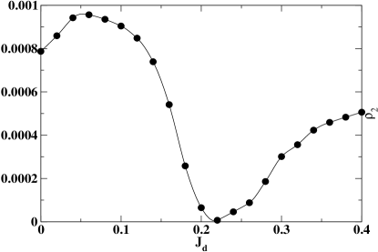
Figure 1: Truncation error in the second TSDMRG step as function of $J_{d}$ for $J_{\perp}=0.4$, $S=1$ and $L=10$, ED was performed in the first step and in the second step, $m_{2}=64$.

II.3 Illustration in the $S=1$ case

We now wish to provide a detailed description of a typical TSDMRG calculation. For this illustration, $S=1$ and $L=12$, i.e, following the convention set above, the size of the 2D lattice is $12\times 13$. We start the usual 1D DMRG iteration keeping $m_{1}=243$ states, i.e, the initial superblock size is $L=12$. At this point the DMRG is equivalent to ED. At the next iteration, the superblock size is $L=14$, its total number of states is $M_{s}=(3\times 243)^{2}$. The size of the reduced superblock (the superblock minus the two single site blocks) size is $L=12$. During this iteration, spins sectors with $S_{T}^{z}=0,\pm 1,\pm 2,\pm 3$ are targeted. The lowest states in each of these sectors for $L=12$ have respectively the following energies, $E_{0}=-16.8696$, $E_{\pm 1}=-16.3854$, $E_{\pm 3}=-16.2780$. The truncation error is $7.3\times 10^{-7}$. The reduced superblock is then diagonalized and the $m_{2}=64$ lowest lying states are kept. The energy of the highest state among these $m_{2}$ states is $-14.2687$ which is lower than $E_{\pm 4}=-12.6524$, the lowest states of the $S_{T}^{z}=\pm 4$ sectors. For this reason, these sectors was not targeted. The operators ${\bf S}_{i}$ at each site are stored and updated.

From the energy levels above, we see that the finite size spin gap is $\Delta_{L}=0.4842$, which is not very far from its value $\Delta_{H}=0.4107$ in the thermodynamic limit. Our choice of $J_{\perp}=0.4$ ensures that the chains will effectively be coupled at this size. The matrix $O$ whose columns are made of the $m_{2}$ vectors $\phi_{n}$ kept is used to express all the operators in the truncated reduced superblock basis,

$${\bf{\bar{S}}}_{i}=O^{\dagger}{\bf S}_{i}\delta_{3,3^{\prime}}O,$$ (4)

the intra-chain Hamiltonian is likelywise updated

$$h=O^{\dagger}(h_{B_{1}}\delta_{3,3^{\prime}}+h_{B_{3}}\delta_{1,1^{\prime}})O.$$ (5)

In these equations, we have adopted the usual convention that the different blocks of the superblock are labelled $1-2-3-4$. For PBC, blocks $2$ and $4$ are made of a single site and blocks $1$ and $3$ are the largest blocks. In Eq. (4), it is supposed that the spin to update is in block $1$. In Eq. (5), $h_{B_{i}}$ represents the internal Hamiltonian of block $i$. The first step ends with the updating of these operators.

Each chain may now be viewed as a super ’spin’ with additional internal degrees of freedom due to the different sites. A chain $l$ is described by its ’spin’ value ${\tilde{\bf S}}_{l}=({\bf{\bar{S}}}_{il},i=1,...,L)$ and its internal Hamiltonian $h_{l}$. $h_{l}$ is diagonal in the basis of the $m_{2}$ states kept. The effective first order Hamiltonian which approximates the original 2D Hamiltonian is now given by

$$H_{eff}=\sum_{l}h_{l}+J_{\perp}\sum_{l}{\tilde{\bf S}}_{l}*{\tilde{\bf S}}_{l+1}+J_{d}\sum_{l}{\tilde{\bf S}}_{l}\times{\tilde{\bf S}}_{l+1},$$ (6)

where,

$${\tilde{\bf S}}_{l}*{\tilde{\bf S}}_{l+1}=\sum_{i}{\bf{\bar{S}}}_{i,l}{\bf{\bar{S}}}_{i,l+1}$$ (7)

and

$${\tilde{\bf S}}_{l}\times{\tilde{\bf S}}_{l+1}=\sum_{i}{\bf{\bar{S}}}_{i,l}{\bf{\bar{S}}}_{i+1,l+1}+{\bf{\bar{S}}}_{i+1,l}{\bf{\bar{S}}}_{i,l+1}.$$ (8)

We then proceed to compute the low lying states of $H_{eff}$ using the conventional DMRG again. For this simulation we keep $m_{2}$ states and use $3$ blocks instead $4$ to form the superblock.

As expected from the study of $S=\frac{1}{2}$ systems, the TSDMRG is more accurate in the highly frustrated regime than in the unfrustrated case. $\rho_{2}$ is relatively large in the unfrustrated regime because of the relatively large value of the interchain coupling. The same simulation with $J_{\perp}=0.2$ leads to an improvment of factor $10$. It is worth noting that the superblock size in this step is $m_{2}^{3}$, we are able to reach $m_{2}=100$ on a workstation, this remains modest with respect to what can be achieved on today’s supercomputers. For the multi-chain DMRG superblock sizes of about $100$ times larger are accessible jeckelmann , this means that it is possible to reach $m_{2}\approx 500$ on a supercomputer. This would increase the current accuracy of the TSDMRG by two or more orders of magnitude. This shows the great potential of the TSDMRG. These possibilities are under exploration.

III Results for $S=1$

The case of spin $\frac{1}{2}$ has been extensively studied in Ref.moukouri-TSDMRG2 ; moukouri-TSDMRG3 . We were able to reach lattice sizes of up to $64\times 65$ and show that as seen in QMC simulations, the system is ordered in absence of frustration for small $J_{\perp}$. But when $J_{d}\neq 0$, we have shown that in the vicinity of $J_{d}/J_{\perp}\approx 0.5$ the system is made of weakly-coupled chains even when $J_{\perp}$ and $J_{d}$ are not small. This finding of the TSDMRG was checked using ED on small systems alvarez . More careful simulations at the vicinity of the point $J_{d}/J_{\perp}=0.5$ revealed that the first neighbors interchain correlation, i.e. the transverse bond strength is equal to zero at the maximally frustrated point. The non-zero correlations, starting from the second neighbor decay exponentially. These results lead us to conclude that the maximally frustrated point is a quantum critical point (QCP) between the two magnetic states (the second magnetic state is stable when $J_{d}>0.5J_{\perp}$). A possible argument against this conclusion is that at the maximally frustrated point, the system could be instable against higher orders terms such as a ring exchange term starykh . In the case of a two-leg ladder this term seems to lead to a dimerized state. There are however some strong indications that the dimerized state does not exist in this model as discussed in Ref.moukouri-TSDMRG3 . The mechanism to avoid frustration is to divide the system into chains in which the frustrated bonds are severed. We will now study the extension of this mechanism to $S=1$. We perform the same analysis as for $S=\frac{1}{2}$ for $L=6$, $8$, $10$ and $12$. For the first three values of $L$, ED is performed to obtain the $m_{2}$ lowest eigenvalues and the corresponding eigenstates of the chain. For $L=12$ the DMRG was used, we kept $m_{1}=243$ states, i.e, one DMRG iteration was done from the $L=10$ exact result. The truncation error was about $7\times 10^{-7}$. The truncation error is relatively large because we used periodic boundary conditions. These $m_{2}$ low-lying states were then used to generate the 2D lattices, i.e, $6\times 7$, $8\times 9$, $10\times 11$ and $12\times 13$ respectively.

III.1 Ground-state energies

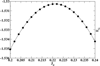
Figure 2: Ground-state energy per site as function of $J_{d}$ for $J_{\perp}=0.4$, $S=1$ and $L=12$.

The curve of $E_{G}(J_{d})$ for $S=1$, shown in Fig.(2) is similar to that of $S=\frac{1}{2}$. Starting from $J_{d}=0$, $E_{G}$ increases until it reaches a maximum at $J_{d}^{max}$. It then decreases when $J_{d}$ is further increased. The position of the maximum depends slightly on $L$ and seems to converge to $0.5J_{\perp}$ in the thermodynamic limit. $E_{G}(J_{d}^{max})$ is very close to $1.53$, the energy of decoupled chains, but always remains slightly lower. Thus as for $S=\frac{1}{2}$ the chains are very weakly bound, even though the bare interactions ($J_{\perp}=0.4$ and $J_{d}=0.22$) are not small. $J_{d}^{max}$ depends on $L$ as shown in Fig.(3) and as in the case of $S=\frac{1}{2}$, it extrapolates to $0.5J_{\perp}$ in the thermodynamic limit.

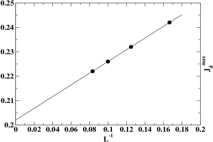
Figure 3: Maxima of the ground-state energy as function of $L$ for $J_{\perp}=0.4$, $S=1$.

$E_{G}(l)$ shown in Fig.(4), where $l$ is the number of chains is dramatically different when $J_{d}$ is far or close to $J_{d}^{max}$. Far from $J_{d}^{max}$, one of the two magnetic phases is highly favored. Starting from an isolated chain, magnetic energy can be gained by increasing $l$, leading to the ordered state. The situation is different when $J_{d}=J_{d}^{max}$; neither of the magnetic states is favored. At this point, magnetic energy cannot be gained and $E_{G}(l)$ is nearly independent of $l$, the system remains disordered as we will see below from the analysis of the correlation functions.

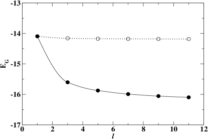
Figure 4: Ground-state energy per chain as function of the chain number for $J_{\perp}=0.4$, $S=1$, $L=10$ for $J_{d}=0$ (filled circles), and $J_{d}=J_{d}^{max}$ (open circles).

III.2 First neighbor correlation

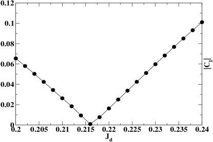
Figure 5: First neighbor spin-spin correlation as function of $J_{d}$ for $J_{\perp}=0.4$, $S=1$, $L=12$.

The transverse first neighbor spin-spin correlation taken in the middle of the lattice

$$C_{1}=\langle S_{L/2,L/2+1}S_{L/2,L/2+2}\rangle,$$ (9)

shown in Fig.(5) is also reminiscent of the $S=\frac{1}{2}$ case. $C_{1}$ vanishes linearly at $J_{d}=J_{d}^{0}$. $J_{d}^{0}$ is slightly different from $J_{d}^{max}$. This small difference is due to numerical error; this conclusion is supported by the more accurate results obtained for small $S=\frac{1}{2}$ systems in Ref.(moukouri-TSDMRG3 ) where $J_{d}^{0}$ and $J_{d}^{max}$ are equal. The extrapolated $J_{d}^{0}$ (Fig.(6) as $L\rightarrow\infty$ is also in the vicinity of $0.5J_{\perp}$.

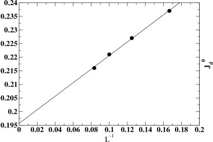
Figure 6: Minima of the first neighbors spin-spin correlation as function of $L$ for $J_{\perp}=0.4$, $S=1$.

III.3 Long-distance correlations

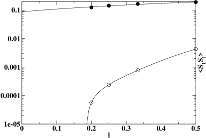
Figure 7: Transverse spin-spin correlation as function of the distance for $L=10$, $S=1$, $J_{\perp}=0.4$, $J_{d}=0$ (filled circles) and $J_{d}=J_{d}^{max}$ (open circles).

The transverse spin-spin correlation function,

$$C_{l}=\langle S_{L/2,L/2+1}S_{L/2,L/2+l}\rangle$$ (10)

is shown in Fig.(7) for a $L=10$ system and $J_{\perp}=0.4$. When $J_{d}=0$, $C_{l}$ extrapolates to a finite value in the thermodynamic limit. This result is important because it shows the non-perturbative nature of the TSDMRG. Starting from an isolated chain which is disordered, the TSDMRG can reach the ordered phase. The ordered phase can be easily reached for larger spin than for $S=\frac{1}{2}$ where quantum fluctuations are more important. The extrapolation of $C_{l}$ for $S=\frac{1}{2}$ leads to a small negative value as shown in Fig.(20) below. In this case, the order parameter is too small to be obtained from an extrapolation from relatively small systems; it is necessary to go to larger systems as those studied in Ref.(moukouri-TSDMRG2 ) in order to extrapolate to the correct thermodynamic limit. The extrapolated value of $C_{l}$ does not however lead to the correct value of the magnetization since it is obtained from a system with a fixed $L$. A better estimation is given by the finite size analysis of the end-to-center spin-spin correlation

$$C_{L}=\langle S_{L/2,L/2+1}S_{L/2,L+1}\rangle$$ (11)

shown in Fig.(8). $C_{L}$ for $L\rightarrow\infty$ is roughly $0.06$ consistent again with the existence of the long-range order.

In the vicinity of $J_{d}^{max}$, $C_{l}$ decays exponentially as seen in Fig.(7). For $l=5$, his value is already four order of magnitude smaller than in the case $J_{d}=0$. This is consistent the nearly disconnected chain behavior observed for $E_{G}$ at this point.

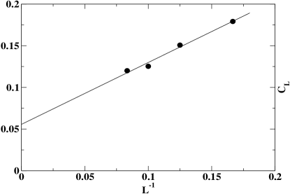
Figure 8: Center-to-end spin-spin correlation as function of $L$ for $S=1$, $J_{\perp}=0.4$ and $J_{d}=0$.

III.4 spin gaps

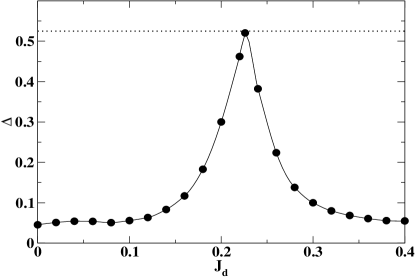
Figure 9: Gap as function of $J_{d}$ for $L=10$, $S=1$; the dotted line represent the single chain gap.

The variation of the spin gap $\Delta$ with $l$ (for a fixed $L$), $L$, and $J_{d}$ the are also consistent with the above findings. $\Delta(J_{d})$ for $L=10$ system is shown in Fig.(9). $\Delta(J_{d}=0)$ is about $0.05$ (in this regime the gap is zero in the thermodynamic limit as we will see below); $\Delta$ remains relatively flat as $J_{d}$ is increased until it reaches the vicinity of $J_{d}^{max}$. Near $J_{d}^{max}$, $\Delta(J_{d})$ first sharply increases and reaches the finite size gap of an isolated chain. As $J_{d}>J_{d}^{max}$, $\Delta(J_{d})$ first sharply decreases and then becomes nearly constant at about $0.05$. $\Delta(l)$ (Fig.(10)) is reminiscent of $E_{G}(l)$; in the unfrustrated case, the chains are effectively coupled. $\Delta(l)$ rapidly decreases from about $0.53$ to $0.05$ as $l$ is varied from $1$ to $11$. At $J_{d}=J_{d}^{max}$ however, $\Delta(l)$ is nearly independent of $l$.

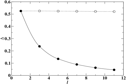
Figure 10: Gap as function of the number of chains for $L=10$, $S=1$, $J_{\perp}=0.4$, $J_{d}=0$ (filled circles) and $J_{d}=J_{d}^{max}$ (open circles).

The analysis $C_{L}$ shows that for $J_{d}=0$, the system is ordered. We thus expect that $\Delta(L)\rightarrow 0$ as $L\rightarrow\infty$. This is seen in Fig.(11) where $\Delta(L)$ is shown for $L=6,8,10$ and $12$ systems. The decay faster than $\frac{1}{L}$, the extrapolation to leads to a negative value. At $J_{d}=J_{d}^{max}$ on the order hand, $\Delta(L)$ remains close to that of an isolated chain in all case. The two functions are finite in the thermodynamic limit. This result show the dramatic difference between $S=\frac{1}{2}$ and $S=1$ systems. For $S=\frac{1}{2}$, an equivalent plot lead to a zero gap moukouri-TSDMRG3 at the maximally frustrated point. The extrapolated value for $J_{d}=0$, $\Delta=0.4015$ agrees well with the current best estimate of the Haldane gap $\Delta_{H}=0.4107$. The difference is due to the relatively short chains, up to $L=16$, that were used for the extrapolation not to the DMRG that yielded highly accurate results for each size studied. Noting that the spin-spin correlations in the transverse direction have a very short range, the difference between the extrapolated values of $J_{d}=0$ and $J_{d}=J_{d}^{max}$ appears to be relatively large. We believe that this difference could be inferred from the fact that the extrapolation from $2D$ systems were done with lattice sizes up to $L=12$ only.

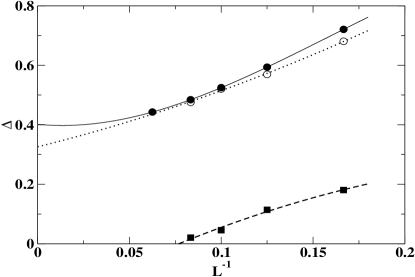
Figure 11: Gap as function of $L$ for $S=1$, $J_{\perp}=0$ and $J_{d}=0$ (single chain, filled circles), $J_{\perp}=0.4$, $J_{d}=0$ (filled squares) and $J_{d}=J_{d}^{max}$ (open circles).

III.5 Spin-spin correlations on large systems

So far, in the study of $S=1$ systems, we have fixed $J_{\perp}=0.4$. This choice was motivated by the presence of $\Delta_{H}=0.4107$ in an isolated chain. We initialy felt that it was necessary to choose a large enough $J_{\perp}$ so that the chains will effectively be coupled when the perturbation is turned on and this will lead to sizable correlation in the thermodynamic limit. But, this choice limited us to relatively small lattices, $L\lesssim 12$. This is because when $J_{\perp}$ is large, the condition $\delta E/J_{\perp}\gg 1$ is hard to fulfill for larger $L$. For instance for $L=16$, $\delta E/J_{\perp}=5.65$ for $m_{2}=64$, this prevented us to study $L=16$ lattices. But in the course of this work, we find that even smaller values of $J_{\perp}$ can lead to detectable values of in the unfrustrated regime $C_{l}$ as $l\rightarrow\infty$. For smaller $J_{\perp}$, we can actually reach larger $L$. We wish to present in this part our results for $J_{\perp}=0.2$ and $L=24$. These results will add strength to those of $J_{\perp}=0.4$ presented above.

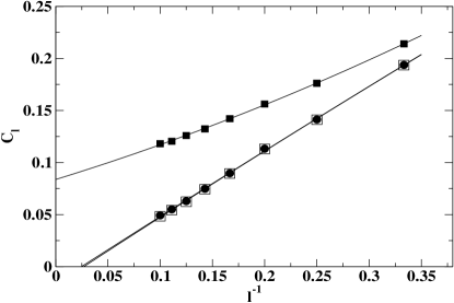
Figure 12: Longitudinal spin-spin correlation as function of the distance for $L=24$, $S=1$, $J_{\perp}=0$, $J_{d}=0$ (filled circles), $J_{\perp}=0.2$, $J_{d}=0$ (filled squares), $J_{d}=0.2$, $J_{d}=0.102$ (open squares).

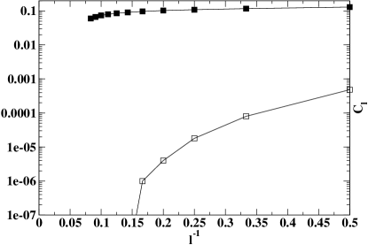
Figure 13: Transverse spin-spin correlation as function of the distance for $L=24$, $S=1$, $J_{\perp}=0$, $J_{d}=0$ (filled circles), $J_{\perp}=0.2$, $J_{d}=0$ (filled squares), $J_{d}=0.2$, $J_{d}=0.102$ (open squares).

In Fig.(12), we show the longitudinal correlation,

$${\bar{C}}_{l}=\langle S_{L/2+1,L/2+1}S_{L/2+l,L/2+1}\rangle,$$ (12)

taken in the middle chain. For $J_{\perp}=0.2$ and $J_{d}=0$, ${\bar{C}}_{l}$ clearly extrapolate to a finite value as expected. But for $J_{\perp}=0.2$ and $J_{d}=0.102$, ${\bar{C}}_{l}$ is nearly identical to spin-spin correlation on an isolated chain. For the transverse correlation $C_{l}$ shown in Fig.(13), we see again the dramatic difference between the unfrustrated and highly frustrated cases. In the first case, $C_{l}$ goes to a finite value when $l\rightarrow\infty$. But for the highly frustrated case $C_{l}$ decays exponentially.

Another picture of this dramatic difference is given by the magnetic structure factor $S(Q=(q_{x},q_{y}))$ shown in Fig.(14,15). In the magnetic phase, $S(Q)$ is dominated by a sharp peak at $Q=(\pi,\pi)$ indicative of Néel order. In the disordered phase, $S(Q)$ is nearly flat except for a small range along $Q=(\pi,q_{y})$ which retains the signature of short-range in chain correlations.

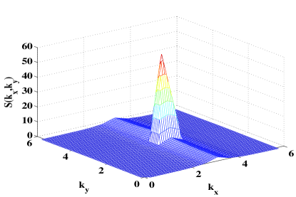
Figure 14: Magnetic structure factor for $L=24$, $S=1$, $J_{\perp}=0.2$, $J_{d}=0$.

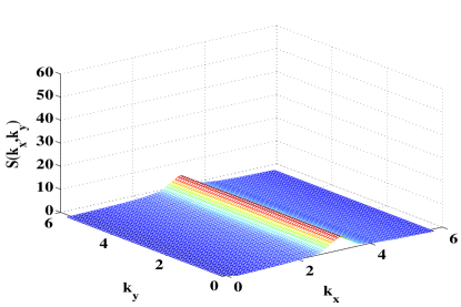
Figure 15: Magnetic structure factor for $L=24$, $S=1$, $J_{\perp}=0.2$, $J_{d}=0.102$.

III.6 Conclusion

In this section, we have presented comprehensive results on $S=1$ coupled chains. These results show some analogy with those of $S=\frac{1}{2}$ published in Ref.(moukouri-TSDMRG3 ). Starting from the unfrustrated system for which $J_{d}=0$, the ground state for $S=1$ is ordered, as expected from the DLS theorem. While for $S=\frac{1}{2}$ it was necessary to simulate lattices of up to $L=64$ moukouri-TSDMRG2 in order to see the extrapolation of $C_{l}$ to a finite value, for $S=1$, relatively short sizes ($L=12$) were enough. This is indeed because quantum fluctuations are less important in a $S=1$ system, i.e., the order parameter is larger. This enables it to be computed more easier. By comparison, the same extrapolation done for $S=\frac{1}{2}$ will lead to a negative value.

When the frustration $J_{d}$ is turned on and reaches the value $J_{d}^{max}$, a point where $E_{G}$ is maximum, $C_{l}$ decays exponentially, $\Delta$ takes a value very close to that of a pure 1D system. These results imply that at $J_{d}^{max}$, the transverse interactions are irrelevant. For $S=\frac{1}{2}$, we identified this state as spin version of an SLL. In that case, this sliding phase will probably be confined at the critical point where the two competing magnetic states $Q=(\pi,\pi)$ and $Q=(\pi,0)$ neutralizes each other. However, we cannot completely rule out a small finite extension of the sliding phase or even totally exclude the emergence of a relevant interaction at lower energies which eventually drives the system to a dimerized phase starykh . It is obvious that, though both $S=\frac{1}{2}$ and $S=1$ systems are made of nearly disconnected chains at $J_{d}^{max}$, the conclusions must be different because of the presence of the Haldane gap $\Delta_{H}$ in the $S=1$ chain. The existence of $\Delta_{H}$ restricts the possible phases that may arise in the vicinity of $J_{d}^{max}$. The first crucial difference is that the disordered state that exist in an $S=1$ system has a gap in its excitation spectrum as seen in Fig.(11); any eventual residual interaction will be wiped out by this gap which means the emergence of new phases at low energies is not favorable for an $S=1$ system. This disordered phase has probably a finite extension which is roughly $\propto\Delta_{H}$.

IV Results for $S=\frac{1}{2}$ to $S=4$

In the study of various $S$, we will not do the same extensive calculation seen in the preceeding section with $S=1$. We will simply fix $L$ and analyze the behavior of the system as function of $J_{d}$ and $l$. As we will see below, quantum fluctuations are small for $S>1$, the study of relatively small systems is enough to get the correct picture in the thermodynamic limit. We studied a lattice with $L\times(L+1)=10\times 11$ for $S=\frac{1}{2}$ to $S=4$. $J_{\perp}$ was set to $0.4$ so that it is larger than the finite size gap in spin half-integer systems and larger or close to the Haldane gaps in spin integer systems. $J_{d}$ is varied from $0$ to $0.4$.

IV.1 Ground-state energies

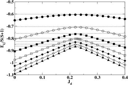
Figure 16: Ground state energy as function of $J_{d}$ and $S=\frac{1}{2}$ (filled circles), $S=1$ (open circles), $S=\frac{3}{2}$ (filled squares), $S=2$ (open squares), $S=\frac{5}{2}$ (filled diamonds), $S=3$ (open diamonds), $S=\frac{7}{2}$, (filled triangles).

The ground-state energy is shown in Fig.(16) for $S=\frac{1}{2}$ to $\frac{7}{2}$. Simulations were also done for $S=4$ but they did not converge for certain values of $J_{d}$. We infer this failure to the large degeneracy of the renormalized single chain Hamiltonian $h_{l}$ for large $S$. At $J_{d}=0$, the curves approach the classical value $E_{G}/S^{2}=-1.4$ quite rapidly. For $S=\frac{7}{2}$, we find $E_{G}/S(S=1)=-1.093$. But if we use the $1/S^{2}$ normalization, we get $E_{G}/S^{2}=-1.405$. Hence if both finite size effects and the correct normalization are taken into account, $S=\frac{7}{2}$ is already in the classical limit.

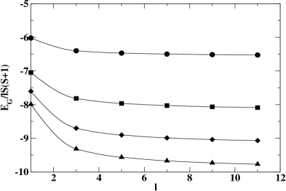
Figure 17: Ground state energy at $J_{d}=0$ as function of $l$ and $S=\frac{1}{2}$ (circles), $S=1$ (squares), $S=\frac{3}{2}$ (diamonds), $S=2$ (triangles)

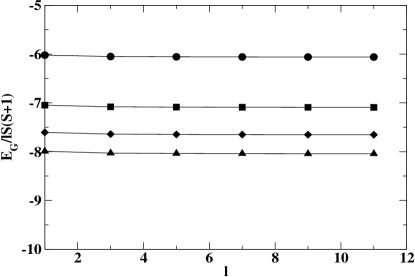
Figure 18: Ground state energy at $J_{d}=0$ as function of $l$ and $S=\frac{1}{2}$ (circles), $S=1$ (squares), $S=\frac{3}{2}$ (diamonds), $S=2$ (triangles)

Larger spin systems are found to present the same features displayed by spin $1/2$ systems. The ground-state energy, $E_{G}$, shown in Fig.(16) increases as $J_{d}$ increases until the maximally frustrated point where $E_{G}$ of the two-dimensional system becomes very close to that of disconnected chains. From this point it decreases when $J_{d}$ is further increased. This may be interpreted as follows: starting from the Néel state with $Q=(\pi,\pi)$ for $J_{d}=0$, the system tends to lose energy under the action of $J_{d}$ which progressively destroys the Néel order until the maximally frustrated point. Beyond this point, $J_{d}$ becomes dominant and the systems enters the Néel $Q=(\pi,0)$ phase. The position of this maximum decreases slowly with increasing $S$. This indicates that in addition to the effect of OBC that shifts $J_{d}^{max}$ towards higher values, there are intrinsic finite size effects. All systems evolve regularly towards the $S\rightarrow\infty$ limit.

The curve of $E_{G}$ appears to change structure as $S$ increases. At low $S$, a well-rounded maximum is observed. We were able to fit all the points of the curve to a quadratic function. But for large $S$, this became impossible. The maximum has nearly become a cusp as for $S\rightarrow\infty$. This cusp is at the intersection of two straight lines $E_{G_{1}}=-1-J_{\perp}+2J_{d}$ and $E_{G_{2}}=-1+J_{\perp}-2J_{d}$ which are the ground-state energies, respectively, below and above the transition point $J_{d}=0.5J_{\perp}$.

$E_{G}(l)$ shown in Fig.(17,18) displays the features seen for $S=1$. It decreases when $l$ increases in the weak frustration regime. It remains nearly constant in the vicinity of the maximally frustrated point.

IV.2 First neighbor correlation

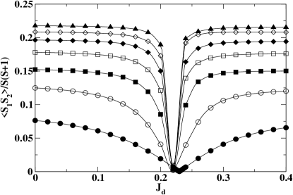
Figure 19: First neighbor correlation as function of $J_{d}$ and $S=\frac{1}{2}$ (circles), $S=1$ (squares), $S=\frac{3}{2}$ (diamonds), $S=2$ (triangles) $S=\frac{5}{2}$ (filled diamonds), $S=3$ (open diamonds), $S=\frac{7}{2}$, (filled triangles).

The tendency to the severing of the chains is more clearly seen in the transverse bond strength

$$C_{1}=\langle S_{5,6}^{z}S_{5,7}^{z}\rangle,$$ (13)

shown in Fig.(19). In all cases, $C_{1}$ decreases from its value at $J_{d}=0$ and seems to vanish at $J_{d}^{0}$ (we were able in all cases to reach values of $C_{1}$ which are equal or less than the numerical accuracy of in our simulations). From this point it increases. There is a small difference between the position of $J_{d}^{0}$ for different values of $S$ as found for $E_{G}$. The curves of $C_{1}$ suggest that for all $S$, the mechanism to avoid frustration is identical: the systems relaxe to nearly disconnected chains. These curves also show the influence of quantum fluctuations for small $S$. This is seen in the decay of $C_{1}$ as soon as $J_{d}\neq 0$. For larger $S$, $C_{1}$ remains nearly constant until $J_{d}\approx J_{d}^{0}$.

IV.3 Long-distance correlations

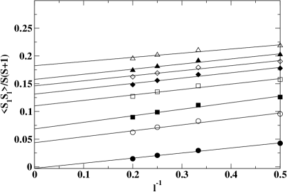
Figure 20: Spin-spin correlation at $J_{d}=0$ as function of $l$ and $S=\frac{1}{2}$ (filled circles), $S=1$ (open circles), $S=\frac{3}{2}$ (filled squares), $S=2$ (open squares), $S=\frac{5}{2}$ (filled diamonds), $S=3$ (open diamonds), $S=\frac{7}{2}$, (filled triangles), $S=4$ (open triangles).

Since our starting point for 2D systems is disconnected chains, it is important to show, as for the spin $1/2$ case studied previously, that the TSDMRG is able to reach the ordered phase. One possible way to look at the appearance of the ordered state is to look at the decay of the transverse correlation function,

$$C_{l}=\langle S_{5,6}^{z}S_{5,5+l}^{z}\rangle,$$ (14)

in the Néel phase for $J_{d}=0$. We found that for all values of $S$ except $S=\frac{1}{2}$, as shown in Fig.(20), the transverse correlation function extrapolate to finite values. $C_{l}$ extrapolates to a negative value for $S=\frac{1}{2}$. In that case, quantum fluctuations are so strong that it is necessary to go to larger values of $L$ as done in Ref.(moukouri-TSDMRG2 ).

At the maximally frustrated point, we also observe similar exponential decay of $C_{l}$ as for $S=\frac{1}{2}$. This decay is less faster with increasing $S$. Indeed in the limit $S\rightarrow\infty$, the transition is of first order. The chains are disconnected in this classical limit and $C_{l}$ is exactly equal to zero. However for any small deviation from the transition point, the system falls in one of the ordered states. This point is virtually impossible to find exactly numerically. However, for smaller values of $S$ the critical region is larger and even if we miss the exact transition point, this behavior will nevertheless be observed as far as we close enough to the QCP.

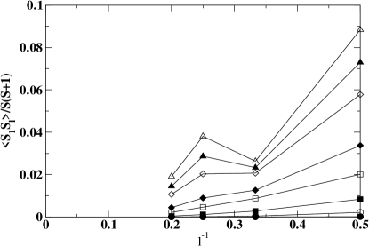
Figure 21: Transverse spin-spin correlation at $J_{d}=0.22$ as function of $l$ and $S=\frac{1}{2}$ (circles), $S=1$ (squares), $S=\frac{3}{2}$ (diamonds), $S=2$ (triangles), $S=\frac{5}{2}$ (filled diamonds), $S=3$ (open diamonds), $S=\frac{7}{2}$, (filled triangles), $S=4$ (open triangles).

IV.4 Spin gaps

The curves of $\Delta(J_{d})$ in Fig.(22) for different values of $S$ have typically a peak in the at $J_{d}=J_{d}^{max}$. This peak is very narrow, except for $S=\frac{1}{2}$ where quantum fluctuation effects lead to a broader peak. As expected from the behavior of $C_{1}$, this peak is sharper with increasing $S$. $\Delta(J_{d}^{max})$ is nearly equal to the finite size gap of an isolated chain which is represented by a flat line in each case. We were unable to reach the 1D gap for $S>\frac{3}{2}$. This is probably due to the narrowness of the critical region which makes it difficult to see the nearly disconnected chain regime. One can easily fall in one of the ordered regime leading to a relative slower decay of $C_{l}$ which manifests itself to a smaller finite size gap.

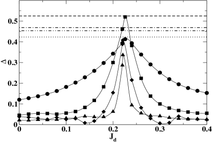
Figure 22: Spin gap as function of $J_{d}$ and $S=\frac{1}{2}$ (circles), $S=1$ (squares), $S=\frac{3}{2}$ (diamonds), $S=2$ (triangles)

.

IV.5 Conclusion

In this section, we presented results for $L=10$ and $J_{\perp}=0.4$ with $S$ varying from $\frac{1}{2}$ to $4$. In agreement with the DLS theorem, we found long-range order for all $S$ greater or equal to $1$ in the unfrustrated case. As $J_{d}$ is turned on, the long-range order is destroyed. An interesting question is the nature of this disordered state as function of $S$. Before addressing this question, we will first review how frustration works in 1D schollwock .

For the frustrated $S=\frac{1}{2}$ chain, there is a transition to a dimerized phase at $J_{2c}=0.242J_{1}$, where $J_{2c}$ is the value of next-nearest neighbor coupling at the critical point. At this point a gap opens exponentially and grows with $J_{2}$. At $J_{2}=0.5J_{1}$, the system is perfectly dimerized and shows incommensurate correlation above this point (disordered point). At about $J_{2}=0.52J_{1}$ a two-peak structure appears in the structure factor (Lifshitz point). DMRG simulations for the $S=\frac{3}{2}$ chain shows a similar behavior. This suggests that it is generic to half-integer spin systems.

Integer spin chains are already gapped in the absence of the frustration term $J_{2}$. For $S=1$, the transition to a dimerized phase is absent, but numerical simulations show the presence of the disordered and the Lifshitz points. In addition there is a first order transition at $J_{2}=0.75J_{1}$ from a phase with a single string order to a phase with a double string order. At this point the chain splits into two chains. These special points are also observed in the $S=2$ chain except that the order parameter for the first order transition is still unknown.

The results presented in the preceding sections show that the mechanism to ease frustration works differently in 2D systems. This mechanism is the same for all values of $S$. The system spontaneously severs the frustrated bond at the maximally frustrated point. The similarity for all $S$ of this mechanism stems from the fact that if the transverse coupling is large enough, all the 2D systems are ordered for half-integer as well as for odd integer systems. Frustration is a competition between two magnetic ground phases and we have shown that for coupled chain systems, the best way to avoid frustration is to relax into nearly independent chains. It is clear that such a mechanism will be independent on the value of the spin as found in our numerical study. The consequences are nevertheless different for half-odd integer and for integer spin systems.

For all spin half-odd integer systems, like for the spin $1/2$ studied more extensively in Ref.(moukouri-TSDMRG3 ), there is a second order phase transition between the two magnetic states at $J_{d}=J_{d}^{max}$. At the critical point, the system is disordered. The transverse correlation decay exponentially while at long distances, the longitudinal one behave like those of independent chains. Hence at the critical point, the spin rotational symmetry of the Hamiltonian is restored. As for spin $1/2$, there might be a residual interaction which can drive the system eventually to a SP phase. But, previous numerical studies on 2D systems moukouri-TSDMRG3 and on three-leg ladders point to an absence of a dimerized phase in this region for $S=\frac{1}{2}$. This is expected to be valid for all half-odd $S$. We would like to stress that dimerization is not the driving mechanism mechanism in the formation of the disordered state. We are indeed aware of earlier ED results dagotto in which an enhancement of the SP susceptibility was observed in the regime $J_{2}\approx J_{1}/2$. We believe in the light of our results that this merely the consequence of the severing of the chains in one of the two directions of the square lattice. The SP signal is expected to be larger in 1D where it has a power law decay than in 2D when the spins are locked into Néel order in the unfrustrated regime.

For integer spins, there is an intermediate phase between the two magnetic states. When $|J_{\perp}-2J_{d}|\ll\Delta$, where $\Delta$ is the single chain spin gap, the transverse coupling are irrelevant. The maximally frustrated point is the equivalent of the disordered point seen in 1D. In this regime of couplings, the system is an assembly of nearly decoupled chains. In the case of integer spins, even if there is a residual interaction at the maximally frustrated point, this interaction is necessary irrelevant because of the presence of $\Delta$. Integer spin systems are thus radically different from half-odd integer systems.

V Conclusion

In this paper, we used the TSDMRG to study coupled spin chains with $S$ varying from $\frac{1}{2}$ to $4$. This study illustrates the power of the TSDMRG method, where using a modest computer effort we were able to study the unfrustrated regime and find long-range magnetic order, in agreement with the DLS theorem and Monte Carlo studies. We obtained good accuracy in the highly frustrated regime of the model. The study of this region has so far resisted to other numerical methods.

We showed that in order to avoid frustration, all spin systems tend to sever the frustrated bonds. The severing of the transverse bonds is a large effect which is seen in various physical quantities. The strong frustration regime is dominated by 1D physics, topological effects become important as predicted in Ref.(affleck1 ; haldane2 ; read ). However, we did not find any qualitative difference between odd and even integer spin systems as predicted in Ref.(haldane2 ; read ). It could be due to the fact that in the highly frustrated regime the 2D systems tend to relax into nearly independent 1D sytems where tolological effects are identical for odd and even integer spins. It could also be related to the anisotropy of the model studied.

- (1) F. J. Dyson, E. H. Lieb, and B. Simon, J. Stat. Phys. 18, 335 (1978).
- (2) E. J. Neves and J. F. Peres, Phys. Lett. 114A, 331 (1986).
- (3) J. D. Reger and A. P. Young, Phys. Rev. B 37, 5978 (1988).
- (4) T. Dombre and N. Read, Phys. Rev. B 38, 7181 (1988).
- (5) E. Fradkin and M. Stone, Phys. Rev. B 38, 7215 (1988).
- (6) X.-G. Wen and A. Zee, Phys. Rev. Lett. 61, 1025 (1988).
- (7) F. D. M. Haldane, Phys. Rev. Lett. 61, 1029 (1988).
- (8) I. Affleck, Phys. Rev. B 37, 5186 (1988).
- (9) A. Vishwanath and D. Carpentier, Phys. Rev. Lett. 86, 676 (2001).
- (10) V.J Emery, E. Fradkin, S.A. Kivelson, and T.C. Lubensky, Phys. Rev. Lett. 85, 2160 (2000).
- (11) R. Mukhopadhyay, C.L. Kane, and T.C. Lubensky, Phys. Rev. B 64, 045120 (2001).
- (12) A. A. Nersesyan and A. M. Tsvelik Phys. Rev. B 67, 024422 (2003); A. M. Tsvelik Phys. Rev. B 70, 134412 (2004).
- (13) O. A. Starykh and L. Balents Phys. Rev. Lett. 93, 127202 (2004).
- (14) G. hager, E. Jeckelmann, H. Feske, and G. Wellein, J. Comp. Phys. 194, 795 (2004).
- (15) S. Moukouri and J.V. Alvarez cond-mat/0403372.
- (16) S.R. White, Phys. Rev. Lett. 69, 2863 (1992). Phys. Rev. B 48, 10 345 (1993).
- (17) G. Misguich and C. Lhuillier in ”Frustrated Spin Systems” Ed. H.T. Diep World Scientific (2004).
- (18) A. Sindzingre, Phys. Rev. B 69, 094418 (2004).
- (19) F. D. M. Haldane, Phys. Lett. 93A, 464 (1983); Phys. Rev. Lett. 50, 1153 (1983).
- (20) E. Lieb, T. Schultz, and D. Mattis, Ann. Phys. (N.Y.) 16, 407 (1961).
- (21) N. Read and S. Sachdev, Phys. Rev. Lett 66, 1773 (1991).
- (22) S. Moukouri, cond-mat/0504306 (unpublished).
- (23) E. Fradkin in ”Field Theories of Condensed Matter Systems”, Ed. D. Pines, West View Press (1991).
- (24) S. Moukouri and L.G. Caron, Phys. Rev. B 67, 092405 (2003).
- (25) S. Moukouri, Phys. Rev. B 70, 014403 (2004).
- (26) S. Moukouri, (unpublished).
- (27) J.V. Alvarez and S. Moukouri, Int. J. Mod. Phys. C 16, 843 (2005).
- (28) K. G. Wilson, Rev. Mod. Phys. 47, 773 (1975).
- (29) X. Wang, N. Zhu, C. Chen, Phys. Rev. B 66 172405 (2002).
- (30) I. Affleck and S. Qin, J. Phys. A 32, 7815 (1999).
- (31) E. Dagotto and A. Moreo, Phys. rev. Lett. 63, 2148 (1989).
- (32) I. Affleck and J.B Marston, Phys. Rev. B 37, 3774 (1988).
- (33) I. Affleck, T. Kennedy, E. H. Lieb, and H. Tasaka, Comm. Math. Phys. 115, 477 (1988).
- (34) X.-G. Wen, F. Wilczeck, and A. Zee, Phys. Rev. 39, 11413 (1989).
- (35) G. Kotliar, Phys. Rev. B 37, 3664 (1988).
- (36) G. Baskaran, Z. Zou, and P. W. Anderson, Sol. St. Comm. 63, 973 (1987).
- (37) T. Senthil, A. Vishwanath, L. Balents, S. Sachdev, and M. P. A. Fisher, Science 303, 1490 (2004).
- (38) R. Roth and U. Schollwöck, Phys. Rev. 58, 9264 (1998).