Manifestation of the Roughness-Square-Gradient Scattering
in Surface-Corrugated Waveguides

Abstract

We study a new mechanism of wave/electron scattering in multi-mode surface-corrugated waveguides/wires. This mechanism is due to specific square-gradient terms in an effective Hamiltonian describing the surface scattering, that were neglected in all previous studies. With a careful analysis of the role of roughness slopes in a surface profile, we show that these terms strongly contribute to the expression for the inverse attenuation length (mean free path), provided the correlation length of corrugations is relatively small. The analytical results are illustrated by numerical data.

I Introduction

The subject of wave transport through guiding surface-disordered systems is of great importance in various physical applications. Recently, this topic has attracted even more attention due to a burst of developments in nano-science where frequently one deals with devices or structures (quantum wires, leads, etc.) whose surface’s irregularities become more important than those in the bulk. Other situations for either electromagnetic or acoustic waves (remote sensing, photonic and acoustic devices, optical thin films, etc.) are analogous. Therefore, in what follows we do not make any distinction between electromagnetic/electron or any other type of waves.

In spite of an extensive research of unitary wave scattering from rough surfaces, the problem of transport in the waveguides with such profiles still remains open. This problem is a great theoretical challenge since it deals with the multiple scattering of a wave from lateral walls. As a result of this scattering, the unperturbed longitudinal wave number $k_{n}$ of an $n$-th propagating normal mode changes, $k_{n}\to k_{n}+\delta k_{n}$, due to a complex amount $\delta k_{n}$,

$$\delta k_{n}=\gamma_{n}+i(2L_{n})^{-1}.$$ (1)

The real part $\gamma_{n}$ is responsible for the roughness-induced correction to the phase velocity, while $L_{n}$ is the electron total mean free path, scattering length or attenuation length of a given mode. As is known, the shift $\gamma_{n}$ does not change the static transport of a disordered systems. Therefore, our further analysis shall be focused only on the attenuation length $L_{n}$.

Evidently, statistical properties of a rough surface profile $\xi(x)$ give a strong impact on the scattering process. However, a proper incorporation of these properties into the theory accounting for the guided and scattered waves, is not a trivial task. Many approaches have been proposed in connection with the surface scattering (see, e.g., Refs. BFb79, ; RytKrTat89, ; VoronB94, ; SMFY98, ; SFMY99, ; Konrady74, ; McGM84, ; TJM86, ; TrAsh88, ; IsPuzFuks9091, ; Tatar93, ; KMYa91, ; MakMorYam95, ; MT9801, ; MeyStep949597989900, ; LunKyReiKr96, ; BratRash96, ; LunMenIz01, and references therein). One of the main tools to treat this problem is a reduction of the surface scattering to the bulk one in such a way that the latter can be formally described by an effective Hamiltonian $\widehat{H}$,

$$\widehat{H}^{(0)}\to\widehat{H}=\widehat{H}^{(0)}+\widehat{U},$$ (2)

with flat boundaries, however, with a complicated potential $\widehat{U}$. To the best of our knowledge, originally the idea of this approach was discussed by Migdal Mig77 . After, it was frequently used in the theories of classical and quantum wave scattering, see, e.g., Refs. Konrady74, ; TJM86, ; TrAsh88, ; BratRash96, ; MeyStep949597989900, ; LunKyReiKr96, ; IsPuzFuks9091, ; MT9801, ; LunMenIz01, . One should stress that in the majority of them Konrady74 ; TJM86 ; TrAsh88 ; MeyStep949597989900 ; LunKyReiKr96 ; BratRash96 the study was restricted to the lowest order in the root-mean-square roughness height $\sigma$. Other methods IsPuzFuks9091 ; MT9801 ; LunMenIz01 ; VoronB94 ; KMYa91 ; MakMorYam95 ; Tatar93 were mainly based on a principal assumption that the surface roughness is sufficiently smooth.

In this paper we present analytical results demonstrating a new scattering mechanism missed in previous studies of the surface scattering. This mechanism is due to specific square-gradient (SG) terms that are proportional to $\sigma^{2}{\xi^{\prime}}^{2}(x)$ in the potential $\widehat{U}$. We argue that the discovered scattering mechanism is substantially different from the known ones associated with the roughness amplitude and roughness gradient of the surface.

The two last mechanisms have been already studied (see, e.g. Refs. BFb79, ; MeyStep949597989900, ; LunKyReiKr96, ). Their main contributions were shown to depend on the terms containing the quantities $\sigma\xi(x)$ and $\sigma\xi^{\prime}(x)$, respectively. In the performed analysis the square-gradient terms related with the new scattering mechanism were discarded due their seemingly small contribution. Indeed, the square-gradient terms are formally proportional to $\sigma^{2}$, similar to other terms that arise in the next (second-order) approximation in the amplitude and gradient roughness. However, we have found that the square-gradient terms have a very strong dependence on the roughness correlation length $R_{c}$, in contrast with those terms appearing in the second-order approximation. Specifically, with a decrease of $R_{c}$ the square-gradient terms in the expression for the mean free path compete with the standard terms proportional to $\sigma\xi(x)$ and $\sigma\xi^{\prime}(x)$.

One should stress that our approach is restricted by the first order approximation, with a careful analysis of all terms that may be important in this approximation, and taking into account an unexpectedly strong influence of the square-gradient terms. Our goal is to study the new scattering mechanism and establish the conditions when it should not be neglected. For this, we derive a correct expression for the attenuation length $L_{n}$ that incorporates the contribution of the above mechanism. One should emphasize that the approach we use does not assume any special restrictions to the model parameters (such as the smoothness of surface profiles) except for general conditions of weak scattering.

The paper is organized as follows. In Sec. II we formulate the problem and discuss the coordinate transformation used to represent the surface scattering as the bulk one. Our approach involves an average Green’s function whose longitudinal wave number is a modification of the unperturbed one. Also, all expressions corresponding to the unperturbed problem are given and discussed in this Section. In Sec. III we derive a Dyson-type integral equation for the exact Green’s function. From the exact expression for the scattering potential we design two Hermitian random operators. The first one is associated with both the amplitude (AS) and the gradient scattering (GS) mechanism, while the second one is associated only with the square-gradient scattering (SGS) mechanism. The former operator gives rise to the roughness-height power (RHP) spectrum $W(k_{x})$, while the latter to the roughness-square-gradient power (RSGP) spectrum $T(k_{x})$.

In Sec. IV we obtain the averaged Green’s function by applying a perturbative method with respect to the above operators. Since in this work we restrict ourselves to the analysis of the attenuation length $L_{n}$ of the $n$-th conducting mode, we focus our attention to the imaginary part of the proper self-energy. In Sec. V, in correspondence with a clear independence between AS+GS and SGS mechanisms, we develop a natural approach to define two attenuation lengths, the well known one, $L_{n}^{(1)}$, and the new SGS length $L_{n}^{(2)}$. These two lengths are related to the RHP and the RSGP spectrum, and, as a consequence, they are characterized by $\sigma^{2}$ and $\sigma^{4}$ dependencies, respectively. We study their interplay for two limit cases of the roughness surface, for small-scale and large-scale roughness. We discuss here the main result according to which the larger roughness slope $\sigma/R_{c}$, the larger contribution of the SGS mechanism. We also present a numerical analysis assuming that the surface profile $\xi(x)$ has the standard Gaussian binary correlator. Finally, in Section VI we outline our conclusions. A short presentation of main results can be found in Ref. IzMakRen05, .

II Problem formulation

In what follows, we consider an open plane waveguide (or conducting quasi-one-dimensional wire) of average width $d$, stretched along the $x$-axis. For simplicity, one (lower) surface of the waveguide is assumed to be flat, $z=0$, while the other (upper) surface has a rough profile, $z=d+\sigma\xi(x)$, with $\sigma$ as the root-mean-square roughness height. In other words, the waveguide occupies the region

$$-\infty\leq x\leq\infty,\qquad\qquad 0\leq z\leq w(x)$$ (3)

of the $(x,z)$-plane. Here the fluctuating wire width $w(x)$ is defined by

$$w(x)=d+\sigma\xi(x),\qquad\qquad\langle w(x)\rangle=d.$$ (4)

The random function $\xi(x)$ describes the roughness of the upper boundary. It is assumed to be a statistically homogeneous and isotropic Gaussian random process with the zero mean and unit variance,

$$\langle\xi(x)\rangle=0,\quad\langle\xi^{2}(x)\rangle=1,\quad\langle\xi(x)\xi(x^{\prime})\rangle={\cal W}(x-x^{\prime}).$$ (5)

Here the angular brackets stand for statistical averaging over different realizations of the surface profile $\xi(x)$. We also assume that its binary correlator ${\cal W}(x)$ decreases on the scale $R_{c}$ and is normalized to one, ${\cal W}(0)=1$.

The roughness-height power (RHP) spectrum $W(k_{x})$ is defined by

$$W(k_{x})=\int_{-\infty}^{\infty}dx\exp(-ik_{x}x)\,{\cal W}(x).$$ (6)

Since ${\cal W}(x)$ is an even function of $x$, its Fourier transform (6) is even, real and non-negative function of $k_{x}$. The RHP spectrum has maximum at $k_{x}=0$ with $W(0)\sim R_{c}$, and decreases on the scale $R_{c}^{-1}$.

In order to analyze the surface scattering problem we shall employ the method of retarded Green’s function ${\cal G}(x,x^{\prime};z,z^{\prime})$. Specifically, we start with the Dirichlet boundary-value problem

$$\left(\frac{\partial^{2}}{\partial x^{2}}+\frac{\partial^{2}}{\partial z^{2}}+k^{2}\right){\cal G}(x,x^{\prime};z,z^{\prime})$$

$$=\delta(x-x^{\prime})\delta(z-z^{\prime}),$$ (7a)

$${\cal G}(x,x^{\prime};z=0,z^{\prime})=0,$$

$${\cal G}(x,x^{\prime};z=d+\sigma\xi(x),z^{\prime})=0.$$ (7b)

Here $\delta(x)$ and $\delta(z)$ are the Dirac delta-functions. The wave number $k$ is equal to $\omega/c$ for an electromagnetic wave of the frequency $\omega$ and TE polarization, propagating through a waveguide with perfectly conducting walls. For an electron quantum wire, $k$ is the Fermi wave number within the isotropic Fermi-liquid model.

II.1 Coordinate transformation

The equation (7a) does not contain any scattering potential. In contrast with the bulk scattering, the electromagnetic/electron waves experience a perturbation due to scattering from the upper wall, therefore, the perturbation is hidden in the boundary condition (7b). In order to formally describe the surface scattering as a bulk one, we perform the canonical transformation to new coordinates,

$$x_{new} = x_{old},$$ (8a)

$$z_{new} = \frac{d}{w(x)}z_{old}=\frac{d}{d+\sigma\xi(x)}z_{old},$$ (8b)

in which both waveguide surfaces are flat. Correspondingly, we introduce the canonically conjugate Green’s function (below for convenience we drop the subscript “new” for $x$ and $z$),

$${\cal G}_{new}(x,x^{\prime};z,z^{\prime})=\frac{\sqrt{w(x)w(x^{\prime})}}{d}\,{\cal G}_{old}(x,x^{\prime};z,z^{\prime}).$$ (9)

As a result, we arrive at the equivalent boundary-value problem governed by the equation

$$\Bigg{(}\frac{\partial^{2}}{\partial x^{2}}+\frac{\partial^{2}}{\partial z^{2}}+k^{2}\Bigg{)}\,{\cal G}(x,x^{\prime};z,z^{\prime})$$

$$-\widehat{U}(x,z)\,{\cal G}(x,x^{\prime};z,z^{\prime})=\delta(x-x^{\prime})\delta(z-z^{\prime}),\qquad$$ (10a)

$${\cal G}(x,x^{\prime};z=0,z^{\prime})=0,$$

$${\cal G}(x,x^{\prime};z=d,z^{\prime})=0.$$ (10b)

Here the effective surface scattering potential $\widehat{U}(x,z)$ is given by the following expression,

$$\widehat{U}(x,z) = \bigg{[}1-\frac{d^{2}}{w^{2}(x)}\bigg{]}\frac{\partial^{2}}{\partial z^{2}}$$ (11)

$$+ \frac{\sigma}{w(x)}\left[\xi^{\prime\prime}(x)+2\xi^{\prime}(x)\frac{\partial}{\partial x}\right]\left[\frac{1}{2}+z\frac{\partial}{\partial z}\right]$$

$$- \frac{\sigma^{2}{\xi^{\prime}}^{2}(x)}{w^{2}(x)}\left[\frac{3}{4}+3z\frac{\partial}{\partial z}+z^{2}\frac{\partial^{2}}{{\partial z}^{2}}\right].$$

Note that the prime over the function $\xi(x)$ denotes a derivative with respect to $x$. It is important to stress that Eqs. (10)–(11) are exact and valid for any form of the surface profile $\xi(x)$.

II.2 Unperturbed Green’s function

The unperturbed Green’s function ${\cal G}_{0}(|x-x^{\prime}|;z,z^{\prime})$ obeys the boundary-value problem (10) with $\widehat{U}(x,z)=0$ (when $\sigma=0$, and therefore, $w(x)=d$). It is determined as follows,

$${\cal G}_{0}(|x-x^{\prime}|;z,z^{\prime})=\int_{-\infty}^{\infty}\frac{dk_{x}dk_{x}^{\prime}}{(2\pi)^{2}}\,\exp\left[i(k_{x}x-k_{x}^{\prime}x^{\prime})\right]$$

$$\times g_{0}(k_{x},k_{x}^{\prime})\,\frac{\sin(k_{z}z)\sin(k_{z}^{\prime}z^{\prime})}{k_{z}k_{z}^{\prime}}$$ (12a)

$$=\sum_{n=1}^{N_{d}}\sin\left(\frac{\pi nz}{d}\right)\sin\left(\frac{\pi nz^{\prime}}{d}\right)\frac{\exp\left(ik_{n}|x-x^{\prime}|\right)}{ik_{n}d}.\qquad\quad$$ (12b)

Here $k_{x}$ and $k_{z}$ are the lengthwise and transverse wave numbers,

$$k_{z}=k_{z}(k_{x})=\sqrt{k^{2}-k_{x}^{2}},\qquad k_{z}^{\prime}=k_{z}(k_{x}^{\prime}).$$ (13)

Their unperturbed eigenvalues are $k_{n}$,

$$k_{n}=\sqrt{k^{2}-(\pi n/d)^{2}},\qquad n=1,2,3,\ldots,N_{d},$$ (14)

and $\pi n/d$ respectively. The total number $N_{d}$ of propagating waveguide modes (conducting channels that have real values of $k_{n}$) is determined by the integer part $[\ldots]$ of the ratio $kd/\pi$,

$$N_{d}=[kd/\pi].$$ (15)

The first expression (12a) gives the unperturbed Green’s function in the pole representation where $g_{0}(k_{x},k_{x}^{\prime})$ is called the pole factor,

$$g_{0}(k_{x},k_{x}^{\prime})=2\pi\delta(k_{x}-k_{x}^{\prime})\,g_{0}(k_{x}),$$ (16a)

$$g_{0}(k_{x})=k_{z}\cot(k_{z}d)\,\to$$ (16b)

$$\sum_{n=1}^{N_{d}}\frac{(\pi n/d)^{2}}{k_{n}d}\left(\frac{1}{k_{x}+k_{n}+i0}-\frac{1}{k_{x}-k_{n}-i0}\right).\qquad\quad$$ (16c)

The evaluation of the integrals in Eq. (12a) over the poles of $g_{0}(k_{x},k_{x}^{\prime})$, results in the mode representation (12b) for the unperturbed Green’s function.

III Dyson Equation

With the use of the Green’s theorem, it can be easily shown that the boundary-value problem (10) is directly reduced to the following exact Dyson-type integral equation

$${\cal G}(x,x^{\prime};z,z^{\prime})={\cal G}_{0}(|x-x^{\prime}|;z,z^{\prime})+\int_{-\infty}^{\infty}dx_{1}\int_{0}^{d}dz_{1}$$

$${\cal G}_{0}(|x-x_{1}|;z,z_{1})\,\widehat{U}(x_{1},z_{1})\,{\cal G}(x_{1},x^{\prime};z_{1},z^{\prime}).\qquad$$ (17)

This equation relates the perturbed by surface disorder Green’s function ${\cal G}(x,x^{\prime};z,z^{\prime})$ to the Green’s function ${\cal G}_{0}(|x-x^{\prime}|;z,z^{\prime})$ of the waveguide with perfectly flat boundaries.

Similarly to the pole representation (12a) for the unperturbed Green’s function, let us seek ${\cal G}(x,x^{\prime};z,z^{\prime})$ in the form

$${\cal G}(x,x^{\prime};z,z^{\prime})=\int_{-\infty}^{\infty}\frac{dk_{x}dk_{x}^{\prime}}{(2\pi)^{2}}\exp\left[i(k_{x}x-k_{x}^{\prime}x^{\prime})\right]$$

$$\times g(k_{x},k_{x}^{\prime})\,\frac{\sin(k_{z}z)\sin(k_{z}^{\prime}z^{\prime})}{k_{z}k_{z}^{\prime}}.$$ (18)

With this method the problem of deriving the Green’s function ${\cal G}(x,x^{\prime};z,z^{\prime})$ is reduced to obtain its pole factor $g(k_{x},k_{x}^{\prime})$. To this end, we substitute the pole representations (12a) and (18) into Eq. (17) and get the non-local Dyson equation in the $k_{x}$-representation,

$$g(k_{x},k_{x}^{\prime})=g_{0}(k_{x},k_{x}^{\prime})$$

$$+\int_{-\infty}^{\infty}\frac{dq_{x}dq_{x}^{\prime}}{(2\pi)^{2}}g_{0}(k_{x},q_{x})\Xi(q_{x},q_{x}^{\prime})g(q_{x}^{\prime},k_{x}^{\prime}).\qquad\qquad$$ (19)

In this representation the effective surface scattering potential $\Xi(k_{x},k^{\prime}_{x})$ is

$$\Xi(k_{x},k^{\prime}_{x})=\int_{-\infty}^{\infty}dx_{1}\int_{0}^{d}dz_{1}\,\exp\left(-ik_{x}x_{1}\right)\frac{\sin(k_{z}z_{1})}{k_{z}}$$

$$\times\widehat{U}(x_{1},z_{1})\;\exp\left(ik^{\prime}_{x}x_{1}\right)\frac{\sin(k^{\prime}_{z}z_{1})}{k^{\prime}_{z}}\,.$$ (20)

Thus, we obtained the Dyson-type integral equation (19) with an exact expression (20) for the kernel $\Xi(k_{x},k^{\prime}_{x})$. After the substitution of the expression (11) for $\widehat{U}$, we realize that the kernel consists of three groups of terms. The first one has the factor $(1-d^{2}/w^{2}(x_{1}))$ while the second and third group has, respectively, the factor $\sigma/w(x_{1})$ and $\sigma^{2}/w^{2}(x_{1})$. One needs to note that while the kernel $\Xi(k_{x},k^{\prime}_{x})$ is Hermitian in the whole, its latter two parts are non-Hermitian individually. To have each part of $\Xi(k_{x},k^{\prime}_{x})$ Hermitian, we perform the integration by parts for the term containing $\xi^{\prime\prime}(x_{1})$ in the second group. After that we come to the final exact form for the perturbation potential,

$$\Xi(k_{x},k^{\prime}_{x})=\int_{-\infty}^{\infty}dx_{1}\int_{0}^{d}dz_{1}\,\exp\left(-ik_{x}x_{1}\right)\frac{\sin(k_{z}z_{1})}{k_{z}}$$

$$\times\left\{\left[1-\frac{d^{2}}{w^{2}(x_{1})}\right]\frac{\partial^{2}}{\partial z_{1}^{2}}\right.$$

$$+\,i(k_{x}+k_{x}^{\prime})\frac{\sigma\xi^{\prime}(x_{1})}{w(x_{1})}\left[\frac{1}{2}+z_{1}\frac{\partial}{\partial z_{1}}\right]$$

$$-\left.\frac{\sigma^{2}{\xi^{\prime}}^{2}(x_{1})}{w^{2}(x_{1})}\left[\frac{1}{4}+2z_{1}\,\frac{\partial}{\partial z_{1}}+z_{1}^{2}\frac{\partial^{2}}{\partial z_{1}^{2}}\right]\right\}$$

$$\times\exp\left(ik^{\prime}_{x}x_{1}\right)\frac{\sin(k^{\prime}_{z}z_{1})}{k^{\prime}_{z}}.$$ (21)

This equation has a peculiar structure very useful in further analysis. The kernel written in this form also consists of three groups of terms, however, now they represent different scattering mechanisms.

Since we are interested in the averaged Green’s function, we have to calculate the binary correlator of $\Xi(k_{x},k^{\prime}_{x})$. Therefore, to avoid very cumbersome calculations, it is reasonable to make a simplification of $\Xi(k_{x},k^{\prime}_{x})$ that does not destroy the Hermitian structure of each group of terms. To this end, and taking into account that our interest is in the typical case of small surface corrugations ($\sigma\ll d$), we can do the following: expand the factor $1-d^{2}/w^{2}(x_{1})\approx 2\sigma\xi(x_{1})/d$ in the first term of Eq. (21) and put $w(x_{1})\approx d$ in all the others. In such a way, we get a suitable approximate expression for the surface scattering potential,

$$\Xi(k_{x},k^{\prime}_{x})\approx\int_{-\infty}^{\infty}dx_{1}\int_{0}^{d}dz_{1}\,\exp\left(-ik_{x}x_{1}\right)\frac{\sin(k_{z}z_{1})}{k_{z}}$$

$$\times\left\{\frac{2\sigma\xi(x_{1})}{d}\frac{\partial^{2}}{\partial z_{1}^{2}}+i(k_{x}+k_{x}^{\prime})\frac{\sigma\xi^{\prime}(x_{1})}{d}\left[\frac{1}{2}+z_{1}\frac{\partial}{\partial z_{1}}\right]\right.$$

$$-\left.\frac{\sigma^{2}{\xi^{\prime}}^{2}(x_{1})}{d^{2}}\left[\frac{1}{4}+2z_{1}\,\frac{\partial}{\partial z_{1}}+z_{1}^{2}\frac{\partial^{2}}{\partial z_{1}^{2}}\right]\right\}$$

$$\times\exp\left(ik^{\prime}_{x}x_{1}\right)\frac{\sin(k^{\prime}_{z}z_{1})}{k^{\prime}_{z}}.$$ (22)

The expression (22) contains one term that depends on the amplitude of the roughness profile $\sigma\xi(x_{1})$, and two groups of terms that depend on the roughness gradient $\sigma\xi^{\prime}(x_{1})$ and the roughness square-gradient $\sigma^{2}{\xi^{\prime}}^{2}(x_{1})$ terms, respectively. An interesting point to mention is that the last group, due to its proportionality to $\sigma^{2}$, was neglected in all previous studies of transport properties of surface-disordered waveguides. However, as we show below, the scattering due to these terms has the properties very different from those described by other terms, and should be properly taken into account.

In order to proceed further, we assert that the kernel can be written as the sum of its average, $\langle\Xi(k_{x},k^{\prime}_{x})\rangle$, and fluctuating, $\widetilde{\Xi}(k_{x},k^{\prime}_{x})$, parts, i.e.,

$$\Xi(k_{x},k^{\prime}_{x})=\langle\Xi(k_{x},k^{\prime}_{x})\rangle+\widetilde{\Xi}(k_{x},k^{\prime}_{x}).$$ (23)

It can be tested that the average, $\langle\Xi(k_{x},k^{\prime}_{x})\rangle$, contributes only to the real part $\gamma_{n}$ of the complex renormalization $\delta k_{n}$ of the lengthwise wave number $k_{n}$ (see Eq. (1)), and therefore, does not change static transport properties of the surface disordered waveguide. Thus, we will omit it because our interest is in the attenuation length $L_{n}$, not in $\gamma_{n}$.

From Eq. (22) one can see that all terms with the linear dependence on $\sigma$ have zero mean-value. Therefore, the average part $\langle\Xi(k_{x},k^{\prime}_{x})\rangle$ of the kernel $\Xi(k_{x},k^{\prime}_{x})$ is associated only with the group of terms containing $\sigma^{2}{\xi^{\prime}}^{2}(x_{1})$. To extract their fluctuating contribution, we should subtract from ${\xi^{\prime}}^{2}(x_{1})$ its mean value, $\langle{\xi^{\prime}}^{2}(x_{1})\rangle$. In such a way, we introduce the following zero-mean-valued operator

$$\widehat{\cal V}(x)={\xi^{\prime}}^{2}(x)-\langle{\xi^{\prime}}^{2}(x)\rangle\,,\qquad\langle\widehat{\cal V}(x)\rangle=0.$$ (24)

The operator $\widehat{\cal V}(x)$ plays a special role in our further consideration. In accordance with the Gaussian nature of the surface-profile function $\xi(x)$, the operator $\widehat{\cal V}(x)$ is uncorrelated with both $\xi(x)$ and $\xi^{\prime}(x)$,

$$\langle\xi(x)\widehat{\cal V}(x^{\prime})\rangle=0\,,\qquad\langle\xi^{\prime}(x)\widehat{\cal V}(x^{\prime})\rangle=0.$$ (25)

Its pair correlator is given by

$$\langle{\widehat{\cal V}(x)}{\widehat{\cal V}(x^{\prime})}\rangle=2\langle\xi^{\prime}(x)\xi^{\prime}(x^{\prime})\rangle^{2}=2{{\cal W}^{\prime\prime}}^{2}(x-x^{\prime}).$$ (26)

Since we use the $k_{x}$-representation, it is worthwhile to define the Fourier transform of the operator ${\widehat{\cal V}(x)}$,

$$V(k_{x}) = \int_{-\infty}^{\infty}dx\exp(-ik_{x}x)\widehat{\cal V}(x).$$ (27)

Also, we need the correlator of its Fourier transform,

$$\langle V(k_{x})V(k_{x}^{\prime})\rangle=4\pi\delta(k_{x}+k_{x}^{\prime})\,T(k_{x}).$$ (28)

Here the roughness-square-gradient power (RSGP) spectrum $T(k_{x})$ is

$$T(k_{x})=\int_{-\infty}^{\infty}dx\exp{(-ik_{x}x)}{{\cal W}^{\prime\prime}}^{2}(x).$$ (29)

One should stress that on the one hand, through the integration by parts, the power spectrum of the roughness gradients $\xi^{\prime}(x)$ can be reduced to the RHP spectrum $W(k_{x})$. On the other hand, it is not possible to do the same for the RSGP spectrum $T(k_{x})$. This very fact reflects a highly non-trivial role of the square-gradient scattering (SGS), giving rise to its competition with the well known scattering mechanism, in spite of the seeming smallness of the term $\sigma^{2}{\xi^{\prime}}^{2}(x)$.

With the introduction of $V(k_{x})$ we are ready to explicitly write down the fluctuating part of the total scattering potential,

$$\widetilde{\Xi}(k_{x},k_{x}^{\prime})=\Xi_{1}(k_{x},k_{x}^{\prime})+\Xi_{2}(k_{x},k_{x}^{\prime}).$$ (30)

The first summand is associated with the first and second terms in Eq. (22),

$$\Xi_{1}(k_{x},k_{x}^{\prime})=\int_{-\infty}^{\infty}dx_{1}\int_{0}^{d}dz_{1}\exp(-ik_{x}x_{1})\,\frac{\sin(k_{z}z_{1})}{k_{z}}$$

$$\times\left\{\frac{2\sigma\xi(x_{1})}{d}\frac{\partial^{2}}{\partial z_{1}^{2}}+i(k_{x}+k_{x}^{\prime})\frac{\sigma\xi^{\prime}(x_{1})}{d}\left[\frac{1}{2}+z_{1}\frac{\partial}{\partial z_{1}}\right]\right\}$$

$$\times\exp(ik_{x}^{\prime}x_{1})\,\frac{\sin(k_{z}^{\prime}z_{1})}{k_{z}^{\prime}}$$ (31a)

$$=-\sigma[A(k_{x},k_{x}^{\prime})+B(k_{x},k_{x}^{\prime})]\widetilde{\xi}(k_{x}-k_{x}^{\prime}).$$ (31b)

The second summand is related to the third term in Eq. (22), with ${\xi^{\prime}}^{2}(x_{1})$ being replaced by $\widehat{\cal V}(x_{1})$,

$$\Xi_{2}(k_{x},k_{x}^{\prime})=-\int_{-\infty}^{\infty}dx_{1}\int_{0}^{d}dz_{1}\exp(-ik_{x}x_{1})\frac{\sin(k_{z}z_{1})}{k_{z}}$$

$$\times\frac{\sigma^{2}\widehat{\cal V}(x_{1})}{d^{2}}\left[\frac{1}{4}+2z_{1}\,\frac{\partial}{\partial z_{1}}+z_{1}^{2}\frac{\partial^{2}}{\partial z_{1}^{2}}\right]$$

$$\times\exp(ik_{x}^{\prime}x_{1})\frac{\sin(k_{z}^{\prime}z_{1})}{k_{z}^{\prime}}$$ (32a)

$$=\sigma^{2}D(k_{x},k_{x}^{\prime})V(k_{x}-k_{x}^{\prime}).$$ (32b)

In Eq. (31) the quantity $\widetilde{\xi}(k_{x})$ is the Fourier transform of the function $\xi(x)$,

$$\widetilde{\xi}(k_{x}) = \int_{-\infty}^{\infty}dx\,\exp(-ik_{x}x)\,\xi(x).$$ (33)

Also, we have introduced the following quantities in the first summand:

$$A(k_{x},k_{x}^{\prime})=\frac{2k_{z}^{\prime}}{k_{z}d}\int_{0}^{d}dz\,\sin(k_{z}z)\sin(k_{z}^{\prime}z),\qquad\qquad$$ (34a)

$$A(\pm k_{n},\pm k_{n^{\prime}})=\delta_{nn^{\prime}}\,.$$ (34b)

$$B(k_{x},k_{x}^{\prime})=\frac{k_{x}^{2}-k_{x}^{\prime 2}}{d}\int_{0}^{d}dz\,\frac{\sin(k_{z}z)}{k_{z}}$$

$$\times\left[\frac{1}{2}+z\frac{\partial}{\partial z}\right]\frac{\sin(k_{z}^{\prime}z)}{k_{z}^{\prime}}\,,$$ (35a)

$$B(\pm k_{n},\pm k_{n^{\prime}})=\cos[\pi(n-n^{\prime})](1-\delta_{nn^{\prime}}).\qquad\qquad$$ (35b)

In the last expression we have used the equality

$$k_{x}^{2}-{k_{x}^{\prime}}^{2}=-(k_{z}^{2}-{k_{z}^{\prime}}^{2})$$ (36)

that directly follows from the energy conservation $k^{2}=k_{x}^{2}+k_{z}^{2}={k_{x}^{\prime}}^{2}+{k_{z}^{\prime}}^{2}$ (see the definition (13)). And finally, in the second summand the following factors appeared,

$$D(k_{x},k_{x}^{\prime})=-\frac{1}{d^{2}}\int_{0}^{d}dz\,\frac{\sin(k_{z}z)}{k_{z}}$$

$$\times\left[\frac{1}{4}+2z\,\frac{\partial}{\partial z}+z^{2}\frac{\partial^{2}}{\partial z^{2}}\right]\frac{\sin(k_{z}^{\prime}z)}{k_{z}^{\prime}}\,,$$ (37a)

$$D(\pm k_{n},\pm k_{n^{\prime}})=\frac{d}{2}\left[\frac{1}{3}+\frac{1}{(2\pi n)^{2}}\right]\delta_{nn^{\prime}}$$

$$+\frac{2d}{\pi^{2}}\,\frac{n^{2}+n^{\prime 2}}{(n^{2}-n^{\prime 2})^{2}}\,\cos[\pi(n-n^{\prime})](1-\delta_{nn^{\prime}}).\qquad\qquad$$ (37b)

The operator $\widetilde{\Xi}(k_{x},k_{x}^{\prime})$ written as the sum (30) of specially designed terms, has a very convenient form. First, both terms are chosen to have zero average. Second, since the operators $\xi(x)$ and $\widehat{\cal V}(x)$ do not correlate with each other (see Eq. (25)), their Fourier transforms are also uncorrelated,

$$\langle\tilde{\xi}(k_{x})V(k_{x}^{\prime})\rangle=0.$$ (38)

Due to the condition (38), the scattering potentials $\Xi_{1}(k_{x},k_{x}^{\prime})$ and $\Xi_{2}(k_{x},k_{x}^{\prime})$ are also uncorrelated. However, they have the following autocorrelators

$$\langle\Xi_{1}(k_{x},q_{x})\Xi_{1}(q_{x},k_{x}^{\prime})\rangle=$$

$$\qquad\qquad\qquad 2\pi\delta(k_{x}-k_{x}^{\prime})\,Q_{1}(k_{x},q_{x}),$$ (39a)

$$Q_{1}(k_{x},q_{x})=\sigma^{2}W(k_{x}-q_{x})\,[A(k_{x},q_{x})+B(k_{x},q_{x})]\quad$$

$$\qquad\qquad\times[A(q_{x},k_{x})+B(q_{x},k_{x})]\,.$$ (39b)

$$\langle\Xi_{2}(k_{x},q_{x})\Xi_{2}(q_{x},k_{x}^{\prime})\rangle=$$

$$\qquad\qquad\qquad 2\pi\delta(k_{x}-k_{x}^{\prime})\,Q_{2}(k_{x},q_{x}),\qquad$$ (40a)

$$Q_{2}(k_{x},q_{x})=2\sigma^{4}T(k_{x}-q_{x})$$

$$\qquad\qquad\times D(k_{x},q_{x})D(q_{x},k_{x})\,.$$ (40b)

As a result, the correlator of the fluctuating scattering potential (30) in the $k_{x}$-representation, is as follows

$$\langle\widetilde{\Xi}(k_{x},q_{x})\widetilde{\Xi}(q_{x},k_{x}^{\prime})\rangle=2\pi\delta(k_{x}-k_{x}^{\prime})Q(k_{x},q_{x}),\qquad\quad$$ (41a)

$$Q(k_{x},q_{x})=Q_{1}(k_{x},q_{x})+Q_{2}(k_{x},q_{x})\,.$$ (41b)

It is now possible to perform an appropriate perturbative averaging of the Dyson equation (19), and at the same time, to separate a relative contribution of the SGS mechanism from the total scattering process.

IV Average Green’s Function

Now we are in a position to replace the problem for the random Green’s function ${\cal G}(x,x^{\prime};z,z^{\prime})$ with the problem for the Green’s function $\langle{\cal G}(x,x^{\prime};z,z^{\prime})\rangle$ averaged over the surface disorder. It is evident that $\langle{\cal G}(x,x^{\prime};z,z^{\prime})\rangle$ is governed by Eq. (18) with the average pole factor $\langle g(k_{x},k_{x}^{\prime})\rangle$ instead of the random one. To perform the averaging of Eq. (19) with $\Xi(k_{x},k_{x}^{\prime})$ given by Eq. (30) and obtain $\langle g(k_{x},k_{x}^{\prime})\rangle$, we can apply one of the standard and well known perturbative methods. For example, it can be the diagrammatic approach developed for surface disordered systems BFb79 , as well as the technique developed in Ref. McGM84, . Both of the methods allow one to develop the consistent perturbative approach with respect to the scattering potential, that takes adequately into account the multiple scattering from the corrugated boundary. Then, we come to the following result

$$\langle g(k_{x},k_{x}^{\prime})\rangle=g_{0}(k_{x},k_{x}^{\prime})$$ (42)

$$+ \int_{-\infty}^{\infty}\frac{dq_{x}dq_{x}^{\prime}dq_{x}^{\prime\prime}dq_{x}^{\prime\prime\prime}}{(2\pi)^{4}}\,g_{0}(k_{x},q_{x})$$

$$\times \langle\widetilde{\Xi}(q_{x},q_{x}^{\prime})g_{0}(q_{x}^{\prime},q_{x}^{\prime\prime})\widetilde{\Xi}(q_{x}^{\prime\prime},q_{x}^{\prime\prime\prime})\rangle\langle g(q_{x}^{\prime\prime\prime},k_{x}^{\prime})\rangle.\qquad\$$

Taking into account the presence of delta-functions in the definitions (16a) for the unperturbed pole factor and in Eq. (41a) for the scattering potential, we can take explicitly the integrals over $q_{x}$, $q_{x}^{\prime\prime}$ and $q_{x}^{\prime\prime\prime}$ in the second term. After that, Eq. (42) becomes an algebraic one. Its solution has the form,

$$\langle g(k_{x},k_{x}^{\prime})\rangle = 2\pi\delta(k_{x}-k_{x}^{\prime})\,g(k_{x}),$$ (43a)

$$g(k_{x}) = \left[g_{0}^{-1}(k_{x})-M(k_{x})\right]^{-1}.$$ (43b)

The quantity $M(k_{x})$ is called the self-energy or mass operator. It is described by the formula

$$M(k_{x})=\int_{-\infty}^{\infty}\frac{dq_{x}}{2\pi}\,Q(k_{x},q_{x})\,g_{0}(q_{x}).$$ (44)

One should remind that when obtaining Eq. (42) we have omitted the average part of the kernel $\Xi(k_{x},k_{x}^{\prime})$. The motivation to discard it, as was stated after Eq. (23), arises because its contribution to the renormalization of the lengthwise wave number $k_{n}$ is real, i.e. it contributes only to the quantity $\gamma_{n}$ (see Eq. (1)). Besides this, another contribution to $\gamma_{n}$ arises due to the real part of the self-energy. For this reason, we can expand the average pole factor $g(k_{x})$ in series of partial fractions and retain only the imaginary part of the self-energy $M(k_{n})$,

$$g(k_{x}) \to \sum_{n=1}^{N_{d}}\frac{(\pi n/d)^{2}}{k_{n}d}\left(\frac{1}{k_{x}+k_{n}+i/2L_{n}}\right.$$ (45)

$$-\left.\frac{1}{k_{x}-k_{n}-i/2L_{n}}\right).$$

This expression completely corresponds to the representation (16c) for the unperturbed pole factor. It is suitable for further evaluation of the average Green’s function.

The quantity $L_{n}$ is the total wave attenuation length or electron mean-free-path of the $n$-th conducting mode. It describes the scattering from $n$-th mode into all possible propagating modes. This quantity is determined by the imaginary part of the self-energy $M(k_{n})$,

$$L_{n}^{-1} = -2\frac{(\pi n/d)^{2}}{k_{n}d}\,\Im M(k_{n})$$ (46b)

$$= \frac{(\pi n/d)^{2}}{k_{n}d}\,\sum_{n^{\prime}=1}^{N_{d}}\frac{(\pi n^{\prime}/d)^{2}}{k_{n^{\prime}}d}$$

$$\times\left[Q(k_{n},-k_{n^{\prime}})+Q(k_{n},+k_{n^{\prime}})\right].$$

Let us substitute Eqs. (43a) and (45) into Eq. (18) and perform straightforward calculations of the integrals with the use of the delta-function and over the poles of $g(k_{x})$. As a result, we find the average Green’s function,

$$\langle{\cal G}(x,x^{\prime};z,z^{\prime})\rangle=\overline{\cal G}(|x-x^{\prime}|;z,z^{\prime}),$$ (47)

in the efficient representation via canonical Fourier series in the normal waveguide modes,

$$\overline{\cal G}(|x-x^{\prime}|;z,z^{\prime})=\sum_{n=1}^{N_{d}}\sin\left(\frac{\pi nz}{d}\right)\sin\left(\frac{\pi nz^{\prime}}{d}\right)$$

$$\times\frac{\exp(ik_{n}|x-x^{\prime}|)}{ik_{n}d}\,\exp\left(-\frac{|x-x^{\prime}|}{2L_{n}}\right).$$ (48)

V Attenuation Length Analysis

In view of Eq. (41b), the general expression (46) for the inverse attenuation length shows that in the problem under consideration this quantity consists of two terms,

$$\frac{1}{L_{n}}=\frac{1}{L^{(1)}_{n}}+\frac{1}{L^{(2)}_{n}}.$$ (49)

These terms descend from different mechanisms of the surface scattering. The first attenuation length $L^{(1)}_{n}$ is related with the RHP spectrum, $W(k_{x})$, through the expression for $Q_{1}(k_{x},k^{\prime}_{x})$. In accordance with Eqs. (39), (34b) and (35b), it is given by

$$\frac{1}{L^{(1)}_{n}} = \sigma^{2}\frac{(\pi n/d)^{2}}{k_{n}d}\,\sum_{n^{\prime}=1}^{N_{d}}\frac{(\pi n^{\prime}/d)^{2}}{k_{n^{\prime}}d}$$ (50)

$$\times\left[W(k_{n}+k_{n^{\prime}})+W(k_{n}-k_{n^{\prime}})\right].\qquad\qquad$$

Its diagonal term is formed by the amplitude scattering (AS) and the off-diagonal terms result from the gradient scattering (GS). These two mechanisms of surface scattering are due to the corresponding terms in the expression for $\Xi_{1}(k_{x},k_{x}^{\prime})$ (see Eq. (31a)), i.e., the former from the term depending on the amplitude of the roughness profile $\sigma\xi(x)$, and the latter from the terms depending on the roughness gradient $\sigma\xi^{\prime}(x)$. The expression (50) exactly coincides with that previously obtained by various methods (see, e.g., Ref. BFb79, ).

The second attenuation length $L^{(2)}_{n}$ related to RSGP spectrum through $Q_{2}(k_{x},k_{x}^{\prime})$, is associated solely with the SGS mechanism due to the operator $\widehat{\cal V}(x)$ (see Eq. (32a)). In accordance with Eqs. (40) and (37b), it is described by

$$\frac{1}{L^{(2)}_{n}}=\sum_{n^{\prime}=1}^{N_{d}}\frac{1}{L^{(2)}_{nn^{\prime}}}.$$ (51)

Here its diagonal term controlling the wave scattering inside the mode (intramode scattering) is written as

$$\frac{1}{L^{(2)}_{nn}} = \frac{\sigma^{4}}{2}\frac{(\pi n/d)^{4}}{k_{n}^{2}}\,\left[\frac{1}{3}+\frac{1}{(2\pi n)^{2}}\right]^{2}$$ (52)

$$\times \left[T(2k_{n})+T(0)\right].$$

The off-diagonal partial scattering length $L^{(2)}_{n\neq n^{\prime}}$ that describes the intermode scattering (from $n$-th mode to $n^{\prime}$-th one, $n\neq n^{\prime}$), is

$$\frac{1}{L^{(2)}_{n\neq n^{\prime}}} = \frac{8\sigma^{4}}{\pi^{4}}\frac{(\pi n/d)^{2}}{k_{n}}\,\frac{(\pi n^{\prime}/d)^{2}}{k_{n^{\prime}}}\,\frac{(n^{2}+n^{\prime 2})^{2}}{(n^{2}-n^{\prime 2})^{4}}$$ (53)

$$\times \left[T(k_{n}+k_{n^{\prime}})+T(k_{n}-k_{n^{\prime}})\right].$$

To the best of our knowledge, in the surface-scattering problem for multimode waveguides the operator ${\hat{\cal V}(x)}$ was never taken into account, and, as a result, the second attenuation length, or SGS length, $L^{(2)}_{n}$, was missed in previous studies.

Now we list the simplifications that have been made in deriving Eqs. (49) – (53) for the attenuation length $L_{n}$. First, the proper self-energy (44) in the Dyson-type equation for the average Green’s function has been obtained within the second-order approximation in the perturbation potential. In terms of the diagrammatic technique this is similar to the “simple vortex” or, the same, Bourret approximation Bourret62 that contains the binary correlator $Q(k_{x},q_{x})$ of the surface-scattering potential and the unperturbed pole factor $g_{0}(q_{x})$. To find out the conditions of applicability for this approach, we have used the ideas proposed in the book RytKrTat89, . More specifically, we substitute into the self-energy (44) the average pole factor (43b) instead of the unperturbed one. This trick is equivalent to the summation of an infinite subsequence of diagrams in the exact expansion of the self-energy in powers of the scattering potential. The analysis shows that in the Dyson-type equation the new (and more general) self-energy can be reduced to ours, if the channel broadening $1/2L_{n}$ is much less than the unperturbed quantum wave number $k_{n}$ and the variation scale $R_{c}^{-1}$ of the RHP and RSGP spectra, i.e., when $2k_{n}L_{n}\gg 1$ and $R_{c}\ll 2L_{n}$.

Second, in order to extract the inverse attenuation length from the self-energy (44), we have changed the lengthwise wave number $k_{x}$ by its unperturbed value $k_{n}$. This change is justified if the surface-induced broadening $1/2L_{n}$ can be neglected in comparison with $R_{c}^{-1}$ and the spacing $|k_{n}-k_{n\pm 1}|\approx|\partial k_{n}/\partial n|$ between neighboring quantum wave numbers. Now we take into account that $|\partial k_{n}/\partial n|\sim\Lambda_{n}^{-1}$, where $\Lambda_{n}$ is the distance between two successive reflections of the $n$-th mode from the rough boundary. Therefore, the use of $k_{n}$ instead of $k_{x}$ in the argument of the self-energy is valid under the conditions $R_{c}\ll 2L_{n}$ and $\Lambda_{n}\ll 2L_{n}$.

Thus, we come to three requirements: $R_{c}\ll 2L_{n}$, $\Lambda_{n}\ll 2L_{n}$, and $2k_{n}L_{n}\gg 1$. Due to the obvious relationship $k_{n}\Lambda_{n}\gtrsim 1$, the last inequality is a direct consequence of the second one, and one can conclude that the domain of applicability for our results is restricted by two independent criteria of weak surface scattering,

$$\Lambda_{n}=2k_{n}d/(\pi n/d)\ll 2L_{n},\qquad R_{c}\ll 2L_{n}.$$ (54)

They imply that the wave is weakly attenuated on both the correlation length $R_{c}$ and the cycle length $\Lambda_{n}$. From the analysis performed above, it becomes clear that expressions (50) and (51) – (53) represent main contributions from the substantially distinct surface-scattering mechanisms: AS+GS and SGS. In particular, the corrections that are proportional to $\sigma^{4}$, originated from the next order of approximation in the amplitude and gradient terms of the surface-scattering potential, can not compete with the main contribution (50) under the conditions (54). On the contrary, the square-gradient terms give rise to the $\sigma^{4}$-terms in Eqs. (52) – (53), which should not be neglected due to a specific dependence on the correlation length $R_{c}$. Note that Eq. (54) implicitly includes the requirement $\sigma\ll d$ for the surface corrugations be small in height, that has been employed in the section III when deriving the explicit form (22) for the surface scattering potential $\Xi(k_{x},k_{x}^{\prime})$.

We are now in a position to analyze the attenuation length $L_{n}$. For convenience, in our further analysis, we deal with the attenuation lengths in the form of the dimensionless quantities $\Lambda_{n}/2L_{n}$, $\Lambda_{n}/2L_{n}^{(1)}$ and $\Lambda_{n}/2L_{n}^{(2)}$. Since $L^{(1)}_{n}$ and $L^{(2)}_{n}$ depend on as many as four dimensionless parameters $(k\sigma)^{2}$, $kR_{c}$, $kd/\pi$, and $n$, the complete analysis appears to be quite complicated. For this reason, below we restrict ourselves by the analysis of the interplay between $L^{(1)}_{n}$ and $L^{(2)}_{n}$ as a function of the dimensionless correlation length $kR_{c}$, for different values of $(k\sigma)^{2}$ and mode index $n$. In the analysis, we consider a multimode waveguide, i.e., the situation when the number of propagating modes is large, $N_{d}\approx kd/\pi\gg 1$. From the physical point of view, two types of rough surfaces seem to be the most important. Surfaces of the first type contain a small-scale roughness of the “white noise” kind when $kR_{c}\ll 1$. For the second type, the waveguide surface consists of large-scale random corrugations when $kR_{c}\gg 1$. We shall develop our analysis for this two types of surfaces.

V.1 Small-Scale Roughness

Let us start with a relatively simple and widely used case of a small-scale boundary perturbation, when $kR_{c}\ll 1$ and the surface roughness can be regarded as a delta-correlated random process with the correlator ${\cal W}(x-x^{\prime})\approx W(0)\delta(x-x^{\prime})$ and constant power spectrum $W(k_{x})\approx W(0)\sim R_{c}$. Taking into account the evident relationship $k\Lambda_{n}\gtrsim 1$, one can get the following inequalities to specify this case

$$kR_{c}\ll 1\lesssim k\Lambda_{n}.$$ (55)

It is necessary to underline that in the regime of small-scale roughness (55) the second of the weak-scattering conditions in Eq.(54) is not so restrictive as the first one, and directly stems from it, $R_{c}\ll\Lambda_{n}\ll 2L_{n}$.

In Eqs. (50), (52) and (53) for the attenuation lengths the argument of the correlators $W(k_{x})$ and $T(k_{x})$ turns out to be much less than the scale of their decrease $R_{c}^{-1}$ under the conditions (55). Therefore, for any term in the summation over $n^{\prime}$ the argument can be taken as zero.

Therefore, the first attenuation length is determined as follows,

$$\frac{\Lambda_{n}}{2L^{(1)}_{n}}\approx 2(k\sigma)^{2}\frac{n}{kd/\pi}\frac{W(0)}{k}\sum_{n^{\prime}=1}^{N_{d}}\frac{(\pi n^{\prime}/d)^{2}}{k_{n^{\prime}}d}\qquad$$ (56a)

$$\approx(k\sigma)^{2}\frac{n}{kd/\pi}\frac{kW(0)}{2}$$ (56b)

Due to a large number of the conducting modes $N_{d}\approx kd/\pi\gg 1$, we can change the summation over $n^{\prime}$ by integration. In this way one can obtain Eq. (56b) from Eq. (56a). In order to correctly estimate the result, one can take into account the formula

$$W(0)=\int_{-\infty}^{\infty}dx{\cal W}(x)=2R_{c}\int_{0}^{\infty}d\rho{\cal W}(R_{c}\rho),$$ (57)

which directly follows from the definition (6) for the Fourier transform $W(k_{x})$ of the binary correlator ${\cal W}(x)$. The function ${\cal W}(R_{c}\rho)$ is the dimensionless correlator of the dimensionless variable $\rho$, with the scale of decrease of the order of one. As a result, the function ${\cal W}(R_{c}\rho)$ does not depend on $R_{c}$. Therefore, the integral over $\rho$ entering Eq. (57) is a positive constant of the order of unity. For example, $W(0)=\sqrt{2\pi}R_{c}$ and the integral is $\sqrt{\pi/2}$ in the case of Gaussian correlations (see Eq. (75)).

For the SGS length we have

$$\frac{\Lambda_{n}}{2L^{(2)}_{n}}\approx\pi^{2}\frac{(k\sigma)^{4}}{k_{n}d}\frac{n^{3}}{(kd/\pi)}\frac{T(0)}{k^{3}}$$

$$\times\Bigg{\{}\left[\frac{1}{3}+\frac{1}{(2\pi n)^{2}}\right]^{2}+\frac{16k_{n}d}{\pi^{4}(\pi n/d)^{2}}$$

$$\times\left(\sum_{n^{\prime}=1}^{n-1}+\sum_{n^{\prime}=n+1}^{N_{d}}\right)\frac{(\pi n^{\prime}/d)^{2}}{k_{n^{\prime}}d}\frac{(n^{2}+n^{\prime 2})^{2}}{(n^{2}-n^{\prime 2})^{4}}\Bigg{\}}\qquad$$ (58a)

$$\approx\frac{\pi^{2}}{4}\frac{(k\sigma)^{4}}{k_{n}d}\frac{n^{3}}{(kd/\pi)}\frac{T(0)}{k^{3}}.$$ (58b)

In Eq. (58a) every term in the sum rapidly decreases with an increase of absolute value of $\Delta n=n-n^{\prime}$. This can be seen by making use the following estimate,

$$\frac{(n^{2}+{n^{\prime}}^{2})^{2}}{(n^{2}-{n^{\prime}}^{2})^{4}}\approx\frac{1}{4(\Delta n)^{4}}\qquad\mbox{for}\quad n\gg|\Delta n|.$$ (59)

The fast decrease of the factor is supported by direct calculations, see Table 1. Therefore, the sum in Eq. (58a) can be well evaluated by two terms with $n^{\prime}=n\pm 1$. For simplicity, in Eq. (58b) we assume $N_{d}\gg n\gg 1$, and replace the curly braces by factor $1/4$.

Table 1: Evaluation of Eq. (59)

$n\diagdown\Delta n$	-4	-3	-2	-1	1	2	3	4
1	0.002	0.006	0.024	0.31
2	$\cdots$	0.004	0.019	0.27	0.31
3	$\cdots$	$\cdots$	0.018	0.26	0.27	0.024
4	$\cdots$	$\cdots$	$\cdots$	0.26	0.26	0.019	0.006
5	$\cdots$	$\cdots$	$\cdots$	$\cdots$	0.26	0.018	0.004	0.002
$\vdots$

The explicit form for $T(0)$ directly follows from the definition (29) for the correlator $T(k_{x})$,

$$T(0) = \int_{-\infty}^{\infty}dx{{\cal W}^{\prime\prime}}^{2}(x)$$ (60)

$$= R_{c}^{-3}\int_{-\infty}^{\infty}d\rho\left[\frac{d^{2}{\cal W}(R_{c}\rho)}{d\rho^{2}}\right]^{2}.$$

If the roughness correlations are of the Gaussian form, then according to Eq. (76), we have $T(0)=3\sqrt{\pi}/4R_{c}^{3}$ and the integral over $\rho$ entering Eq. (60) is equal to $3\sqrt{\pi}/4$.

The relationship between the attenuation lengths is expressed by

$$\frac{L^{(1)}_{n}}{L^{(2)}_{n}}\sim\,(k\sigma)^{2}\frac{n^{2}}{k_{n}d}\,(kR_{c})^{-4}.$$ (61)

According to substantially different behavior of the quantities $\Lambda_{n}/2L^{(1)}_{n}$ and $\Lambda_{n}/2L^{(2)}_{n}$ with respect to $kR_{c}$, it becomes clear that they must intersect at the crossing point $(kR_{c})_{cr}$. If the crossing point falls onto the present region of small-scale roughness ($kR_{c}\ll 1$), its dependence on the model parameters is obtained by equating to one the expression (61),

$$(kR_{c})_{cr}^{2}\sim(k\sigma)n/\sqrt{k_{n}d}.$$ (62)

To the left from this point $(kR_{c})_{cr}$ the SGS length prevails, $L^{(2)}_{n}\ll L^{(1)}_{n}$. To its right the main contribution is due to the first attenuation length, $L^{(1)}_{n}\ll L^{(2)}_{n}$. The expression (62) shows that the crossing point is smaller for smaller values of the dimensionless roughness height $k\sigma$, as well as for smaller mode indices $n$, or for larger values of the mode parameter $kd/\pi$.

V.2 Large-Scale Roughness: Weak Correlations

The intermediate situation arises when the correlation length $R_{c}$ becomes much larger than the wave length $2\pi/k$, but still remains much less than the cycle length $\Lambda_{n}$,

$$1\ll kR_{c}\ll k\Lambda_{n}.$$ (63)

As before, the first of the weak-scattering conditions (54) is the most restrictive, i.e., we get $R_{c}\ll\Lambda_{n}\ll 2L_{n}$.

Since the distance $\Lambda_{n}$ is larger than the correlation length $R_{c}$, successive reflections of the waves from the rough surface are weakly correlated. Meantime, the distance between neighboring wave numbers $k_{n}$ and $k_{n\pm 1}$ is much smaller than the variation scale $R_{c}^{-1}$ of the correlators $W(k_{x})$ and $T(k_{x})$,

$$|k_{n}-k_{n\pm 1}|\approx|\partial k_{n}/\partial n|=2\pi\Lambda_{n}^{-1}\ll R_{c}^{-1}.$$ (64)

This implies that the correlators $W(k_{x})$ and $T(k_{x})$ are smooth functions of the summation index $n^{\prime}$. Therefore, the sum in the expression (50) for the first attenuation length $L^{(1)}_{n}$ can be substituted by the integral,

$$\frac{\Lambda_{n}}{2L^{(1)}_{n}}\approx\sigma^{2}\left(\frac{\pi n}{d}\right)\,\int_{0}^{N_{d}}dn^{\prime}\frac{(\pi n^{\prime}/d)^{2}}{k_{n^{\prime}}d}$$

$$\times\left[W(k_{n}+k_{n^{\prime}})+W(k_{n}-k_{n^{\prime}})\right]$$ (65a)

$$=\frac{\sigma^{2}}{\pi}\left(\frac{\pi n}{d}\right)\,\int_{-k}^{k}dk_{x}\sqrt{k^{2}-k_{x}^{2}}\,W(k_{n}-k_{x}).\qquad\qquad$$ (65b)

Eq. (65) shows that the first attenuation length is contributed by scattering of a given propagating $n$-th mode into all other propagating modes. Note that to obtain this asymptotic result we have used only the condition of week correlations, $R_{c}\ll\Lambda_{n}$. Therefore, Eq. (65) provides the reduction to Eq. (56) for small-scale corrugations, $kR_{c}\ll 1$. In the case of large-scale roughness, $kR_{c}\gg 1$, the formula (65) obtained for $L^{(1)}_{n}$ allows further simplifications as was done in Ref. BFb79, .

In contrast to $L^{(1)}_{n}$, due to a rapidly decaying factor (59), the SGS length $L^{(2)}_{n}$ can be still described by keeping tree terms only, $n^{\prime}=n,n\pm 1$, in the sum in Eq. (51). Taking into account the estimate (64), for the case $N_{d}\gg n\gg 1$ one can write down,

$$\frac{\Lambda_{n}}{2L^{(2)}_{n}}\approx\frac{\pi^{2}}{2}\frac{(k\sigma)^{4}}{k_{n}d}\frac{n^{3}}{(kd/\pi)}\frac{T(0)+T(2k_{n})}{k^{3}}$$

$$\times\Bigg{\{}\left[\frac{1}{3}+\frac{1}{(2\pi n)^{2}}\right]^{2}+\frac{8}{\pi^{4}}\Bigg{\}}$$ (66a)

$$\approx\frac{\pi^{2}}{8}\frac{(k\sigma)^{4}}{k_{n}d}\frac{n^{3}}{(kd/\pi)}\frac{T(0)+T(2k_{n})}{k^{3}}.\qquad\quad$$ (66b)

In the final expression (66b), we have replaced the curly braces from Eq. (66a) by the factor $1/4$. Naturally, at small-scale corrugations, $kR_{c}\ll 1$, the obtained result (66) passes into Eq. (58). For the large-scale roughness, when $kR_{c}\gg 1$, one should use Eq. (66) because of arbitrary value of the parameter $k_{n}R_{c}$. We do not consider here this case in detail due to its intermediate character.

V.3 Large-Scale Roughness: Strong Correlations

In the other extreme case, the correlation length $R_{c}$ is very large not only in comparison with the wave length $2\pi/k$, but also in comparison with the cycle length $\Lambda_{n}$,

$$1\lesssim k\Lambda_{n}\ll kR_{c}.$$ (67)

In this case the number of wave reflections over the correlation length $R_{c}$ is large. Therefore, the successive reflections are strongly correlated to each other.

Under the inequalities (67) the second of the weak-scattering conditions (54) is the most restrictive, therefore, the condition of applicability reads as

$$\Lambda_{n}\ll R_{c}\ll 2L_{n}.$$ (68)

The latter requirement determines the upper limit for the value of the correlation length $R_{c}$.

Due to Eq. (67), the distance between neighboring wave numbers $k_{n}$ and $k_{n\pm 1}$ turns out to be much larger than the variation scale $R_{c}^{-1}$ of the correlators $W(k_{x})$ and $T(k_{x})$,

$$|k_{n}-k_{n\pm 1}|\approx|\partial k_{n}/\partial n|=2\pi\Lambda_{n}^{-1}\gg R_{c}^{-1}.$$ (69)

This indicates that the probability of the intermode ($n^{\prime}\neq n$) transitions is exponentially small and the attenuation lengths are mainly formed by the incoherent intramode ($n^{\prime}=n$) scattering. Formally, at strong correlations (67) the correlators $W(k_{x})$ and $T(k_{x})$ are sharpest functions of the summation index $n^{\prime}$. In the sums of Eqs. (50) and (51) for the attenuation lengths the main contribution is due to the diagonal terms with $n^{\prime}=n$, in which $W(2k_{n})$ and $T(2k_{n})$ can be neglected in comparison with $W(0)$ and $T(0)$.

Thus, the first attenuation length reads

$$\frac{\Lambda_{n}}{2L^{(1)}_{n}}\approx\frac{(k\sigma)^{2}}{k_{n}d}\frac{n^{3}}{(kd/\pi)^{3}}\,kW(0).$$ (70)

Correspondingly, for the SGS length one gets,

$$\frac{\Lambda_{n}}{2L^{(2)}_{n}}\approx\frac{\pi^{2}}{2}\frac{(k\sigma)^{4}}{k_{n}d}\frac{n^{3}}{(kd/\pi)}\frac{T(0)}{k^{3}}\left[\frac{1}{3}+\frac{1}{(2\pi n)^{2}}\right]^{2}$$ (71)

The ratio of the first attenuation length to the second one can be presented as

$$\frac{L^{(1)}_{n}}{L^{(2)}_{n}}\sim\,\frac{\Lambda_{n}}{2L_{n}^{(1)}}\,\left(\frac{\Lambda_{n}}{R_{c}}\right)^{5}(k_{n}\Lambda_{n})^{-2}\ll 1.$$ (72)

According to the first inequality in Eq. (54), to the condition (67) of the strong-correlations and to the evident relationship $k_{n}\Lambda_{n}\gtrsim 1$, we can see that the amplitude scattering length always prevails over the SGS length within the interval of strong correlations. For this reason, in the condition of applicability (68) one should substitute $L_{n}$ by $L^{(1)}_{n}$. This allows one to arrive at the inequalities in the explicit form,

$$k\Lambda_{n}\ll kR_{c}\ll(k\Lambda_{n})(k\sigma)^{-1}(kd/\pi n).$$ (73)

V.4 Numerical Analysis

In this subsection we perform the numerical analysis of the scattering lengths for the case when the random surface profile $\xi(x)$ has the Gaussian binary correlator,

$${\cal W}(x)=\exp(-x^{2}/2R_{c}^{2}).$$ (74)

Then the RHP spectrum (6) is given by

$$W(k_{x})=\sqrt{2\pi}\,R_{c}\,\exp(-k_{x}^{2}R_{c}^{2}/2).$$ (75)

The RSGP spectrum $T(k_{x})$ defined by Eq. (29)), can be explicitly presented as

$$T(k_{x}) = \frac{\sqrt{\pi}}{16R_{c}^{3}}\left[(k_{x}R_{c})^{4}-4(k_{x}R_{c})^{2}+12\right]$$ (76)

$$\times \exp\left[-(k_{x}R_{c})^{2}/4\right]\,.$$

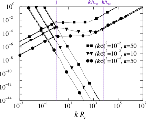
Figure 1: Plots of $\Lambda_{n}/2L_{n}^{(1)}$ (increasing curves) and $\Lambda_{n}/2L_{n}^{(2)}$ (decreasing curves) vs. $kR_{c}$ for $kd/\pi=100.5$. Dashed lines show the corresponding asymptotic expressions.

In Fig. 1 we display separately the behavior of $\Lambda_{n}/2L_{n}^{(1)}$ and $\Lambda_{n}/2L_{n}^{(2)}$, as a function of the dimensionless correlation parameter $kR_{c}$, comparing them with the analytically obtained asymptotics. The dashed lines are used to plot the asymptotics (56) and (58) for the region (55) of small-scale roughness ($kR_{c}\ll 1\lesssim k\Lambda_{n}$), and expressions (70) and (71) for the region (67) of large-scale roughness with strong correlations ($1\lesssim k\Lambda_{n}\ll kR_{c}$). As one can see, for these two regions numerical data for both lengths are quite well described by the corresponding asymptotic expressions.

The curves $\Lambda_{n}/2L_{n}^{(1)}$ clearly manifest two transition points: between the regions of small-scale and large-scale corrugations at $kR_{c}\sim 1$, and between weak and strong correlations at $kR_{c}\sim k\Lambda_{n}$. As follows from Eq. (50), the inverse value of the first attenuation length typically increases with an increase of $kR_{c}$. Specifically, within the interval of the small-scale roughness ($kR_{c}\ll 1\lesssim k\Lambda_{n}$) we have $1/L^{(1)}_{n}\propto kR_{c}$. Then, within the intermediate region of large-scale roughness with weak correlations where $1\ll kR_{c}\ll k\Lambda_{n}$, the increase of $\Lambda_{n}/2L_{n}^{(1)}$ slows down (see the curves with the parameters $(k\sigma)^{2}=10^{-2},10^{-4}$; $n=50$), or can even be replaced by the decrease for some values of the model parameters (see the curve with the parameter $(k\sigma)^{2}=10^{-2}$, $n=10$). Within these two regions that are unified under the condition $kR_{c}\ll k\Lambda_{n}$, the quantity $1/L^{(1)}_{n}$ is determined by both AS and GS mechanisms (AS+GS). Finally, for large-scale roughness and strong correlations ($1\lesssim k\Lambda_{n}\ll kR_{c}$) the value of $1/L^{(1)}_{n}$ again begins to increase linearly with $kR_{c}$. Here $1/L^{(1)}_{n}$ is associated solely with the AS mechanism because the main contribution to the asymptotic (70) is due to the diagonal term in the sum (50) .

In contrast with $1/L^{(1)}_{n}$, the inverse SGS length $1/L^{(2)}_{n}$ reveals a monotonous decrease as the parameter $kR_{c}$ increases. At small ($kR_{c}\ll 1\lesssim k\Lambda_{n}$) and extremely large ($1\lesssim k\Lambda_{n}\ll kR_{c}$) values of $kR_{c}$, this decrease obeys the law $1/L^{(2)}_{n}\propto(kR_{c})^{-3}$, due to $T(0)\sim R_{c}^{-3}$.

In Fig. 1 we can also see the crossover from the SGS to AS+GS that is characterized by the crossing point between $\Lambda_{n}/2L_{n}^{(2)}$ and $\Lambda_{n}/2L_{n}^{(1)}$. The crossing point for two curves with the parameters $(k\sigma)^{2}=10^{-4}$ and $n=50$ is very close to that for two curves with the parameters $(k\sigma)^{2}=10^{-2}$ and $n=10$. Approximately, both crossing points are

$$(kR_{c})_{cr}\sim 0.2.$$ (77)

They are located well inside the interval of small-scale roughness, and their values are in an agreement with the asymptotic expression (62). Two curves corresponding to the parameters $(k\sigma)^{2}=10^{-2}$ and $n=50$, have crossing point in the transition region $kR_{c}\sim 1$ between small- and large-scale corrugations.

In the following two Figures we display the dependence of $\Lambda_{n}/2L_{n}$ as a function of $kR_{c}$. The curves are plotted starting from the values of $kR_{c}$ for which $\Lambda_{n}/2L_{n}^{(2)}=1$, according to the first condition in (54). Taking into account the second condition restricting the maximal value of $kR_{c}$, we plot every curve within the range where $R_{c}<2L^{(1)}_{n}$. Based upon the description of the Fig. 1, the identification of each scattering mechanism dominating in the corresponding regions becomes simple. One can see that the curves in Figs. 2 and 3 experience firstly the crossover from the SGS to the AS+GS, and after, from the AS+GS to AS. We outline both transitions with the labels ‘$(kR_{c})_{cr}$’ and ‘$k\Lambda_{n}$’, respectively.

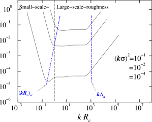
Figure 2: Plots of $\Lambda_{n}/2L_{n}$ versus $kR_{c}$ for $kd/\pi=100.5$, $n=50$, and different values of $(k\sigma)^{2}$. The dot-dashed lines labelled ‘$(kR_{c})_{cr}$’ and ‘$k\Lambda_{n}$’, indicate the transition between the regions dominated by the SGS, AS+GS and AS mechanisms (from the left to the right). The dashed line at $kR_{c}=1$ marks the transition between the regions of small-scale- and large-scale-roughness.

In Fig. 2 we show the dependence of $\Lambda_{n}/2L_{n}$ on $kR_{c}$ for three values of the parameter $(k\sigma)^{2}$ (two of them $(k\sigma)^{2}=10^{-4},10^{-2}$ correspond to those used in Fig. 1). The curve with $(k\sigma)^{2}=10^{-4}$ has the crossing point $(kR_{c})_{cr}$ of the value (77) located within the interval of small-scale roughness. The crossover reveals a small dip centered at $(kR_{c})_{cr}$. The curve obeys the asymptotic behavior $(kR_{c})^{-3}$ to the left from $(kR_{c})_{cr}$ due to the main contribution from $\Lambda_{n}/2L_{n}^{(2)}$. After, the quantity $\Lambda_{n}/2L_{n}^{(1)}$ becomes dominating in the sum (49), therefore, the curve begins to rise. Firstly, the linear dependence on $kR_{c}$ on the right deep-side (where $kR_{c}<1$) is replaced with a smoother one (for $kR_{c}>1$). Finally, for $R_{c}>\Lambda_{n}$ (strong correlations) the linear dependence restores.

The crossing points of the second and third curves with $(k\sigma)^{2}=10^{-2},10^{-1}$ have values of the order of unit, $(kR_{c})_{cr}\sim 1$. Here the total attenuation length $L_{n}$ within the whole small-scale region is formed solely by the SGS length $L_{n}^{(2)}$. In full agreement with Eq. (62) the presented curves display that the smaller the parameter $(k\sigma)^{2}$ the smaller the value of the crossing point $(kR_{c})_{cr}$.

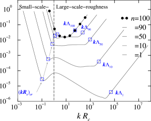
Figure 3: Plots of $\Lambda_{n}/2L_{n}$ versus $kR_{c}$ for $kd/\pi=100.5$, $(k\sigma)^{2}=10^{-2}$, and different values of the mode index $n$. The sets of square symbols labelled ‘$(kR_{c})_{cr}$’ and ‘$k\Lambda_{n}$’ play the same role as dot-dashed lines in Fig. 2.

To visualize the dependence on the mode index $n$, in Fig. 3 we plot $\Lambda_{n}/2L_{n}$ with the parameter $n$ spanning the range of the propagating modes. One can see that for the mode index $n=1$ the crossing point $(kR_{c})_{cr}\sim 0.1$, the curve with $n=10$ has $(kR_{c})_{cr}$ given by Eq. (77). For the rest of the values of $n$ the crossover occur at $(kR_{c})_{cr}\sim 1.0$. We note that the smaller the channel index $n$, the smaller the value of the crossing point $(kR_{c})_{cr}$. This fact is in full agreement with Eq. (62). The squares labelled with ‘$k\Lambda_{n}$’, show the transition points between the AS+GS and AS mechanisms (or between the weak- and strong-correlations of the surface roughness). They are $k\Lambda_{1}\approx 63500$, $k\Lambda_{10}\approx 6315$, $k\Lambda_{50}\approx 1100$, $k\Lambda_{90}\approx 310$ and $k\Lambda_{100}\approx 60$.

Finally, note that for all curves in our figures the roughness height is small, $\sigma/d\ll 1$. Furthermore, for the amplitude- and gradient-dominated scattering (to the right from the point $(kR_{c})_{cr}$ where $\Lambda_{n}/2L^{(1)}_{n}$ mainly contributes), the average corrugation slope is also small for all data, $\sigma/R_{c}\ll 1$. The roughness slope remains to be small at the crossing points too, but increases to their left with the decrease of $kR_{c}$. As a result, to the left from the crossing point where the square-gradient term $\Lambda_{n}/2L^{(2)}_{n}$ prevails, the slope reaches the values of the order one, or even larger.

VI Conclusion

In this paper we investigated the wave/electron scattering in multi-mode surface-corrugated waveguides of quasi-1D geometry. For this kind of waveguides, we have discovered a new square-gradient scattering (SGS) mechanism that is different from the previously studied ones. This mechanism arises due to specific square-gradient terms in the Hamiltonian describing the surface scattering, that are related to the roughness square-gradient power (RSGP) spectrum $T(k_{x})$. To compare with, the well known scattering mechanisms, the amplitude (AS) and the gradient (GS) ones, are both determined by the roughness-height power (RHP) spectrum $W(k_{x})$, only. Since the SGS mechanism is independent from the others, one can define two attenuation lengths, the known length $L_{n}^{(1)}$ and the SGS length $L_{n}^{(2)}$. Both contribute to the total attenuation length (or, the same, electron mean free path) $L_{n}$ according to Eq. (49).

The roughness-height $W(k_{x})$ and square-gradient $T(k_{x})$ power spectra have very different dependencies on the roughness correlation length $R_{c}$. This provides the substantially different behavior of the corresponding scattering lengths in dependence of the model parameters. Specifically, the inverse value of the first attenuation length $1/L^{(1)}_{n}$ typically increases, while the inverse value of the SGS length $1/L^{(2)}_{n}$ decreases, with an increase of the parameter $kR_{c}$. Therefore, the curves displaying these quantities intersect upon the increase of the dimensionless correlation length $kR_{c}$, and the crossover from the SGS to AS+GS occurs. To the left from the crossing point $(kR_{c})_{cr}$ the SGS length prevails over the first attenuation length, $L^{(2)}_{n}\ll L^{(1)}_{n}$. To the right from $(kR_{c})_{cr}$, the first attenuation length mainly contributes to the scattering process, $L^{(1)}_{n}\ll L^{(2)}_{n}$. If the crossing point $(kR_{c})_{cr}$ falls into the interval (55) of small-scale surface corrugations, it obeys the law (62).

As we have shown, at any fixed value of the root-mean-square roughness height $\sigma$, one can indicate the region of small values of the correlation length $R_{c}$ where the new attenuation length $L^{(2)}_{n}$ predominates over the known length $L^{(1)}_{n}$. This predominance arises in spite of the fact that $1/L^{(1)}_{n}$ is proportional to $\sigma^{2}$ while $1/L^{(2)}_{n}$ is proportional to $\sigma^{4}$.

In the large-scale roughness regime where the first attenuation length mainly contributes, $L^{(1)}_{n}\ll L^{(2)}_{n}$, one can observe two different behaviors of $1/L_{n}^{(1)}$. In the interval of weak correlations (63) the dependence of $1/L_{n}^{(1)}$ on $kR_{c}$ is quite complicated, due to the coexistence of both the AS and GS mechanisms. However in the region of strong correlations (67), because the AS stands alone, we have much simpler behavior, $1/L^{(1)}_{n}\propto kR_{c}$. It is remarkable that the SGS mechanism prevails in the widely discussed region of a small-scale boundary perturbation, $kR_{c}\ll 1$, where the surface roughness is typically described via the white-noise potential.

References

(1)
F. G. Bass, I. M. Fuks, Wave Scattering from Statistically
Rough Surfaces (Pergamon, New York, 1979).
(2)
S. M. Rytov, Yu. A. Kravtsov, and V. I. Tatarskii, Principles
of Statistical Radiophysics (Springer, Berlin, 1989).
(3)
A. R. McGurn and A. A. Maradudin, Phys. Rev. B30, 3136 (1984).
(4)
J. A. Sánchez-Gil, V. Freilikher, I. V. Yurkevich,
A. A. Maradudin, Phys. Rev. Lett. 80, 948 (1998).
(5)
J. A. Sánchez-Gil,
V. Freilikher, A. A. Maradudin, and I. V. Yurkevich, Phys. Rev. B59,
5915 (1999).
(6)
J. A. Konrady, J. Acoust. Soc. Am. 56, 1687 (1974).
(7)
Z. Tešanović, M. Jarić, S. Maekawa, Phys. Rev. Lett. 57, 2760
(1986).
(8)
N. Trivedi and N. W. Ashcroft, Phys. Rev. B38, 12298 (1988).
(9)
A. M. Bratkovsky and S. N. Rashkeev, Phys. Rev. B53, 13074 (1996).
(10)
A. E. Meyerovich and S. Stepaniants, Phys. Rev. Lett. 73, 316 (1994);
Phys. Rev. B51, 17116 (1995); Phys. Rev. B58, 13242 (1998); Phys. Rev. B60, 9129 (1999); J. Phys.: Condens. Matter 12, 5575
(2000).
(11)
G. A. Luna-Acosta, Kyungsun Na, L. E. Reichl, A. Krokhin, Phys. Rev. E53, 3271 (1996).
(12)
A. B. Isers, A. A. Puzenko, I. M. Fuks, Akust. Zh. 36, 454
(1990) [Sov. Phys. Acoust. 36, 253 (1990)]; Journal of
Electromagnetic Waves and Applications 5, 1419 (1991).
(13)
N. M. Makarov and Yu. V. Tarasov, J.Phys.: Condens. Matter 10, 1523 (1998); Phys. Rev. B64, 235306 (2001).
(14)
G. A. Luna-Acosta, J. A. Méndez-Bermúdez, F. M. Izrailev,
Phys. Rev. E 64, 036206 (2001).
(15)
A. G. Voronovich, Wave Scattering from Rough Surfaces
(Springer, Berlin, 1994).
(16) A. A. Krokhin, N. M. Makarov, V. A. Yampol’skii,
J. Phys.: Condens. Matter 3, 4621 (1991).
(17)
N. M. Makarov, A. V. Moroz, V. A. Yampol’skii, Phys. Rev. B52, 6087
(1995).
(18)
V. I. Tatarskii, Waves in Random Media 3, 127 (1993);
ibid7, 557 (1997); ibid10, 339 (2000).
(19)
A. B. Migdal, Qualitative Methods in Quantum Theory
(Benjamin, London, 1977). p. 98.
(20)
F. M. Izrailev, N. M. Makarov, M. Rendón, Phys. Rev. B72,
041403(R) (2005).