Low-energy Effective Theory for Spin Dynamics of Fluctuating Stripes

Abstract

We derive an effective Hamiltonian for spin dynamics of fluctuating smectic stripes from the t-J model in the weak coupling limit $t\gg J$. Besides the modulation of spin magnitude, the high energy hopping term would induce a low-energy anti-ferromagnetic interaction between two neighboring “blocks of spins”. Based on the effective Hamiltonian, we applied the linear spin-wave theory and found that the spin-wave velocity is almost isotropic for $\rm La_{2-x}Sr_{x}CuO_{4}$ unless the structural effect is considered. The intensity of the second harmonic mode is found to be about 10% to that of the fundamental mode.

There’s still a lot of interest on stripe physics review ; review2 . The stripe modulation was found in cuprate superconductor tranquada of the sample $\rm La_{2-x}Sr_{x}CuO_{4}$ (LSCO) in the low-temperature orthorhombic (LTO) structure. It is also consistent with the incommensurate magnetic peaks observed in the inelastic neutron scattering experiments incomm-expt , in which the peak shift from $(\pi,\pi)$ towards $(\pi,0)$ with the derivation very near to $2\pi\delta$ at doping concentration $\delta$. By partial substitution of Nd for La, the LTO lattice structure is distorted to the low-temperature tetragonal (LTT) structure crawford , in which the horizontal stripe is enhanced and the fluctuating (dynamic) stripe becomes more ordered (static).

Theoretically, by the mean-field analysis of the single-band Hubbard model hubbard , there is a possibility that the stripe phase is formed. On the other hand, by employing the Schwinger-boson mean-field theory auerbach to the t-J model, it is found that the spiral spin state incomm-th can also give the deviation from $(\pi,\pi)$ upon doping. However, it was studied by many approaches that the uniform phase is unstable towards phase separation in the range of interest ratio t/J phase-separation . One of the consequence of the phase separation is to form stripes, in order to be consistent with the neutron scattering experiments. Because of the stripe fluctuation around the hole domain, the spins across the hole domain should be anti-parallel. By considering just a small transverse fluctuation of the stripe, it was found that two neighboring spins across the hole domain feels an anti-ferromagnetic interaction of coupling $J$ zachar02 .

Although there is still controversy about the stability of stripes stability , in this paper, the fact that the fluctuating smectic stripe phase is stable is our assumption. By including the Coulomb repulsion (which is neglected in the t-J model), the holes can only phase separate at microscopic scale instead of full phase separation. In order to balance the hole kinetic energy and the Coulomb repulsion, stripes is the simplest solution among those inhomogeneous states at microscopic scale.

In the following, we are going to derive the low-energy spin dynamics from the 2D t-J model of the site-centered stripe along $y$-direction. The period of hole domain is $2R$ where $R\gg 1$ in our model.

The hopping term $H_{t}$ in the t-J model is written as

$$H_{t} = H_{t}^{\perp}+H_{t}^{\parallel}$$ (1)

$$= \sum_{\alpha}\left(H_{t}^{\perp,\alpha}+H_{t}^{\parallel,\alpha}\right)$$

where $H_{t}^{\perp}$ is the transverse fluctuation of vertical stripes, and $H_{t}^{\parallel}$ is the 1D kinetic motion along the vertical stripes. Now

$$H_{t}^{\perp,\alpha} = -t\sum_{\sigma}{\sum_{i}}^{\prime}\left(c_{i+\hat{x},\alpha,\sigma}^{\dagger}c_{i}+c_{i+2\hat{x},\alpha,\sigma}^{\dagger}c_{i+\hat{x},\alpha,\sigma}+\ldots\right.$$ (2)

$$\left.+c_{i+R\hat{x},\alpha,\sigma}^{\dagger}c_{i+(R-1)\hat{x},\alpha,\sigma}\right)+{\rm h.c.}$$

where $\alpha$ label the smectic stripes and $i_{x}$ is summed over the super-cell of period $2R$. And also

$$H_{t}^{\parallel,\alpha}=-t\sum_{\sigma}{\sum_{i}}^{\prime}c_{i+\hat{y},\alpha,\sigma}^{\dagger}c_{i,\alpha,\sigma}+{\rm h.c.}$$ (3)

In the weak coupling limit, $t\gg J$, the fluctuating stripe induces a charge-density wave along $x$-direction. There’s two almost degenerate ground states for $H_{t}^{\perp,\alpha}$, $|\psi_{\rm S}\rangle$ and $|\psi_{\rm T}\rangle$, which are expressed as

$$|\psi_{\rm S}\rangle = \frac{1}{\sqrt{2}}\left(|\psi_{1}\rangle-|\psi_{2}\rangle\right)$$ (4)

$$|\psi_{\rm T}\rangle = \frac{1}{\sqrt{2}}\left(|\psi_{1}\rangle+|\psi_{2}\rangle\right)$$ (5)

where

$$|\psi_{1}\rangle = a_{0}|\cdot\cdot\downarrow\uparrow\circ\downarrow\uparrow\cdot\cdot\rangle+a_{1}|\cdot\cdot\downarrow\uparrow\downarrow\circ\uparrow\cdot\cdot\rangle$$ (6)

$$+a_{-1}|\cdot\cdot\downarrow\circ\uparrow\downarrow\uparrow\cdot\cdot\rangle+\ldots$$

$$|\psi_{2}\rangle = a_{0}|\cdot\cdot\uparrow\downarrow\circ\uparrow\downarrow\cdot\cdot\rangle+a_{1}|\cdot\cdot\uparrow\downarrow\uparrow\circ\downarrow\cdot\cdot\rangle$$ (7)

$$+a_{-1}|\cdot\cdot\uparrow\circ\downarrow\uparrow\downarrow\cdot\cdot\rangle+\ldots$$

The basis of $|\psi_{1}\rangle$ and $|\psi_{2}\rangle$ are different by the up and down spins. The corresponding coefficients are equal. Two subspaces $\{|\psi_{1}\rangle\}$ and $\{|\psi_{2}\rangle\}$ are orthogonal to each other. By Eq.(4), which is an orthogonal transformation from $|\psi_{1}\rangle$ and $|\psi_{2}\rangle$ to $|\psi_{\rm S}\rangle$ and $|\psi_{\rm T}\rangle$, two subspaces ${\cal H}_{S}$ and ${\cal H}_{T}$ spanned by $\{|\psi_{\rm S}\rangle\}$ and $\{|\psi_{\rm T}\rangle\}$ respectively are also orthogonal to each other. Eq.(2) can be written in the following matrix form under the above basis, i.e.,

$$H_{t}^{\perp,\alpha}=(-t)\left(\begin{array}[]{ccccc}0&1&1&0&\ldots\\ 1&0&0&1&\ldots\\ 1&0&0&0&\ldots\\ 0&1&0&0&\ldots\\ \vdots&\vdots&\vdots&\vdots&\ddots\end{array}\right)\bigotimes(-t)\left(\begin{array}[]{ccccc}0&1&1&0&\ldots\\ 1&0&0&1&\ldots\\ 1&0&0&0&\ldots\\ 0&1&0&0&\ldots\\ \vdots&\vdots&\vdots&\vdots&\ddots\end{array}\right)$$ (18)

where the two identical $(2R+1)$-dimensional matrices correspond to two orthogonal subspaces spanned by $\{|\psi_{\rm S}\rangle\}$ and $\{|\psi_{\rm T}\rangle\}$. Simultaneously, the Heisenberg term in the t-J model is written in the matrix form

$$H_{J}^{\perp,\alpha}=(-\frac{3J}{4})\left(\begin{array}[]{ccccc}0&0&0&0&\ldots\\ 0&1&0&0&\ldots\\ 0&0&1&0&\ldots\\ 0&0&0&1&\ldots\\ \vdots&\vdots&\vdots&\vdots&\ddots\end{array}\right)\bigotimes(\frac{J}{4})\left(\begin{array}[]{ccccc}0&0&0&0&\ldots\\ 0&1&0&0&\ldots\\ 0&0&1&0&\ldots\\ 0&0&0&1&\ldots\\ \vdots&\vdots&\vdots&\vdots&\ddots\end{array}\right)$$ (30)

Now because two subspaces ${\cal H}_{\rm S}$ and ${\cal H}_{\rm T}$ are orthogonal to each other, the first-order correction to the ground state energy due to perturbed term $H_{J}^{\perp,\alpha}$ is

$$E_{\rm S}^{(1)} = \langle\psi_{\rm S}|H_{J}^{\perp,\alpha}|\psi_{\rm S}\rangle+O(J^{2}/t)$$ (32)

$$E_{\rm T}^{(1)} = \langle\psi_{\rm T}|H_{J}^{\perp,\alpha}|\psi_{\rm T}\rangle+O(J^{2}/t)$$ (33)

and no correction to the wavefunction since two subspaces are orthogonal. Solving the eigenproblem for $H_{t}^{\perp,\alpha}$ gives the transverse density $\rho(x)$ in $(-R,R)$ to the leading order can be obtained from the

$$\rho(x) = |\langle x|\psi_{\rm S}\rangle|^{2}=|\langle x|\psi_{\rm T}\rangle|^{2}$$ (34)

$$= \frac{\delta}{1+2/\pi}\left(1+\cos(\frac{\pi x}{2R})\right)$$

and repeat for a period $2R$. It would be convenient to define $\vec{q}_{0}=(q_{0},0)$, where $q_{0}=\pi/(2R)$. The charge-density wave induced by stripe fluctuation is

$$\rho(\vec{r})=\delta+\rho_{1}\cos(2\vec{q}_{0}\cdot\vec{r})+\rho_{2}\cos(4\vec{q}_{0}\cdot\vec{r})+\ldots$$ (35)

where $\rho_{1}=\frac{4\delta}{3(2+\pi)}$ and $\rho_{2}=-\frac{4\delta}{15(2+\pi)}$.

Eqs.(32)-(33) tells that two almost degenerate states are split by an energy difference $E_{\rm T}^{(1)}-E_{\rm S}^{(1)}$, and hence the energy difference between two “block of spins” is

$$J^{\prime}=2R\delta(E_{\rm T}^{(1)}-E_{\rm S}^{(1)})=\frac{2J\delta R^{2}}{R+1}$$ (36)

Substitution of $q_{0}=2\pi\delta$ gives $J^{\prime}=J/(2(1+4\delta))$. Notice also that the energy difference per site between anti-phase and in-phase becomes $J^{\prime}/(2R)=J\delta/(1+4\delta)$, which is almost linear in $\delta$ for $\delta\ll 1$. For $\delta=1/8$, energy difference is $J/12\simeq 130K$ (take $J=135meV$), which is consistent with the observation of the incommensurate peak up to around $100K$ incomm-expt .

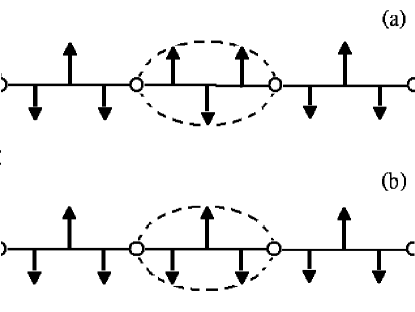
Figure 2: Illustration of the flip of a “block of spins” from (a) to (b).

There is then an effective anti-ferromagnetic coupling term between two neighboring blocks of spins. The anti-phase described by $|\psi_{\rm S}\rangle$ is of lower energy $J^{\prime}$ than the in-phase by $|\psi_{\rm T}\rangle$. Notice that it is different from the case that two neighboring spins across the hole domain interacts with an anti-ferromagnetic coupling zachar02 ; otherHam . The illustration of how to flip a block of spins is shown in Fig.2. Several mean-field type studies neglecting this low-energy interaction ogata cannot distinguish anti-phase and in-phase.

Because of no-double occupancy at every site, the spin magnitude also form a period of $2R$, in which

$$S(\vec{r}) = \frac{1}{2}(1-\rho(\vec{r}))$$ (37)

$$= S_{0}+S_{1}\cos(2\vec{q}_{0}\cdot\vec{r})+S_{2}\cos(4\vec{q}_{0}\cdot\vec{r})+\ldots$$

where $S_{0}=\frac{1}{2}(1-\delta)$, $S_{1}=-\frac{2\delta}{3(2+\pi)}$, and $S_{2}=\frac{2\delta}{15(2+\pi)}$.

Because of the anti-ferromagnetic interaction between two blocks of spins across the hole stripes, we can determine classically the $z$-component of the spin $S^{z}(\vec{r})$ which gives

$$S^{z}(\vec{r}){\rm e}^{i\vec{Q}\cdot\vec{r}}=S^{z}_{1}\sin(\vec{q}_{0}\cdot\vec{r})+S^{z}_{3}\sin(3\vec{q}_{0}\cdot\vec{r})+\ldots$$ (38)

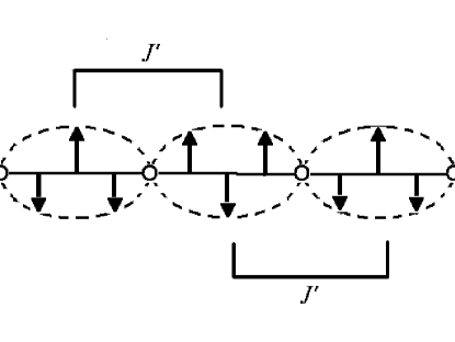
Figure 1: Schematic diagram of spin state at doping concentration $\delta=1/8$ of LSCO ($q_{0}=2\pi\delta=\pi/4$). The circles represent the zero average of spin direction. The dashed line shows the envelope of the spin component in $z$-direction. Any two neighboring “blocks of spins” feel an anti-ferromagnetic interaction of coupling $J^{\prime}$.

where $\vec{Q}=(\pi,\pi)$, $S^{z}_{1}=\frac{2}{\pi}-\frac{3\delta}{2+\pi}$, and $S^{z}_{3}=\frac{2}{3\pi}-\frac{5\delta}{3(2+\pi)}$. Notice that the components $S^{z}_{2}$, $S^{z}_{4}$, and etc vanish because of the anti-phase symmetry. Including the effect from lattice distortion gives the same result. The non-vanishing higher harmonic should have wavevector $3q_{0}$, $5q_{0}$, and etc. The schematic diagram of the classical spin state is shown in Fig.1.

Estimated up to the order of magnitude, the neutron scattering intensity is more or less proportional to

$$\int d{\vec{r}}{\rm e}^{-\vec{k}\cdot\vec{r}}\langle S^{z}(\vec{r})S^{z}(0)\rangle$$ (39)

$$\propto (S^{z}_{1})^{2}\left[\delta(\vec{k}-\vec{Q}+\vec{q}_{0})+\delta(\vec{k}-\vec{Q}-\vec{q}_{0})\right]$$

$$+(S^{z}_{3})^{2}\left[\delta(\vec{k}-\vec{Q}+3\vec{q}_{0})+\delta(\vec{k}-\vec{Q}-3\vec{q}_{0})\right]$$

$$+\ldots$$

For $\delta\ll 1$, $(S^{z}_{3}/S^{z}_{1})^{2}\simeq 1/9$. Substitute $\delta=1/8$, the ratio is 0.093. In general, the ratio of the intensities of the second harmonic ($\vec{Q}\pm 3\vec{q}_{0}$) to that of the fundamental mode ($\vec{Q}\pm\vec{q}_{0}$) is about 10%. However, the signal-to-noise ratio in current neutron scattering experiments tranquada is not high enough to observe the second harmonic peak. We expect further experiments on a larger pure single crystal measurement can verify our prediction. The first harmonic occuring at $\vec{Q}\pm 2\vec{q}_{0}$ vanishes. For LSCO, structural effect at doping concentration $\delta=1/8$ enhances the fundamental mode so that the second harmonic is even harder to be observed.

In order to obtain the low-energy properties, we apply the linear spin-wave expansion hp , i.e.,

$$\hat{S}^{z}(\vec{r}_{i}) = \pm(S(\vec{r}_{i})-b_{i}^{\dagger}b_{i})$$ (40)

$$\hat{S}^{\pm}(\vec{r}_{i}) = \sqrt{S(\vec{r}_{i})}b_{i}$$ (41)

$$\hat{S}^{\mp}(\vec{r}_{i}) = \sqrt{S(\vec{r}_{i})}b_{i}^{\dagger}$$ (42)

in which $b_{i}^{\dagger}$’s and $b_{i}$’s describe the quantum fluctuation from the classical ground state. The effective Hamiltonian for spin dynamics is

$$H_{J} = E_{0}+4J\sum_{i}S(\vec{r}_{i})b_{i}^{\dagger}b_{i}$$ (43)

$$+2J\sum_{i}\left(\sqrt{S(\vec{r}_{i})S(\vec{r}_{i+1})}b_{i}b_{i+1}+{\rm h.c.}\right)$$

In the long-wavelength limit, we replace the geometric mean $\sqrt{S(\vec{r}_{i})S(\vec{r}_{i+1})}$ by the arithmetic mean $(S(\vec{r}_{i})+S(\vec{r}_{i+1}))/2$, and then perform the Fourier transform to the variables $b_{i}^{\dagger}$ and $b_{i}$. Notice that the sites of classical spin pointing up and down are merged together in their Fourier modes. Then

$$H_{J} = E_{0}+2S_{0}J\sum_{\vec{k}}\left(2b_{\vec{k}}^{\dagger}b_{\vec{k}}+\gamma_{\vec{k}}b_{\vec{k}}b_{-\vec{k}}+\gamma_{\vec{k}}b_{-\vec{k}}^{\dagger}b_{\vec{k}}^{\dagger}\right)$$ (44)

$$+S_{1}J\sum_{\vec{k}}\left(2b_{\vec{k}+2\vec{q}_{0}}^{\dagger}b_{\vec{k}}+\gamma_{\vec{k}-2\vec{q}_{0}}b_{\vec{k}}b_{-\vec{k}+2\vec{q}_{0}}\right.$$

$$\left.+\gamma_{\vec{k}+2\vec{q}_{0}}b_{\vec{k}}b_{-\vec{k}-2\vec{q}_{0}}+{\rm h.c.}\right)$$

where $\gamma_{\vec{k}}=(\cos(k_{x})+\cos(k_{y}))/2$, and the terms involving higher harmonics are neglected. The Hamiltonian is quadratic and in principle can be straightforwardly diagonalized. Since we are only interested in the excitation spectrum around $\vec{k}=\pm 2\vec{q}_{0}$, write

$$H_{J}|_{\vec{k}\simeq\pm 2\vec{q}_{0}}=\sum_{\vec{k}\simeq 2\vec{q}_{0}}\eta_{+}^{\dagger}M_{+}\eta_{+}+\sum_{\vec{k}\simeq-2\vec{q}_{0}}\eta_{-}^{\dagger}M_{-}\eta_{-}$$ (45)

where $\eta_{\pm}=(b_{\vec{k}}\ b_{\vec{k}\mp\vec{q}}\ b_{-\vec{k}}^{\dagger}\ b_{-\vec{k}\pm\vec{q}}^{\dagger})^{T}$ and

$$M_{\pm}=J\left(\begin{array}[]{cccc}4S_{0}&2S_{1}&4S_{0}\gamma_{\vec{k}}&2S_{1}\gamma_{\vec{k}\mp 2\vec{q}}\\ 2S_{1}&4S_{0}&2S_{1}\gamma_{\vec{k}\mp 2\vec{q}}&4S_{0}\gamma_{\vec{k}\mp 2\vec{q}}\\ 4S_{0}\gamma_{\vec{k}}&2S_{1}\gamma_{\vec{k}\mp 2\vec{q}}&4S_{0}&2S_{1}\\ 2S_{1}\gamma_{\vec{k}\mp 2\vec{q}}&4S_{0}\gamma_{\vec{k}\mp 2\vec{q}}&2S_{1}&4S_{0}\end{array}\right)$$ (50)

Note that it is the bosonic version of the spin-density wave induced by charge stripes instead of the fermionic one due to Fermi surface instability gruner .

Diagonalize the Hamiltonian, we get the gapless excitation at $\vec{k}=\pm 2\vec{q}_{0}$, with the anisotropic spin-wave velocities, in which

$$\epsilon_{\vec{k}=(k_{x},0)}=4S_{0}J\left[1-\frac{S_{1}^{2}}{4S_{0}^{2}}\sec^{2}(q_{0})\right]^{\frac{1}{2}}|k_{x}\pm 2q_{0}|$$ (52)

and

$$\epsilon_{\vec{k}=(\pm 2q_{0},k_{y})}=4S_{0}J|k_{y}|$$ (53)

One can estimate the ratio of the anisotropic spin-wave velocities by the above Eqs.(52)-(53),

$$\frac{v_{x}}{v_{y}}=\left[1-\frac{S_{1}^{2}}{4S_{0}^{2}}\sec^{2}(q_{0})\right]^{\frac{1}{2}}$$ (54)

For LSCO, $q_{0}=2\pi\delta$. $v_{x}/v_{y}=1$ at $\delta=0$. At $\delta=1/8$, $v_{x}/v_{y}=0.9997$. Without the structural effect, one can safely ignore the anisotropy of spin-wave velocities. However, perturbed structural effect can be straightforwardly considered by including a term

$$-V\sum_{i}\cos(2\vec{q}_{0}\cdot\vec{r}_{i})b_{i}^{\dagger}b_{i}$$ (55)

where $V>0$ enhances the spin ordering of magnitude of period $2R$. The term behaves as a perturbed term $\delta M$ to enhance the first harmonic component $S_{1}$ of the spin magnitude.

$$\delta M=\frac{-V}{2}\left(\begin{array}[]{cc}\begin{array}[]{cc}0&1\\ 1&0\end{array}&0\\ 0&\begin{array}[]{cc}0&1\\ 1&0\end{array}\end{array}\right)$$ (62)

For perturbed $V\ll t$ where the weak coupling limit is still valid, the density profile $\rho(x)$ in Eq.(34) does not vary. Eqs.(52) and (53) are just modified by replacing $S_{1}$ by $S_{1}+V/(4J)$. At $\delta\ll 1$, we can estimate

$$\frac{v_{x}}{v_{y}}\simeq\sqrt{1-\frac{V^{2}}{4J^{2}}}$$ (63)

The anisotropy in the neutron scattering measurement is around 0.75 aeppli . Eq.(63) gives an estimate of $V\simeq 1.3J$.

If the structural effect is strong enough ($V/t\gtrsim 1$), for example, in the sample of the ordered stripe phase of $\rm La_{2}NiO_{4+\delta}$, we should go beyond the weak coupling limit such that the density profile found in Eq.(34) should also depend on $V$. The case of the ordered stripe phase will be reported elsewhere.

The author would like to thank T.K. Lee for introducing him to the stripe problem, and acknowledges numerous discussion with the colleagues at the Institute of Theoretical Physics, Chinese Academy of Sciences (ITP, CAS). The work was supported by the National Science Council of Taiwan under Grant No. NSC89-2816-M-001-0012-6, and the Visiting Scholar Program of ITP, CAS under 20C905.

References

• (1) E.W. Carlson et al., in The Physics of Conventional and Unconventional Superconductors, edited by K.H. Bennemann and J.B. Ketterson (Springer-Verlag) and references therein.
• (2) S.A. Kivelson et al., Rev. Mod. Phys. 75, 1201 (2003) and references therein.
• (3) J.M. Tranquada et al., Nature 375, 561 (1995).
• (4) S.W. Cheong et al., Phys. Rev. Lett. 67, 1791 (1991); T.E. Mason, G. Aeppli, and H.A. Mook, Phys. Rev. Lett. 68, 1414 (1992); T.R. Thurston et al., Phys. Rev. B46, 9128 (1992).
• (5) M.K. Crawford et al., Phys. Rev. B44, R7749 (1991).
• (6) D. Poilblanc and T.M. Rice, Phys. Rev. B39, R9749 (1989); J. Zaanen and O. Gunnarsson, Phys. Rev. B40, R7391 (1989).
• (7) A. Auerbach and D.P. Arovas, Phys. Rev. Lett. 61, 617 (1988).
• (8) C. Jayaprakash, H.R. Krishnamurthy, and S. Sarker, Phys. Rev. B40, R2610 (1989); C.L. Kane, P.A. Lee, T.K. Ng, B. Chakraborty, and N. Read, Phys. Rev. B41, R2653 (1990); B. Normand and P.A. Lee, Phys. Rev. B51, 15519 (1995); C.D. Batista et al., Europhys. Lett. 38, 147 (1997).
• (9) V.J. Emery, S.A. Kivelson, and H.Q. Lin, Phys. Rev. Lett. 64, 475 (1990); M. Marder, N. Papanicolaou, and G.C. Psaltakis, Phys. Rev. B41, 6920 (1990); T.I. Ivanov, Phys. Rev. B44, R12077 (1991); C.T. Shih, Y.C. Chen, and T.K. Lee, Phys. Rev. B57, 627 (1998); C.H. Cheng and T.K. Ng, Europhys. Lett. 52, 87 (2000).
• (10) O. Zachar, Phys. Rev. B65, 174411 (2002).
• (11) S.A. Kivelson and V.J. Emery, Synthetic Metals 80, 151 (1996); S.R. White and D.J. Scalapino, Phys. Rev. Lett. 80, 1272 (1998); C.S. Hellberg and E. Manousakis, Phys. Rev. Lett. 83, 132 (1999); N.G. Zhang and C.L. Henley, Phys. Rev. B68, 014506 (2003).
• (12) Ref.[10] considered the hole stripes fluctuation inside the three-leg ladder, and it is somehow equivalent to introducing the structural effect implicitly.
• (13) For example, A. Himeda, T. Kato, and M. Ogata, Phys. Rev. Lett. 88, 117001 (2002). The energy difference between the anti-phase and in-phase spin domains at $\delta=1/8$ in their study is about $0.002t=8K$ (take $t=0.4eV$), while the incommensurate peaks can still be observed up to around $100K$.
• (14) T. Holstein and H. Primakoff, Phys. Rev. 58, 1098 (1940).
• (15) G. Grüner, Rev. Mod. Phys. 66, 1 (1994).
• (16) G. Aeppli et al., Phys. Rev. Lett. 62, 2052 (1989).
Refer to caption