Also at ]Institute of Industrial Science, University of Tokyo, 4-6-1 Komaba, Meguro-ku, Tokyo 153-8505, Japan

A mesoscopic Resonating Valence Bond system on a triple dot

Abstract

We theoretically introduce a mesoscopic pendulum from a triple dot. The pendulum is fastened through a singly-occupied dot (spin qubit). Two other strongly capacitively coupled islands form a double-dot charge qubit with one electron in excess oscillating between the two low-energy charge states $(1,0)$ and $(0,1)$. The triple dot is placed between two superconducting leads. Under realistic conditions, the main proximity effect stems from the injection of resonating singlet (valence) bonds on the triple dot. This gives rise to a Josephson current that is charge- and spin-dependent and, as a consequence, exhibits a distinct resonance as a function of the superconducting phase difference.

By analogy with quantum optics, the production of entangled states in condensed matter devices have inherently emerged as a mainstream in nanoelectronicsNielson . Entanglement between electrons, besides checking fundamental quantum properties such as non-locality, could be exploited for building logical gates and quantum communication devices. The realization of electron entangled states might result from strong interactions in nanoscopic systems. Mostly, this offers a room to treat the spin in a quantum dot as a qubitLoss with generally a quite long decoherence timeKouw ; Marcus . Spin entanglement scenarios have been envisioned in such a frameworkEnt . Theoretical research on the possibility to control and detect the spin of electrons through their charges has also blossomed recentlyLesovik ; Buttiker ; Saraga . Let us recall that the direct coupling of two quantum dots by a tunnel junction might be used to create entanglement between spinsLoss and such spin correlations might be observed in transport experimentsLoss1 . Another mechanism to induce spin correlations would consist to place a double quantum dot away from resonance in a vertical configuration between two superconducting (SC) leadsChoi . We go beyond and (theoretically) explore other entanglement mechanisms based on triple dot devices and more precisely on the prolific proximity between a spin and a double-dot charge qubit. We consider the idea to realize singlets resonating between equivalent low-energy configurations on a triple dot by placing the latter between two SC electrodes. This can be viewed as a mesoscopic Resonating Valence Bond (RVB) systemAnderson resulting in a Josephson current with a distinct resonant-like profile as a function of the superconducting phase difference.

The pillar of this mesoscopic RVB system is what we refer to as the mesoscopic pendulum. We take two strongly capacitively coupled quantum dots (say, dots 1 and 3 of Fig. 1) that form a charge qubit; only one electron in excess is permitted on dots 1 and 3 which thus embodies the weight of the pendulum. The pendulum is fixed through the dot 2 which is singly-occupied and off resonance (spin qubit).

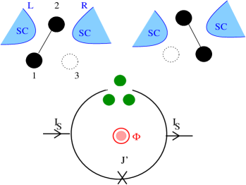
Figure 1: (Color online) The pendulum with resonating singlet bonds under consideration: The dots 1 and 3 are strongly capacitively coupled and form a two-level system characterized by the degenerate orbital states $(1,0)$ or $(0,1)$. Dot 2 is singly occupied and the direct tunnel coupling between dots 1 and 2 (or 2 and 3) is negligible. The spin entanglement induced by the SC leads between dot 2 and, say, dot 1 (or dot 3), embodies the rod of the pendulum. The singlets can also resonate through the direct tunnel coupling ${\cal T}^{\prime}$ between dots 1 and 3. Consequences in a SQUID geometry are properly analyzed.

Then, we place the quantum pendulum between two SC leads. The rod of the pendulum in Fig. 1 represents the emergence of spin entanglement between dot 2 and, say, dot 1, induced by the proximity from the SC leads. Through the tunnel coupling ${\cal T}^{\prime}$ between dots 1 and 3 and the closeness of the SC leads, hence the singlet bonds will resonate on the triple dot.

Model.— Assuming that the capacitive coupling between dot 1 (dot 3) and dot 2 is negligible (that is quite legitimate for the situation of Fig. 1), the general charging energy for the dots 1 and 3 takes the standard formWiel $E_{n_{1}n_{3}}=E_{c1}(n_{g1}-n_{1})^{2}+E_{c3}(n_{g3}-n_{3})^{2}+E_{c13}(n_{g1}-n_{1})(n_{g3}-n_{3})$, where we have introduced the charging energies $E_{c1,3}=e^{2}C_{\Sigma 3,1}/[2(C_{\Sigma 1}C_{\Sigma 3}-C_{13}^{2})]$, $E_{c13}=e^{2}C_{13}/(C_{\Sigma 1}C_{\Sigma 3}-C_{13}^{2})$. Here, $n_{g1,3}=C_{g1,3}V_{g1,3}/e$ are the mean numbers of holes on the gates — coupled to dots 1 and 3 through the capacitances $C_{g1,3}$ — being used to change the numbers of electrons $n_{1}$ and $n_{3}$ on dots 1 and 3 through the gate voltages $V_{g1,3}$, $C_{13}$ stands for the capacitive coupling between dots 1 and 3, and $C_{\Sigma 1,3}=C_{g1,3}+C_{13}$. Of interest to us is the strong inter-dot capacitive limit $C_{13}\sim C_{g1,3}$ with $n_{g1}\sim n_{g3}\sim 1/2$ such that $E_{01}\sim E_{10}\ll(E_{00},E_{11})\ll(E_{20},E_{02})$. The low energy physics can thus be studied within the restricted Hilbert space in which only the $(n_{1},n_{3})=(0,1)$ and $(1,0)$ states are allowed for the dots 1 and 3. The manipulation of a single charge in a double dot is now well accessible experimentallyHayashi ; Dicarlo ; Petta ; Jeong . A similar regime can be reached with SC dotsPashkin ; Levy . We assume that the dots 1 and 3 form a nonlocal charge qubit (with only one electron in excess) and thus we can resort to the projecting operators $\hat{P}_{01}$ and $\hat{P}_{10}$ to project on the $(0,1)$ and $(1,0)$ states respectivelyMeirong . Below, we refer to ${\cal H}_{13}$ as the charging Hamiltonian for dots 1 and 3 related to $E_{n_{1}n_{3}}$.

The dot 2 contains one electron in excess at the energy $\epsilon_{2}=-\epsilon$ with $\epsilon>0$ (spin qubit) and is subject to a strong on-site Coulomb repulsion $U$ which is typically the charging energy on dot 2, leading to the Hamiltonian

$${\cal H}_{2}=\epsilon_{2}\sum_{\sigma}d^{\dagger}_{2\sigma}d_{2\sigma}+Ud^{\dagger}_{2\uparrow}d_{2\uparrow}d^{\dagger}_{2\downarrow}d_{2\downarrow}.$$ (1)

The SC leads are described by the BCS Hamiltonian

$${\cal H}_{SC}=\sum_{j=L,R}\int_{\Omega_{j}}\frac{d{\bf r}}{\Omega_{j}}\sum_{\sigma=\uparrow,\downarrow}\Psi^{\dagger}_{\sigma}({\bf r})x({\bf r})\Psi_{\sigma}({\bf r})$$ (2)

$$+\Delta_{j}({\bf r})\Psi^{\dagger}_{\uparrow}({\bf r})\Psi^{\dagger}_{\downarrow}({\bf r})+\hbox{H.c.},$$

where $\Omega_{j}$ is the volume of lead $j$, $x({\bf r})=(-i\hbar\nabla+\frac{e}{c}{\bf A})^{2}/(2m)-\mu$, and $\Delta_{j}({\bf r})=\Delta_{j}e^{-i\phi_{j}({\bf r})}$ is the pair potential. For simplicity, we assume identical leads with the same chemical potentials $\Delta\mu=0$ and $\Delta_{L}=\Delta_{R}=\Delta$. Finally, the relevant tunneling Hamiltonians take the form

$${\cal H}_{\cal T} = \sum_{j=L,R;\sigma=\uparrow,\downarrow}{\cal T}_{2}e^{i\phi({\bf r}_{j}-{\bf r}_{2})}\Psi^{\dagger}_{\sigma}({\bf r}_{j})d_{2\sigma}+\hbox{H.c.}$$

$$+ \sum_{\sigma=\uparrow,\downarrow}{\cal T}_{1}e^{i\phi({\bf r}_{L}-{\bf r}_{1})}\Psi^{\dagger}_{\sigma}({\bf r}_{L})d_{\sigma}\hat{P}_{10}+\hbox{H.c.}$$

$$+ \sum_{\sigma=\uparrow,\downarrow}{\cal T}_{3}e^{i\phi({\bf r}_{R}-{\bf r}_{3})}\Psi^{\dagger}_{\sigma}({\bf r}_{R})d_{\sigma}\hat{P}_{01}+\hbox{H.c.}.$$

$${\cal H}_{{\cal T}^{\prime}} = |{\cal T}^{\prime}|e^{i\lambda}e^{i\phi({\bf r}_{3}-{\bf r}_{1})}\hat{Q}^{+}+\hbox{H.c.}.$$

We have introduced the Aharonov-Bohm phase $\phi({\bf r}_{n}-{\bf r}_{m})=-\frac{\pi}{\Phi_{0}}\int_{{\bf r}_{m}}^{{\bf r}_{n}}d{\bf l}\cdot{\bf A}$ and $\Phi_{0}=hc/2e$ is the SC flux quantum. Here, the symbols ${\bf r}_{1}$, ${\bf r}_{2}$, and ${\bf r}_{3}$ refer to the positions of the dots 1,2, and 3, respectively whereas ${\bf r}_{L}$ and ${\bf r}_{R}$ embody the coordinates in the SC leads L and R. Note that in the present setup, an electron on dot 1 can either tunnel into the SC lead $L$ or still onto dot $3$ via ${\cal T}^{\prime}=|{\cal T}^{\prime}|\exp(i\lambda)$. Similarly, an electron on dot 3 can either tunnel into the SC lead $R$ or on dot 1. The tunnel coupling between dot 2 and, say, dot 1 (or dot 3), is negligible. Since there is a single electron in excess delocalized between dots 1 and 3 we find it convenient to introduce a unique electron annihilation operator $d_{\sigma}$ such that $\sum_{\sigma}d^{\dagger}_{\sigma}d_{\sigma}=1$, $d_{\sigma}\hat{P}_{10}=d_{1\sigma}\hat{P}_{10}$, and $d_{\sigma}\hat{P}_{01}=d_{3\sigma}\hat{P}_{01}$, with $d_{1\sigma}$ $(d_{3\sigma})$ annihilating explicitly an electron on dot $1$ $(3)$. Along the lines of Refs. Meirong, ; Borda, , we have also exploited the double-dot charge qubit notations for ${\cal H}_{{\cal T}^{\prime}}$. The raising operator $\hat{Q}^{+}$ — acting exclusively on the state $|n_{1}n_{3}\rangle$ — ensures that each time an electron travels from dot 1 to dot 3 this causes a flip $(1,0)\rightarrow(0,1)$ that means $\hat{Q}^{+}|10\rangle=|01\rangle$, $\hat{Q}^{-}|01\rangle=|10\rangle$, $\hat{Q}_{z}=(\hat{P}_{01}-\hat{P}_{10})/2$, and $\hat{Q}^{+}|01\rangle=0$. Bear in mind that, for ${\cal H}_{\cal T}=0$, the double-dot charge qubit is embodied by the ground-state wave functionWiel $|\Psi_{Q}\rangle=\sqrt{P_{10}}|10\rangle-\sqrt{{P}_{01}}e^{-i\phi({\bf r}_{1}-{\bf r}_{3})+i\lambda}|01\rangle$ with $P_{10}=\langle\Psi_{Q}|\hat{P}_{10}|\Psi_{Q}\rangle=\langle\hat{P}_{10}\rangle$ and $P_{01}=\langle\Psi_{Q}|\hat{P}_{01}|\Psi_{Q}\rangle$ satisfying $\langle\Psi_{Q}|{\cal H}_{\cal T^{\prime}}|\Psi_{Q}\rangle=-|{\cal T^{\prime}}|$ when $P_{01}=P_{10}=1/2$. Below, we consider ${\cal T}_{1}={\cal T}_{2}={\cal T}_{3}={\cal T}$. The total Hamiltonian reads ${\cal H}={\cal H}_{0}+{\cal H}_{\cal T}+{\cal H}_{{\cal T}^{\prime}}$ with ${\cal H}_{0}={\cal H}_{13}+{\cal H}_{2}+{\cal H}_{SC}$.

Charge qubit at resonance.— Let us start with $E_{01}=E_{10}=E_{Q}$. The low-energy subspace is made of one localized electron on dot 2 and one electron delocalized on dots 1 and 3. Now we derive an effective Hamiltonian ${\cal H}^{eff}$ respecting this reduced Hilbert space. The low-energy states are well separated by the superconducting gap $\Delta$ as well as the Coulomb repulsions $U$ and $E_{20}$ or $E_{02}$. We assume that dot 2 is small enough such as $U-\epsilon\gg\epsilon$ to hinder a double occupancy on dot 2; by construction $(E_{20},E_{02})\gg(E_{11},E_{00})$. We introduce $P$ the projection operator on the lowest-energy subspace and $K=(1-P)$ the projection operator on excited states:

$${\cal H}^{eff}=P{\cal H}P+P{\cal H}K\frac{1}{E-K{\cal H}K}K{\cal H}P.$$ (4)

An expansion in ${\cal H}_{\cal T}$ can be performed and we identify $E$ with $E_{Q}-\epsilon$, i.e., with the ground-state energy associated to ${\cal H}_{0}$. We envision the limit where $\epsilon/\Delta\ll 1$, nevertheless $\epsilon>0$ to ensure a trapped electron on dot 2, and $E_{00}-E_{Q}\ll\Delta$ such that we can disregard individual qubit (and Kondo) contributions. This realm can be achieved experimentally by adjusting the gate voltages of the dot 2 and of the double-dot charge qubit. Temperatures are less than $\epsilon$ and $(E_{00}-E_{Q})$ (close to zero).

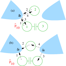
Figure 2: (Color online) Main nonlocal Andreev mechanisms when the electron on the double-dot charge qubit is initially on dot 1 and $E_{10}\sim E_{01}=E_{Q}$. The numbered arrows indicate the direction and the order of the electron transfers. Since $\epsilon\ll\Delta$ and $E_{00}-E_{Q}\ll\Delta$, we ignore individual contributionsChoi from dot 2 giving a $\pi$-junctionGlazman and from the charge qubitBorda .

The main proximity effects with the SC leads containing $\hat{P}_{10}$ are the nonlocal Andreev tunneling processes of Figs. (2a) and (2b) resulting in a nonlocal spin-entangled electron state; the second-order contribution gives a constant. Assuming $E_{00}\ll E_{11}$ we omit the superconducting cotunneling involving the transfer of the electron on dot 2 to dot 3 through the SC electrode R (involving the $(1,1)$ charge state) and then the transfer of the electron on dot 1 to dot 2 through the SC lead L; however, this would only renormalize $|{\cal T}^{\prime}|$. Other (parasitic) SC cotunneling terms can be completely ignored through the prerequisite $U-\epsilon\gg\epsilon$ (and $(E_{20},E_{02})\gg E_{00}$). Below, we build explicitly the effective ${\cal H}^{eff}$ in terms of the phase $\varphi=\phi_{L}({\bf r}_{L})-\phi_{R}({\bf r}_{R})-\frac{\pi}{\Phi_{0}}\int_{{\bf r}_{R}}^{{\bf r}_{L}}(d{\bf l}_{13}+d{\bf l}_{2})\cdot{\bf A}$ (notice that the integration from ${\bf r}_{R}$ to ${\bf r}_{L}$ runs via dot 2 or dots 1 and 3):

$${\cal H}^{eff} = {\cal H}_{0}+{\cal H}_{{\cal T}^{\prime}}+J\left({\bf S}_{2}\cdot{\bf S}-\frac{1}{4}\right)\left(\hat{P}_{10}+\hat{P}_{01}\right)$$

$$+ Je^{i\varphi-i\phi({\bf r}_{1}-{\bf r}_{3})}\left({\bf S}_{2}\cdot{\bf S}-\frac{1}{4}\right)\hat{Q}^{+}\hat{P}_{10}$$

$$+ Je^{-i\varphi+i\phi({\bf r}_{1}-{\bf r}_{3})}\left({\bf S}_{2}\cdot{\bf S}-\frac{1}{4}\right)\hat{Q}^{-}\hat{P}_{01}.$$

Remember that $\phi({\bf r}_{1}-{\bf r}_{3})=-\frac{\pi}{\Phi_{0}}\int_{{\bf r}_{3}}^{{\bf r}_{1}}d{\bf l}_{13}\cdot{\bf A}$ depicts the Aharonov-Bohm phase accumulated to go from dot 3 to dot 1, $\varphi-\phi({\bf r}_{1}-{\bf r}_{3})$ does not depend on $\lambda$, and by construction $J>0$. Here, ${\bf S}=\sum_{\alpha\beta}d^{\dagger}_{\alpha}\frac{{\bf\sigma}_{\alpha\beta}}{2}d_{\beta}$ embodies the spin of the delocalized electron on dots 1 and 3. An entanglement occurs between the spin on dot 2 and the spin ${\bf S}$ of the delocalized qubit. The process of Fig. (2b) enables the singlets to resonate via ${\bf S}_{2}\cdot{\bf S}|10\rangle\rightarrow{\bf S}_{2}\cdot{\bf S}\hat{Q}^{+}\hat{P}_{10}|10\rangle={\bf S}_{2}\cdot{\bf S}|01\rangle$. Since ${\cal H}_{\cal T^{\prime}}$ does not involve spin degrees of freedom this does not affect the spin entanglement. On the contrary, through a flip $\hat{P}_{10}\rightarrow\hat{P}_{01}$ this also stimulates the resonance of the singlets. The antiferromagnetic exchange coupling reads

$$J(\delta r)=\frac{2\Gamma^{2}}{\epsilon+E_{00}-E_{Q}}\left(\frac{\sin(k_{F}\delta r)}{k_{F}\delta r}\right)^{2}\exp(-2\delta r/\pi\xi),$$ (6)

where $\Gamma=\pi|{\cal T}|^{2}{\cal N}(0)$ with ${\cal N}(0)$ being the normal state density of states per spin of the leads at the Fermi energy ${\epsilon}_{F}>\Delta$ and ${\bf k}_{F}$ $(k_{F}=|{\bf k}_{F}|)$ being the Fermi momentum. Note that the lowest-order expansion (4) in ${\cal H}_{\cal T}$ is valid in the limit where $\Gamma\ll\epsilon+E_{00}-E_{Q}$. Here, $\xi=v_{F}/(\pi\Delta)$ with $v_{F}$ the Fermi velocity represents the coherence length of the SC leads. Remember that $\delta r$ denotes the typical distance between two injected spin-entangled electrons in a given SC lead in the case where one electron stems from dot 2 and the other from, say, dot 1. Thus, to have $J(\delta r)$ non-zero, $\delta r$ should not exceed the SC coherence length. For conventional s-wave superconductors the coherence length $\xi$ is on the order of

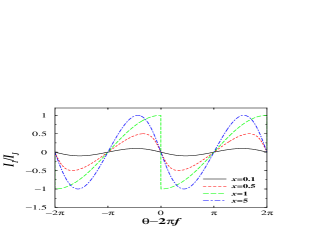
Figure 3: (Color online) $I_{1}/I_{J}$ versus $\theta-2\pi f$ for different values of $x=|{\cal T}^{\prime}|/J$. When ${\cal T^{\prime}}\sim 0$, $E^{eff}$ does not depend on $\phi_{R}-\phi_{L}$ resulting in $I_{1}=0$. When $|{\cal T^{\prime}}|\gg J$, the sinus-like profile is reminiscent of the double dot caseChoi . For $|{\cal T^{\prime}}|=J$, when the interference $|\langle\Psi_{J}|\Psi_{Q}\rangle|$ is fully destructive ($|\langle\Psi_{J}|\Psi_{Q}\rangle|\rightarrow 0$) and $\sin(\theta-2\pi f)$ changes sign, an abrupt jump in $I_{1}$ occurs.

micrometers and thus this poses not severe experimental restrictions. The suppression of $J(\delta r)$ is only polynomial $\propto(1/k_{F}\delta r)^{2}$. Exploiting parameters for a two-dimensional electron gas (InAs or GaAs) coupled to a superconductor (Al or Nb) leads to $J\sim 0.05-0.5$KChoi . The ground-state energy (the lowest eigenenergy) for a singlet state on the triple dot with $\langle{\bf S}_{2}{\bf S}-\frac{1}{4}\rangle=-1$ then can be evaluated in the charge subspace $(|10\rangle,|01\rangle)$:

$$E^{eff}=E_{Q}-J-\epsilon-\left(J^{2}+|{\cal T}^{\prime}|^{2}-2J|{\cal T}^{\prime}|\cos(\varphi-\lambda)\right)^{1/2}.$$ (7)

We emphasize that the mesoscopic RVB system might be detectable through the SQUID-ring setup in Fig. 1; note that an excited triplet state on the triple dot leading to $\langle{\bf S}_{2}{\bf S}-\frac{1}{4}\rangle=0$ does not contribute to the supercurrent.

SQUID analysis.— The Josephson current through the junction reads $I_{1}=(2\pi c/\Phi_{0})\partial E^{eff}/\partial(\phi_{R}-\phi_{L})$. When a Cooper pair accomplishes a roundtrip along the SQUID loop, we get the phase sum rule $2\pi f=2\pi\Phi/\Phi_{0}=\theta+\varphi-\lambda$ where $\Phi$ is the flux threading the SQUID loop, $\varphi-\lambda$ is the total (gauge-invariant) phase difference accross the triple dot, and $\theta\neq 0$ is the gauge-invariant phase difference accross the auxiliary junction $(J^{\prime})$. Thus

$$I_{1}=-I_{J}\frac{|{\cal T^{\prime}}|\sin(\theta-2\pi f)}{\left(J^{2}+|{\cal T}^{\prime}|^{2}-2J|{\cal T}^{\prime}|\cos(\theta-2\pi f)\right)^{1/2}},$$ (8)

with the critical current $I_{J}=2eJ/\hbar\sim 5-50nA$. Note, in Fig. 1, $I_{S}=I_{1}+(2eJ^{\prime}/\hbar)\sin\theta$. Note also that $I_{1}$ in Eq. (8) shows a resonance which is a distinct feature of this mesoscopic RVB setup. Two limiting cases can be distinguished. When $|{\cal T}^{\prime}|\gg J$, the dots 1 and 3 form a unique effective grain. Here $I_{1}=-I_{J}\sin(\theta-2\pi f)$ resembles the supercurrent through a double dot in a vertical configurationChoi ; the extra minus sign results from the interplay between ${\cal H}_{{\cal T}^{\prime}}$ and the Andreev process of Fig. 2b. When ${\cal T}^{\prime}=0$, we infer that $I_{1}=0$ (up to negligible contributions from paths involving only dot 2Choi ). The dots 1 and 3 are still coupled through the Andreev process of Fig. (2b) that is described by the phase $\varphi-\phi({\bf r}_{1}-{\bf r}_{3})$. Thus, projecting Eq. (5) on the singlet state of the triple dot, the charge qubit is embodied by the ground-state wave function $|\Psi_{J}\rangle=\sqrt{P_{10}}|10\rangle+\sqrt{P_{01}}e^{i(\varphi-\phi({\bf r}_{1}-{\bf r}_{3}))}|01\rangle$ with $P_{10}=P_{01}=1/2$ at resonance. This gives $E^{eff}=\langle\Psi_{J}|H^{eff}|\Psi_{J}\rangle=E_{Q}-\epsilon-2J$. The charge qubit seeks to react by minimizing the energy independently of $\phi_{R}-\phi_{L}$.

Now, let us discuss the highly-resonating situation $|{\cal T}^{\prime}|=J$. Owing to $|\langle\Psi_{J}|\Psi_{Q}\rangle|^{2}=[1-\cos(\theta-2\pi f)]/2$, $\frac{I_{1}}{I_{J}}\approx-\sin(\theta-2\pi f)/(2|\langle\Psi_{J}|\Psi_{Q}\rangle|).$ For half-integer values of $f$ if $\theta$ is around zero, we recover a conventional sinus-like behavior $I_{1}=-I_{J}|{\cal T^{\prime}}|\sin(\theta-2\pi f)/(J+|{\cal T^{\prime}}|)\sim-I_{J}\sin(\theta-2\pi f)/2$. On the other hand, for $(\theta-2\pi f)\approx 0$ or integer values of $f$, we observe that $|\langle\Psi_{J}|\Psi_{Q}\rangle|\rightarrow 0$. Such a destructive “interference” effect between ${\cal H}_{{\cal T}^{\prime}}$ and the Andreev process of Fig. (2b) results in a marked jump in the supercurrent (Fig. 3). The denominator in Eq. (8) becomes zero whereas $\sin(\theta-2\pi f)$ changes sign. Jumps in $I_{1}$ only emerge in the highly-resonating regime $|{\cal T}^{\prime}|=J$ for the singlets and around $\theta-2\pi f=2\pi n$ ($n$ is an integer) where $I_{1}=-I_{J}sgn(\theta-2\pi f-2\pi n)$. For $\theta$ close to zero and $\Phi=0$, the supercurrent yields $|I_{1}|=I_{J}$; this stands for a distinct hallmark of this triple dot setup.

Charge qubit off resonance.— For a finite energy splitting $\delta E=E_{01}-E_{10}>0$, we must add the extra term $\delta E\hat{Q}_{z}=\delta E(\hat{P}_{01}-\hat{P}_{10})/2$ in ${\cal H}^{eff}$. When $\delta E\ll(|{\cal T}^{\prime}|,J)$ we expect that this does not affect much the preceding results. On the contrary, for $\delta E\gg(|{\cal T}^{\prime}|,J)$, to minimize energy the double-dot charge qubit will satisfy $P_{10}=1$ and $P_{01}=0$. Here, $|01\rangle$ becomes a virtual (excited) state and this will obviously hinder the resonance of the singlets on the triple dot. For instance, $P{\cal H}_{{\cal T}^{\prime}}P=0$ and

$${\cal H}^{eff} = {\cal H}_{0}+\delta E\hat{Q}_{z}+J\left({\bf S}_{2}\cdot{\bf S}-\frac{1}{4}\right)\hat{P}_{10}$$

$$- \frac{2|{\cal T}^{\prime}|}{\delta E}J\cos(\varphi-\lambda)\left({\bf S}_{2}\cdot{\bf S}-\frac{1}{4}\right)\hat{Q}^{-}\hat{Q}^{+}\hat{P}_{10}.$$

Since $\hat{Q}^{-}\hat{Q}^{+}\hat{P}_{10}=\hat{P}_{10}$ we check that the spin entanglement now always involves the spin of the dot 1. We had to go one step further in the expansion of the effective Hamiltonian in Eq. (4) by including a final tunnel event from dot 3 to dot 1. There is another allowed process where the electron on dot 1 first tunnels onto dot 3, hence the electrons from dots 2 and 3 leave into the SC electrode R. Finally, a Cooper pair leaves the SC lead L allowing to return to the state $|10\rangle$. The singlet contribution to $I_{1}$ reads $-I_{J}(2|{\cal T}^{\prime}|/\delta E)\sin(\theta-2\pi f)$. By analogy to the double-dotChoi , the supercurrent profile is sinus-like.

Conclusion.— We have theoretically introduced a triple dot that is a mounting between a double-dot charge qubit and a spin qubit. By placing the triple dot between two SC electrodes, a spin entanglement can emerge between the spin qubit and the spin of the delocalized electron on the double-dot charge qubit. When the charge qubit is at resonance, the singlets propagate freely on the triple dot owing to the equivalence between the charge states $(1,0)$ and $(0,1)$ resulting in a mesoscopic RVB system and clear predictions. When the resonance of the singlets is maximized, i.e., for $|{\cal T^{\prime}}|=J$, we predict jumps in the supercurrent occurring for integer values of $f=\Phi/\Phi_{0}$ if $\theta$ is around zero. To reach $|{\cal T}^{\prime}|=J$, one could tune the tunnel coupling beween dots 1 and 3 similar to Refs. Petta, ; Jeong, . Since supercurrents can flow through a high-mobility AlGaAs/GaAs two-dimensional electron gasMarsh , our proposal might be realized in the future.

Acknowledgments.— We acknowledge M.-R. Li and E. Sukhorukov for discussions. This work is supported by CIAR, FQRNT, and NSERC (KLH), by the Swiss NSF, NCCR Nanoscience, EU Spintronics, and DARPA (DL), and by the University of Tokyo, JST, and NTT (PR).

References

(1)
M. A. Nielsen and I. L. Chuang, Quantum Computation & Quantum Information (Cambridge University press, 2000).
(2)
D. Loss and D. P. DiVincenzo, Phys. Rev. A 57, 120 (1998).
(3)
J. M. Elzerman, R. Hanson, L. H. W. van Beveren, B. Witkamp, L. M. K. Vandersypen and L. P. Kouwenhoven, Nature 430, 431 (2004).
(4)
A. C. Johnson, J. R. Petta, J. M. Taylor, A. Yacoby, M. D. Lukin, C. M. Marcus, M. P. Hanson, A. C. Gossard, Nature 435, 925 (2005).
(5)
G. Burkard, D. Loss, D. P. DiVincenzo, Phys. Rev. B 59, 2070 (1999); P. Recher, E. V. Sukhorukov, and D. Loss, ibid.63, 165314 (2001); J. W. D. Oliver, F. Yamaguchi, and Y. Yamamoto, Phys. Rev. Lett. 88, 037901 (2002).
(6)
G. B. Lesovik et al., Eur. Phys. J. B 24, 287 (2001).
(7)
P. Samuelsson et al., Phys. Rev. B 70, 115330 (2004).
(8)
D. S. Saraga and D. Loss, Phys. Rev. Lett. 90, 166803 (2003).
(9)
D. Loss and E. V. Sukhorukov, Phys. Rev. Lett. 84 1035 (2000).
(10)
M.-S. Choi, C. Bruder, and D. Loss, Phys. Rev. B 62, 13569 (2000).
(11)
P. W. Anderson, Science 235, 1196 (1987).
(12)
W. G. van der Wiel et al.,
Rev. Mod. Phys. 75 No. 1, 1-22 (2003).
(13)
T. Hayashi et al., Phys. Rev. Lett. 91, 226804 (2003).
(14)
L. DiCarlo et al., Phys. Rev. Lett. 92, 226801 (2004).
(15)
J. R. Petta et al., Phys. Rev. Lett. 93, 186802 (2004).
(16)
M. Pioro-Ladrière et al., Phys. Rev. B 72, 125307 (2005).
(17)
Y. Pashkin et al., Nature 421, 823 (2003).
(18)
E. Bibow et al., Phys. Rev. Lett. 88, 017003 (2002).
(19) M.-R. Li and K. Le Hur, Phys. Rev. Lett. 93, 176802 (2004).
(20)
L. Borda et al., Phys. Rev. Lett. 90, 026602 (2003).
(21)
L. I. Glazman and K. A. Matveev, JETP Lett. 49, 659 (1989); B. I. Spivak, S. A. Kivelson, Phys. Rev. B 43, 3740 (1991).
(22)
A.M. Marsh et al., Phys. Rev. B 50, R8118 (1994).