Mott transitions in two-orbital Hubbard systems

Abstract

We investigate the Mott transitions in two-orbital Hubbard systems. Applying the dynamical mean field theory and the self-energy functional approach, we discuss the stability of itinerant quasi-particle states in each band. It is shown that separate Mott transitions occur at different Coulomb interaction strengths in general. On the other hand, if some special conditions are satisfied for the interactions, spin and orbital fluctuations are equally enhanced at low temperatures, resulting in a single Mott transition. The phase diagrams are obtained at zero and finite temperatures. We also address the effect of the hybridization between two orbitals, which induces the Kondo-like heavy fermion states in the intermediate orbital-selective Mott phase.

1 Introduction

Strongly correlated electron systems with some orbitals have been investigated extensively.[1, 2] In particular, substantial progress in the theoretical understanding of the Mott transition in multiorbital systems has been made by dynamical mean-field theory (DMFT) [3, 7, 6, 4, 5] calculations. [21, 30, 34, 22, 23, 24, 25, 26, 27, 28, 29, 31, 33, 36, 32, 35, 16, 38, 37, 8, 14, 15, 17, 18, 19, 10, 11, 12, 20, 13, 9, 39, 40] Among them, the orbital-selective Mott transition (OSMT)[41] has been one of the most active topics in this context. A typical material is the single-layer isovalent ruthenate alloy Ca_2-xSr_xRuO₄[44, 42, 43]. The end-member Sr₂RuO₄ is a well-known unconventional superconductor [45, 46], while Ca₂RuO₄ is a Mott-insulating $S=1$ antiferromagnet [47, 48, 49]. The relevant $4d$-orbitals belong to the $t_{2g}$-subshell. The planar structure prevents the hybridization between orbitals which have even ($d_{xy}$) and odd parity ($d_{yz},d_{zx}$) under the reflection $z\to-z$. The complex evolution between these different end-members has stimulated theoretical investigations [50, 51, 52, 53], and among others to the proposal of the OSMT: some of the $d$-orbitals fall in localized states, while the others provide itinerant electrons. The OSMT scenario could explain the experimental observation of a localized spin $S=1/2$ in the metallic system at $x\sim 0.5$ in Ca_2-xSr_xRuO₄, which is difficult to obtain from the entirely itinerant description [41, 52, 54]. Another example of the OSMT is the compound $\rm La_{n+1}Ni_{n}O_{3n+1}$.[55] It is reported that the OSMT occurs in the $e_{g}$-subshell at the critical temperature $T_{c}\sim 550K$, below which the conduction of electrons in the $3d_{x^{2}-y^{2}}$ orbital is disturbed by the Hund coupling with the localized electrons in the $3d_{3z^{2}-r^{2}}$ orbital.[56] These experimental findings have stimulated theoretical investigations of the Mott transitions in the multiorbital systems. [8, 54, 52, 41, 14, 15, 17, 18, 19, 10, 11, 12, 9, 13, 20, 16]

In this paper, we give a brief review of our recent studies [33, 36, 14, 15, 20, 40] on the Mott transitions in the two-orbital Hubbard model by means of DMFT and the self-energy functional approach (SFA).[57] In particular, we focus on the role of the orbital degrees of freedom to discuss the stability of the metallic state at zero and finite temperatures. The paper is organized as follows. In §2, we introduce the model Hamiltonian for the two-orbital systems and briefly explain the framework of DMFT and SFA. We first treat the Hubbard model with same bandwidths, and elucidate how enhanced spin and orbital fluctuations affect the metal-insulator transition in §3. In §4, we then consider the system with different bandwidths to discuss in which conditions the OSMT occurs. We obtain the phase diagrams at zero and finite temperatures. Finally in §5, the effect of the hybridization between the two orbitals is investigated to clarify the instability of the intermediate OSM phase. A brief summary is given in the last section.

2 Model and Methods

2.1 Two-orbital Hubbard model

We study the two-orbital Hubbard Hamiltonian,

$$H = H_{0}+H^{\prime}$$ (1)

$$H_{0} = \sum_{\stackrel{{\scriptstyle<i,j>}}{{\alpha\sigma}}}t_{ij}^{(\alpha)}c_{i\alpha\sigma}^{\dagger}c_{j\alpha\sigma}+V\sum_{i\sigma}\left[c_{i1\sigma}^{\dagger}c_{i2\sigma}+c_{i2\sigma}^{\dagger}c_{i1\sigma}\right]$$ (2)

$$H^{\prime} = \sum_{i}H^{\prime}_{i}$$ (3)

$$H^{\prime}_{i} = U\sum_{\alpha}n_{i\alpha\uparrow}n_{i\alpha\downarrow}+\sum_{\sigma\sigma^{\prime}}\left(U^{\prime}-J_{z}\delta_{\sigma\sigma^{\prime}}\right)n_{i1\sigma}n_{i2\sigma^{\prime}}$$ (4)

$$- J\sum_{\sigma}c_{i1\sigma}^{\dagger}c_{i1\bar{\sigma}}c_{i2\bar{\sigma}}^{\dagger}c_{i2\sigma}-J^{\prime}\left[c_{i1\uparrow}^{\dagger}c_{i1\downarrow}^{\dagger}c_{i2\uparrow}c_{i2\downarrow}+c_{i2\uparrow}^{\dagger}c_{i2\downarrow}^{\dagger}c_{i1\uparrow}c_{i1\downarrow}\right]$$

where $c_{i\alpha\sigma}^{\dagger}(c_{i\alpha\sigma})$ creates (annihilates) an electron with spin $\sigma(=\uparrow,\downarrow)$ and orbital $\alpha(=1,2)$ at the $i$th site and $n_{i\alpha\sigma}=c_{i\alpha\sigma}^{\dagger}c_{i\alpha\sigma}$. $t_{ij}^{(\alpha)}$ is the orbital-dependent nearest-neighbor hopping, $V$ the hybridization between two orbitals and $U$ ($U^{\prime}$) represents the intraorbital (interorbital) Coulomb interaction. $J$, $J_{z}$ and $J^{\prime}$ represent the spin-flip, Ising, and pair-hopping components of the Hund coupling, respectively. We note that when the system has the Ising type of anisotropy in the Hund coupling, $J=J^{\prime}=0$, the system at low temperatures should exhibit quite different properties from the isotropic case. [9, 38, 10, 8, 13, 11, 12, 27] In this paper, we deal with the isotropic case and set the parameters as $J=J_{z}=J^{\prime}$, which satisfy the symmetry requirement in the multi-orbital systems. It is instructive to note that this generalized model allows us to study a wide variety of different models in the same framework. For $V=0$, the system is reduced to the multi-orbital Hubbard model with the same $(t_{ij}^{(\alpha)}=t_{ij})$ or distinct orbitals. [14, 16, 13, 8, 15, 9, 17, 18, 19, 10, 11, 12, 20] On the other hand, for $t_{ij}^{(2)}=0$, the system is reduced to a correlated electron system coupled to localized electrons, such as the periodic Anderson model ($J=0$), [59, 60, 62, 58, 61] the Kondo lattice model ($V=0$ and $J<0$)[63, 64] for heavy-fermion systems, and the double exchange model ($V=0$ and $J>0$) for some transition metal oxides. [65, 66, 67, 68] For general choices of the parameters, various characteristic properties may show up, which continuously bridge these limiting cases.

2.2 Method

2.2.1 dynamical mean-field theory

To investigate the Hubbard model (4), we make use of DMFT, [4, 5, 3, 6, 7] which has successfully been applied to various electron systems such as the single-orbital Hubbard model, [71, 76, 75, 69, 72, 70, 74, 78, 79, 73, 77, 80, 82, 81] the multiorbital Hubbard model, [21, 30, 34, 22, 23, 24, 25, 26, 27, 28, 29, 31, 32, 33, 35, 36, 37, 38, 39, 40, 8, 9, 10, 12, 11, 13, 14, 15, 16, 17, 18, 19, 20] the periodic Anderson model, [85, 83, 84, 86, 88, 90, 89, 91, 87] the Kondo lattice model,[92, 94, 93] etc. In the framework of DMFT, the lattice model is mapped to an effective impurity model, where local electron correlations are taken into account precisely. The Green function for the original lattice system is then obtained via self-consistent equations imposed on the impurity problem.

In DMFT for the two-orbital model, the Green function in the lattice system is given as,

$${\bf G}\left(k,z\right)^{-1}={\bf G}_{0}\left(k,z\right)^{-1}-{\bf\Sigma}\left(z\right),$$ (5)

with

$${\bf G}_{0}\left(k,z\right)^{-1}=\left(\begin{array}[]{cc}z+\mu-\epsilon_{1}(k)&-V\\ -V&z+\mu-\epsilon_{2}(k)\end{array}\right),$$ (6)

and

$${\bf\Sigma}\left(z\right)=\left(\begin{array}[]{cc}\Sigma_{11}(z)&\Sigma_{12}(z)\\ \Sigma_{21}(z)&\Sigma_{22}(z)\end{array}\right),$$ (7)

where $\mu$ is the chemical potential, and $\epsilon_{\alpha}(k)$ is the bare dispersion relation for the $\alpha$-th orbital. In terms of the density of states (DOS) $\rho(x)$ rescaled by the bandwidth $D_{\alpha}$, the local Green function is expressed as,

$$G_{11}(z) = \int dx\frac{\rho(x)}{\xi_{1}\left(z,x\right)-\frac{\displaystyle v(z)^{2}}{\displaystyle\xi_{2}\left(z,x\right)}},$$

$$G_{12}(z) = \int dx\frac{\rho(x)v(z)}{\xi_{1}\left(z,x\right)\xi_{2}\left(z,x\right)-v(z)^{2}},$$

$$G_{22}(z) = \int dx\frac{\rho(x)}{\xi_{2}\left(z,x\right)-\frac{\displaystyle v(z)^{2}}{\displaystyle\xi_{1}\left(z,x\right)}},$$ (8)

where

$$\xi_{1}\left(z,x\right) = z+\mu-\Sigma_{11}-D_{1}x,$$

$$\xi_{2}\left(z,x\right) = z+\mu-\Sigma_{22}-D_{2}x,$$

$$v\left(z\right) = V+\Sigma_{12}\left(z\right).$$ (9)

In the following, we use the semicircular DOS, $\rho(x)=\frac{2}{\pi}\sqrt{1-x^{2}},$ which corresponds to the infinite-coordination Bethe lattice.

There are various numerical methods to solve the effective impurity problem. We note that self-consistent perturbation theories such as the non-crossing approximation and the iterative perturbation method are not efficient enough to discuss orbital fluctuations in the vicinity of the critical point. In this paper, we use numerical techniques such as the exact diagonalization (ED) [71] and the quantum Monte Carlo (QMC) simulations[95] as an impurity solver at zero and finite temperatures. In this connection, we note that the Hund coupling is a crucial parameter that should control the nature of the Mott transition in the multiorbital systems.[9] It is thus important to carefully analyze the effect of the Hund coupling in the framework of QMC. For this purpose, we use the QMC algorithm proposed by Sakai et al.,[37] where the Hund coupling is represented in terms of discrete auxiliary fields. When we solve the effective impurity model by means of QMC method, we use the Trotter time slices $\Delta\tau=(TL)^{-1}\leq 1/6$, where $T$ is the temperature and $L$ is the Trotter number.

2.2.2 self-energy functional approach

We also make use of a similar but slightly different method, SFA,[57] to determine the phase diagram at finite temperatures. This SFA, which is based on the Luttinger-Ward variational method,[96] allows us to deal with finite-temperature properties of the multi-orbital system efficiently, [20, 40] where standard DMFT with numerical methods may encounter some difficulties in practical calculations when the number of orbitals increases.

In SFA, we utilize the fact that the Luttinger-Ward functional does not depend on the detail of the Hamiltonian ${\cal H}_{0}$ as far as the interaction term ${\cal H}^{\prime}$ is unchanged.[57] This enables us to introduce a proper reference system having the same interaction term. One of the simplest reference systems is given by the following Hamiltonian, ${\cal H}_{\rm ref}=\sum_{i}{\cal H}_{\rm ref}^{(i)}$,

$${\cal H}_{\rm ref}^{(i)} = \sum_{\alpha\sigma}\left[e^{(i)}_{0\alpha}c^{\dagger}_{i\alpha\sigma}c_{i\alpha\sigma}+e^{(i)}_{\alpha}a^{(i){\dagger}}_{\alpha\sigma}a^{(i)}_{\alpha\sigma}+v^{(i)}_{\alpha}\left(c^{\dagger}_{i\alpha\sigma}a^{(i)}_{\alpha\sigma}+a^{(i){\dagger}}_{\alpha\sigma}c_{i\alpha\sigma}\right)\right]+H_{i}^{\prime},$$ (10)

where $a^{(i){\dagger}}_{\alpha\sigma}(a^{(i)}_{\alpha\sigma})$ creates (annihilates) an electron with spin $\sigma$ and orbital $\alpha$, which is connected to the $i$th site in the original lattice. This approximation may be regarded as a finite-temperature extension of the two-site DMFT[76]. In the following, we fix the parameters $e_{0\alpha}=0$ and $e_{\alpha}=\mu$ to investigate the zero and finite temperature properties at half filling. We determine the parameters $v_{\alpha}$ variationally so as to minimize the grand potential, $\partial\Omega/\partial v_{\alpha}=0$ $(\alpha=1,2)$, which gives a proper reference system within the given form of the Hamiltonian (10).

3 Mott transition in the degenerate two-orbital model

We begin with the two-orbital Hubbard model with same bandwidths $(t_{ij}^{(\alpha)}=t_{ij})$ at half filling. [21, 30, 34, 22, 23, 24, 25, 26, 27, 28, 29, 31, 32, 33, 36, 35, 37, 38, 39, 40] In this and next sections, we neglect the hybridization term by putting $V=0$. We first discuss the Fermi-liquid properties in the metallic phase when the Coulomb interactions $U$ and $U^{\prime}$ are varied independently in the absence of the Hund coupling $(J=0)$.[33, 36] The effect of the Hund coupling will be mentioned in the end of this section.[40]

3.1 zero-temperature properties

To investigate the Mott transition at zero temperature, we make use of the ED method as an impurity solver, where the fictitious temperature[71] $\tilde{\beta}$ allows us to solve the self-consistent equation $G_{loc}=G_{imp}$ numerically. In this paper, we use the fictitious temperature $\tilde{\beta}(\geq 50)$ and the number of sites for the impurity model is set as $N=6$ to converge the DMFT iterations. We note that a careful scaling analysis for the fictitious temperature and the number of sites is needed only when the system is near the metal-insulator transition points. To discuss the stability of the Fermi liquid state, we define the quasi-particle weight for $\alpha$th band as

$$Z_{\alpha}=\left.\left(\frac{1-{\rm Im}\Sigma_{\alpha}(\tilde{\omega}_{n})}{\tilde{\omega}_{n}}\right)^{-1}\right|_{n=0},$$ (11)

where $\tilde{\omega}_{n}[=(2n+1)\pi/\tilde{\beta}]$ is the Matsubara frequency.

In Fig. 1, the quasi-particle weight calculated is shown as a function of the interorbital interaction $U^{\prime}$ for several different values of intraorbital interaction $U$.

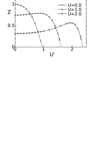
Figure 1: The quasi-particle weight $Z$ as a function of the interorbital Coulomb interaction $U^{\prime}$. The data are obtained by the ED $(N=6)$ within DMFT.

For $U=0$, $Z$ decreases monotonically with increasing $U^{\prime}$, and a metal-insulator transition occurs around $U^{\prime}_{c}\sim 0.9$. On the other hand, when $U\neq 0$, there appears nonmonotonic behavior in $Z$; it once increases with the increase of $U^{\prime}$, has the maximum value in the vicinity of $U^{\prime}\sim U$, and finally vanishes at the Mott transition point. It is somehow unexpected that the maximum structure appears around $U\sim U^{\prime}$, which is more enhanced for larger $U$ and $U^{\prime}$. We will see below that this is related to enhanced orbital fluctuations. By repeating similar calculations systematically, we end up with the phase diagram at zero temperature (Fig. 2), where the contour plot of the quasi-particle weight is shown explicitly.

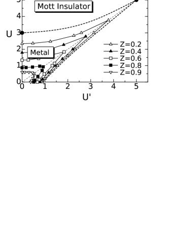
Figure 2: The zero-temperature phase diagram for $J=0$. The contour plot of the quasi-particle weight $Z$ is shown: the bold-dashed line represents the phase boundary of the metal-insulator transition, which is obtained by estimating the values of $U$ and $U^{\prime}$ that give $Z=0$. The solid circles are the transition points obtained by the linearized DMFT.[75]

At $U^{\prime}=0$, where the system is reduced to the single-orbital Hubbard model, we find that the intraorbital Coulomb interaction $U$ triggers the metal-insulator transition at $U_{c}=2.9\sim 3.0$. This critical value obtained by the ED of a small system $(N=6)$ is in good agreement with other numerical calculations such as the numerical renormalization group $(U_{c}=2.94)$,[73, 81] the ED $(U_{c}=2.93)$,[77] the linearized DMFT $(U_{c}=3)$,[75, 76] the dynamical density-matrix renormalization group $(U_{c}=3.07)$.[80, 82]

There are some notable features in the phase diagram. First, the value of $Z$ is not so sensitive to $U^{\prime}$ for a given $U$ ($>U^{\prime}$), except for the region $U\sim U^{\prime}$. In particular, the phase boundary indicated by the dashed line in the upper side of the figure is almost flat for the small $U$ region. The second point is that when $U\sim U^{\prime}$ the metallic phase is stabilized up to fairly large Coulomb interactions, and it becomes unstable, once the parameters are away from the condition $U=U^{\prime}$. The latter tendency is more conspicuous in the regime of strong correlations. [33, 24]

3.2 finite-temperature properties

To observe such characteristic properties around $U=U^{\prime}$ in more detail, we compute the physical quantities at finite temperatures by exploiting the QMC method as an impurity solver.[95] In Fig. 3, we show the DOS deduced by applying the maximum entropy method (MEM) [97, 98, 99] to the Monte Carlo data.[36]

Figure 3: The DOS for the two-orbital Hubbard model $(U=3.0)$. The data are for the inverse temperature $T^{-1}=1,2,4,8$ and $16$ from the top to the bottom.

In the case $(U,U^{\prime})=(3.0,0.0)$, the system is in the insulating phase close to the transition point (see Fig.2). Nevertheless we can clearly observe the formation of the Hubbard gap with the decrease of temperature $T$. In the presence of $U^{\prime}$, the sharp quasi-particle peak is developed around the Fermi level at low temperatures (see the case of $(U,U^{\prime})=(3.0,3.0)$). This implies that orbital fluctuations induced by $U^{\prime}$ drive the system to the metallic phase. Further increase in the interorbital interaction suppresses spin fluctuations, leading the system to another type of the Mott insulator in the region of $U^{\prime}>U$.

To characterize the nature of the spin and orbital fluctuations around the Mott transition, we investigate the temperature dependence of the local spin and orbital susceptibilities, which are defined as,

$$\chi_{s} = \int_{0}^{\beta}{\rm d}\tau\langle\left\{n_{\uparrow}(0)-n_{\downarrow}(0)\right\}\left\{n_{\uparrow}(\tau)-n_{\downarrow}(\tau)\right\}\rangle$$

$$\chi_{o} = \int_{0}^{\beta}{\rm d}\tau\langle\left\{n_{1}(0)-n_{2}(0)\right\}\left\{n_{1}(\tau)-n_{2}(\tau)\right\}\rangle,$$ (12)

where $\beta=T^{-1}$, $n_{\sigma}=\sum_{\alpha}n_{\alpha,\sigma}$, $n_{\alpha}=\sum_{\sigma}n_{\alpha,\sigma}$ and $\tau$ is imaginary time. We show the results obtained by QMC simulations within DMFT in Fig. 4.

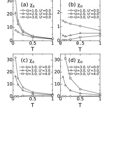
Figure 4: The local spin and orbital susceptibilities as a function of the temperature.

Let us first look at Figs. 4 (a) and (b) for $U^{\prime}=0$ (equivalent to the single-orbital model). Since the introduction of the intraorbital interaction $U$ makes the quasi-particle peak narrower, it increases the spin susceptibility $\chi_{s}$ at low temperatures. On the other hand, the formation of the Hubbard gap suppresses not only the charge susceptibility but also the orbital susceptibility $\chi_{o}$. As seen from Figs. 4 (c) and (d), quite different behavior appears in the susceptibilities, when the interorbital interaction $U^{\prime}$ is increased. Namely, the spin susceptibility is suppressed, while the orbital susceptibility is enhanced at low temperatures. This tendency holds for larger $U^{\prime}$ beyond the condition $U^{\prime}\sim U$. Therefore in the metallic phase close to the Mott insulator in the region of $U>U^{\prime}(U<U^{\prime})$, spin (orbital) fluctuations are enhanced whereas orbital (spin) fluctuations are suppressed with the decrease of the temperature. These analyses clarify why the metallic phase is particularly stable along the line $U=U^{\prime}$. Around this line, spin and orbital fluctuations are almost equally enhanced, and this subtle balance is efficient to stabilize the metallic phase. When the ratio of interactions deviates from this condition, the system prefers either of the two Mott insulating phases.

3.3 phase diagram at finite temperatures

QMC simulations are not powerful enough to determine the phase diagram at finite temperatures. To overcome this difficulty, we make use of a complementary method, SFA,[40] which allows us to discuss the Mott transition at finite temperatures. The obtained phase diagram is shown in Fig. 5, where not only the case of $J=0$ but also $J=0.1U$ are studied under the condition $U=U^{\prime}+2J$.

Figure 5: The finite temperature phase diagram for the two-orbital Hubbard model for $J=0$ and $J=0.1U$ under the condition $U=U^{\prime}+2J$.

It should be noted that the Mott transition at finite temperatures is of first order, similarly to the single-orbital Hubbard case.[3] The critical value for the transition point, $U_{c}$, is determined by comparing the grand potential for each phase. We find the region in the phase diagram where the metallic and Mott insulating phases coexist. Starting from the metallic phase at low temperatures, the increase of the Coulomb interaction triggers the Mott transition to the insulating phase at $U_{c2}$, where we can observe the discontinuity in the quasi-particle weight $Z$. On the other hand, the Mott transition occurs at $U_{c1}$ when the interaction decreases. The phase boundaries $U_{c}$, $U_{c1}$ and $U_{c2}$ merge to the critical temperature $T_{c}$, where the second order transition occurs.

Note that upon introducing the Hund coupling $J$, the phase boundaries are shifted to the weak-interaction region, and therefore the metallic state gets unstable for large $U$. Also, the coexistence region surrounded by the first order transitions shrinks as $J$ increases. This tendency reflects the fact that the metallic state is stabilized by enhanced orbital fluctuations around $U=U^{\prime}$: the Hund coupling suppresses such orbital fluctuations, and stabilizes the Mott-insulating phase. Another remarkable point is that the Mott transition becomes of first-order even at zero temperature in the presence of $J$,[24, 35, 38] since the subtle balance realized at $T=0$ in the case of $U=U^{\prime}$ is not kept anymore for finite $J$. There is another claim that the second order transition could be possible for certain choices of the parameters at $T=0$,[38] so that more detailed discussions may be necessary to draw a definite conclusion on this problem.

4 Orbital-selective Mott transitions

In the previous section, we investigated the two-orbital Hubbard model with same bandwidths, and found that the metallic state is stabilized up to fairly large Coulomb interactions around $U=U^{\prime}$, which is shown to be caused by the enhanced spin and orbital fluctuations. We now wish to see what will happen if we consider the system with different bandwidths, which may be important in real materials such as $\rm Ca_{2-x}Sr_{x}RuO_{4}$[42] and $\rm La_{n+1}Ni_{n}O_{3n+1}$.[56, 55] In the following, we will demonstrate that the enhanced spin and orbital fluctuations again play a key role in controlling the nature of the Mott transitions even for the system with different bandwidths.[14, 15, 20]

4.1 zero-temperature properties

Let us start with the quasi-particle weight calculated by DMFT with the ED method [14] and see the stability of the metallic phase at zero temperature. Here, we include the Hund coupling explicitly under the constraint $U=U^{\prime}+2J$. The quasi-particle weights obtained with fixed ratios $U^{\prime}/U$ and $J/U$ are shown in Fig. 6 for half-filled bands.

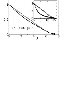
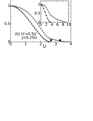
Figure 6: The quasi-particle weights $Z_{1}$ and $Z_{2}$ at half filling as a function of $U$ for $D_{1}=1.0$ and $D_{2}=2.0$: (a) $U^{\prime}/U=1.0$ ($J=0$) and (b) $U^{\prime}/U=0.5$ ($J/U=0.25$). Open (closed) circles represent the results for orbital $\alpha=1(2)$ obtained by combining DMFT the ED as an impurity solver for the $N=6$ small cluster. Solid triangles represent the Mott-transition points obtained by the two-site DMFT method. Insets show the same plots for $D_{1}=1.0$ and $D_{2}=5.0$.

We first study the case of $U=U^{\prime}$ and $J=0$ with bandwidths $D_{1}=1.0$ and $D_{2}=2.0$ [Fig. 6 (a)]. When the Coulomb interaction is switched on, the quasi-particle weights $Z_{1}$ and $Z_{2}$ decrease from unity in slightly different manners reflecting the different bandwidths. A strong reduction in the quasi-particle weight appears initially for the narrower band. However, as the system approaches the Mott transition, the quasi-particle weights merge again, exhibiting very similar $U$-dependence, and eventually vanish at the same critical value. This behavior is explained as follows. For small interactions, the quasi-particle weight depends on the effective Coulomb interactions $U/D_{\alpha}$ which are different for two bands of different width $D_{\alpha}$, and give distinct behavior of $Z_{1}$ and $Z_{2}$. However, in the vicinity of the Mott transition, the effect of the bare bandwidth is diminished due to the strong renormalization of the effective quasi-particle bandwidth, allowing $Z_{1}$ and $Z_{2}$ to vanish together [100, 101].

The introduction of a finite Hund coupling $J$ makes $U\neq U^{\prime}$, and causes qualitatively different behavior [Fig. 6 (b)]. As $U$ increases with the fixed ratio $U^{\prime}/U=0.5$, the quasi-particle weights decrease differently and vanish at different critical points: $U_{c1}\approx 2.6$ for $Z_{1}$ and $U_{c2}\approx 3.5$ for $Z_{2}$. We thus have an intermediate phase with one orbital localized and the other itinerant, which may be referred to as the intermediate phase. The analogous behavior is observed for other choices of the bandwidths, if $J$ takes a finite value [see the inset of Fig. 6 (b)]. These results certainly suggest the existence of the OSMT with $U_{c2}>U_{c1}$.

We have repeated similar DMFT calculations for various choices of the parameters to determine the ground-state phase diagram, which is shown in Fig. 7.

Figure 7: The zero-temperature phase diagram for two-orbital Hubbard model for $D_{1}=1$ and $D_{2}=2$. In the phase (I) [phase (II)], both bands are in metallic (insulating) state. The phase (III) is induced by the OSMT, where the metallic state coexists with the Mott insulating state. Since we consider the ferromagnetic Hund coupling, $J>0$, the relevant region in the diagram is $U>U^{\prime}$.

The phase diagram has some remarkable features. First, the metallic phase (I) is stabilized up to fairly large Coulomb interaction $U$ when $U\to U^{\prime}$ (small $J$). Here the Mott transitions merge to a single transition. As mentioned above, this behavior reflects the high symmetry in the case of $U=U^{\prime}$ ($J=0$) with six degenerate two-electron onsite configurations: four spin configurations with one electron in each orbital and two spin singlets with both electrons in one of the two orbitals. Away from the symmetric limit, i.e. $U>U^{\prime}$ ($2J=U-U^{\prime}$) orbital fluctuations are suppressed and the spin sector is reduced by the Hund coupling to three onsite spin triplet components as the lowest multiplet for two-electron states. In this case, we encounter two types of the Mott transitions having different critical points. In between the two transitions we find the intermediate OSM phase (III) with one band localized and the other itinerant. Within our DMFT scheme we have confirmed that various choices of bandwidths give rise to the qualitatively same structure of the phase diagram as shown in Fig. 7 (see also the discussions in Summary).

4.2 finite-temperature properties

To clarify how enhanced orbital fluctuations around $U=U^{\prime}$ affect the nature of Mott transitions,

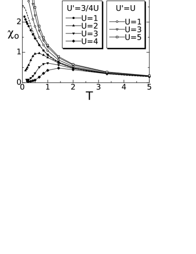
Figure 8: The orbital susceptibility as a function of $T$ for $V=0$. Open (solid) symbols represent the results in the case $U=U^{\prime}$ and $J=0$ ($U^{\prime}/U=3/4$ and $J/U=1/8$) and dashed lines those for the non-interacting case.

let us study the temperature-dependent orbital susceptibility, which is shown in Fig. 8. Here, we have used the new algorithm of the QMC simulations proposed by Sakai et al.[37] to correctly take into account the effect of Hund coupling including the exchange and the pair hopping terms.[15]

We can see several characteristic properties in Fig. 8. In the non-interacting system, the orbital susceptibility increases with decreasing temperature, and reaches a constant value at zero temperature. When the interactions are turned on ($U^{\prime}/U=3/4$ and $J/U=1/8$), the orbital susceptibility is suppressed at low temperatures, which implies that electrons in each band become independent. Eventually for $U\geq U_{c1}\sim 3$, one of the orbitals is localized, so that orbital fluctuations are suppressed completely, giving $\chi_{o}=0$ at $T=0$. On the other hand, quite different behavior appears around $U^{\prime}=U$. In this case, the orbital susceptibility is increased with the increase of interactions even at low temperatures. Comparing this result with the phase diagram in Fig. 7, we can say that the enhanced orbital fluctuations are relevant for stabilizing the metallic phase in the strong correlation regime. While such behavior has been observed for models with two equivalent orbitals (previous section), it appears even in the systems with nonequivalent bands.[36]

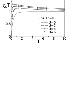
Figure 9: (a) The effective Curie constant $\chi_{s}T$ as a function of $T$ for $U^{\prime}/U=3/4$ and $J/U=1/8$; (b) the results for $U^{\prime}=U$ and $J=0$.

In Fig. 9, the effective Curie constant $\chi_{s}T$ is shown as a function of the temperature. We first look at the case of $U^{\prime}/U=3/4$ and $J/U=1/8$. At high temperatures, all the spin configurations are equally populated, so that the effective Curie constant has the value $1/2$ for each orbital in our units, giving $\chi_{s}T\sim 1$. For weak electron correlations ($U=1$), the system is in the metallic phase, so that the Pauli paramagnetic behavior appears, resulting in $\chi_{s}T\rightarrow 0$ as $T\rightarrow 0$. We can see that the increase of the interactions enhances the spin susceptibility at low temperatures, as a result of the progressive trend to localize the electrons. The effective Curie constant is $\chi_{s}T=2$ when a free spin is realized in each orbital, while $\chi_{s}T=8/3$ when a triplet $S=1$ state is realized due to the Hund coupling. It is seen that the Curie constant increases beyond these values with the increase of the interactions ($U=3,4$). This means that ferromagnetic correlations due to the Hund coupling appear here.

For $U^{\prime}=U$, we can confirm that not only orbital but also spin fluctuations are enhanced in the presence of the interactions, see Fig. 9 (b). Accordingly, both spin and orbital susceptibilities increase at low temperatures, forming heavy-fermion states as far as the system is in the metallic phase. Note that for $U=6$, at which the system is close to the Mott transition point, the spin susceptibility is enhanced with the effective Curie constant $\chi_{s}T\sim 4/3$ down to very low temperatures [Fig. 9 (b)]. The value of 4/3 originates from two additional configurations of doubly-occupied orbital besides four magnetic configurations, which are all degenerate at the metal-insulator transition point. Although not clearly seen in the temperature range shown, the Curie constant $\chi_{s}T$ should vanish at zero temperature for $U=U^{\prime}=6$, since the system is still in the metallic phase, as seen from Fig. 7.

Figure 10: Solid (dashed) lines represent the DOS for the orbital $\alpha=1$ ($\alpha=2$) when $(D_{1},D_{2})=(1.0,2.0)$. The data are for the temperatures $T=2,1,1/2$ and $1/6$ from the top to the bottom.

To see how the above spin and orbital characteristics affect one-electron properties, we show the DOS for each orbital in Fig. 10, which is computed by the MEM.[97, 98, 99] When the interactions increase along the line $U^{\prime}/U=3/4$ and $J/U=1/8$, the OSMT should occur. Such tendency indeed appears at low temperatures in Fig. 10(a). Although both orbitals are in metallic states down to low temperatures ($T=1/6$) for $U=1$, the OSMT seems to occur for $U=2$; one of the bands develops the Mott Hubbard gap, while the other band still remains metallic. At a first glance, this result seems slightly different from the ground-state phase diagram shown in Fig. 7, where the system is in the phase (I) even at $U=2$. However, this deviation is naturally understood if we take into account the fact that for $U=2$, the narrower band is already in a highly correlated metallic state, so that the sharp quasi-particle peak immediately disappears as the temperature increases. This explains the behavior observed in the DOS at $T=1/6$. For $U=3$, both bands are insulating at $T=1/6$ (the system is near the boundary between the phases (II) and (III) at $T=0$). For $U^{\prime}=U$, the qualitatively different behavior appears in Fig. 10. In this case, quasi-particle peaks are developed in both bands as the interactions increase, and the system still remains metallic even at $U=U^{\prime}=3$. As mentioned above, all these features, which are contrasted to the case of $U^{\prime}\neq U$, are caused by equally enhanced spin and orbital fluctuations around $U=U^{\prime}$.

4.3 phase diagram at finite temperatures

Having studied the spin and orbital properties, we now obtain the phase diagram at finite temperatures in the general case $U\neq U^{\prime}$ and $J\neq 0$. Since each Mott transition at zero temperature is similar to that for the single-orbital Hubbard model, [3] we naturally expect that the transition should be of first order at finite temperatures around each critical point [11]. In fact, we find the hysteresis in the physical quantities. For example, we show the entropy per site in Fig. 11.

Figure 11: The entropy as a function of $U$ at $T=0.002,J=0.25U$.

At $T=0.002$, when $U$ increases, the metallic state (I) disappears around $U_{c2}\sim 2.36$ where the first-order Mott transition occurs to the intermediate phase (III), which is accompanied by the jump in the curve of entropy. On the other hand, as $U$ decreases, the intermediate phase (III) is stabilized down to $U_{c1}\sim 2.24$. The first-order critical point $U_{c}\sim 2.33$ for $T=0.002$ is estimated by comparing the grand potential for each phase.[20] The phase diagram thus obtained by SFA is shown in Fig. 12.

Figure 12: The finite-temperature phase diagram for $J=0.25U$. There are two coexistence phases, which correspond to the triangular-shaped regions: the metallic phase and the intermediate phase coexist in the left region and the intermediate phase and insulating phase coexist in the right region.

It is seen that the two coexistence regions appear around $U\sim 2.4$ and $U\sim 3.3$. The phase boundaries $U_{c1}$, $U_{c2}$ and $U_{c}$ merge at the critical temperature $T_{c}$ for each transition. We note that similar phase diagram was obtained by Liebsch by means of DMFT with the ED method.[11] Our SFA treatment elucidates further interesting properties such as the crossover behavior among the competing phases (I), (II) and (III). To see this point more clearly, we show the detailed results for the entropy and the specific heat in Fig. 13.

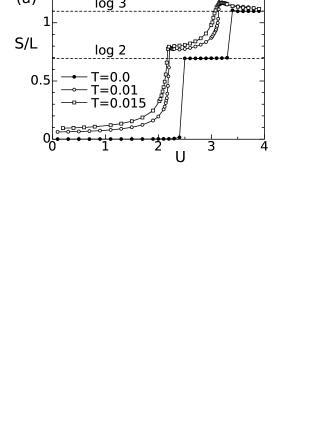
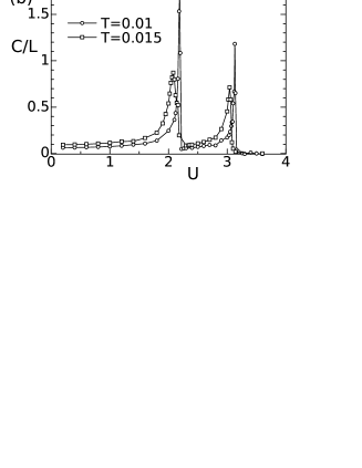
Figure 13: (a) Entropy $S/L$ and (b) Specific heat $C/L$ as a function of $U$ in the crossover region, $J=0.25U$.

There exists a double-step structure in the curve of the entropy, which is similar to that found at $T=0$, where the residual entropy $S/L=0,\log 2$ and $\log 3$ appears in the phase (I), (III) and (II), respectively. Such anomalies are observed more clearly in the specific heat. It is remarkable that the crossover behavior among three phases is clearly seen even at high temperatures. Therefore, the intermediate phase (III) is well defined even at higher temperatures above the critical temperatures.

5 Effect of hybridization between distinct orbitals

In the present treatment of the model with DMFT, the intermediate phase (III) is unstable against certain perturbations. There are several mechanisms that can stabilize this phase. A possible mechanism, which may play an important role in real materials, is the hybridization between the two distinct orbitals. The effect of the hybridization is indeed important, e.g. for the compound $\rm Ca_{2-x}Sr_{x}RuO_{4}$, [42] where the hybridization between $\{\alpha,\beta\}$ and $\gamma$ orbitals is induced by the tilting of RuO₆ octahedra in the region of $\rm Ca$-doping $0.2<x<0.5$[43]. An interesting point is that the hybridization effect could be closely related to the reported heavy fermion behavior.[44, 42] The above interesting aspect naturally motivates us to study the hybridization effect between the localized and itinerant electrons in the intermediate phase (III). Here, we take into account the effect of hybridization in each phase to study the instability of the OSMT.[15, 18]

We study the general case with $U^{\prime}\neq U$ and $J\neq 0$ in the presence of the hybridization $V$. In Fig. 14, we show the DOS calculated by QMC and MEM for several different values of $V$.

Figure 14: Solid (dashed) lines represent the DOS for the orbital $\alpha=1$ ($\alpha=2$) when $(D_{1},D_{2})=(1.0,2.0)$ at $T=1/6$ with the fixed parameters of $U^{\prime}/U=3/4$ and $J/U=1/8$. The data are plotted for $V=0.0,0.25,0.5,0.75,1.0,1.25$ and $1.5$ from top to bottom.

We begin with the case of weak interaction, $U=1$, where the metallic states are realized in both orbitals at $V=0$. Although the introduction of small $V$ does not change the ground state properties, further increase in $V$ splits the DOS, signaling the formation of the band insulator, where all kinds of excitations have the gap. On the other hand, different behavior appears when the interactions are increased up to $U=2$ and 3. In these cases, the system at $V=0$ is in the intermediate or Mott-insulating phase at $T=1/6$. It is seen that the DOS around the Fermi level increases as $V$ increases. At $U=2$, the intermediate state is first changed to the metallic state, where the quasi-particle peaks emerge in both orbitals ($V=0.75,1.0$). For fairly large $V$, the system falls into the renormalized band insulator ($V=1.5$). In the case of $U=3$, the hybridization first drives the Mott-insulating state to the intermediate one, as seen at $V=0.75$, which is followed by two successive transitions.

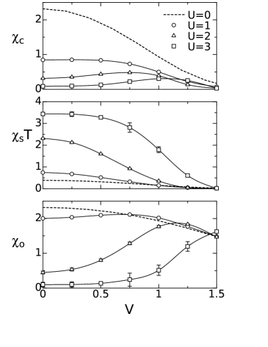
Figure 15: The charge, spin and orbital susceptibilities as a function of $V$ at $T=1/6$.

These characteristic properties are also observed in the charge, spin and orbital susceptibilities at low temperatures (Fig. 15). For weak interactions ($U=1$), the charge susceptibility $\chi_{c}$ monotonically decreases with the increase of $V$. When electron correlations become strong, nonmonotonic behavior appears in $\chi_{c}$: the charge fluctuations, which are suppressed at $V=0$, are somewhat recovered by the hybridization. For large $V$, $\chi_{c}$ is suppressed again since the system becomes a band insulator. It is seen that the orbital susceptibility $\chi_{o}$ shows nonmonotonic behavior similar to the charge susceptibility, the origin of which is essentially the same as in $\chi_{c}$. In contrast, the spin susceptibility decreases with the increase of $V$ irrespective of the strength of the interactions. As is the case for $V=0$, the effective spin is enhanced by ferromagnetic fluctuations due to the Hund coupling in the insulating and intermediate phases. When the hybridization is introduced in these phases, the ferromagnetic fluctuations are suppressed, resulting in the monotonic decrease of the effective Curie constant.

We can thus say that the introduction of appropriate hybridization gives rise to heavy-fermion metallic behavior. Such tendency is observed more clearly in an extreme choice of the bandwidths, $(D_{1},D_{2})=(1.0,10.0)$, as shown in Fig. 16.

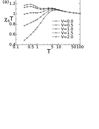
Figure 16: (a) Effective Curie constant as a function of $T$ and (b) DOS in the narrower band $(\alpha=1)$ at $T=1/4$ for an extreme choice of the bandwidths, $(D_{1},D_{2})=(1.0,10.0)$. The DOS for the wider band is not shown here. The other parameters are $U=4.0,U^{\prime}=3.0$ and $J=0.5$.

Since the system is in the intermediate phase at $V=0.0$, the narrower band shows localized-electron properties [Fig. 16 (b)] in the background of the nearly free bands. This double structure in the DOS yields two peaks in the temperature-dependent Curie constant, as shown in Fig. 16 (a). The localized state plays a role of the $f$-state in the Anderson lattice model, [102] so that heavy-fermion quasi-particles appear around the Fermi level for finite $V$, which are essentially the same as those observed in Fig. 14.

Finally, we make some comments on the phase diagram at $T=0$. Although we have not yet studied low-temperature properties in the presence of $V$, we can give some qualitative arguments on the phase diagram expected at zero temperature. As shown above, the metallic phase (I) is not so sensitive to $V$ in the weak-$V$ regime. This is also the case for the insulating phase (II), where a triplet state ($S=1$) formed by the Hund coupling is stable against a weak hybridization. There appears a subtle situation in the intermediate phase (III). The intermediate phase exhibits Kondo-like heavy fermion behavior at low temperatures in the presence of $V$. However, we are now dealing with the half-filled case, so that this Kondo-like metallic phase should acquire a Kondo-insulating gap due to commensurability at zero temperature. Therefore, the intermediate phase (III) should be changed into the Kondo-insulator with a tiny excitation gap in the presence of $V$ at $T=0$. Accordingly, the sharp transition between the phases (II) and (III) at $V=0$ still remains in the weakly hybridized case. [18] This is different from the situation in the periodic Anderson model with the Coulomb interactions for conduction electrons as well as localized $f$ electrons, where the spin-singlet insulating phase is always realized in its parameter range.[90, 87] Consequently we end up with the schematic phase diagram (Fig. 17) for the two-orbital model with the hybridization between the distinct orbitals.

Figure 17: The schematic phase diagram for the model with finite $V$ at $T=0$. Solid lines represent the phase boundaries between the metallic and insulating phases. Dashed line indicates the phase boundary between the Mott insulator and the Kondo insulator.

Recall that the phase has three regions on the line $V=0$: (I) metallic, (II) insulating and (III) intermediate phases. The metallic phase (I) for small $U$ is simply driven to the band-insulator (IV) beyond a certain critical value of $V$. The intermediate phase (III) at $V=0$ is changed to the Kondo-insulator (V) in the presence of any finite $V$. As $V$ increases, this insulating state first undergoes a phase transition to the metallic phase (I), and then enters the band-insulator (IV). On the other hand, the Mott insulating phase (II) first shows a transition to the Kondo insulator (V), which is further driven to the metallic phase (I) and then to the band-insulating phase (IV). Note that at finite temperatures above the Kondo-insulating gap, we can observe Kondo-type heavy fermion behavior in the intermediate phase with finite $V$.

6 Summary

We have investigated the Mott transitions in the two-orbital Hubbard model by means of DMFT and SFA. It has been clarified that orbital fluctuations enhanced in the special condition $U\sim U^{\prime}$ and $J\sim 0$ play a key role in stabilizing the correlated metallic state. In particular, this characteristic property gives rise to nontrivial effects on the Mott transition, which indeed control whether the OSMT is realized in the two-orbital model with different bandwidths.

We have demonstrated the above facts by taking the system with the different bandwidths $(D_{1},D_{2})=(1.0,2.0)$ as an example. In the special case with $U=U^{\prime}$ and $J=0$, the metallic state is stabilized up to fairly large interactions, resulting in a single Mott transition. The resulting single transition is nontrivial, since we are concerned with the system with different bandwidths. On the other hand, for more general cases with $U\neq U^{\prime}$ and $J\neq 0$, the Hund coupling suppresses orbital fluctuations, giving rise to the OSMT. We have confirmed these results by computing various quantities at zero and finite temperatures.

Recently, it was reported that when the ratio of the bandwidths is quite large, the OSMT occurs even in the case of $U=U^{\prime}$ and $J=0$.[18, 17] This result implies that the detailed structure of the phase diagram in some extreme cases depends on the parameters chosen, and is not completely categorized in the scheme discussed in this paper. This naturally motivates us to establish the detailed phase diagrams at zero and finite temperatures by incorporating various effects such as the magnetic field, the crystalline electric field,[13] the lattice structure, etc.

In this paper, we have restricted our discussions to the normal metallic and Mott insulating phases without any long-range order. It is an important open problem to take into account such instabilities to various ordered phases, which is now under consideration.

References

- [1] M. Imada, A. Fujimori and Y. Tokura, Rev. Mod. Phys. 70, 1039 (1998).
- [2] Y. Tokura and N. Nagaosa, Science 288,462 (2000).
- [3] A. Georges, G. Kotliar, W. Krauth and M. J. Rozenberg, Rev. Mod. Phys. 68, 13 (1996).
- [4] W. Metzner and D. Vollhardt, Phys. Rev. Lett. 64, 324 (1989).
- [5] E. Müller-Hartmann, Z. Phys. B, Condens. Matter 74, 507 (1989).
- [6] T. Pruschke, M. Jarrell and J. K. Freericks, Adv. Phys. 44, 187 (1995).
- [7] G. Kotliar and D. Vollhardt, Physics Today 53, (2004).
- [8] A. Liebsch, Europhys. Lett., 63, 97 (2003); Phys. Rev. Lett., 91, 226401 (2003).
- [9] A. Koga, N. Kawakami, T. M. Rice, and M. Sigrist, Physica B 359-361, 1366 (2005).
- [10] C. Knecht, N. Blümer and P. G. J. van Dongen, Phys. Rev. B 72, 081103 (2005).
- [11] A. Liebsch, Phys. Rev. Lett. 95, 116402 (2005).
- [12] S. Biermann, L. de’ Medici and A. Georges, cond-mat/0505737.
- [13] A. Rüegg, M. Indergand, S. Pilgram, and M. Sigrist, cond-mat/0508691.
- [14] A. Koga, N. Kawakami, T.M. Rice and M. Sigrist, Phys. Rev. Lett. 92, 216402 (2004)
- [15] A. Koga, N. Kawakami, T. M. Rice, and M. Sigrist, Phys. Rev. B 72, 045128 (2005).
- [16] Y. Tomio and T. Ogawa, J. Luminesci. 112, 220 (2005).
- [17] M. Ferrero, F. Becca, M. Fabrizio and M. Capone, cond-mat/0503759.
- [18] L. de’ Medici, A. Georges and S. Biermann, cond-mat/0503764.
- [19] R. Arita and K. Held, cond-mat/0504040.
- [20] K. Inaba, A. Koga, S. Suga, N. Kawakami, J. Phys. Soc. Jpn. 74, 2393 (2005).
- [21] A. Georges, G. Kotliar and W. Krauth, Z. Phys. B 92, 313 (1993).
- [22] G. Kotliar and H. Kajueter, Phys. Rev. B 54, 14221 (1996).
- [23] M. J. Rozenberg, Phys. Rev. B 55, 4855 (1997).
- [24] J. Bünemann and W. Weber, Phys. Rev. B 55, 4011 (1997); J. Bünemann and W. Weber and F. Gebhard, Phys. Rev. B 57, 6896 (1998).
- [25] H. Hasegawa, J. Phys. Soc. Jpn. 56, 1196 (1997).
- [26] K. Held and D. Vollhardt, Eur. Phys. J. B 5, 473 (1998).
- [27] J. E. Han, M. Jarrel and D. L. Cox, Phys. Rev. B 58, 4199 (1998).
- [28] T. Momoi and K. Kubo, Phys. Rev. B 58, 567 (1998).
- [29] A. Klejnberg and J. Spalek, Phys. Rev. B 57, 12401 (1998).
- [30] Th. Maier, M. B. Zölfl, Th. Pruschke and J. Keller, Eur. Phys. J. B 7, 377 (1999).
- [31] Y. Imai and N. Kawakami, J. Phys. Soc. Jpn 70, 2365 (2001).
- [32] V. S. Oudovenko and G. Kotliar, Phys. Rev. B 65, 075102 (2002).
- [33] A. Koga, Y. Imai and N. Kawakami, Phys. Rev. B 66, 165107 (2002).
- [34] S. Florens, A. Georges, G. Kotliar and O. Parcollet, Phys. Rev. B 66, 205102 (2002); S. Florens, A. Georges, Phys. Rev. B 66, 165111 (2002).
- [35] Y. Ono, M. Potthoff and R. Bulla, Phys. Rev. B 67, 035119 (2003).
- [36] A. Koga, T. Ohashi, Y. Imai, S. Suga and N. Kawakami, J. Phys. Soc. Jpn. 72, 1306 (2003).
- [37] S. Sakai, R. Arita, and H. Aoki, Phys. Rev. B 70, 172504 (2004).
- [38] T. Pruschke and R. Bulla, Eur. Phys. J. B 44, 217 (2005).
- [39] Y. Song and L.-J. Zou, Phys. Rev. B 72, 085114 (2005).
- [40] K. Inaba, A. Koga, S. Suga, and N. Kawakami, Phys. Rev. B 72, 085112 (2005).
- [41] V.I. Anisimov, I.A. Nekrasov, D.E. Kondakov, T.M. Rice and M. Sigrist, Eur. Phys. J. B 25, 191 (2002).
- [42] S. Nakatsuji and Y. Maeno, Phys. Rev. Lett. 84, 2666 (2000).
- [43] O. Friedt, M. Braden, G. André, P. Adelmann, S. Nakatsuji, and Y. Maeno, Phys. Rev. B 63, 174432 (2001).
- [44] S. Nakatsuji, D. Hall, L. Balicas, Z. Fisk, K. Sugahara, M. Yoshioka, and Y. Maeno, Phys. Rev. Lett. 90, 137202 (2003).
- [45] Y. Maeno, T.M. Rice and M. Sigrist, Physics Today, 54, 42 (2001).
- [46] A.P. Mackenzie and Y. Maeno, Rev. Mod. Phys. 75, 657 (2003).
- [47] S. Nakatsuji, S. I. Ikeda, and Y. Maeno, J. Phys. Soc. Jpn. 66, 1868 (1997).
- [48] M. Braden, G. André, S. Nakatsuji and Y. Maeno, Phys. Rev. B 58, 847 (1998).
- [49] F. Nakamura, T. Goko, M. Ito, T. Fujita, S. Nakatsuji, H. Fukazawa, Y. Maeno, P. Alireza, D. Forsythe, and S. R. Julian, Phys. Rev. B 65, 220402 (2002).
- [50] I. I. Marzin and D. J. Singh, Phys. Rev. Lett. 82, 4324 (1999).
- [51] T. Hotta and E. Dagotto, Phys. Rev. Lett. 88, 017201 (2001).
- [52] Z. Fang and K. Terakura, Phys. Rev. B 64, R020509 (2001); Z. Fang, N. Nagaosa and K. Terakura, Phys. Rev. B 69, 045116 (2004).
- [53] S. Okamoto and A. J. Mills, Phys. Rev. B 70, 195120 (2004).
- [54] M. Sigrist and M. Troyer, Eur. J. Phys. B, 39, 207 (2004).
- [55] K. Sreedhar, M. McElfresh, D. Perry, D. Kim, P. Metcalf and J. M. Honig, J. Solid State Comm. 110, 208 (1994); Z. Zhang, M. Greenblatt and J. B. Goodenough, J. Solid State Comm. 108, 402 (1994); 117, 236 (1995).
- [56] Y. Kobayashi, S. Taniguchi, M. Kasai, M. Sato, T. Nishioka and M. Kontani, J. Phys. Soc. Jpn 65, 3978 (1996).
- [57] M. Potthoff, Eur. Phys. J. B 32, 429 (2003); 36, 335 (2003); K. Pozgǎjčić, cond-mat/0407172.
- [58] Y. Kuramoto, Z. Phys. B 53, 37 (1983).
- [59] P. Coleman, Phys. Rev. B 28, 5255 (1983); 29, 3035 (1984).
- [60] T.M. Rice and K. Ueda, Phys. Rev. Lett. 55, 995 (1985); Phys. Rev. B 34, 6420 (1986).
- [61] C.-I. Kim, Y. Kuramoto and T. Kasuya, J. Phys. Soc. Jpn. 59, 2414 (1990).
- [62] K. Yamada, K. Yosida, and K. Hanzawa, Prog. Thero, Phys. Suppl. 108, 141 (1992).
- [63] H. Tsunetsugu, M. Sigrist and K. Ueda, Rev. Mod. Phys. 69, 809 (1997).
- [64] F. F. Assaad, Phys. Rev. Lett. 83, 796 (1999).
- [65] C. Zener, Phys. Rev. 82, 4031 (1951).
- [66] P. W. Anderson and H. Hasegawa, Phys. Rev. 100, 675 (1955).
- [67] K. Kubo and N. Ohata, J. Phys. Soc. Jpn. 33, 21 (1975).
- [68] N. Furukawa, J. Phys. Soc. Jpn. 64, 2734 (1995).
- [69] Th. Pruschke, D. L. Cox and M. Jarrell, Phys. Rev. B 47, 3553 (1993).
- [70] O. Sakai and Y. Kuramoto, Solid State Comm. 89, 307 (1994).
- [71] M. Caffarel and W. Krauth, Phys. Rev. Lett. 72, 1545 (1994).
- [72] M. J. Rozenberg, G. Kotliar, and X. Y. Zhang, Phys. Rev. B 49, 10181 (1994).
- [73] R. Bulla, Phys. Rev. Lett. 83, 136 (1999); R. Bulla, T. A. Costi, D. Vollhardt, Phys. Rev. Lett. 64, 045103 (2001).
- [74] R. Chitra and G. Kotliar, Phys. Rev. Lett. 83, 2386 (1999).
- [75] R. Bulla and M. Potthoff, Eur. Phys. J. B 13, 257 (2000).
- [76] M. Potthoff, Phys. Rev. B 64, 165114 (2001).
- [77] Y. Ono, R. Bulla and A. C. Hewson, Eur. Phys. J. B 19, 375 (2001); Y. Ohashi and Y. Ono, J. Phys. Soc. Jpn. 70, 2989 (2001).
- [78] J. Joo and V. Oudovenko, Phys. Rev. B 64, 193102 (2001).
- [79] M. S. Laad, L. Craco and E. Müller-Hartmann, Phys. Rev. B 64, 195114 (2001).
- [80] S. Nishimoto, F. Gebhard, and E. Jeckelmann, J. Phys. Condens. Matter 16, 7063 (2004).
- [81] R. Zitzler, N.-H. Tong, Th. Pruschke, and R. Bulla, Phys. Rev. Lett. 93, 016406 (2004).
- [82] M. Karski, C. Raas, and G. S. Uhrig, cond-mat/0507132.
- [83] M. Jarrell, H. Akhlaghpour and T. Pruschke, Phys. Rev. Lett. 70, 1670 (1993).
- [84] T. Mutou and D. Hirashima, J. Phys. Soc. Jpn. 63, 4475 (1994);
- [85] M. J. Rozenberg, Phys. Rev. B 52, 7369 (1995).
- [86] T. Saso and M. Itoh, Phys. Rev. B 53, 6877 (1996);
- [87] T. Schork and S. Blawid, Phys. Rev B 56, 6559 (1997)
- [88] P. Sun and G. Kotliar, Phys. Rev. B 91, 037209 (2003).
- [89] T. Ohashi, A. Koga, S. Suga, and N. Kawakami, Phys. Rev. B 70, 245104 (2004); Physica B 359-361, 738 (2005).
- [90] R. Sato, T. Ohashi, A. Koga, and N. Kawakami, J. Phys. Soc. Jpn. 73, 1864 (2004).
- [91] L. de’ Medici, A. Georges, G. Kotliar, and S. Biermann, Phys. Rev. Lett. 95, 066402 (2005).
- [92] N. Matsumoto and F. J. Ohkawa, Phys. Rev. B 51, 4110 (1995).
- [93] T. Schork, S. Blawid, and J. Igarashi, Phys. Rev. B 59, 9888 (1999).
- [94] T. Ohashi, S. Suga, and N. Kawakami, J. Phys. Condens. Matter 17, 4547 (2005).
- [95] J. E. Hirsch and R. M. Fye, Phys. Rev. Lett. 56, 2521 (1986).
- [96] J. M. Luttinger, Phys. Rev. 118, 1417 (1960).
- [97] S.F. Gull, in Maximum Entropy and Bayesian Methods in Science and Engineering, edited by G. J. Erickson and C. R. Smith (Kluwer Academic, Dordrecht, 1988), p. 53; J. Skilling, p. 45.
- [98] R. N. Silver, D. S. Sivia, and J. E. Gubernatis, Phys. Rev. B 41, 2380 (1990); J. E. Gubernatis, M. Jarrell, R. N. Silver, and D. S. Sivia, Phys. Rev. B 44, 6011 (1991).
- [99] W.F. Press, S.A. Teukolsky, W.T. Vetterling, and B.R. Flannery, Numerical Recipes (Cambridge University Press, Cambridge, England, 1992), p. 809.
- [100] M. C. Gutzwiller, Phys. Rev. 137, A1726 (1965).
- [101] W. F. Brinkman and T. M. Rice, Phys. Rev. B 2, 4302 (1970).
- [102] H. Kusunose, S. Yotsuhashi, and K. Miyake, Phys. Rev. B 62, 4403 (2000).