Resonant inelastic tunneling in molecular junctions

Abstract

Within a phonon-assisted resonance level model we develop a self-consistent procedure for calculating electron transport currents in molecular junctions with intermediate to strong electron-phonon interaction. The scheme takes into account the mutual influence of the electron and phonon subsystems. It is based on the $2^{nd}$ order cumulant expansion, used to express the correlation function of the phonon shift generator in terms of the phonon momentum Green function. Equation of motion (EOM) method is used to obtain an approximate analog of the Dyson equation for the electron and phonon Green functions in the case of many-particle operators present in the Hamiltonian. To zero-order it is similar in particular cases (empty or filled bridge level) to approaches proposed earlier. The importance of self-consistency in resonance tunneling situations (partially filled bridge level) is stressed. We confirm, even for strong vibronic coupling, a previous suggestion concerning the absence of phonon sidebands in the current vs. gate voltage plot when the source-drain voltage is small Mitra .

I Introduction

Molecular electronics is an active area of research with possible technological interest in supplementing currently available $Si$ based electronics via further miniaturization of electronic devices MEB ; AN . Experiments on conduction in molecular junctions are becoming more common Reed ; Bowler . Early experiments focused on the absolute conduction and on trends such as dependence on wire length, molecular structure, and temperature. An intriguing issue is the role played by molecular nuclear motions. Vibronic coupling may lead to rotations, conformational changes, atomic rearrangements, and chemical reactions induced by the electronic current Park ; Ho_conf . It is directly relevant to the junction heating problem and can manifest itself in polaron-type localization effects and inelastic signals in current-voltage spectra. Ho_IETS ; Zhitenev ; Weig ; Natelson ; Ruitenbeck ; Reed_IETS ; Kushmerick ; SelzerMayer While weak inelastic signatures are observed in measurements of conductance with strong electronic coupling between the molecule and leads, stronger vibronic peaks with pronounced phonon sidebands (we use the term phonon to describe any vibrational excitation) may be observed when this coupling is weak. A full Franck-Condon envelope has been observed with weak molecule-electrode interactions at both termini Ho_FC .

Studies of electron-phonon interaction have a long history Mahan , however new points for consideration arise in biased current carrying junctions. The interpretation of electronic transport in molecular junctions has until recently has been made largely in the context of multi-channel scattering problems DiVentra ; Todorov ; Seideman ; NessFisher ; BoncaTrugman ; Troisi , which disregards the influence of the contact population (manifestations of the Pauli principle blocking of scattering channels, change of electronic structure, etc.) on inelastic process. Such approaches also disregard the influence of the electronic subsystem on the phonon dynamics. A systematic framework describing transport phenomena of many-particle systems which can take these effects into account can be developed based on the non-equilibrium Green’s function (NEGF) formulationKeldysh ; DattaBook ; HaugJauho .

Phonon-assisted electron transport in molecular systems can be classified by the relative time and energy scales of the processes involved. The electron lifetime in the junction should be compared to the relevant vibrational frequencyBurin , while the strength of the electron-phonon coupling should be judged relative to electronic matrix elements (coupling to contacts and/or between isolated parts of the molecular system). It is useful to consider separately the limits of weak and strong electron-phonon coupling. The first corresponds to non-resonant phonon-assisted electron tunneling mostly encountered in experiments on inelastic electron tunneling spectroscopy (IETS) Ho_IETS ; Reed_IETS ; Kushmerick ; SelzerMayer ; Bayman . With the development and advances in scanning tunneling microscopy (STM) and scanning tunneling spectroscopy (STS), IETS has proven invaluable as a tool for identifying and characterizing molecular species within the conduction region. The use of Migdal-Eliashberg theoryME ; FetterWalecka is justified in this case, whereupon the lowest non-vanishing (second) order perturbation in electron-phonon coupling on the Keldysh contour leads to the Born approximation (BA) for electron dynamics. This approach using BA or its self-consistent (in electron Green function) flavor was used in several theoretical studies Ehrenreich ; Hershfield ; Datta ; Ueba ; Pecchia ; Mitra ; Yamamoto . In a recent publication IETS_SCBA we used an advanced version of this scheme, self-consistent Born approximation (SCBA) for both electron and phonon Green functions, to describe features (peaks, dips, line shape, and line width) of the IETS signal, $d^{2}I/d\Phi^{2}$, as a function of the applied voltage $\Phi$. Sometimes SCBA is used also in the resonant tunneling regime Mitra ; Keller . This usage is valid only if electron-phonon interaction is weak, so that no essential inelastic features (e.g. polaron formation) can be studied in this case.

The other limit is realized in cases of resonant tunneling, which is characterized by longer electron lifetime in the junction (though it still may be short relative to the characteristic phonon frequency) and stronger effective electron-phonon coupling. The perturbative treatment breaks down in this case which may result in formation of a polaron in the junction. Signatures of resonant tunneling driven by an intermediate molecular ion appear as peaks in the first derivative $dI/d\Phi$ and may show phonon subbands mceuen ; ralph ; natelson . Several theoretical studies of this situation in tunneling junctions are available NessFisher ; BoncaTrugman ; Wingreen ; Lundin ; Balatsky ; Bratkovsky . Most of them NessFisher ; BoncaTrugman ; Wingreen are based on scattering theory consideration, others Lundin ; Balatsky ; Bratkovsky are based partially on the NEGF methodology. However these works disregard the Fermi population in the leads as mentioned above. Another approach, the non-equilibrium linked cluster expansion (NLCE), is based on generalization of the linked cluster expansion to nonequilibrium situations Kral . This approach takes the contact population into account, but appears to be unstable for diagrammatic expansion beyond the lowest order. Note also that in all the cases mentioned above the phonon subsystem is assumed to remain in thermal equilibrium throughout the process. The rate equations approach often used in the literature for the case of weak coupling to the leads Mitra ; BraigFlensberg ; vonOppen is essentially a quasiclassical treatment, having an assumption that the tunneling rate is much smaller than decoherence rates on the molecular subsystem. While the approach is useful in describing e.g. $C_{60}$ center of mass motion as is done in Ref. BraigFlensberg, , the intramolecular vibrations we are interested in here may have a much longer lifetime, thus making the rate equations approach inappropriate. An attempt to generalize single particle approximation of Refs. Lundin, ; Balatsky, ; Bratkovsky, was presented in Ref. Flensberg, , where an EOM method was used. Another interesting approach uses numerical renormalization group methodology to study inelastic effects in conductance in the linear response regime Cornaglia .

In this paper we propose an approximate scheme for treating electronic transport in cases involving intermediate to strong electron-phonon coupling in tunnel junctions. We employ the Keldysh contour based description, which treats both electron and phonon degrees of freedom in a self-consistent manner. This approach is close in spirit to NLCE Kral in using a cumulant expansion (when finding an approximate expression for phonon shift operators correlation function in terms of phonon Green functions). However unlike NLCE the proposed scheme is stable and self-consistent, i.e. the influence of tunneling current on the phonon subsystem is taken into account. It reduces to the scattering theory results in the limit where the molecular bridge energies are far above the Fermi energy of the leads and provides a scheme for analyzing the effect of the electronic current on the energetics in the vibrational space in resonance tunneling situations (the issue will be discussed elsewhere). Derivation of equations is based on EOM method, which makes our approach similar to Ref. Flensberg, . However we go beyond it in taking into account renormalization of phonon subsystem due to coupling to tunneling electron. Thermal relaxation of the molecular phonons, not taken into account in Flensberg , is also introduced in our consideration.

In the next section we introduce the model and describe the approximations made. Section III presents the procedure of our self-consistent calculation. In section IV we report numerical results and compare them to results obtained within other approaches. Section V concludes.

II Model

We consider a simple resonant-level model with the electronic level $|0>$ coupled to two electrodes left ($L$) and right ($R$) (each a free electron reservoir at its own equilibrium). The electron on the resonant level (electronic energy $\varepsilon_{0}$) is linearly coupled to a single vibrational mode (phonon) with frequency $\omega_{0}$, henceforth referred to as the “primary phonon”. The latter is coupled to a phonon bath represented as a set of independent harmonic oscillators. The system Hamiltonian is (here and below we use $\hbar=1$ and $e=1$)

$$\hat{H}=\varepsilon_{0}\hat{c}^{\dagger}\hat{c}+\sum_{k\in\{L,R\}}\varepsilon_{k}\hat{c}_{k}^{\dagger}\hat{c}_{k}+\sum_{k\in\{L,R\}}\left(V_{k}\hat{c}_{k}^{\dagger}\hat{c}+\mbox{h.c.}\right)$$

$$+\omega_{0}\hat{a}^{\dagger}\hat{a}+\sum_{\beta}\omega_{\beta}\hat{b}^{\dagger}_{\beta}\hat{b}_{\beta}+M_{a}\hat{Q}_{a}\hat{c}^{\dagger}\hat{c}+\sum_{\beta}U_{\beta}\hat{Q}_{a}\hat{Q}_{\beta}$$ (1)

where $\hat{c}^{\dagger}$ ($\hat{c}$) are creation (destruction) operators for electrons on the bridge level, $\hat{c}_{k}^{\dagger}$ ($\hat{c}_{k}$) are corresponding operators for electronic states in the contacts, $\hat{a}^{\dagger}$ ($\hat{a}$) are creation (destruction) operators for the primary phonon, and $\hat{b}_{\beta}^{\dagger}$ ($\hat{b}_{\beta}$) are the corresponding operators for phonon states in the thermal (phonon) bath. $\hat{Q}_{a}$ and $\hat{Q}_{\beta}$ are phonon displacement operators

$$\hat{Q}_{a}=\hat{a}+\hat{a}^{\dagger}\qquad\hat{Q}_{\beta}=\hat{b}_{\beta}+\hat{b}_{\beta}^{\dagger}$$ (2)

The energy parameters $M_{a}$ and $U_{\beta}$ correspond to the vibronic and the vibrational coupling respectively. For future reference we also introduce the phonon momentum operators

$$\hat{P}_{a}=-i\left(\hat{a}-\hat{a}^{\dagger}\right)\qquad\hat{P}_{\beta}=-i\left(\hat{b}_{\beta}-\hat{b}_{\beta}^{\dagger}\right)$$ (3)

In what follows we will refer to the phonon mode $a$ that is directly coupled to the electronic system as the “primary phonon”.

Following previous work on strong electron-phonon interaction Lundin ; Balatsky ; Bratkovsky we start by applying a small polaron (canonical or Lang-Firsov) transformation Mahan ; LangFirsov to the Hamiltonian (II)

$$\hat{\bar{H}}=e^{\hat{S}_{a}}\hat{H}e^{-\hat{S}_{a}}$$ (4)

with

$$\hat{S}_{a}=\frac{M_{a}}{\omega_{0}}\left(\hat{a}^{\dagger}-\hat{a}\right)\hat{c}^{\dagger}\hat{c}$$ (5)

Under the additional approximation of neglecting the effect of this transformation on the coupling of the primary phonon to the thermal phonon bath this leads to

$$\hat{\bar{H}} = \bar{\varepsilon}_{0}\hat{c}^{\dagger}\hat{c}+\sum_{k\in\{L,R\}}\varepsilon_{k}\hat{c}_{k}^{\dagger}\hat{c}_{k}+\sum_{k\in\{L,R\}}\left(V_{k}\hat{c}_{k}^{\dagger}\hat{c}\hat{X}_{a}+\mbox{h.c.}\right)$$ (6)

$$+ \omega_{0}\hat{a}^{\dagger}\hat{a}+\sum_{\beta}\omega_{\beta}\hat{b}^{\dagger}_{\beta}\hat{b}_{\beta}+\sum_{\beta}U_{\beta}\hat{Q}_{a}\hat{Q}_{\beta}$$

where

$$\bar{\varepsilon}_{0}=\varepsilon_{0}-\Delta\qquad\Delta\approx\frac{M_{a}^{2}}{\omega_{0}};$$ (7)

$\Delta$ is the electron level shift due to coupling to the primary phonon and

$$\hat{X}_{a}=\exp\left[i\lambda_{a}\hat{P}_{a}\right]\qquad\lambda_{a}=\frac{M_{a}}{\omega_{0}}$$ (8)

is primary phonon shift generator. The Hamiltonian (6) is characterized by the absence of direct electron-phonon coupling present in (II). This is replaced by renormalization of coupling to the contacts. Note that the same result can be obtained by repeatedly applying the transformation analogous to (5) in the case of weak coupling between primary phonon and thermal bath and neglecting renormalization due to thermal bath phonons (see Appendix A).

The Hamiltonian (6) is our starting point for the calculation of the steady-state current across the junction, using the NEGF expression derived in Refs. HaugJauho, ; current,

$$I_{K}=\frac{e}{\hbar}\int\frac{dE}{2\pi}\left[\Sigma_{K}^{<}(E)\,G^{>}(E)-\Sigma_{K}^{>}(E)\,G^{<}(E)\right]$$ (9)

Here $\Sigma_{K}^{<,>}$ are lesser/greater projections of the self-energy due to coupling to the contact $K$ ($K=L,R$)

$$\Sigma_{K}^{<}(E) = if_{K}(E)\Gamma_{K}(E)$$ (10)

$$\Sigma_{K}^{>}(E) = -i[1-f_{K}(E)]\Gamma_{K}(E)$$ (11)

with $f_{K}(E)$ the Fermi distribution in the contact $K$ and

$$\Gamma_{K}(E)=2\pi\sum_{k\in K}|V_{k}|^{2}\delta(E-\varepsilon_{k})$$ (12)

The lesser and greater Green functions in (9) are Fourier transforms to energy space of projections onto the real time axis of the electron Green function on the Keldysh contour

$$G(\tau_{1},\tau_{2}) =-i<T_{c}\hat{c}(\tau_{1})\hat{c}^{\dagger}(\tau_{2})>_{H}$$

$$=-i<T_{c}\hat{c}(\tau_{1})\hat{X}_{a}(\tau_{1})\,\hat{c}^{\dagger}(\tau_{2})\hat{X}_{a}^{\dagger}(\tau_{2})>_{\bar{H}}$$ (13)

where the subscripts $H$ and $\bar{H}$ indicate which Hamiltonian, (II) or (6) respectively, determines evolution of the system, and $T_{c}$ is the contour ordering operator. We use the second form and make the usual approximation of decoupling electron and phonon dynamics

$$G(\tau_{1},\tau_{2})\approx G_{c}(\tau_{1},\tau_{2})\,K(\tau_{1},\tau_{2})$$ (14)

where

$$G_{c}(\tau_{1},\tau_{2}) = -i<T_{c}\hat{c}(\tau_{1})\hat{c}^{\dagger}(\tau_{2})>_{\bar{H}}$$ (15)

$$K(\tau_{1},\tau_{2}) = <T_{c}\hat{X}_{a}(\tau_{1})\hat{X}_{a}^{\dagger}(\tau_{2})>_{\bar{H}}$$ (16)

Below we drop the subscript $\bar{H}$ keeping in mind that Hamiltonian (6) is the one that determines the time evolution of the system. Previous studies (see e.g. Lundin ; Balatsky ; Bratkovsky ) stopped here and approximated the functions $G_{c}$ and $K$ by the electron Green function in the absence of coupling to phonons and by the equilibrium correlation function of the phonon shift generator $\hat{X}_{a}$, respectively. Here we go a step further by ’dressing’ these terms in the spirit of standard diagrammatic technique Mahan . This will yield a self-consistent approach for the intermediate to strong electron-phonon interaction, the strong coupling analog of the self-consistent Born approximation (SCBA) used in the weak coupling limit IETS_SCBA .

We start by expressing the shift generator correlation function $K$ in terms of the phonon Green function. One can show (see Appendix B) that in the second order cumulant expansion this connection is

$$K(\tau_{1},\tau_{2})=\exp\left\{\lambda_{a}^{2}\left[iD_{P_{a}P_{a}}(\tau_{1},\tau_{2})-<\hat{P}_{a}^{2}>\right]\right\}$$ (17)

where $\hat{P}_{a}$ is the primary phonon momentum operator defined in (3) and

$$D_{P_{a}P_{a}}(\tau_{1},\tau_{2})=-i<T_{c}\hat{P}_{a}(\tau_{1})\hat{P}_{a}(\tau_{2})>$$ (18)

is the phonon momentum Green function. $<\hat{P}_{a}^{2}>=iD_{P_{a}P_{a}}^{<,>}(t,t)$ is time independent in steady-state.

Next we derive self-consistent equations for the electron Green function $G_{c}(\tau_{1},\tau_{2})$, Eq.(15), and the phonon momentum Green function $D_{P_{a}P_{a}}(\tau_{1},\tau_{2})$, Eq. (18). Since we consider situations where the electron-phonon coupling is strong relative to the coupling between the bridge electronic level and the contacts it is reasonable to look for an expression of second order in $V_{k}$. We use an equation of motion (EOM) method to obtain expressions for these Green functions. Since the Hamiltonian (6) contains the exponential operator $\hat{X}$, Wick’s theorem is not applicable so we cannot write the Dyson equations to express these Green functions in terms of the corresponding self-energies. It is nevertheless possible to obtain the following approximate coupled integral equations for these Green functions (see Appendices C and D)

$$D_{P_{a}P_{a}}(\tau,\tau^{\prime})=D_{P_{a}P_{a}}^{(0)}(\tau,\tau^{\prime})$$ (19)

$$+\int_{c}d\tau_{1}\int_{c}d\tau_{2}\,D_{P_{a}P_{a}}^{(0)}(\tau,\tau_{1})\,\Pi_{P_{a}P_{a}}(\tau_{1},\tau_{2})\,D_{P_{a}P_{a}}^{(0)}(\tau_{2},\tau^{\prime})$$

$$G_{c}(\tau,\tau^{\prime})=G_{c}^{(0)}(\tau,\tau^{\prime})$$ (20)

$$+\sum_{K=\{L,R\}}\int_{c}d\tau_{1}\int_{c}d\tau_{2}\,G_{c}^{(0)}(\tau,\tau_{1})\,\Sigma_{c,K}(\tau_{1},\tau_{2})\,G_{c}^{(0)}(\tau_{2},\tau^{\prime})$$

where the functions $\Pi_{P_{a}P_{a}}$ and $\Sigma_{c,K}$ are given by

$$\Pi_{P_{a}P_{a}}(\tau_{1},\tau_{2})=\sum_{\beta}|U_{\beta}|^{2}D_{P_{\beta}P_{\beta}}(\tau_{1},\tau_{2})-i\lambda_{a}^{2}\sum_{k\in\{L,R\}}|V_{k}|^{2}$$

$$\times\left[g_{k}(\tau_{2},\tau_{1})G_{c}(\tau_{1},\tau_{2})<T_{c}\hat{X}_{a}(\tau_{1})\hat{X}_{a}^{\dagger}(\tau_{2})>+(\tau_{1}\leftrightarrow\tau_{2})\right]$$ (21)

$$\Sigma_{c,K}(\tau_{1},\tau_{2})=\sum_{k\in K}|V_{k}|^{2}g_{k}(\tau_{1},\tau_{2})<T_{c}\hat{X}_{a}(\tau_{2})\hat{X}_{a}^{\dagger}(\tau_{1})>$$ (22)

Here $K=L,R$ and $g_{k}$ is the free electron Green function for state $k$ in the contacts. Note that $\Pi_{P_{a}P_{a}}$ and $\Sigma_{c,K}$ play here the same role as self-energies in the Dyson equation. Dyson-like equations of this kind are often used as approximations when Wick’s theorem doesn’t work (see e.g. Ref.Silbey, ). Eqs. (17), (19) and (20) can be solved self-consistently as described in the next Section.

III Self-consistent calculation scheme

In what follows we use the term “self-energy” for the functions $\Pi_{P_{a}P_{a}}$ and $\Sigma_{c,K}$, in analogy to the corresponding functions that appear in true Dyson equations. Eq. (17), (19) and (20) provide a self-consistent way to solve for the phonon and electron Green functions, $D_{P_{a}P_{a}}$ and $G_{c}$ and the corresponding self-energies $\Pi_{P_{a}P_{a}}$ and $\Sigma_{c,K}$.

Since the connection between the correlation function of the shift generators and the phonon Green function, Eq.(17), is exponential, it is easier to express projections of the former function in terms of the latter one in the time domain. At the same time, zero-order (no coupling between electron and phonon) expressions for the lesser and greater projections of Green functions $G_{c}$ and $D_{P_{a}P_{a}}$ are easier to write down in the energy domain. As a result, we work in both domains and implement fast Fourier transform (FFT) to transform between them. The ensuing self-consistent calculation scheme consists of the following steps

1. We start with the zero-order retarded phonon and electron Green functions in the energy domain

   $$D_{P_{a}P_{a}}^{(0),r}(E) =\left[E-\omega_{0}+i\frac{\gamma_{ph}}{2}\right]^{-1}$$

   $$-\left[E+\omega_{0}+i\frac{\gamma_{ph}}{2}\right]^{-1}$$ (23)

   $$G_{c}^{(0),r}(E) =\left[E-\bar{\varepsilon}_{0}-\Sigma_{c}^{(0),r}(E)\right]^{-1}$$ (24)

   where we use the wide-band limit (see Ref. IETS_SCBA, for discussion) for the phonon retarded self-energy due to coupling to thermal bath (the retarded projection of the first term on the right in Eq.(II))

   $$\gamma_{ph}=2\pi\sum_{\beta}|U_{\beta}|^{2}\delta(E-\omega_{\beta})$$ (25)

   and where the retarded electron self-energy due to coupling to the contacts is taken in the form

   $$\Sigma_{c}^{(0),r}(E) = \Sigma_{c,L}^{(0),r}(E)+\Sigma_{c,R}^{(0),r}(E)$$ (26)

   $$\Sigma_{c,K}^{(0),r}(E) = \frac{1}{2}\frac{\Gamma_{K}^{(0)}W_{K}^{(0)}}{E-E_{K}^{(0)}+iW_{K}^{(0)}}\quad(K=L,R)$$ (27)

   with $E_{K}^{(0)}$ and $W_{K}^{(0)}$ being the center and half width of the band respectively and $\Gamma_{K}^{(0)}$ is the escape rate to contact $K$ in the electron wide band limit ($W_{K}^{(0)}\to\infty$ relative to all other energy parameters of the junction).

2. The lesser and greater projections of the phonon and electron Green functions are obtained using the Keldysh equationHaugJauho

   $$D_{P_{a}P_{a}}^{<,>}(E) = |D_{P_{a}P_{a}}^{r}(E)|^{2}\Pi_{P_{a}P_{a}}^{<,>}(E)$$ (28)

   $$G_{c}^{<,>}(E) = |G_{c}^{r}(E)|^{2}\Sigma_{c}^{<,>}(E)$$ (29)

   In the first iteration step we use the zero-order retarded Green functions (1) and (24) with the phonon self-energy due to coupling to the thermal bath in place of $\Pi^{<,>}(E)$

   $$|D_{P_{a}P_{a}}^{(0),r}(E)|^{2}\Pi_{P_{a}P_{a},ph}^{<,>}(E)=$$

   $$\quad-iN(E)\frac{\gamma_{ph}}{(E\mp\omega_{0})^{2}+(\gamma_{ph}/2)^{2}}$$ (30)

   $$\quad-i[1+N(E)]\frac{\gamma_{ph}}{(E\pm\omega_{0})^{2}+(\gamma_{ph}/2)^{2}}$$

   where $N(E)$ is the Bose distribution of the thermal phonon bath. In Eq.(2) upper (lower) sign corresponding to lesser (greater) projection. Similarly the zero-order (in the vibronic coupling) electron self-energy (sum of contributions due to left, $L$, and right, $R$, contacts) is used in place of $\Sigma_{c}^{<,>}(E)$

   $$\Sigma_{c,K}^{(0),<}(E) =if_{K}(E)\Gamma_{K}(E)$$ (31)

   $$\Sigma_{c,K}^{(0),<}(E) =-i[1-f_{K}(E)]\Gamma_{K}(E)$$ (32)

   $$\Gamma_{K}(E) =-2\mbox{Im}[\Sigma_{c,K}^{(0),r}(E)]$$

   $$=\frac{\Gamma_{K}^{(0)}(W_{K}^{(0)})^{2}}{(E-E_{K}^{(0)})^{2}+(W_{K}^{(0)})^{2}}$$ (33)

   where $K=L,R$ and $f_{K}(E)$ is the Fermi distribution in contact $K$. The lesser and greater projections are then transformed to the time domain.

3. Utilizing Langreth rules HaugJauho ; Langreth and using $D_{P_{a}P_{a}}^{<,>}(t)$ in projections of (17) one can get lesser and greater correlation functions for the shift generator operators Dltgtcomment

   $$<\hat{X}_{a}^{\dagger}(0)\hat{X}_{a}(t)> = e^{i\lambda_{a}^{2}\left[D_{P_{a}P_{a}}^{<}(t)-D_{P_{a}P_{a}}^{<}(t=0)\right]}$$ (34)

   $$<\hat{X}_{a}(t)\hat{X}_{a}^{\dagger}(0)> = e^{i\lambda_{a}^{2}\left[D_{P_{a}P_{a}}^{>}(t)-D_{P_{a}P_{a}}^{>}(t=0)\right]}$$ (35)

4. Using $\Sigma_{c}^{<,>}(t)$, $G_{c}^{<,>}(t)$, $<\hat{X}_{a}^{\dagger}(0)\hat{X}_{a}(t)>$ and $<\hat{X}_{a}(t)\hat{X}_{a}^{\dagger}(0)>$ in projections of the second term on the right in Eq.(II) yields the lesser and greater phonon self-energies due to coupling to the electron in the time domain

   $$\Pi_{P_{a}P_{a},el}^{<}(t)=i\lambda_{a}^{2}<\hat{X}_{a}^{\dagger}(0)\hat{X}_{a}(t)>$$ (36)

   $$\quad\times\left\{\left[\Sigma_{c}^{(0),>}(t)\right]^{*}G_{c}^{<}(t)+\Sigma_{c}^{(0),<}(t)\left[G_{c}^{>}(t)\right]^{*}\right\}$$

   $$\Pi_{P_{a}P_{a},el}^{>}(t)=i\lambda_{a}^{2}<\hat{X}_{a}(t)\hat{X}_{a}^{\dagger}(0)>$$ (37)

   $$\quad\times\left\{\Sigma_{c}^{(0),>}(t)\left[G_{c}^{<}(t)\right]^{*}+\left[\Sigma_{c}^{(0),<}(t)\right]^{*}G_{c}^{>}(t)\right\}$$

   Similarly, projections of Eq.(22) lead to lesser and greater electron self-energies in the time domain

   $$\Sigma_{c}^{<}(t) = \Sigma_{c}^{(0),<}(t)<\hat{X}_{a}^{\dagger}(0)\hat{X}_{a}(t)>$$ (38)

   $$\Sigma_{c}^{>}(t) = \Sigma_{c}^{(0),>}(t)<\hat{X}_{a}(t)\hat{X}_{a}^{\dagger}(0)>$$ (39)

   The retarded self-energies in time domain can be obtained from the lesser and greater counterparts in the usual way $\Sigma_{c}^{r}(t)=\theta(t)\left[\Sigma_{c}^{>}(t)-\Sigma_{c}^{<}(t)\right]$ In practice we use the time domain analog of the Lehmann representation Mahan $\Sigma_{c}^{r}(t)=e^{-\delta t}\left[\Sigma_{c}^{>}(t)-\Sigma_{c}^{<}(t)\right]$ with $\delta\to 0$ to suppress negative time contributions on the FFT grid. The retarded phonon self-energy is obtained in the same way. Thus calculated self-energies are transformed to the energy domain.

5. The self-energies obtained in the previous step are used to update the Green functions (retarded, lesser and greater; phonon and electron) in the energy domain. Retarded Green functions are

   $$D_{P_{a}P_{a}}^{r}(E) = \left[1/D_{P_{a}P_{a}}^{(0),r}(E)-\Pi_{P_{a}P_{a},el}^{r}(E)\right]^{-1}$$ (40)

   $$G_{c}^{r}(E) = \left[E-\bar{\varepsilon}_{0}-\Sigma_{c}^{r}(E)\right]^{-1}$$ (41)

   The lesser and greater Green functions are then obtained from the Keldysh equation, Eqs. (28) and (29). Note that the phonon self-energy there contains contributions due to both coupling to the thermal bath and to the electron, while the electron self-energy is a sum of contributions from the two contacts dressed by the electron-phonon interaction. The Green functions are then transformed to time domain.

6. The updated Green functions of the previous step are used in step 3, closing the self-consistent loop. Steps 3-5 are repeated until convergence is achieved. As a test we use electron population on the level

   $$n_{0}=\mbox{Im}\left[G_{c}^{<}(t=0)\right]$$ (42)

   Convergence is achieved when the absolute change of the level population in two subsequent iterations is less than a predefined tolerance. Calculational grid is chosen fine enough to support the smallest energies and times involved and big enough to span over the relevant area.

The numerical steps described above require repeated integrations in time and energy spaces. The numerical grids used for these integrations are chosen so as to yield converged numerical integrals. Typical grid sizes used are of order $0.5-2.5\times 10^{6}$ points with energy step of order $10^{-4}-10^{-3}$ eV.

After convergence we calculate the current according to (9) and (14). We also use the converged results to get the nonequilibrium electronic density of states

$$A(E)=i\left(G^{>}(E)-G^{<}(E)\right)$$ (43)

and the nonequilibrium electronic distribution in the junction

$$f(E)=\mbox{Im}\left[G^{<}(E)\right]/A(E)$$ (44)

IV Results and Discussion

Here we present numerical results and compare them to those available in the literature. We choose the bands in both contacts to be the same, with half width of $W_{K}^{(0)}=10$ eV positioned in such way that the shifted electronic level is in the middle of the band $\bar{\varepsilon}_{0}=E_{K}^{(0)}$ ($K=L,R$). The band width is taken big enough so that results of the calculation do not depend on this choice. The tolerance for the self-consistent procedure was $10^{-6}$.

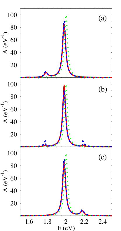
Figure 1: Equilibrium DOS for relatively weak electron-phonon coupling: self-consistent result (solid line), zero-order result (dashed line), uncoupled electron (dotted line). Shown are case of filled (a), partially filled (b), and empty (c) electron level. See text for parameters.

We start by presenting results for the equilibrium density of states $A(E)$. Figure 1 shows results for relatively weak electron-phonon interaction $M_{a}\sim\Gamma$. The parameters used in this calculation are $T=10$ K, $\Gamma_{K}^{(0)}=0.02$ eV ($K=L,R$), $\varepsilon_{0}=2$ eV, $\omega_{0}=0.2$ eV, $M_{a}=0.063$ eV, $\gamma_{ph}=0.001$ eV. This choice corresponds to reorganization energy of $\sim 0.02$ eV, Eq.(7). Results are presented for several choices of Fermi energy position: $E_{F}-\bar{\varepsilon}_{0}=2$ eV (a), $0$ eV (b), and $-2$ eV (c). These cases correspond to filled, partially filled and empty (hole conduction, mixed conduction and electron conduction respectively). The solid line represents the result of a full self-consistent calculation, the dashed line shows the result obtained in the first iteration step (zero-order), and the dotted line shows the DOS $A_{0}$ in the absence of coupling to phonons. First, in all the pictures the polaron shift of the central (elastic) peak position relative to that of $A_{0}$ is evident. Second, due to the low temperature and the relatively weak electron-phonon coupling only one phonon emission peak appears in the plot. This peak is symmetric relative to the electron level position (central peak) for hole and electron transport (compare Fig. 1a and c). In the intermediate regime, Fig. 1b, both satellites appear. In this modest range of electron-phonon interaction the zero-order and the self-consistent results are very close. Note that the zero-order result for filled (Fig. 1a) and empty (Fig. 1c) levels corresponds to single particle transport. In particular, the dashed line in Fig. 1c is exactly the scattering theory result presented in Ref. Wingreen, (see Fig.2a there). Note also that, at least in the low temperature regime, both the scattering theory approach of Wingreen and zero-order approaches within NEGF in the way it is implemented in Lundin ; Balatsky do not describe correctly the hole part of single particle transport.

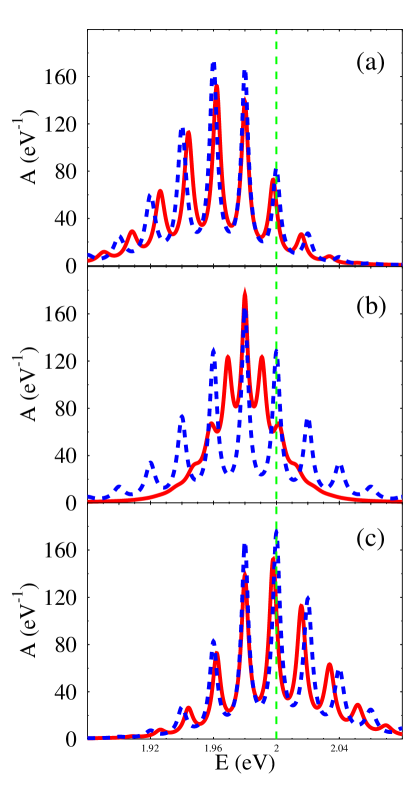
Figure 2: Equilibrium DOS for relatively strong electron-phonon coupling: self-consistent result (solid line) and zero-order result (dashed line). Shown are case of filled (a), partially filled (b), and empty (c) electron level. See text for parameters. Dashed vertical line indicates the position of the DOS peak in the absence of coupling to phonons.

Phonon absorption and emission sidebands are seen at higher temperature and weaker coupling between bridge and leads (Figure 2). The parameters of this calculation are $T=300$ K, $\Gamma_{K}^{(0)}=0.002$ eV ($K=L,R$), $\varepsilon_{0}=2$ eV, $\omega_{0}=0.02$ eV, $M_{a}=0.02$ eV, $\gamma_{ph}=0.001$ eV. The choice corresponds to the same reorganization energy of $\sim 0.02$ eV. However the electron-phonon coupling here is much more pronounced due to weaker coupling to the contacts (which implies that the electron-phonon interaction is relatively much stronger in this case). Once more Fig. 2a is mirror symmetric of Fig. 2c and a polaronic shift of $0.02$ eV between elastic peak in $A$ and $A_{0}$ is observed. The stronger effective electron-phonon coupling is manifested in the appearance of five emission phonon sidebands and three peaks corresponding to absorption and in the fact that the difference between zero-order and self-consistent results is much more pronounced here. Indeed, renormalization due to the interplay between the electron-phonon interaction and the electronic populations in the leads (the Fermi distribution in the contacts influences the phonons which in turn affect the electron energy distribution on the bridge) may change peak heights and positions (see Fig. 2a and c) or even influence the DOS shape drastically (see Fig. 2b). This effect is referred to in Ref. Mitra, as “floating” of the phonon sidebands. The zero-order (dashed) curves in Fig. 2b and c can be compared to the corresponding curves in Fig. 7 of Ref. Kral, . Note that our scheme in zero-order is similar to the NLCE approach of Kral (both approaches utilize a cumulant expansion). However, while the NLCE appears to be problematic when going to the second cluster approximation, our scheme is rather stable when higher order correlations are included by the self-consistent procedure. Moreover, we take the mutual influence of the electron and phonon subsystems into account rather than assuming phonons in thermal equilibrium, as is done in other work Lundin ; Balatsky ; Bratkovsky ; Kral . As was already mentioned, this self-consistent aspect of the calculation may change the results substantially.

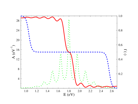
Figure 3: Self-consistent calculation of non-equilibrium DOS (dotted line, left vertical axis) and non-equilibrium electron energy distribution (solid line, right vertical axis). Shown also is the energy distribution for the uncoupled electron (dashed line). See text for parameters.

Figure 3 presents the nonequilibrium DOS (dotted line) and the distribution function (solid line) obtained from the self-consistent calculation. The distribution function in the junction in the absence of coupling to the phonon (dashed line) is shown for comparison. Parameters of the calculation are $T=300$ K, $\Gamma_{K}^{(0)}=0.02$ eV ($K=L,R$), $\varepsilon_{0}=2$ eV, $\omega_{0}=0.2$ eV, $M_{a}=0.2$ eV, $\gamma_{ph}=0.01$ eV (corresponds to reorganization energy of $\sim 0.2$ eV). Voltage drop is $\Phi=1.5$ V with $E_{F}=1.8$ eV and $\mu_{K}=E_{F}\pm\Phi/2$ ($K=L,R$). This setup corresponds to a mixed (both electron and hole) transport through the junction (analog to graph b in Figs. 1 and 2). Local minima in the nonequilibrium population $f$ to the left of the elastic peak (local maxima to the right) correspond to positions of phonon sidebands in the DOS $A$. The effect is due to outscattering of electrons from the energy regions (outscattering of holes from or equivalently inscattering of electrons into the energy regions) due to phonon emission. One sees that strong electron-phonon interaction essentially changes the distribution function. Similar results were reported in Ref. Kral, (see Fig.6 there).

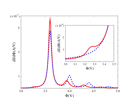
Figure 4: Differential conductance vs. source-drain voltage. Shown are self-consistent (solid line) and zero-order (dashed line) results. Enlarged phonon absorption peak in the self-consistent result is reproduced in the inset. See text for details.

Figure 4 presents self-consistent (solid line) and zero-order (dashed line) results for the differential conductance $dI/d\Phi$ as a function of the applied source-drain voltage $\Phi$. Parameters of the calculation are the same as in Fig. 3 except that the calculation is done at low temperature $T=10$ K. Phonon assisted resonant tunneling reveals itself in conductance peaks associated with different vibronic resonances, i.e. electronic levels dressed by different numbers of phonon excitations. As was mentioned above, renormalization due to electron-phonon interaction leads to shift of position and height of phonon sideband peaks. The zero-order (dashed) curve can be compared to Fig. 6 of Ref. Lundin, . A surprising feature is formation of an additional peak at $\Phi\sim 3.25$ V (see inset) in the self-consistent (solid) curve. While the low temperature of the calculation makes phonon absorption unlikely, we suspect that the effect may be a result of phonon absorption due to heating of the phonon subsystem by electron flux. Clearly such a scenario is possible only if coupling to the contacts is treated beyond second order, i.e. within our scheme only the self-consistent calculation can yield the effect.

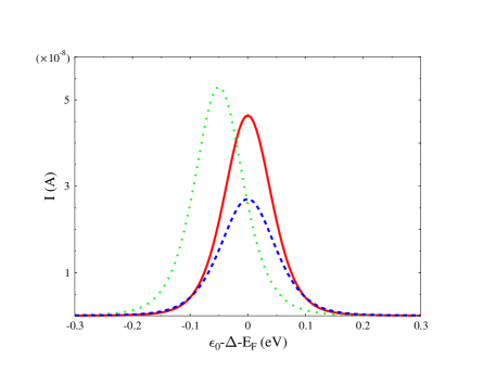
Figure 5: Current vs. gate potential when source-drain voltage is fixed at $\Phi=0.01$ V. The position of the shifted level is given relative to the unbiased Fermi energy. Shown are the self-consistent (solid line), zero-order (dashed line), and uncoupled electron (dotted line) results. See text for details.

Figure 5 presents current plotted against the energy of the bridge electronic level (that can be controlled by a gate voltage) at small fixed source-drain voltage. The horizontal axis represents the position of the shifted electron level relative to the original (unbiased) Fermi energy (average chemical potential of the contacts). Parameters of the calculation are $T=10$ K, $\Gamma_{K}^{(0)}=0.005$ eV ($K=L,R$), $\omega_{0}=0.05$ eV, $M_{a}=0.05$ eV, $\gamma_{ph}=0.001$ eV (corresponds to reorganization energy of $\sim 0.05$ eV). The source-drain voltage drop is $\Phi=0.01$ V. Shown are self-consistent (solid line) and zero-order (dashed line) results. Also shown is current profile when electron and phonon are decoupled (dotted line). The shift in the peak position is due to the reorganization energy.

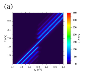
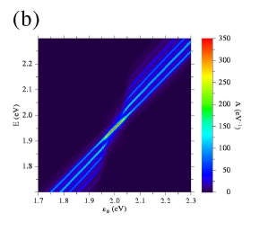
Figure 6: Contour plot of non-equilibrium DOS vs. energy and position of electron level: zero-order (a) and self-consistent (b) results. Parameters of calculation are the same as in Fig. 5.

Mitra et al. Mitra have found that for small source-drain voltage ($\Phi=\Phi_{source}-\Phi_{drain}<\omega_{0}$) no phonon sideband appears in the plot of source-drain current vs. gate voltage potential. This contradicts earlier findings (see Refs. Wingreen, ; Lundin, ; Balatsky, ) and since consideration in Ref. Mitra, is based on the Migdal-Eliashberg theory, which is known to break down in the case of intermediate to strong electron-phonon coupling Mahan ; Hague ; Schonhammer , this finding should be critically examined. The results of Fig. 5 confirm the conclusions of Mitra et al. Note also that the cause of the previous erroneous predictions is neglect or oversimplified description of hole transport FCeh in Wingreen ; Lundin ; Balatsky . Finally, in the case where the couplings to the two contacts are proportional to each other, $\Gamma_{L}(E)=x\Gamma_{R}(E)$, the current through the junction for resonant level model can be obtained as an integral over DOS HaugJauho ; current ,

$$I_{s-d}=\frac{e}{\hbar}\int\frac{dE}{2\pi}\,\frac{\Gamma_{L}(E)\Gamma_{R}(E)}{\Gamma(E)}A(E)\left[f_{L}(E)-f_{R}(E)\right]$$ (45)

In the case of small source-drain voltage, where $\Gamma(E)$ is a smooth function of $E$, the current characteristics are determined by $A(E)$. We can therefore demonstrate the “floating” behavior of phonon sidebands in a contour plot of the DOS vs. energy and electron level position (see Fig. 6). Parameters of the calculation here are the same as in Fig. 5. Figure 6a shows the zero-order result, while Figure 6b presents a self-consistent calculation. One sees that the phonon sidebands disappear around the position of Fermi level $E=E_{F}=1.95$ eV. This in turn leads to absence of peaks in the current lineshape of Fig. 5. Note that since the effect is present already in the zero-order situation (Fig. 6a), it can be studied analytically. We find, that for low temperatures ($T\to 0$) one can not see phonon sidebands in the current-voltage characteristic while changing gate voltage unless $\Phi>\omega_{0}$ (see Appendix E).

V Conclusion

Within a non-equilibrium Green function formalism on the Keldysh contour, we have developed an approximate self-consistent procedure for treating a phonon-assisted resonant level model in the case of intermediate to strong electron-phonon interaction, where the strength of this interaction is determined relative to the bridge-contacts coupling. Our scheme goes beyond earlier considerations of this problem by taking into account the mutual influence of the electron and phonon subsystems. In zero-order and in a single electron transport situation (Fermi energies in the leads far above or far below the bridge level so that the latter is full or empty, respectively) it is similar to other approaches Wingreen ; Lundin ; Balatsky ; Bratkovsky . However in the case of a partially filled resonance level even the zero-order of the self-consistent scheme extends previous calculations (at least in low temperature regime) in treating correctly hole transport. Our approach is also similar in zero-order to the NLCE scheme proposed in Kral , since both use cumulant expansion on the contour. However while NLCE appears to be problematic when going to the second cluster approximation, the present scheme is rather stable when higher order correlations are included by the self-consistent procedure.

We have presented several numerical examples and compared results to those of earlier studies. The self-consistent calculation is found to yield drastically different results as compared to the zero-order theory in the case of strong electron-phonon interaction and in the region of a partially filled electronic level. In particular, it leads to shifts (in position and height) of peaks in the conductance vs. source-drain voltage plot and to phonon absorption signals even at low temperatures, that probably result from heating of the primary phonon by the electronic flux. The non-equilibrium electron DOS and the electron distribution show a similar structure, with peaks associated with phonon emission and absorption. Finally, we confirm the statement of Ref. Mitra, that current measured in a gate voltage experiment, when source-drain voltage is fixed at some small value, will not produce peaks in current vs. position of electron level plot, as was erroneously suggested in Wingreen ; Lundin ; Balatsky . Since the statement in Mitra is based on application of the Migdal-Eliashberg theory, known to break down in the case of intermediate to strong electron-phonon interaction, our confirmation seems to be essential. Together with previous work IETS_SCBA , which deals with the weak electron-phonon interaction case in a self-consistent manner, this provides tools for describing both resonant (intermediate to strong interaction) and off-resonant (weak interaction) tunneling regimes in molecular junctions.

Straightforward generalization of the present scheme would involve retaining mixed terms in deriving the equation of motion for the phonon Green function (Appendix C), thus abandoning the non-crossing approximation (i.e. introducing vertex corrections). One could also go beyond second order in electron-phonon coupling in the cumulant expansion (Appendix B) or in coupling to the contacts in EOMs (Appendices C and D). Development of a scheme spanning the entire range of parameters in the nonequilibrium situation is a goal for future work.

Appendix A Hamiltonian transformation

Here we derive Eq.(6) for the case of weak coupling between the primary phonon and the thermal bath (see below). Let us focus on the part of the Hamiltonian (II) relevant to the electron–phonon interaction

$$\hat{H}_{el-ph} = \varepsilon_{0}\hat{c}^{\dagger}\hat{c}+\omega_{0}\hat{a}^{\dagger}\hat{a}+\sum_{\beta}\omega_{\beta}\hat{b}^{\dagger}_{\beta}\hat{b}_{\beta}$$ (46)

$$+ M_{a}\hat{Q}_{a}\hat{c}^{\dagger}\hat{c}+\sum_{\beta}U_{\beta}\hat{Q}_{a}\hat{Q}_{\beta}$$

We use the small polaron transformation, Eqs. (4) and (5), to get

$$e^{\hat{S}_{a}}\hat{H}_{el-ph}e^{-\hat{S}_{a}}=\left(\varepsilon_{0}-\frac{M_{a}^{2}}{\omega_{0}}\right)\hat{c}^{\dagger}\hat{c}+\omega_{0}\hat{a}^{\dagger}\hat{a}+\sum_{\beta}\omega_{\beta}\hat{b}^{\dagger}_{\beta}\hat{b}_{\beta}$$

$$\quad+\sum_{\beta}U_{\beta}\hat{Q}_{a}\hat{Q}_{\beta}-2\sum_{\beta}M_{a}\frac{U_{\beta}}{\omega_{\beta}}\hat{Q}_{\beta}\hat{c}^{\dagger}\hat{c}$$ (47)

One more transformation

$$e^{\hat{S}_{a}}\hat{H}_{el-ph}e^{-\hat{S}_{a}}\to e^{\hat{S}_{b}}e^{\hat{S}_{a}}\hat{H}_{el-ph}e^{-\hat{S}_{a}}e^{-\hat{S}_{b}}$$ (48)

with

$$\hat{S}_{b}=-2M_{a}\sum_{\beta}\frac{U_{\beta}}{\omega_{0}\omega_{\beta}}\left(\hat{b}^{\dagger}_{\beta}-\hat{b}_{\beta}\right)\hat{c}^{\dagger}\hat{c}$$ (49)

will lead to Hamiltonian $\hat{H}_{el-ph}^{(1)}$ of the form (46) with substitutions

$$\varepsilon_{0}\to\varepsilon_{0}-\Delta^{(1)}\qquad\mbox{and}\qquad M_{a}\to M_{a}^{(1)}$$ (50)

where renormalized parameters are

$$\Delta^{(1)} = \frac{M_{a}^{2}}{\omega_{0}}\left(1+\sum_{\beta}\frac{(2U_{\beta})^{2}}{\omega_{0}\omega_{\beta}}\right)$$ (51)

$$M_{a}^{(1)} = M_{a}\sum_{\beta}\frac{(2U_{\beta})^{2}}{\omega_{0}\omega_{\beta}}$$ (52)

Repeating these transformations a second time leads to a Hamiltonian $\hat{H}_{el-ph}^{(2)}$ of the same form but with different parameters

$$\Delta^{(2)}=\Delta^{(1)}+\frac{\left(M_{a}^{(1)}\right)^{2}}{\omega_{0}}\left(1+\sum_{\beta}\frac{(2U_{\beta})^{2}}{\omega_{0}\omega_{\beta}}\right)$$ (53)

$$=\frac{M_{a}^{2}}{\omega_{0}}\left(1+\sum_{\beta}\left\{\frac{(2U_{\beta})^{2}}{\omega_{0}\omega_{\beta}}+\left[\frac{(2U_{\beta})^{2}}{\omega_{0}\omega_{\beta}}\right]^{2}+\left[\frac{(2U_{\beta})^{2}}{\omega_{0}\omega_{\beta}}\right]^{3}\right\}\right)$$

$$M_{a}^{(2)}=M_{a}^{(1)}\sum_{\beta}\frac{(2U_{\beta})^{2}}{\omega_{0}\omega_{\beta}}=M_{a}\left[\sum_{\beta}\frac{(2U_{\beta})^{2}}{\omega_{0}\omega_{\beta}}\right]^{2}$$ (54)

Repeating the procedure described above, we get for the $n^{th}$ step

$$\Delta^{(n)} = \frac{M_{a}^{2}}{\omega_{0}}\sum_{i=0}^{2n-1}\left[\sum_{\beta}\frac{(2U_{\beta})^{2}}{\omega_{0}\omega_{\beta}}\right]^{i}$$ (55)

$$M_{a}^{(n)} = M_{a}\left[\sum_{\beta}\frac{(2U_{\beta})^{2}}{\omega_{0}\omega_{\beta}}\right]^{n}$$ (56)

Now, assuming that coupling between primary phonon and thermal bath is small in the sense

$$\sum_{\beta}\frac{(2U_{\beta})^{2}}{\omega_{0}\omega_{\beta}}<1$$ (57)

then continuing the procedure in the limit $n\to\infty$ leads to

$$\Delta^{(\infty)} = \frac{M_{a}^{2}}{\omega_{0}}\frac{1}{1-\sum_{\beta}(2U_{\beta})^{2}/\omega_{0}\omega_{\beta}}$$ (58)

$$M_{a}^{(\infty)} = 0$$ (59)

So we arrive at decoupling of electron and phonon degrees of freedom in $\hat{H}_{el-ph}^{(\infty)}$. Going back to the full Hamiltonian (II) of the system we note that the true complete separation of the electronic and phononic degrees of freedom, as achieved in $\hat{H}_{el-ph}^{(\infty)}$, is impossible here due to the coupling between the resonant level and the leads. Instead the aforementioned procedure leads to

$$\hat{H}^{(\infty)} =(\varepsilon_{0}-\Delta^{(\infty)})\hat{c}^{\dagger}\hat{c}+\sum_{k\in\{L,R\}}\varepsilon_{k}\hat{c}_{k}^{\dagger}\hat{c}_{k}$$

$$+\sum_{k\in\{L,R\}}\left(V_{k}\hat{c}_{k}^{\dagger}\hat{c}\hat{X}^{(\infty)}+\mbox{H.c.}\right)$$ (60)

$$+\omega_{0}\hat{a}^{\dagger}\hat{a}+\sum_{\beta}\omega_{\beta}\hat{b}^{\dagger}_{\beta}\hat{b}_{\beta}+\sum_{\beta}U_{\beta}\hat{Q}_{a}\hat{Q}_{\beta}$$

where

$$\hat{X}^{(\infty)} =\hat{X}_{a}^{(\infty)}\hat{X}_{b}^{(\infty)}$$ (61)

$$\hat{X}_{a}^{(\infty)} =\exp\left[-\frac{M_{a}}{\omega_{0}(1-\sum_{\beta}(2U_{\beta})^{2}/\omega_{0}\omega_{\beta})}\left(\hat{a}^{\dagger}-\hat{a}\right)\right]$$ (62)

$$\hat{X}_{b}^{(\infty)} =\prod_{\beta}\exp\left[\frac{M\,2U_{\beta}}{\omega_{0}\omega_{\beta}(1-\sum_{\beta}(2U_{\beta})^{2}/\omega_{0}\omega_{\beta})}\right.$$

$$\qquad\qquad\times\left.\left(\hat{b}^{\dagger}_{\beta}-\hat{b}_{\beta}\right)\right]$$ (63)

Finally, neglecting in the spirit of the non-crossing approximation the $\hat{X}_{b}^{(\infty)}$ operators in the coupling to the contacts, renormalizing $M_{a}$ to incorporate the denominator in the exponent of $\hat{X}_{a}$ expression, and setting $\Delta=\Delta^{(\infty)}$, leads to (6).

Appendix B $<T_{c}\hat{X}(\tau_{1})\hat{X}^{\dagger}(\tau_{2})>$ in terms of $D_{P_{a}P_{a}(\tau_{1},\tau_{2})}$

Here we derive Eq.(17) expressing the shift generator correlation function in terms of the phonon momentum Green function. We start from the Taylor series that expresses the correlation function as a sum of moments

$$<T_{c}\hat{X}(\tau_{1})\hat{X}^{\dagger}(\tau_{2})> =\sum_{n=0}^{\infty}\sum_{m=0}^{\infty}\frac{(-i\lambda_{a})^{n}}{n!}\frac{(i\lambda_{a})^{m}}{m!}$$

$$\times<T_{c}\hat{P_{a}}^{n}(\tau_{1})\hat{P_{a}}^{m}(\tau_{2})>$$ (64)

where Eq. (8) was used. The cumulant expansion for this function is

$$<T_{c}\hat{X}(\tau_{1})\hat{X}^{\dagger}(\tau_{2})>=\exp\left[\sum_{p=1}^{\infty}\frac{\lambda_{a}^{p}}{p!}\varphi_{p}(\tau_{1},\tau_{2})\right]$$

$$\quad=1+\sum_{p=1}^{\infty}\frac{\lambda_{a}^{p}}{p!}\varphi_{p}(\tau_{1},\tau_{2})$$ (65)

$$\quad++\frac{1}{2}\sum_{p_{1}=1}^{\infty}\sum_{p_{2}=1}^{\infty}\frac{\lambda_{a}^{p_{1}}}{p_{1}!}\frac{\lambda_{a}^{p_{2}}}{p_{2}!}\varphi_{p_{1}}(\tau_{1},\tau_{2})\varphi_{p_{2}}(\tau_{1},\tau_{2})+\ldots$$

where $\varphi_{p}(\tau_{1},\tau_{2})$ is a cumulant of order $p$. Considering terms up to $\lambda_{a}^{2}$ and equating same orders of $\lambda_{a}$ in (B) and (B) leads to

$$\left\{\begin{array}[]{l}i<\hat{P}_{a}(\tau_{1})>-i<\hat{P}_{a}(\tau_{2})>=\varphi_{1}(\tau_{1},\tau_{2})\\ 2<T_{c}\hat{P}_{a}(\tau_{1})\hat{P}_{a}(\tau_{2})>-<\hat{P_{a}}^{2}(\tau_{1})>-<\hat{P_{a}}^{2}(\tau_{2})>\\ \quad=\varphi_{2}(\tau_{1},\tau_{2})+{\varphi_{1}}^{2}(\tau_{1},\tau_{2})\end{array}\right.$$ (66)

In steady-state $<\hat{P_{a}}^{n}(\tau_{1})>=<\hat{P_{a}}^{n}(\tau_{2})>=<\hat{P_{a}}^{n}>$, which implies

$$\left\{\begin{array}[]{l}\varphi_{1}(\tau_{1},\tau_{2})=0\\ \varphi_{2}(\tau_{1},\tau_{2})=2<T_{c}\hat{P}_{a}(\tau_{1})\hat{P}_{a}(\tau_{2})>-2<\hat{P_{a}}^{2}>\end{array}\right.$$ (67)

Using this in (B) leads to (17).

Appendix C EOM for $D_{P_{a}P_{a}}(\tau_{1},\tau_{2})$

Here we derive a Dyson-like equation for the phonon momentum Green function $D_{P_{a}P_{a}}$ under the Hamiltonian (6) with the EOM method. Under Hamiltonian (6), the EOM for the shift and momentum operators, Eqs. (2) and (3), in the Heisenberg picture on the Keldysh contour are

$$i\frac{\partial\hat{P}_{a}(\tau)}{\partial\tau} = -i\omega_{0}\hat{Q}_{a}(\tau)-2i\sum_{\beta}U_{\beta}\hat{Q}_{\beta}(\tau)$$ (68)

$$i\frac{\partial\hat{Q}_{a}(\tau)}{\partial\tau} = i\omega_{0}\hat{P}_{a}(\tau)$$

$$- 2\lambda_{a}\sum_{k\in\{L,R\}}\left(V_{k}\hat{c}_{k}^{\dagger}(\tau)\hat{c}(\tau)\hat{X}_{a}(\tau)-\mbox{H.c}\right)$$

$$i\frac{\partial\hat{P}_{\beta}(\tau)}{\partial\tau} = -i\omega_{\beta}\hat{Q}_{\beta}(\tau)-2iU_{\beta}\hat{Q}_{a}(\tau)$$ (70)

$$i\frac{\partial\hat{Q}_{\beta}(\tau)}{\partial\tau} = i\omega_{\beta}\hat{P}_{\beta}(\tau)$$ (71)

We are looking for a Dyson-like equation for the phonon momentum Green function (18). We introduce the operator

$$\hat{D}_{P_{a}P_{a}}^{(0)}{}^{-1}=-\frac{1}{2\omega_{0}}\left[\frac{\partial^{2}}{\partial\tau^{2}}+\omega_{0}^{2}\right]$$ (72)

with property

$$\hat{D}_{P_{a}P_{a}}^{(0)}{}^{-1}\cdot D_{P_{a}P_{a}}^{(0)}(\tau,\tau^{\prime})=D_{P_{a}P_{a}}^{(0)}(\tau,\tau^{\prime})\cdot\hat{D}_{P_{a}P_{a}}^{(0)}{}^{-1}=\delta(\tau,\tau^{\prime})$$ (73)

where $D_{P_{a}P_{a}}^{(0)}$ is the Green function of a free phonon (decoupled both from the electron and the thermal bath). Applying (72) to (18) from the left, taking into account (68)-(71), and restricting consideration to the non-crossing approximation (NCA)Bickers , so that terms mixing different processes are disregarded, one gets

$$\hat{D}_{P_{a}P_{a}}^{(0)}{}^{-1}D_{P_{a}P_{a}}(\tau,\tau^{\prime})=\delta(\tau,\tau^{\prime})+\sum_{\beta}U_{\beta}\frac{\omega_{\beta}}{\omega_{0}}D_{P_{\beta}P_{a}}(\tau,\tau^{\prime})$$

$$+i\lambda_{a}\sum_{k\in\{L,R\}}\left[V_{k}(-i)<T_{c}\hat{c}_{k}^{\dagger}(\tau)\hat{c}(\tau)\hat{X}_{a}(\tau)\hat{P}_{a}(\tau^{\prime})\right.$$ (74)

$$\left.\quad\qquad-V_{k}^{*}(-i)<T_{c}\hat{c}^{\dagger}(\tau)\hat{X}_{a}^{\dagger}(\tau)\hat{c}_{k}(\tau)\hat{P}_{a}(\tau^{\prime})>\right]$$

Next we apply operator (72) to (C) from the right. The procedure is the same in the sense that here we deal once more with EOM for $\hat{P}_{a}$ (the one depending on $\tau^{\prime}$). After tedious but straightforward algebra and convolution of the result with $D_{P_{a}P_{a}}^{(0)}$ we obtain a Dyson-like equation

$$D_{P_{a}P_{a}}(\tau,\tau^{\prime})=D_{P_{a}P_{a}}^{(0)}(\tau,\tau^{\prime})$$ (75)

$$\quad+\int_{c}d\tau_{1}\int_{c}d\tau_{2}\,D_{P_{a}P_{a}}^{(0)}(\tau,\tau_{1})\,\Pi_{P_{a}P_{a}}(\tau_{1},\tau_{2})\,D_{P_{a}P_{a}}^{(0)}(\tau_{2},\tau^{\prime})$$

with the self-energy expression

$$\Pi_{P_{a}P_{a}}(\tau_{1},\tau_{2})=\sum_{\beta}\frac{2U_{\beta}^{2}\omega_{\beta}}{\omega_{0}^{2}}\delta(\tau_{1},\tau_{2})$$ (76)

$$+\sum_{\beta}\left(U_{\beta}\frac{\omega_{\beta}}{\omega_{0}}\right)^{2}D_{P_{\beta}P_{\beta}}(\tau_{1},\tau_{2})-i\lambda_{a}^{2}\sum_{k\in\{L,R\}}|V_{k}|^{2}$$

$$\times\left[g_{k}(\tau_{2},\tau_{1})G_{c}^{(0)}(\tau_{1},\tau_{2})<T_{c}\hat{X}_{a}(\tau_{1})\hat{X}_{a}^{\dagger}(\tau_{2})>_{0}+\mbox{H.c.}\right]$$

In what follows we neglect renormalization of the phonon frequency due to coupling to the thermal bath (first term on the right and real part of the second term in the self-energy expression). This is in analogy to the wide band approximation (for discussion on applicability of the approximation to coupling to the thermal bath case see Ref. IETS_SCBA, ). In the second term on the right we also replace $\omega_{\beta}/\omega_{0}$ by unity arguing that main contribution to $D_{P_{a}P_{a}}$ comes from the region $\omega_{\beta}\sim\omega_{0}$. Then the dressed form (zero-order Green and correlation functions are substituted by the full ones) of (76) is Eq.(II).

Appendix D EOM for $G_{c}(\tau_{1},\tau_{2})$

Here we derive a Dyson-like equation for electron Green function $G_{c}$ under Hamiltonian (6) using the EOM method. First we note that under Hamiltonian (6), the EOM for operator $\hat{c}$ in the Heisenberg picture on the Keldysh contour is

$$i\frac{\partial\hat{c}(\tau)}{\partial\tau}=\bar{\varepsilon}_{0}\hat{c}(\tau)+\sum_{k\in\{L,R\}}V_{k}^{*}\hat{X}_{a}^{\dagger}(\tau)\hat{c}_{k}(\tau)$$ (77)

with the corresponding Hermitian conjugate for the creation operator $\hat{c}^{\dagger}$. We then introduce the operator

$$\hat{G}_{c}^{(0)}{}^{-1}=i\frac{\partial}{\partial\tau}-\bar{\varepsilon}_{0}$$ (78)

with the property

$$\hat{G}_{c}^{(0)}{}^{-1}\cdot G_{c}^{(0)}(\tau,\tau^{\prime})=G_{c}^{(0)}(\tau,\tau^{\prime})\cdot\hat{G}_{c}^{(0)}{}^{-1}=\delta(\tau,\tau^{\prime})$$ (79)

Here $G_{c}^{(0)}(\tau,\tau^{\prime})$ is the Green function for an electronic level decoupled from the contacts. Applying it to the electron Green function $G_{c}(\tau,\tau^{\prime})$ first from the left and then from the right, one gets

$$\hat{G}_{c}^{(0)}{}^{-1}\cdot G_{c}(\tau,\tau^{\prime})\cdot\hat{G}_{c}^{(0)}{}^{-1}=\delta(\tau,\tau^{\prime})\cdot\hat{G}_{c}^{(0)}{}^{-1}$$ (80)

$$\quad+\sum_{k\in\{L,R\}}|V_{k}|^{2}g_{k}(\tau,\tau^{\prime})<T_{c}\hat{X}_{a}(\tau^{\prime})\hat{X}_{a}^{\dagger}(\tau)>$$

Finally, we take convolution of (80) with $G_{c}^{(0)}$ from left and right and utilize Eq.(79) to arrive at a Dyson-like equation for $G_{c}$ with the dressed self-energy of the form presented in (22).

Appendix E Phonon sidebands in current-voltage characteristics

Here we study analytically the possibility of observing phonon sidebands in current-voltage characteristics when the gate voltage applied to the junction is varied. We restrict our consideration to the zero-order situation (first step of the self-consistent procedure) and low temperature (we take $T=0$). The zero-order correlation functions for the shift generator operators (in the time domain) are

$$<\hat{X}_{a}(t)\hat{X}^{\dagger}_{a}(0)>$$ (81)

$$=e^{-\lambda_{a}^{2}(2N_{0}+1)}\exp\{\lambda_{a}^{2}[(N_{0}+1)e^{-i\omega_{0}t}+N_{0}e^{i\omega_{0}t}]\}$$

$$\stackrel{{\scriptstyle T\to 0}}{{\longrightarrow}}e^{-\lambda_{a}^{2}}\exp\{\lambda_{a}^{2}e^{-i\omega_{0}t}\}\equiv e^{-\lambda_{a}^{2}}\sum_{k=0}^{\infty}\frac{\lambda_{a}^{2k}}{k!}e^{-ik\omega_{0}t}$$

$$<\hat{X}^{\dagger}_{a}(0)\hat{X}_{a}(t)>$$ (82)

$$=e^{-\lambda_{a}^{2}(2N_{0}+1)}\exp\{\lambda_{a}^{2}[N_{0}e^{-i\omega_{0}t}+(N_{0}+1)e^{i\omega_{0}t}]\}$$

$$\stackrel{{\scriptstyle T\to 0}}{{\longrightarrow}}e^{-\lambda_{a}^{2}}\exp\{\lambda_{a}^{2}e^{i\omega_{0}t}\}\equiv e^{-\lambda_{a}^{2}}\sum_{k=0}^{\infty}\frac{\lambda_{a}^{2k}}{k!}e^{ik\omega_{0}t}$$

Within the wide-band approximation, the zero-order lesser and greater electron Green functions (in the energy domain) are

$$G_{c}^{<}(E) = \frac{i\theta(\mu_{L}-E)\Gamma_{L}+i\theta(\mu_{R}-E)\Gamma_{R}}{(E-\bar{\varepsilon}_{0})^{2}+(\Gamma/2)^{2}}$$ (83)

$$G_{c}^{>}(E) = \frac{-i\theta(E-\mu_{L})\Gamma_{L}-i\theta(E-\mu_{R})\Gamma_{R}}{(E-\bar{\varepsilon}_{0})^{2}+(\Gamma/2)^{2}}$$ (84)

Applying (81)-(84) to (14), using the resulting Green function in (43) and the spectral function $A$ in (45) leads to an expression for the source-drain current in the form (putting $\mu_{L}-\mu_{R}=\Phi>0$)

$$I_{sd} = \frac{e}{\hbar}\frac{\Gamma_{L}\Gamma_{R}}{\Gamma}e^{-\lambda_{a}^{2}}\sum_{k=0}^{\infty}\frac{\lambda_{a}^{2k}}{k!}$$

$$\times \int_{\mu_{R}}^{\mu_{L}}\frac{dE}{2\pi}\left[\frac{\theta(E-k\omega_{0}-\mu_{R})\Gamma_{R}}{(E-k\omega_{0}-\bar{\varepsilon}_{0})^{2}+(\Gamma/2)^{2}}\right.$$

$$\qquad\qquad\left.+\frac{\theta(\mu_{L}-E-k\omega_{0})\Gamma_{L}}{(E+k\omega_{0}-\bar{\varepsilon}_{0})^{2}+(\Gamma/2)^{2}}\right]$$

while the gate voltage changes the position of $\bar{\varepsilon}_{0}$. It is obvious that one can not observe phonon sidebands ($k>0$ terms) in the source-drain current-voltage unless $\Phi>\omega_{0}$.

References

-
(1)
Molecular Electronics II, Eds. A. Aviram, M. Ratner,
V. Mujica, Ann. N.Y. Acad. Sci., vol. 960 (2002);
Molecular Electronics III, Eds. J. R. Reimers, C. A. Picconatto, J. C. Ellenbogen, R. Shashidhar, Ann. N.Y. Acad. Sci., vol. 1006 (2003). - (2) A. Nitzan, Ann. Rev. Phys. Chem. 53, 681 (2001).
- (3) Molecular Nanoelectronics, Eds. M. A. Reed and T. Lee, American Scientific Publishers (2003).
- (4) D. R. Bowler, J. Phys.: Condens. Matter 16, R721 (2004).
- (5) H. Park, J. Park, A. K. L. Lim, E. H. Anderson, A. P. Alivisatos, and P. L. McEuen, Nature 407, 57 (2000).
-
(6)
J. Gaudioso, L. J. Lauhon, and W. Ho,
Phys. Rev. Lett. 85, 1918 (2000);
X. H. Qiu, G. V. Nazin, and W. Ho, Phys. Rev. Lett. 93, 196806 (2004). -
(7)
B. C. Stipe, M. A. Rezaei, and W. Ho,
Rev. Sci. Instruments 70, 137 (1999);
Phys. Rev. Lett. 82, 1724 (1999);
J. R. Hahn, H. J. Lee, and W. Ho, Phys. Rev. Lett. 85, 1914 (2000);
X. H. Qiu, G. V. Nazin, and W. Ho, Phys. Rev. Lett. 92, 206102 (2004). - (8) N. B. Zhitenev, H. Meng, and Z. Bao, Phys. Rev. Lett. 88, 226801 (2002).
- (9) E. M. Weig, R. H. Blick, T. Brandes, J. Kirschbaum, W. Wegscheider, M. Bichler, and J. P. Kotthaus, Phys. Rev. Lett. 92, 046804 (2004).
- (10) L. H. Yu, Z. K. Keane, J. W. Ciszek, L. Cheng, M. P. Stewart, J. M. Tour, and D. Natelson, Phys. Rev. Lett. 93, 266802 (2004).
- (11) R. H. M. Smit, C. Untiedt, and J. M. van Ruitenbeek, Nanotechnology 15, S472 (2004).
-
(12)
W. Wang, T. Lee, and M. A. Reed,
Rep. Prog. Phys. 68, 523 (2005);
J. Phys. Chem. B 108, 18398 (2004);
W. Wang, T. Lee, I. Kretschmar, and M. A. Reed, Nano Lett. 4, 643 (2004). -
(13)
J. G. Kushmerick, D. L. Allara, T. E. Mallouk, and
T. S. Mayer, MRS Bulletin 29, 396 (2004);
J. G. Kushmerick, J. Lazorcik, C. H. Patterson, R. Shashidhar, D. S. Seferos, and G. C. Bazan, Nano Lett. 4, 639 (2004). - (14) Y. Selzer, M. A. Cabassi, T. S. Mayer, and D. L. Allara, Nanotechnology 15, S483 (2004).
- (15) N. A. Pradhan, N. Liu, and W. Ho, J. Phys. Chem. B 109, 8513 (2005).
- (16) G. D. Mahan, Many-Particle Physics. (Third edition, Kluwer Academic/Plenum Publishers, New York, 2000).
- (17) Y.-C. Chen, M. Zwolak, and M. Di Ventra, Nano Lett. 3, 1691 (2003); Nano Lett. 4, 1709 (2004); cond-mat/0412511 (2004).
-
(18)
T. N. Todorov,
Phil. Mag. B 77, 965 (1998);
M. J. Montgomery, T. N. Todorov, and A. P. Sutton, J. Phys.: Cond. Mat. 14, 5377 (2002);
M. J. Montgomery, J. Hoekstra, T. N. Todorov, and A. P. Sutton, J. Phys.: Cond. Mat. 15, 731 (2003);
M. J. Montgomery and T. N. Todorov, J. Phys.: Cond. Mat. 15, 8781 (2003). -
(19)
S. Alavi and T. Seideman,
J. Chem. Phys. 115, 1882 (2001);
S. Alavi, B. Larade, J. Taylor, H. Guo, and T. Seideman, Chem. Phys. 281, 293 (2002). -
(20)
H. Ness and A. J. Fisher,
Phys. Rev. Lett. 83, 452 (1999);
cond-mat/0201276 (2002);
Chem. Phys. 281, 279 (2002);
Eur. Phys. J. D 24, 409 (2003);
H. Ness, S. A. Shevlin, and A. J. Fisher, Phys. Rev. B 63, 125422 (2001); -
(21)
K. Haule and J. Bonča,
Phys. Rev. B 59, 13087 (1999);
J. Bonča and S. A. Trugman, Phys. Rev. Lett. 75, 2566 (1995). -
(22)
A. Troisi, M. A. Ratner, and A. Nitzan,
J. Chem. Phys. 118, 6072 (2003);
A. Troisi, A. Nitzan, and M. A. Ratner, J. Chem. Phys. 119, 5782 (2003). - (23) L. V. Keldysh, Sov Phys. JETP 20, 1018 (1965).
-
(24)
S. Datta, Electronic Transport in Mesoscopic Systems,
Cambridge University Press (1997);
S. Datta, Quantum Transport: Atom to Transistor, Cambridge University Press (2005). - (25) H. Haug and A.-P. Jauho, Quantum Kinetics in Transport and Optics of Semiconductors. (Springer, Berlin, 1996).
- (26) A. Nitzan, J. Jortner, J. Wilkie, A. L. Burin, and M. A. Ratner, J. Phys. Chem. B 104, 5661 (2000).
- (27) A. Bayman, P. K. Hansma, and W. C. Kaska, Phys. Rev. B 24, 2449 (1981).
-
(28)
A. B. Migdal, Soviet Physics JETP 7, 996 (1958);
G. M. Eliashberg, Soviet Physics JETP 11, 696 (1960). - (29) A. L. Fetter and J. D. Walecka, Quantum Theory of Many-Particle Systems. (Dover Publications, Inc., Mineola and New York, 2003).
- (30) C. H. Grein, E. Runge, and H. Ehrenreich, Phys. Rev. B 47, 12590 (1993).
- (31) P. Hyldgaard, S. Hershfield, J. H. Davies, and J. W. Wilkins, Ann. Phys. 236, 1 (1994).
-
(32)
S. Datta,
J. Phys.: Cond. Mat. 2, 8023 (1990);
R. Lake and S. Datta, Phys. Rev. B 45, 6670 (1992); 46, 4757 (1992). -
(33)
S. G. Tikhodeev, M. Natario, K. Makoshi, T. Mii, and H. Ueba,
Surf. Sci. 493, 63 (2001);
T. Mii, S. G. Tikhodeev, and H. Ueba, Surf. Sci. 502–503, 26 (2002); Phys. Rev. B 68, 205406 (2003). - (34) A. Pecchia, A. Di Carlo, A. Gagliardi, S. Sanna, T. Frauenheim, and R. Gutierrez, Nano Lett. 4, 2109 (2004).
- (35) A. Mitra, I. Aleiner, and A. J. Millis, Phys. Rev. B 69, 245302 (2004).
- (36) T. Yamamoto, K. Watanabe, and S. Watanabe, Phys. Rev. Lett. 95, 065501 (2005).
- (37) M. Galperin, M. A. Ratner, and A. Nitzan, J. Chem. Phys. 121, 11965 (2004); Nano Lett. 4, 1605 (2004).
- (38) D. A. Ryndyk and J. Keller, Phys. Rev. B 71, 073305 (2005).
- (39) H. Park, J. Park, A. K. L. Lim, E. H. Anderson, A. P. Alivisatos, and P. L. McEuen, Nature 407, 57 (2000).
- (40) J. Park, A. N. Pasupathy, J. I. Goldsmith, C. Chang, Y. Yaish, J. R. Petta, M. Rinkoski, J. P. Sethna, H. D. Abruña, P. L. McEuen, and D. C. Ralph, Nature 417, 722 (2002).
- (41) L. H. Yu and D. Natelson, Nano Lett. 4, 79 (2004).
- (42) N. S. Wingreen, K. W. Jacobsen, and J. W. Wilkins, Phys. Rev. B 40, 11834 (1989).
- (43) U. Lundin and R. H. McKenzie, Phys. Rev. B 66, 075303 (2002).
- (44) J.-X. Zhu and A. V. Balatsky, Phys. Rev. B 67, 165326 (2003).
- (45) A. S. Alexandrov, A. M. Bratkovsky, and R. S. Williams, Phys. Rev. B 67, 075301 (2003); A. S. Alexandrov and A. M. Bratkovsky, Phys. Rev. B 67, 235312 (2003).
- (46) P. Král, Phys. Rev. B 56, 7293 (1997).
- (47) S. Braig and K. Flensberg, Phys. Rev. B 68, 205324 (2003).
- (48) J. Koch and F. von Oppen, Phys. Rev. Lett. 94, 206804 (2005); J. Koch, M. Semmelhack, F. von Oppen, and A. Nitzan, cond-mat/0504095 (2005).
- (49) K. Flensberg, Phys. Rev. B 68, 205323 (2003).
- (50) P. S. Cornaglia, H. Ness, and D. R. Grempel, Phys. Rev. Lett. 93, 147201 (2004); P. S. Cornaglia, D. R. Grempel, and H. Ness, Phys. Rev. B 71, 075320 (2005); P. S. Cornaglia and D. R. Grempel, Phys. Rev. B 71, 245326 (2005).
- (51) I. G. Lang and Yu. A. Firsov, Sov. Phys. JETP 16, 1301 (1963).
- (52) N. E. Bickers, Rev. Mod. Phys. 59, 845 (1987).
- (53) Y. Meir and N. S. Wingreen, Phys. Rev. Lett. 68, 2512 (1992); A. P. Jauho, N. S. Wingreen, and Y. Meir, Phys. Rev. B 50, 5528 (1994).
- (54) M. K. Grover and R. Silbey, J. Chem. Phys. 52, 2099 (1970).
- (55) D. C. Langreth, Linear and Nonlinear Response Theory with Applications, p. 3–32 in: Linear and Nonlinear Electron Transport in Solids, Eds. J. T. Devreese and D. E. Doren (Plenum Press, New York and London, 1976).
- (56) Note that . Both appear in (34) and (35) in order to demonstrate the projection rule: if on the contour, then .
- (57) J. P. Hague and N. d’Ambrumenil, cond-mat/0106355 (2001).
- (58) V. Meden, K. Schönhammer, and O. Gunnarsson, Phys. Rev. B 50, 11179 (1994).
- (59) The Franck-Condon factor for electron and hole transport is different: for electrons and for holes. Refs. Wingreen, ; Lundin, ; Balatsky, take it in the same (electron-type) form for both types of transport, and this is the main cause of consequent erroneous predictions.