UNIVERSITÀ DEGLI STUDI DI ROMA “LA SAPIENZA”

FACOLTÀ DI SCIENZE MATEMATICHE, FISICHE E NATURALI

Dottorato in Fisica - Ph. D. in Physics
XVIII ciclo

Some applications of recent theories
of disordered systems

Supervisors: Candidate:

Prof. Giorgio Parisi Dr. Francesco Zamponi
Prof. Giancarlo Ruocco

October, 2005

Introduction

This Ph.D. thesis is divided in two parts. The first one concerns the equilibrium properties of glassy systems, i.e. properties that can be derived from the Gibbs distribution. Non–glassy equilibrium systems are very well understood. Many different thermodynamic phases of classical many-body systems are known and their properties can be computed starting from the Gibbs distributions or its decomposition in pure states. Quantum effects can be taken into account leading to new thermodynamic phases (superfluids, or superconductors) whose statistical properties are also well understood. The phase transitions between different phases have been extensively studied in the last century and their current understanding is very satisfactory.

The theoretical understanding of the glass phase and the related glass transition, on the contrary, is still poor, even if many important progresses have been recently achieved. Despite the existence of a number of mean field models which reproduce the basic phenomenology of glassy systems, and for which the glass transition can be fully characterized, the existence of a thermodynamic glass transition in finite dimension is still a matter of debate. Many authors believe that the glass transition in finite dimension is a purely dynamical phenomenon that cannot be derived from the Gibbs distribution. The situation is complicated by the absence of a simple finite dimensional glassy model which could play, in the context of glassy systems, the role that the Ising model played in the context of second order phase transitions. Experiments and numerical simulations can only investigate the nonequilibrium counterpart of the (eventual) thermodynamical glass transition, so experimental data on pure thermodynamical glassy states are not available. Thus, the problem of the existence of a thermodynamic glass transition in finite dimension, and many related problems, such as the existence of a diverging correlation length, can only be addressed by analytical solution, either exact or approximate, of “glassy” models.

Mean field models are - up to now - the only solvable models of glassy systems: they provide an useful framework to describe the basic phenomenology observed in experiments. Their detailed investigation revealed that the glass transition is connected with the existence of an exponential number (in the size of the system) of metastable states. The characterization of these metastable states allowed to understand their relevance for the dynamics of the system: it emerged that they play a key role in the nonequilibrium dynamics of glasses and are responsible for the existence of a nonequilibrium glass transition which closely reflects the one that is observed in real glassy materials.

Some aspects of the phenomenology of glasses and a theory attempting to describe them are presented in chapter 1. As an example of simple model for the glass transition in finite dimension, I studied the Hard Sphere liquid (in collaboration with G. Parisi). This study is presented in chapter 2. Obviously the model is not exactly solvable, but it was possible to solve it approximately by means of a replica trick and of the HNC approximation - a standard approximation in the theory of simple liquids. This strategy was already successfully applied by M. Mézard and G. Parisi to analytic potentials (e.g. Lennard-Jones), but the application to Hard Spheres required some additional work due to the singularity of the interaction potential. In this approximation, a thermodynamic glass transition is found. The equation of state of the glass and its pair correlation function $g(r)$ can be computed. This allows also to obtain an estimate of the random close packing density and of the mean coordination number in the amorphous packings. The results agree well with the available numerical data and with other theories. This is encouraging but does not solve the problem of the existence of the glass transition in finite dimension because of the approximations involved.

As discussed above mean field models reproduce many aspects of the phenomenology of glasses. In chapter 3 it is shown (in collaboration with G. Parisi and G. Ruocco) that these models also reproduce a correlation between the fragility of a liquid - to be defined in chapter 1 - and the vibrational properties of its glass that has been recently found by T. Scopigno et al. analyzing experimental data on a wide class of glassy materials. This result is - in our opinion - an interesting confirmation of the relevance of mean field models in the description of the phenomenology of real glasses. An outcome of this study is that the number of metastable states is a decreasing function of fragility; this prediction differs from the one that has been obtained by other authors and can be tested, in principle, on real materials.

The second part of the thesis concerns some recent attempts - discussed in chapter 4 - to build a statistical theory of nonequilibrium stationary states induced by the application of an external driving force on a thermostatted system. From the chaotic hypothesis, an extension of the ergodic hypothesis to nonequilibrium systems proposed by E. G. D. Cohen and G. Gallavotti, an explicit expression for the measure describing the system in stationary state can be derived. For time-reversible systems, an interesting prediction of this theory is the validity of the fluctuation relation: a relation between the probability of positive and negative large fluctuations of the phase space contraction rate $\sigma$, often identified with the entropy production rate. What is remarkable is that the fluctuation relation is universal, in the sense that it contains no model-dependent parameters.

A test of the fluctuation relation is then a rather stringent test of the theory, and indeed it has been performed in a number of cases, in the last decade, with positive result. In chapter 5 (in collaboration with A. Giuliani and G. Gallavotti) the fluctuation relation is tested in a numerical simulation of a system of particles interacting via a Lennard-Jones–like potential and subjected to an external driving force and to a thermostatting force (isokinetic constraint). With respect to previous studies of similar systems, an important progress has been obtained: the observation of non-Gaussian tails in the probability distribution of $\sigma$. This is important because the fluctuation relation is related to the Green-Kubo relations at the Gaussian level, so a test that is really independent from linear response theory requires the observation of non-Gaussian tails. This progress was possible thanks to the increase of computational power in the last years.

In chapter 6 some aspects of the driven nonequilibrium dynamics of glassy systems are discussed. In the limit of small driving force (small entropy production), it has been shown by L. Cugliandolo and J. Kurchan that a nonequilibrium effective temperature can be introduced, which has the property of being a temperature in the thermodynamic sense: it controls heat flows and enters the relation between spontaneous fluctuations and response to external perturbations as in equilibrium. The systems reaches a stationary state and it is possible to decompose the dynamics in different time scales. On each time scale, a single effective temperature is defined. The system behaves as if composed by many non-interacting subsystems, evolving on well separated time scales, each one characterized by the corresponding effective temperature.

The fluctuation relation is related to the definition of temperature out of equilibrium. For driven systems evolving on a single time scale and in contact with an equilibrated bath at temperature $T$, the temperature of the bath controls the fluctuations of the entropy production rate. Thus, one can ask if, for driven glasses, a modified fluctuation relation can be introduced, in which the effective temperature enters instead of the temperature of the bath. This idea was first investigated by M. Sellitto, and many proposals in this direction subsequently appeared. I investigated (in collaboration with F. Bonetto, L. Cugliandolo and J. Kurchan) a very simple model for glassy dynamics: a Brownian particle in contact with a bath whose correlation and response function do not satisfy the fluctuation–dissipation relation. An effective temperature can be defined, and we showed that a modified fluctuation relation holds, in which the temperature of the bath is replaced by the effective temperature. These results are presented in chapter 7 where they are also compared with similar results that recently appeared in the literature. Some numerical data, obtained on a sheared Lennard-Jones–like system in the glassy regime (in collaboration with L. Angelani and G. Ruocco), are also presented. They partially confirm the results obtained analytically. Unfortunately, a numerical check of all the predictions of the model is impossible because the time scales involved are beyond the ones accessible to the numerical simulation.

Chapters 1, 4 and 6 are introductory chapters, while in chapters 2, 3, 5 and 7 original results are presented. It is important to remark that this is not a review article. In the introductory chapters, I made no attempt to quote all the theories, numerical data, experimental results avalaible on the subject. For example, in chapter 1 the inherent structures approach is missing, and in chapter 6 only the dynamics of mean field models is discussed, without any attempt to review the rich dynamical phenomenology of real materials and the theories attempting to describe it (e.g. Mode-Coupling theories). Only the notions that were needed to present the original results have been included in the introductory chapters. This does not necessarily mean that I prefer the theories presented in these chapters to other ones.

The results collected here have been published in:

• Chapter 2: G. Parisi and F. Zamponi, J. Chem. Phys. 123, 144501 (2005).

• Chapter 3: G. Parisi, G. Ruocco and F. Zamponi, Phys. Rev. E 69, 061505 (2004).

• Chapter 5: A. Giuliani, F. Zamponi and G. Gallavotti, J. Stat. Phys. 119, 909 (2005).

• Chapter 7: F. Zamponi, G. Ruocco and L. Angelani, Phys. Rev. E 71, 020101(R) (2005);
   F. Zamponi, F. Bonetto, L. Cugliandolo and J. Kurchan, J. Stat. Mech. (2005) P09013.

Part I Equilibrium

Chapter 1 The glass transition

1.1 Basic phenomenology

Although liquids normally crystallize on cooling, there are members of all liquids types (including molecular, ionic and metallic) that can be supercooled below the melting temperature $T_{m}$ and then solidify at some temperature $T_{g}$, the glass transition temperature. The viscosity $\eta(T)$ of the liquid increases continuously but very fast below $T_{m}$ and at some point reaches values so high that the liquid does not flow anymore and can be considered a solid for all practical purposes: at low temperatures, an amorphous solid phase is observed. The temperature $T_{g}$ marking the transition between the liquid and the glass is often defined by the condition $\eta(T_{g})=10^{13}$ Poise, but many other definitions are possible.

As an example of this phenomenon, in Fig. 1.1 the viscosity of many glass forming liquids is reported as a function of the temperature. Following Angell [1, 2, 3], the quantity $\log_{10}\left[\frac{\eta(T)}{\rm Poise}\right]$ is reported as a function of $T_{g}/T$. The viscosity increases of about $17$ orders of magnitude on decreasing the temperature by a factor $2$. Note that as the increase of viscosity is so fast, the dependence of $T_{g}$ on the particular value of viscosity ($10^{13}$ Poise) which is chosen to define it is very weak.

It is often found that the viscosity around $T_{g}$ follows the Vogel–Fulcher–Tamman (VFT) law [4],

$$\eta(T)=\eta_{\infty}e^{\frac{\Delta}{T-T_{0}}}\ ,$$ (1.1)

where $\eta_{\infty}$, $\Delta$ and $T_{0}$ are system–dependent parameters. If $T_{0}=0$ this relation reduces to the Arrhenius law; otherwise, the extrapolation of the viscosity below $T_{g}$ leads to a divergence at $T=T_{0}$.

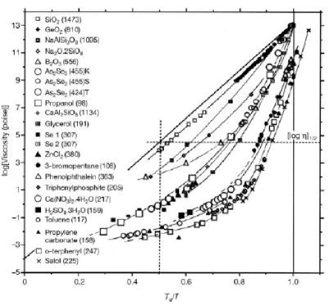
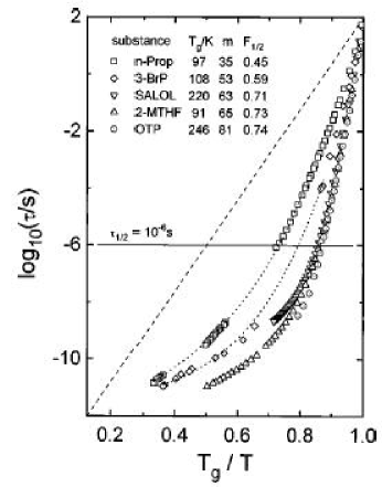
Figure 1.1: (Left, from [3]) Viscosity data for many glass forming liquids. The logarithm of the viscosity measured in Poise is reported as a function of $T_{g}/T$. The (calorimetric) $T_{g}$ is defined as the temperature at which the enthalpy relaxation time is $\sim 200$s, and its value is reported in parenthesis in the key of the figure. Note that for some systems the value of the calorimetric $T_{g}$ does not satisfy exactly the condition $\eta(T_{g})=10^{13}$ Poise. Fragility is the slope of the curves in $T_{g}/T=1$. (Right, from [6]) Structural relaxation time obtained from dielectric relaxation measurements. The dashed line indicates Arrhenius behavior. The value of $T_{g}$, obtained from $\tau_{\alpha}(T_{g})=100$s, and of fragility are reported in the key.

1.1.1 Fragility

The fragility concept has been introduced by Angell [5]. It describes how fast the viscosity increases with decreasing temperature on approaching $T_{g}$. “Strong” glasses (low values of fragility) show a “weak” $T$ dependence of $\eta(T)$, which is often described by the Arrhenius law (see e.g. the curve for ${\rm SiO}_{2}$ in Fig. 1.1), while “fragile” glasses show a much faster $T$ dependence of the relaxation time, often described by the VFT law with $T_{0}\neq 0$. A common example of fragile glass former is the o-terphenyl (OTP), see Fig. 1.1.

If the VFT law holds, the ratio $\frac{T_{g}}{T_{g}-T_{0}}$ can be taken as a fragility index: it ranges from $1$ for strong glasses to $\sim 10$ for the most fragile glasses [2]. However, the common definition of the fragility index, which is also independent of the VFT law, is

$$m_{A}\equiv\left.\frac{d\log_{10}\left[\frac{\eta(T)}{\rm Poise}\right]}{d(T_{g}/T)}\right|_{T=T_{g}}\ ,$$ (1.2)

i.e. it is given by the slope of the curves in Fig. 1.1 at $T_{g}/T=1$. This definition involves only the derivative of the viscosity at $T_{g}$, without any assumption on the global behavior of $\eta(T)$. According to this definition, a strong glass (strictly Arrhenius behavior) would have $m_{A}\sim 17$ (being $\eta_{\infty}=10^{-4}$ Poise and $\eta(T_{g})=10^{13}$ Poise), while the most fragile systems reach $m_{A}\sim 160$ [2]. If the VFT law holds it is easy to show that $m_{A}\sim\frac{17T_{g}}{T_{g}-T_{0}}$.

1.1.2 Structural relaxation time

The viscosity is related to the structural relaxation time $\tau_{\alpha}$ by the Maxwell relation, $\eta=G_{\infty}\tau_{a}$, where $G_{\infty}$ is the infinite–frequency shear modulus of the liquid. The structural relaxation time is related to the decorrelation of density fluctuations. In glass forming liquids, for $T_{m}\gg T\geq T_{g}$, the decorrelation of density fluctuations happens on two well separated time scales: a “fast” time scale ($\sim 10^{-12}s$), which is related to vibrations of the particles around the disordered instantaneous positions, and a “slow” time scale $\tau_{\alpha}$, which is related to cooperative rearrangements of the disordered structure around which the fast vibrations take place. Through the Maxwell relation, the fast increase of viscosity around $T_{g}$ is then related to a marked slowing down of the structural dynamics; usually, at $T_{g}$ one has $\tau_{\alpha}\sim 100s$, while in the liquid phase $\tau_{\alpha}\sim\mu s$.

The structural relaxation time, obtained from dielectric relaxation data, of some fragile glass forming liquids is reported in the right panel of Fig. 1.1. The behavior of $\tau_{\alpha}(T)$ is also described by a VFT law with an apparent divergence at $T=T_{0}$. This leads to the interpretation of $T_{0}$ as a temperature at which a structural arrest takes place.

A common pictorial interpretation of the dynamics of glass forming liquids above $T_{g}$ is the following: for short times the particles are “caged” by their neighbors and vibrate around a local structure on a nanometric scale; the structural relaxation is then interpreted as a slow cooperative rearrangement of the cages. Note that on the time scale of the structural relaxation time $\tau_{\alpha}$, the mean square displacement of the particles is smaller than the particle radius, so one cannot think to the structural relaxation as a process of single–particle “jumps” between adjacent cages.

1.1.3 Configurational (or excess) entropy

The idea that the dynamics in the supercooled phase is separated in a fast intra–cage motion and in a slow cooperative rearrangement of the structure suggests to split the total entropy of the liquid in a “vibrational” contribution, related to the volume of the cages, and a “configurational” contribution, that counts the number of different disordered structures that the liquid can assume [7]:

$$S_{liq}(T)\sim S_{vib}(T)+S_{c}(T)\ .$$ (1.3)

To estimate the vibrational contribution to the entropy of the liquid, one can assume that it is roughly of the order of the entropy of the corresponding crystal. It is then possible to estimate $S_{c}(T)$ as

$$S_{c}(T)=S_{liq}(T)-S_{cryst}(T)=\Delta S_{m}-\int_{T}^{T_{m}}d\log T^{\prime}\,\big{[}C_{liq}(T^{\prime})-C_{cryst}(T^{\prime})\big{]}\ ,$$ (1.4)

where $\Delta S_{m}\equiv S_{liq}(T_{m})-S_{cryst}(T_{m})$ is the entropy difference between the liquid and the crystal at the melting temperature $T_{m}$, and $C(T)=T\frac{\partial S}{\partial T}$ is the specific heat. Note that in experiments one usually works at constant pressure, $C=C_{p}$, while in numerical simulations and in theoretical computations one usually works at constant volume, $C=C_{v}$. The configurational entropy $S_{c}$ is sometimes called “excess entropy”.

In Fig. 1.2 the estimate of $S_{c}$, obtained from calorimetric measurements of the specific heat and using Eq. (1.4), is reported for four different fragile glass formers. Below $T_{g}$ the liquid falls out of equilibrium as the structural relaxation time becomes of the order of the experimental time scale ($\sim 100$s). This means that the structural rearrangements are “frozen” on the experimental time scale and the only contribution to the specific heat comes from the intra–cage vibrational motion; in this situation the specific heat of the liquid becomes of the order of the one of the crystal and $S_{c}(T)$ approaches a constant value. However, one can ask what would happen if the time scale of the experiment were much bigger, say $10^{6}$s. In this case, the glass transition temperature $T_{g}$ would be lower and the plateau would be reached at smaller values of $S_{c}$. If one assumes to be able to perform an infinitely slow experiment, one can imagine to follow the extrapolation of the data collected above $T_{g}$ to lower temperatures. For fragile liquids, it is found that a good extrapolation is

$$S_{c}(T)=S_{\infty}\left(1-\frac{T_{K}}{T}\right)\ ,$$ (1.5)

where the parameters $S_{\infty}$ and $T_{K}$ are fitted from the data above $T_{g}$. This extrapolation is reported as a full line in Fig. 1.2.

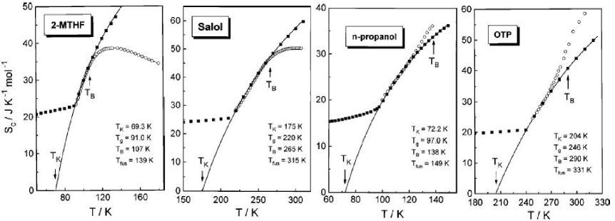
Figure 1.2: (From [6] and references therein) Configurational entropy $S_{c}(T)$ of four fragile glass formers. The black squares are obtained from calorimetric measurements of the specific heat of the liquid and of the crystal, see Eq. (1.4). Below $T_{g}$ (reported in the key) the liquid falls out of equilibrium. The black line is the extrapolation according to Eq. (1.5) of the equilibrium data for $T\geq T_{g}$ below $T_{g}$, that goes to zero at $T=T_{K}$. The open white circles are derived from the dielectric relaxation data of Fig. 1.1 using the Adam–Gibbs relation, Eq. (1.6). The coincidence of the two estimates of $S_{c}(T)$ proves the validity of the Adam–Gibbs relation for $T_{B}\geq T\geq T_{g}$.

The outcome of this procedure is that the configurational entropy seems to vanish at a finite temperature $T_{K}$. As $S_{c}$ counts the number of different structures that the liquid can access, it is not expected to become negative; also, negative values of $S_{c}$ imply that the entropy of the liquid becomes smaller than the entropy of the crystal, which is a very counterintuitive phenomenon. A possible explanation of this paradoxical behavior was proposed by Kauzmann [7], who argued that at some temperature between $T_{g}$ and $T_{K}$ the free energy barrier for crystal nucleation becomes of the order of the free energy barrier between different structures of the liquid. This means that the time scale for crystal nucleation becomes of the order of the structural relaxation time $\tau_{\alpha}$ of the liquid, and one cannot think anymore to an “equilibrium” liquid as crystallization will occur on the same time scale needed to equilibrate the liquid. The extrapolation of $S_{c}(T)$ down to $T_{K}$ is then meaningless, and the paradox is solved. This argument has been recently reconsidered, see e.g.  [8], and its implications are still under investigation.

1.1.4 The ideal glass transition

Alternatively, one can assume that the existence of the crystal is irrelevant, because crystallization can be in some way strongly inhibited: for instance, by considering binary mixtures, or –in numerical simulations– by adding a potential term to the Hamiltonian that forbids nucleation. If crystallization is neglected, the extrapolation of $S_{c}$ suggests that at $T_{K}$ a phase transition happens: at $T_{K}$, the number of structures available to the liquid is no more exponential, as $S_{c}=0$, and the system is frozen in one amorphous structure which can be called an ideal glass. Below $T_{K}$, the only contribution to the entropy of the ideal glass is the vibrational one, so the specific heat has a jump downward at $T_{K}$. The transition is expected to be of second order from a thermodynamical point of view.

An evidence that support this picture is the fact that in almost all the fragile glass formers it is found that $T_{K}\sim T_{0}$. For instance, in [2] some 30 cases where $T_{0}=T_{K}$ with an error of order $3\%$ are reported. This means that both the structural relaxation time and the viscosity diverge at $T_{K}$, so that the structures that are reached at $T_{K}$ are thermodynamically stable, being associated to an infinite structural relaxation time. The exact solution of a class of mean field disordered models which share many aspects of the phenomenology with fragile glass formers also supports the picture that a thermodynamic transition happens at $T_{K}$, as will be discussed later.

Of course, the ideal glass transition that occurs in equilibrium is not observable: at some temperature $T_{g}>T_{K}$ where $\tau_{\alpha}(T_{g})=\tau_{exp}$ a real glass transition, freezing the system in a nonequilibrium amorphous state (a real glass), happens. The value of $T_{g}$, as well as the properties of the nonequilibrium glass (density, structure, etc.) depend on the value of $\tau_{exp}$, which is usually $\sim 100$s as already discussed.

1.1.5 Adam–Gibbs relation

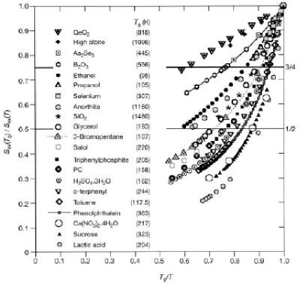
Figure 1.3: (From [3]) Scaled configurational entropy $S_{c}(T_{g})/S_{c}(T)$ (obtained from calorimetric data) for some of the substances of Fig. 1.2 as a function of $T_{g}/T$. The slope of the curves in $T=T_{g}$ is related to the fragility by Eq. (1.7).

The identity of $T_{0}$ and $T_{K}$ suggests that the divergence of $\tau_{\alpha}$ is related to the vanishing of $S_{c}$. Indeed, Adam and Gibbs [9] proposed that the following relation holds for $T$ close to $T_{g}$:

$$\tau_{\alpha}(T)=\tau_{\infty}\exp\left(\frac{{\cal E}}{TS_{c}(T)}\right)\ ,\hskip 20.0ptS_{c}(T)=\frac{{\cal E}}{T\log[\tau_{\alpha}(T)/\tau_{\infty}]}\ ,$$ (1.6)

where ${\cal E}$ is a system dependent parameter with the dimension of an energy that is somehow related to the energy barrier for activated processes of transition between different liquid structures. A similar relation for the viscosity is obtained by the Maxwell relation $\eta=G_{\infty}\tau_{\alpha}$. Eq. (1.6) has been successfully tested in a wide number of experiments and numerical simulations. As an example, in Fig. 1.2 the configurational entropy obtained from dielectric relaxation measurements of $\tau_{\alpha}$ via Eq. (1.6) is compared with the calorimetric measurement of $S_{c}$. The results show that Eq. (1.6) is very well satisfied in a range of temperatures above $T_{g}$.

The original Adam–Gibbs theory leading to Eq. (1.6) was reconsidered and improved in recent works [10, 11, 12, 13, 14], which will be discussed later.

Eq. (1.6) allows to rewrite the fragility defined by Angell as

$$\frac{m_{A}}{17}=1+\frac{T_{g}}{S_{c}(T_{g})}\frac{dS_{c}}{dT}(T_{g})=1+\left.\frac{d(S_{c}(T_{g})/S_{c}(T))}{d(T_{g}/T)}\right|_{T=T_{g}}\ .$$ (1.7)

As $T_{g}\frac{dS_{c}}{dT}(T_{g})$ is the specific heat jump at $T_{g}$, the Adam–Gibbs relation implies that fragility is linearly related to $\Delta C(T_{g})/S_{c}(T_{g})$. In Fig. 1.3 $S_{c}(T_{g})/S_{c}(T)$ is reported as a function of $T_{g}/T$ for many of the substances whose viscosity is reported in Fig. 1.1. The close similarity between the two plots is another indication of the validity of the Adam–Gibbs relation.

1.1.6 An order parameter for the glass transition

To better investigate the possibility that a thermodynamic transition happens at $T_{K}$, one should define an order parameter to discriminate between the liquid and the (ideal) glass phase [15]. Before going to a purely static description of the order parameter, it is easier to discuss a dynamical one. Around $T_{g}$, the dynamics of the particles happens on two time scales, the fast one related to the intra–cage motion, the slow one related to cooperative structural rearrangements. The latter are frozen at $T_{K}$: at an atomic level, one tends to associate the glass transition with the divergence of the time scale on which a given particle can get out of the cage made by its neighbors. While this is an intuitive picture, it is not possible to translate it into a good definition of an amorphous solid phase: because of the excitation and movements of vacancies and other defects, this individual trapping time scale is always finite, although it will increase exponentially when the temperature gets small. What is really divergent is the time scale needed for a large scale rearrangement of the structure. This means that, even if single particles can always escape their traps in finite time, in the thermodynamic limit density fluctuations remain partially correlated also for $t\rightarrow\infty$. Considering a system of $N$ particles, a proper dynamical definition of the order parameter is, for example, the so-called nonergodicity factor [15, 16]

$$f_{dyn}({\underline{k}})=\lim_{t\rightarrow\infty}\lim_{N\rightarrow\infty}\frac{1}{N}\sum_{jl}\langle e^{i{\underline{k}}\,[\,{\underline{x}}_{j}(t)-{\underline{x}}_{l}(0)\,]}\rangle=\lim_{t\rightarrow\infty}\lim_{N\rightarrow\infty}\langle\rho_{{\underline{k}}}(t)\rho_{-{\underline{k}}}(0)\rangle_{dyn}\ ,$$ (1.8)

where $x_{j}(t)$ is the position of particle $j$ at time $t$, ${\underline{k}}$ is an arbitrary wave vector of the order of magnitude of the inverse interparticle distance, $\rho_{{\underline{k}}}=N^{-1/2}\sum_{j}e^{i{\underline{k}}\,{\underline{x}}_{j}}$ is a Fourier component of the density fluctuations. The thermodynamic limit has to be taken first, because a finite number of particles always has a finite relaxation time. The average $\langle\bullet\rangle_{dyn}$ is on the dynamical history of a single system. $f_{dyn}({\underline{k}})$ is expected to vanish in the liquid phase and to be different from $0$ in the glass phase.

In order to construct a static order parameter, one needs to identify a macroscopic quantity that discriminates between the different equilibrium states that the system can access. Unfortunately, for amorphous states it is impossible to construct such a quantity: in the glass case, in order to choose a state, one should first know the average position of each particle in the solid, which requires an infinite amount of information. This situation is very different from the one that characterizes an ordered solid in which the Fourier components of the density $\rho_{{\underline{k}}}$ develop strong Bragg peaks in the solid phase. However, a simple method to deal with amorphous states has been developed in the context of spin glasses: the idea is to consider two identical copies of the original system coupled by a small extensive attraction of amplitude $\epsilon$. One takes first the thermodynamic limit, and then the limit $\epsilon\rightarrow 0$. In the liquid phase, the two copies are able to decorrelate also in the thermodynamic limit, while in the glass phase an infinitesimal attraction is enough to keep the copies close to each other. The order parameter is then defined as

$$f_{eq}({\underline{k}})=\lim_{\epsilon\rightarrow 0}\lim_{N\rightarrow\infty}\frac{1}{N}\sum_{jl}\langle e^{i{\underline{k}}\,[\,{\underline{x}}_{j}-{\underline{y}}_{l}\,]}\rangle_{\epsilon}\ ,$$ (1.9)

which is the static analogue of $f_{dyn}$. The average $\langle\bullet\rangle_{\epsilon}$ is now on the equilibrium distribution of the two coupled copies.

It is observed that $f({\underline{k}})$ jumps discontinuously to a finite value when crossing the glass transition temperature $T_{g}$. Thus, the glass transition is a second order transition from a thermodynamical point of view but it is of first order if one looks to the order parameter.

1.2 A mean field scenario

So far, the only systems for which the phenomenology described above could be analytically derived are some type of mean field spin glasses [10, 17, 18, 19, 20, 21, 22, 23, 24]: the so-called $p$-spin glasses. These systems show an equilibrium Kauzmann transition at a finite temperature $T_{K}$, where the configurational entropy vanishes, the specific heat jumps downward and the order parameter discontinuously jumps to a finite value. Their dynamics is very similar to the one of glass forming liquids in the region of temperature $T_{m}>T\gg T_{g}$, but the VFT behavior of the relaxation time is not reproduced by these models: instead, a power law divergence of the relaxation time is found at a temperature $T_{d}>T_{K}$. Although this phenomenon is due to the mean field nature of these models, it is not completely unrelated to what is observed in glass forming liquids, where a power law behavior of $\tau_{\alpha}$ is found at temperature $T$ not too close to $T_{g}$. Indeed, the equations that describe the dynamics of the $p$-spin glass models are formally very similar to the Mode–Coupling equations [25, 26] that describe well the dynamics of supercooled liquids in a range of temperature below $T_{m}$ but not too close to $T_{g}$ [28]. Moreover, many properties of the free energy landscape of these models (pure states, metastable states, barriers, etc.) could be investigated, allowing for a deep understanding of the mechanisms leading to the Kauzmann transition and to the slowing down of the dynamics close to $T_{d}$.

Excellent reviews on the properties of the $p$-spin models have been recently published [24, 27, 28]; in the following only the main results will be reviewed, referring to [24, 27, 28] and to the original papers [10, 17, 18, 19, 20, 21, 22, 23] for all the details.

1.2.1 Mean field $p$-spin models: the replica solution and the dynamics

The model is defined by the Hamiltonian

$$H_{p}(\sigma)=-\sum_{i_{1}<\cdots<i_{p}}J_{i_{1},\cdots,i_{p}}\sigma_{i_{1}}\cdots\sigma_{i_{p}}\ ,$$ (1.10)

where $\sigma_{i}$ are either real variables subject to a spherical constraint $\sum_{i}\sigma^{2}_{i}=N$, or Ising variables, $\sigma_{i}=\pm 1$, and $J_{i_{1},\cdots,i_{p}}$ are independent quenched random Gaussian variables with zero mean and variance $p!J^{2}/(2N^{p-1})$. The sum is over all the ordered $p$-uples of indices $i_{1}<\cdots<i_{p}$. It is a mean field model because each degree of freedom interact with all the others with a strength that vanishes in the thermodynamic limit, in order to have an extensive average energy.

The replica trick [29] allows to solve the model at all temperatures. A thermodynamic transition is found at $T_{K}$ corresponding to a $1$-step breaking of the replica symmetry (1rsb). At the transition, the specific heat jumps downward. The order parameter of the transition is the self-overlap between two different replicas $a$ and $b$:

$$q_{ab}\equiv\frac{1}{N}\sum_{i=1}^{N}\sigma_{i}^{a}\sigma_{i}^{b}\ ,$$ (1.11)

which plays the role, in the context of spin glass theory, of the nonergodicity factor (1.9). The average value of $q_{ab}$ jumps from $0$ to a finite value $q_{s}$ at $T_{K}$.

The Langevin dynamics of the model can also be solved exactly [28]. A dynamical transition is found at a temperature $T_{d}>T_{K}$; the relaxation time of the spin-spin autocorrelation function $C(t)=N^{-1}\sum_{i}\langle\sigma_{i}(t)\sigma_{i}(0)\rangle$ shows a power-law divergence for $T\rightarrow T_{d}$. A dynamical order parameter can be defined as

$$q_{d}=\lim_{t\rightarrow\infty}\lim_{N\rightarrow\infty}\frac{1}{N}\sum_{i}\langle\sigma_{i}(t)\sigma_{i}(0)\rangle=\lim_{t\rightarrow\infty}\lim_{N\rightarrow\infty}C(t)\ ;$$ (1.12)

it is the analogue of the dynamical nonergodicity factor defined in (1.8) and jumps to a finite value at $T_{d}$. Below $T_{d}$ the system is no more able to equilibrate with the thermal bath and enters a nonequilibrium regime. This result gives a strong indication that metastable states, which do not appear in the equilibrium calculation, are responsible for the slowing down of the dynamics and for the dynamical transition at $T_{d}$.

1.2.2 The TAP free energy

To better understand what is going on in the model one has to investigate the structure of its phase space. In particular, one wishes to characterize the equilibrium states in order to understand the nature of the thermodynamical transition at $T_{K}$, as well as the structure of the metastable states which seems to trap the system at $T_{d}$ and to be responsible for the existence of a dynamical transition. It turns out that a complete characterization of the structure of the states is possible by mean of the TAP free energy.

A general result of statistical mechachics (see e.g. [29, 30]) states that is always possible to decompose the equilibrium probability distribution as a sum over pure states:

$$P(\sigma_{1},\cdots,\sigma_{N})=\sum_{\alpha}w_{\alpha}P^{\alpha}(\sigma_{1},\cdots,\sigma_{N})\ ,$$ (1.13)

where $\alpha$ is an index labelling the states and $w_{\alpha}$ is the weight of each state, $\sum_{\alpha}w_{\alpha}=1$. The probability distributions of the pure states are characterized by the clustering property, that in mean field reads

$$P^{\alpha}(\sigma_{1},\cdots,\sigma_{N})=\prod_{i=1}^{N}P^{\alpha}_{i}(\sigma_{i})\ .$$ (1.14)

The single-spin probability distribution is in turn specified by the average magnetization of the spin $\sigma_{i}$, $m_{i}^{\alpha}=\sum_{\sigma}\sigma P^{\alpha}_{i}(\sigma)$. Thus, a pure state $\alpha$ is completely determined by the set of local magnetizations $m^{\alpha}_{i}$, $i=1,\cdots,N$. Moreover, a variational principle exists, stating that the local magnetizations of pure states must be minima of some free energy function $F(m_{i})$. This function, in the context of spin glasses, has the name of Thouless–Anderson–Palmer (TAP) free energy [29, 31].

The weight $w_{\alpha}$ of state $\alpha$ is proportional to $\exp[-\beta Nf_{\alpha}]$, where $f_{\alpha}=F(m_{i}^{\alpha})/N$. Thus, in the thermodynamic limit only the lowest free energy states are relevant. Local minima of $F$ having a free energy density $f>f_{min}$ for $N\rightarrow\infty$ are metastable states. The TAP free energy $F(m_{i})$ depend, in general, explicitly on the temperature, so the whole structure of the states may depend strongly on temperature.

Figure 1.4: (From [27]; $T_{s}$ corresponds to $T_{K}$, $T^{*}$ to $T_{d}$) Sketch of the evolution in temperature of the TAP states for the spherical $p$-spin model. Each TAP state like (4) can be followed in temperature until it becomes unstable and disappears. The complexity vanished continuously at the ground state $f_{min}$ (2) and goes abruptly to 0 above the maximum free energy $f_{max}$ (3). (5) is the free energy $f^{*}$ of the states that dominate the partition function. (1) is the equilibrium free energy $f^{*}-T\Sigma(f^{*})$ that takes into account the entropic contribution of the degeneracy of the states.

In mean field $p$-spin models, the expression of the TAP free energy can be explicitly derived [19, 20], and the distribution of the states can be computed. A peculiar property of the spherical $p$-spin model, which simplify a lot the description of the results of the TAP computation, is that the dependence of the free energy functional on $T$ is very simple. Indeed, the states are labeled by their energy $E$ at $T=0$. The number of states of energy $E$ is $\Omega(E)=\exp N\Sigma(E)$; the function $\Sigma(E)$ is called complexity: it is a concave function that vanishes continuously at the ground state energy $E_{min}$ and goes discontinuously to $0$ above some value $E_{max}$. At finite temperature, the minima get “dressed” by thermal fluctuations but they maintain their identity and one can follow their evolution at $T>0$. At some temperature $T_{max}(E)$, thermal fluctuations are so large that the states with energy $E$ become unstable and disappear, until, at high enough temperature $T>T_{TAP}$, only the paramagnetic minimum, $m_{i}\equiv 0$, survives.

At finite temperature, the number of states of given free energy density $f$ is $\Omega(f)=\exp N\Sigma(f)$, where $\Sigma(f)=\Sigma(E(f))$ and $E(f)$ is the $T=0$ energy of the states of free energy $f$. The function $\Sigma(f)$ vanishes continuously at $f=f_{min}$ and drops to zero above $f=f_{max}$; a qualitative plot of $\Sigma(f)$ is reported in Fig. 1.5. A similar behavior is found in all $p$-spins model like the Ising $p$-spin glass. The main peculiarity of $p$-spin models is that an exponential number of metastable states is present at low enough temperature.

One can write the partition function $Z$, at low enough temperature and for $N\rightarrow\infty$, in the following way:

$$\begin{split}Z=e^{-\beta NF(T)}\sim\sum_{\alpha}e^{-\beta Nf_{\alpha}}=\int_{f_{min}}^{f_{max}}df\,e^{N[\Sigma(f)-\beta f]}\sim e^{N[\Sigma(f^{*})-\beta f^{*}]}\ ,\end{split}$$ (1.15)

where $f^{*}\in[f_{min},f_{max}]$ is such that $\Phi(f)=f-T\Sigma(f)$ is minimum, i.e. it is the solution of

$$\frac{d\Sigma}{df}=\frac{1}{T}\ ,$$ (1.16)

provided that it belongs to the interval $[f_{min},f_{max}]$. Starting from high temperature, one encounters three temperature regions:

• For $T>T_{d}$, the free energy density of the paramagnetic state is smaller than $f-T\Sigma(f)$ for any $f\in[f_{min},f_{max}]$, so the paramagnetic state dominates and coincides with the Gibbs state (in this region the decomposition (1.15) is meaningless).

• For $T_{d}\geq T\geq T_{K}$, a value $f^{*}\in[f_{min},f_{max}]$ is found, such that $f^{*}-T\Sigma(f^{*})$ is equal to $f_{para}$. This means that the paramagnetic state is obtained from the superposition of an exponential number of pure states of higher individual free energy density $f^{*}$. The Gibbs measure is splitted on this exponential number of contributions: however, no phase transition happens at $T_{d}$ because of the equality $f^{*}-T\Sigma(f^{*})=f_{para}$ which guarantees that the free energy is analytic on crossing $T_{d}$.

• For $T<T_{K}$, the partition function is dominated by the lowest free energy states, $f^{*}=f_{min}$, with $\Sigma(f_{min})=0$ and $F(T)=f_{min}-T\Sigma(f_{min})=f_{min}$. At $T_{K}$ a phase transition occurs, corresponding to the 1-step replica symmetry breaking transition found in the replica computation.

In the range of temperatures $T_{d}>T>T_{K}$, the phase space of the model is disconnected in an exponentially large number of states, giving a contribution $\Sigma(T)\equiv\Sigma(f^{*}(T))$ to the total entropy of the system. This means that the entropy $S(T)$ for $T_{d}>T>T_{K}$ can be written as

$$S(T)=\Sigma(T)+S_{vib}(T)\ ,$$ (1.17)

$S_{vib}(T)$ being the individual entropy of a state of free energy $f^{*}$. From the latter relation it turns out that the complexity $\Sigma(T)$ is the $p$-spin analogue of the configurational entropy $S_{c}(T)$ of supercooled liquids.

The TAP approach provides also a pictorial explaination of the presence of a dynamical transition at $T_{d}$. If the system is equilibrated at high temperature in the paramagnetic phase, and suddenly quenched below $T_{d}$, the energy density start to decrease toward its equilibrium value. This relaxation process can be represented as a descent in the free energy landscape at fixed temperature starting from high values of $f$. What happens is that when the sistem reaches the value $f_{max}$ it becomes trapped in the highest metastable state and is unable to relax to the equilibrium states of free energy $f^{*}$, as the free energy barriers between different states cannot be crossed in mean field [27, 28]. For this reason below $T_{d}$ the systems is unable to equilibrate. What happens in real glasses is that activated processes of jump between different metastable states allow the system to relax toward equilibrium also below $T_{d}$. Activated processes give rise to the VFT behavior of the relaxation time, as will be discussed in the following.

1.3 Two methods to compute the complexity

If a given system presents a structure of the free energy landscape similar to $p$-spin glasses, two general methods to compute the complexity as a function of the free energy of the states without directly solving the TAP equations exist; they have been developed in [15, 35, 36, 37, 38, 39, 40, 41]. Both methods consider a number of copies of the system coupled by a small field conjugated to the order parameter (1.9).

1.3.1 Real replica method

Figure 1.5: (From [15]) A sketch of the complexity as a function of the free energy density for system belonging to the $p$-spin class. The value $f^{*}(m,T)$, solution of $\frac{d\Sigma}{df}=\frac{m}{T}$, is also reported.

The idea of [15, 37] is to consider $m$ copies of the original system, coupled by a small attractive term added to the Hamiltonian. The coupling is then switched off after the thermodynamic limit has been taken. For $T<T_{d}$, the small attractive coupling is enough to constrain the $m$ copies to be in the same TAP state. At low temperatures, the partition function of the replicated system is then

$$Z_{m}=e^{-\beta N\Phi(m,T)}\sim\sum_{\alpha}e^{-\beta Nmf_{\alpha}}=\int_{f_{min}}^{f_{max}}df\,e^{N[\Sigma(f)-\beta mf]}\sim e^{N[\Sigma(f^{*})-\beta mf^{*}]}\ ,$$ (1.18)

where now $f^{*}(m,T)$ is such that $\Phi(m,f)=mf-T\Sigma(f)$ is minimum and satisfies the equation

$$\frac{d\Sigma}{df}=\frac{m}{T}\ .$$ (1.19)

If $m$ is allowed to assume real values by an analytical continuation, the complexity can be computed from the knowledge of the function $\Phi(m,T)=mf^{*}(m,T)-T\Sigma(f^{*}(m,T))$. Indeed, it is easy to show that

$$\begin{split}&f^{*}(m,T)=\frac{\partial\,\Phi(m,T)}{\partial m}\ ,\\ &\Sigma(m,T)=\Sigma(f^{*}(m,T))=m^{2}\frac{\partial\,[m^{-1}\beta\Phi(m,T)]}{\partial m}=m\beta f^{*}(m,T)-\beta\Phi(m,T)\ .\end{split}$$ (1.20)

The function $\Sigma(f)$ can be reconstructed from the parametric plot of $f^{*}(m,T)$ and $\Sigma(m,T)$ by varying $m$ at fixed temperature.

The glass transition happens when $\beta$ equals the slope $s_{0}(T)$ of $\Sigma(f)$ in $f=f_{min}$, so $T_{K}$ is defined by $T_{K}s_{0}(T_{K})=1$. If $m<1$, the value of $f^{*}(m,T)$ correspond to a smaller slope with respect to $m=1$, so the glass transition is shifted towards lower values of the temperature, see Fig. 1.5. For any value of the temperature $T$ below $T_{K}$ it exists a value $m^{*}(T)<1$ such that for $m<m^{*}$ the system is in the liquid phase. The free energy for $T<T_{K}$ and $m<m^{*}(T)$ can be computed by analytic continuation of the free energy of the high temperature liquid. As the free energy is always continuous and it is independent of $m$ in the glass phase (being simply the value $f_{min}(T)$ such that $\Sigma(f_{min})=0$), one can compute the free energy of the glass below $T_{K}$ simply as $F_{glass}(T)=f_{min}(T)=\Phi(m^{*}(T),T)/m^{*}(T)$.

This method allows to compute the complexity as well as the free energy of the glass, i.e. of the lowest free energy states, at any temperature, if one is able to compute the free energy of $m$ copies of the original system constrained to be in the same free energy state and to perform the analytical continuation to real $m$. In [40] it was applied to the spherical $p$-spin system and it was shown that the method reproduces the results obtained from the explicit TAP computation.

1.3.2 Potential method

The second method [35, 36, 38, 39] starts from a reference configuration $\sigma$ of the original system and consider the partition function of an identical system $\tau$ which Hamiltonian has been corrected by the addition of a coupling to the configuration $\sigma$:

$$Z(\sigma,\epsilon,T)=\int d\tau\,e^{-\beta H(\tau)+\beta N\epsilon q(\sigma,\tau)}\ ,$$ (1.21)

where $q(\sigma,\tau)=N^{-1}\sum_{i}\sigma_{i}\tau_{i}$ as in (1.11). If the reference configuration $\sigma$ is extracted from the equilibrium distribution at temperature $T$, the free energy $F(\sigma,\epsilon,T)=-TN^{-1}\log Z(\sigma,\epsilon,T)$ should not depend on the particular choice of $\sigma$ for $N\rightarrow\infty$. Thus one averages over the equilibrium distribution of $\sigma$ at temperature $T$ and defines

$$F(\epsilon,T)=-\frac{T}{N}\int d\sigma\frac{e^{-\beta H(\sigma)}}{Z(\beta)}\log Z(\sigma,\epsilon,T)\ .$$ (1.22)

If, in the limit $\epsilon\rightarrow 0$, the correlation between $\sigma$ and $\tau$ is lost, one has $F(\epsilon=0,T)=F(T)$. Otherwise, one can study the effect of the correlation in the limit of vanishing coupling between the replicas.

Being interested in the behavior at $\epsilon=0$, one considers the Legendre transform of $F(\epsilon,T)$,

$$V(q,T)=\max_{\epsilon}\big{[}F(\epsilon,T)+\epsilon q\big{]}\ ,\hskip 20.0ptq(\epsilon)=-\frac{\partial F(\epsilon,T)}{\partial\epsilon}=\langle q(\sigma,\tau)\rangle_{\epsilon}\ .$$ (1.23)

The thermodynamic potential $V(q,T)$ is the free-energy of the system $\tau$ constrained to be at a fixed overlap $q$ with $\sigma$:

$$\begin{split}&V(q,T)=-\frac{T}{N}\int d\sigma\frac{e^{-\beta H(\sigma)}}{Z(\beta)}\log Z(\sigma,q,T)\ ,\\ &Z(\sigma,q,T)=\int d\tau\,e^{-\beta H(\tau)}\delta(q-q(\sigma,\tau))\ .\end{split}$$ (1.24)

As $\frac{dV}{dq}=\epsilon(q)$, the average value of the order parameter in the limit $\epsilon\rightarrow 0$ is the value of $q$ that solves $\frac{dV}{dq}=0$; the minima of $V(q)$ correspond to the possible phases in the limit of zero coupling.

The qualitative behavior of $V(q,T)-F(T)$ is shown in Fig. 1.6 for the spherical mean field $p$-spin model: for $T>T_{d}$ it is a convex function of $q$ with only one minimum at $q=0$. At the dynamical transition temperature $T_{d}$ a secondary minimum starts to develop at finite $q$. On lowering the temperature below $T_{d}$, the value of $V$ at the minimum decreases and vanishes at the thermodynamical transition temperature $T_{K}$. Indeed, for $T>T_{d}$ there is only one phase in which the two copies $\sigma$ and $\tau$ are uncorrelated and the average overlap vanishes. Below $T_{d}$, a new phase in which the two copies are in the same TAP state appears; this phase is metastable because there is an exponential number of TAP states so the probability of finding the two copies in the same state is exponentially small in absence of coupling. The value of $q$, $q_{min}(T)$, corresponding to this secondary minimum is the self-overlap of the equilibrium TAP states at temperature $T$. For $T<T_{K}$, the value of $V(q_{min})$ becomes equal to $V(0)$, as the number of states is no more exponential and a vanishing coupling is enough to constrain the two copies to be in the same state. This correspond to the 1rsb phase transition. This approach underlines the first order nature of the transition from the point of view of the order parameter.

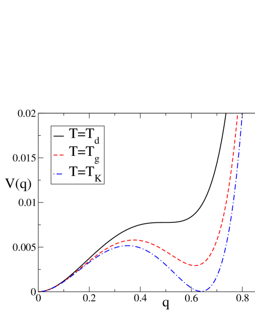
Figure 1.6: The two-replica potential, $V(q,T)-F(T)$, for $T$$\in$$[T_{K},T_{d}]$ in the spherical $p$-spin model.

The value of $V(q,T)$ at the secondary minimum for $T$$\in$$[T_{K},T_{d}]$, i.e. the average free energy of the configuration $\tau$ at $q=q_{min}=q(T)$, is the free energy $f^{*}(T)$ of the equilibrium TAP states. From Eq. (1.24), recalling that $F(T)=f^{*}(T)-T\Sigma(f^{*}(T))$, one has

$$V(q_{min}(T),T)-V(0,T)=f^{*}(T)-F(T)=T\Sigma(f^{*}(T))\ ,$$ (1.25)

where $\Sigma(f^{*}(T))$ is the equilibrium complexity. The vanishing of $V(q_{min}(T_{K}),T_{K})-F(T_{K})$ corresponds to the vanishing of the complexity at $T_{K}$.

From the potential $V(q,T)$ one can extract the values of the dynamical and thermodynamical transitions as well as the free energy of the equilibrium states $f^{*}(T)$ and their complexity $\Sigma(f^{*}(T))$. To obtain informations about the metastable TAP states one needs to consider a reference configuration equilibrated at a different temperature $T^{\prime}$:

$$\begin{split}&V(q,T,T^{\prime})=-\frac{T}{N}\int d\sigma\frac{e^{-\beta^{\prime}H(\sigma)}}{Z(\beta^{\prime})}\log Z(\sigma,q,T)\ ,\\ &Z(\sigma,q,T)=\int d\tau\,e^{-\beta H(\tau)}\delta(q-q(\sigma,\tau))\ .\end{split}$$ (1.26)

If $T^{\prime}$$\in$$[T_{K},T_{d}]$ and if the evolution of the TAP states in temperature is described by the curves in Fig. 1.4, the configuration $\sigma$ is in one of the equilibrium TAP states at temperature $T^{\prime}$, while the configuration $\tau$ is constrained to be close to it (i.e. in the same TAP state) but at temperature $T$. The free energy of $\tau$ for $q=q_{min}(T,T^{\prime})$ is the free energy of an equilibrium TAP state at temperature $T^{\prime}$ when followed at temperature $T$. The TAP states are labeled by their zero-temperature energy $E$; their free energy is $f_{TAP}(E,T)$. Thus one has

$$V(q_{min}(T,T^{\prime}),T,T^{\prime})=f_{TAP}(E(T^{\prime}),T)\ ,$$ (1.27)

where $E(T^{\prime})$ is the $T=0$ energy of the equilibrium TAP states at temperature $T^{\prime}$ and $f^{*}(T^{\prime})=f_{TAP}(E(T^{\prime}),T^{\prime})$.

The procedure to compute the properties of all the TAP states using the potential method is the following:

• First one consider the potential for $T=T^{\prime}$ and computes the free energy $f^{*}(T)$ and the complexity $\Sigma(f^{*}(T))$ for $T$$\in$$[T_{K},T_{d}]$. This give access to the complexity $\Sigma(f)$.

• Then one fixes $T^{\prime}$$\in$$[T_{K},T_{d}]$ and computes, using Eq. (1.27) the free energy $f_{TAP}(E(T^{\prime}),T)$ as a function of $T$ down to $T=0$.

• In particular, the free energy of the glass (i.e. of the lowest TAP states) is obtained considering the limit $T^{\prime}\rightarrow T_{K}$ (from above) in Eq. (1.27).

It was shown in [36, 38] that the result is consistent with the direct computation using the TAP equations.

1.3.3 Connection with the standard replica method

It is interesting to consider the relation between the two methods described above and the 1rsb free energy, also because some of the formulae will be useful in the applications of the next chapters.

In the spherical $p$-spin model, the average over the distribution of the couplings $J$ (indicated by an overbar) of the $n$ times replicated partition function can be rewritten as [21]

$$\begin{split}&\overline{Z^{n}(J)}=\overline{\left(\int d\sigma e^{-\beta H(\sigma)}\right)^{n}}=\overline{\int d\sigma_{a}e^{-\beta\sum_{a}H(\sigma_{a})}}=\int dQ_{ab}\ e^{Nf(Q)}\ ,\\ &f(Q)=\frac{\beta^{2}}{4}\sum_{ab}Q_{ab}^{p}+\frac{1}{2}\log\det Q\ ,\end{split}$$ (1.28)

where $a,b=1,\cdots,n$ and $Q_{ab}$ in the $n\times n$ overlap matrix [29]. The substitution of the 1rsb ansatz for $Q$ (in the example, $n=6$ and $m=3$):

$${\cal Q}=\left(\begin{array}[]{cc}\left(\begin{array}[]{ccc}1&q&q\\ q&1&q\\ q&q&1\\ \end{array}\right)&0\\ 0&\left(\begin{array}[]{ccc}1&q&q\\ q&1&q\\ q&q&1\\ \end{array}\right)\\ \end{array}\right)$$

in Eq. (1.28) gives, for $N\rightarrow\infty$,

$$\begin{split}&\overline{Z^{n}}\sim\exp\big{[}-\beta nN\phi_{1RSB}(m^{*},q^{*},T)\big{]}\ ,\\ &F(T)=-\frac{T}{N}\lim_{n\rightarrow 0}\partial_{n}\overline{Z^{n}}=\phi_{1RSB}(m^{*},q^{*},T)\ ,\end{split}$$ (1.29)

where the 1rsb free energy is

$$\phi_{1RSB}(m,q,T)=-\frac{1}{2\beta}\left\{\frac{\beta^{2}}{2}\big{[}1+(m-1)q^{p}\big{]}+\frac{m-1}{m}\log(1-q)+\frac{1}{m}\log\big{[}1+(m-1)q\big{]}\right\}\ ,$$ (1.30)

and $m^{*}$, $q^{*}$ are solutions of $\partial_{m}\phi_{1RSB}=0$ and $\partial_{q}\phi_{1RSB}=0$. For $T>T_{K}$ the solution $q^{*}=0$, $m^{*}=1$ is the stable one, even if a solution with $q^{*}\neq 0$ appears for $T<T_{d}$. Below $T_{K}$ this solution, with $q^{*}\neq 0$ and $m^{*}<1$, is the free energy of the glass.

Real replica method

In the real replica method the partition function of $m$ copies of the system is considered. Using the replica trick to compute the free energy,

$$\Phi(m,T)=-\frac{T}{N}\overline{\log Z_{m}}=-\frac{T}{N}\lim_{n\rightarrow 0}\partial_{n}\overline{(Z_{m})^{n}}=-\frac{T}{N}\lim_{n\rightarrow 0}\partial_{n}\overline{Z^{mn}}\ ,$$ (1.31)

one obtains the partition function of $nm$ copies of the system, with the constraint that each block of $m$ replicas has to be in the same state. This leads naturally to the 1rsb structure for the overlap matrix (with $m$ fixed) and

$$\Phi(m,T)=-\frac{T}{N}\lim_{n\rightarrow 0}\partial_{n}\exp\big{[}-\beta nmN\phi_{1RSB}(m,q^{*},T)\big{]}=m\phi_{1RSB}(m,q^{*},T)\ .$$ (1.32)

Note that the hypothesis that the $m$ replicas are in the same state implies that for any value of $(m,T)$ the correct solution is the one with $q^{*}\neq 0$. Above $T_{d}$ this solution disappears as a vanishing coupling cannot constrain the replicas to stay close to each other.

The free energy of the real replica method is the 1rsb free energy as a function of $m$ at the value $q^{*}\neq 0$ that solves $\partial_{q}\phi_{1RSB}=0$. Using Eq. (1.20) the complexity as a function of $m$ is

$$T\Sigma(m,T)=m^{2}\partial_{m}\big{[}m^{-1}\Phi(m,T)\big{]}=m^{2}\partial_{m}\phi_{1RSB}(m,q^{*},T)\ ,$$ (1.33)

and the equilibrium complexity is

$$\Sigma(T)=\Sigma(1,T)=-\frac{1}{2}\left[\frac{\beta^{2}}{2}(q^{*})^{p}+\log(1-q^{*})+q^{*}\right]\ .$$ (1.34)

As $\Sigma(m,T)\propto\partial_{m}\phi_{1RSB}$, the value $m^{*}$ that optimizes the 1rsb free energy below $T_{K}$ coincides with the value $m^{*}$ defined by $\Sigma(m^{*},T)=0$ of the real replica method.

Potential method

Using the replica trick [36] the following expression for $V(q,T,T^{\prime})$ is derived:

$$V(q,T,T^{\prime})=-\lim_{n\rightarrow 0}\lim_{m\rightarrow 1}\frac{T}{Nn}\frac{\partial}{\partial m}\overline{\left(\int d\sigma\,e^{-\beta^{\prime}H(\sigma)}Z(\sigma,q,T)^{m-1}\right)^{n}}\ .$$ (1.35)

The last integral can be rewritten as

$$\left(\int d\sigma\,e^{-\beta^{\prime}H(\sigma)}Z(\sigma,q,T)^{m-1}\right)^{n}=\int d\sigma_{a\alpha}e^{-\sum_{a\alpha}\beta_{\alpha}H(\sigma_{a\alpha})}\prod_{a=1}^{n}\prod_{\alpha=2}^{m}\delta(q-q(\sigma_{a1},\sigma_{a\alpha}))\ ,$$ (1.36)

where $a=1,\cdots,n$, $\alpha=1,\cdots,m$, and $\beta_{\alpha}=\beta^{\prime}\delta_{1\alpha}+\beta(1-\delta_{1\alpha})$. This is again the expression of the $nm$ times replicated equilibrium partition function, with the additional constraint given by the $\delta$-functions. The average over the disorder gives

$$\begin{split}&\int dQ_{a\alpha,b\beta}\ e^{Nf(Q)}\ \prod_{a=1}^{n}\prod_{\alpha=2}^{m}\delta(q-Q_{a1,a\alpha})\ ,\\ &f(Q)=\frac{1}{4}\sum_{a\alpha,b\beta}\beta_{\alpha}\beta_{\beta}Q_{a\alpha,b\beta}^{p}+\frac{1}{2}\log\det Q\ .\end{split}$$ (1.37)

Evaluating the integral at the saddle point, one has

$$V(q,T,T^{\prime})=-\lim_{n\rightarrow 0}\lim_{m\rightarrow 1}\frac{T}{n}\frac{\partial}{\partial m}f(\overline{Q})\ .$$ (1.38)

The matrix $\overline{Q}$ is defined by the following conditions:
i) the elements on the diagonal are equal to 1;
ii) the elements $\overline{Q}_{a1a\alpha}$, $\alpha>1$, are equal to $q$;
iii) all the other elements are determined by the maximization of $f(Q)$.
As usual, one needs a parametrization of the matrix $Q$ in order to perform the analytic continuation to non-integer $n$ and $m$. A possible ansatz is [36] (in the example, $n=2$, $m=4$):

$$\overline{Q}=\left(\begin{array}[]{cc}\left(\begin{array}[]{cccc}1&q&q&q\\ q&1&r&r\\ q&r&1&r\\ q&r&r&1\\ \end{array}\right)&0\\ 0&\left(\begin{array}[]{cccc}1&q&q&q\\ q&1&r&r\\ q&r&1&r\\ q&r&r&1\\ \end{array}\right)\\ \end{array}\right)\ .$$ (1.39)

and corresponds to the following structure: each replica of $\sigma$ is independent from the others, and for each $\sigma$ there are $m-1$ copies of $\tau$ which have overlap $q$ with $\sigma$ and overlap $r$ within themselves. Within this ansatz, and using the relation

$$\det\left(\begin{array}[]{cccc}1&q&q&q\\ q&1&r&r\\ q&r&1&r\\ q&r&r&1\\ \end{array}\right)=(1-r)^{m-2}[1-2r+rm-(m-1)q^{2}]\ ,$$ (1.40)

one gets

$$V(q,T,T^{\prime})=-\frac{1}{2\beta}\left[\beta\beta^{\prime}q^{p}-\frac{\beta^{2}r^{p}}{2}+\frac{\beta^{2}}{2}+\log(1-r)+\frac{r-q^{2}}{1-r}\right]\ ,$$ (1.41)

where $r(q)$ is determined by $\partial_{r}V=0$.

For $T=T^{\prime}\geq T_{K}$ it is easy to check that the condition $\frac{dV}{dq}=\partial_{q}V=0$, together with $\partial_{r}V=0$, is satisfied if $q=r$. Thus, when $V(q)$ is stationary, $r(q)=q$ and the potential $V(q)$ reduces to

$$V(q,T)=-\frac{\beta}{4}-\frac{\beta q^{p}}{4}-\frac{T}{2}\big{[}\log(1-q)+q\big{]}=F(T)+\lim_{m\rightarrow 1}\partial_{m}\phi_{1RSB}(m,q,T)\ .$$ (1.42)

The latter relation can be proven in general and follows from the observation that when $\frac{dV}{dq}=0$ the matrix ${\overline{Q}}$ reduces to the usual 1rsb overlap matrix ${\cal Q}$. This is because the condition $\frac{dV}{dq}=\partial_{q}V=0$ together with $\partial_{r}V=0$ is equivalent, from Eq. (1.38), to

$$\frac{df(Q)}{dQ}=0\ .$$ (1.43)

This means that the function $f(Q)$ must be stationary with respect to all the elements of $Q$, and the 1rsb matrix ${\cal Q}$ provides a solution to this condition. If ${\overline{Q}}={\cal Q}$, one has

$$\frac{f({\overline{Q}})}{nm}=-\beta\phi_{1RSB}(m,q,T)\ .$$ (1.44)

Substituting this expression in Eq. (1.38), one obtains

$$V(q,T)=\lim_{m\rightarrow 1}\partial_{m}\Big{(}m\phi_{1RSB}(m,q,T)\Big{)}=F(T)+\lim_{m\rightarrow 1}\partial_{m}\phi_{1RSB}(m,q,T)\ ;$$ (1.45)

using the relation $\phi_{1RSB}(m=1)=F(T)$ that holds above $T_{K}$. Therefore, on its stationary points, $V(q,T)$ is given (at the 1rsb level) by this simple expression, that can be easily calculated in several models. Note that, as discussed in [39], full RSB effects can be important for the computation of $V(q,T)$ even in 1rsb models such as the $p$-spin spherical model.

If $T^{\prime}=T_{K}$ and $T<T_{K}$, the value of $V$ in the secondary minimum can still be computed using the simple ansatz (1.39). It can be seen, using the relation

$$\frac{T}{T_{K}}=m^{*}\left[\frac{1+(m^{*}-1)q^{*}}{m^{*}}\right]^{p/2}\ ,$$ (1.46)

that follows from the equations that define $m^{*}$ and $q^{*}$, that the solutions to $\partial_{r}V=0$, $\partial_{q}V=0$, is

$$\begin{cases}&r=q^{*}\ ,\\ &q=q^{*}\sqrt{\frac{m^{*}}{1+(m^{*}-1)q^{*}}}\ .\\ \end{cases}$$ (1.47)

Indeed $r$ is the self–overlap of the replicas inside the equilibrium states at $T_{K}$, so it is equal to the self–overlap $q^{*}$ of the glass. Substituting these espressions in $V(q,T,T^{\prime})$ one obtains

$$V(q_{min},T,T_{K})=\phi_{1RSB}(m^{*},q^{*},T)=F_{glass}(T)\ ,$$ (1.48)

as expected from Eq. (1.27).

Discussion

The explicit relation between the free energies $\Phi(m,T)$ and $V(q,T,T^{\prime})$ and the 1rsb free energy $\phi_{1RSB}(m,q,T)$ derived for the spherical $p$-spin model confirms that:

• the real replica potential $\Phi(m,T)$ is related to the 1rsb free energy as a function of $m$ for $q=q^{*}(m,T)\neq 0$. For this reason it allows to study the properties in the glass phase at $m=m^{*}<1$. Remarkably, it also allows to compute the free energy of the metastable states and their complexity for $T$$\in$$[T_{K},T_{d}]$.

• the potential $V(q,T,T^{\prime})$ for $T=T^{\prime}$ is related to the (derivative of the) 1rsb free energy at $m=1$, as a function of $q$. Thus it is not suitable to study the region below $T_{K}$ where $m\neq 1$, but it allows to study in detail the properties of the intermediate phase $T$$\in$$[T_{K},T_{d}]$, in particular the metastability of the $q\neq 0$ phase for $T$$\in$$[T_{K},T_{d}]$ and to estimate the barrier between the metastable and stable regions [44, 46].

• to compute the free energy of the metastable states and, as a particular case, the free energy of the glass, one needs to consider an extended definition of the potential, $V(q,T,T^{\prime})$, see Eq. (1.26). The relation between this potential and $\phi_{1RSB}$ is more involved, but at least for $T^{\prime}=T_{K}$ one has $V(q_{min},T,T_{K})=\phi_{1RSB}(m^{*},q^{*},T)=F_{glass}(T)$.

1.4 Beyond mean field

The random first order scenario that emerges from the analytical solution of $p$-spin disordered models explains most of the phenomenology of the glass transition. However, some big issues remain unexplained. The main problem of the mean field approach –as usual– is the existence of metastable states with intensive free energy higher than the free energy of the ground states, $f>f_{min}$. These states are responsible for the existence of a finite complexity. Their lifetime is infinite, so they are able to trap the system below $T_{d}$. This is the reason why the dynamical transition, i.e. the divergence of the structural relaxation time, happens at a temperature $T_{d}>T_{K}$.

In a model with short range interactions, metastable states have a finite lifetime due to the nucleation of bubbles of the stable phase inside the metastable one, so they are not thermodynamically stable. One should expect the existence of well defined states with $f>f_{min}$ to be impossible; but the analogy between mean field models and real glasses is mainly based on the analogy between the complexity $\Sigma(T)$ and the configurational entropy $S_{c}(T)$. How can one explain the existence of a finite configurational entropy, related to well defined metastable states, in a short range system?

Moreover, the observed crossover of the relaxation time from a power–law behavior to a Vogel–Fulcher–Tamman law (1.1) as well as the Adam–Gibbs relation (1.6) are not explained by the mean field theory, which predicts a strict power–law divergence of $\tau_{\alpha}$ for $T\rightarrow T_{d}^{+}$. The observation of a finite relaxation time below $T_{d}$ is again related to the finite lifetime of metastable states. The system, instead of being trapped forever into a state, is able to escape, due to nucleation processes; it is then trapped by another state, and so on. These processes of jump between metastable states are activated processes: the system has to cross some free energy barrier in order to jump from one state to another. The relaxation time is then expected to scale as

$$\tau_{\alpha}(T)\sim\tau_{\infty}\exp\big{[}\beta\Delta F(T)\big{]}\ ,$$ (1.49)

$\Delta F(T)$ being the typical free energy barrier that the system has to cross at temperature $T$. The VFT law and the observation that $T_{0}\sim T_{K}$ suggest that the barrier should diverge at $T_{K}$, $\Delta F(T)\sim(T-T_{K})^{-1}$; more generally, the Adam–Gibbs formula relates this divergence to the vanishing of the configurational entropy, $\Delta F(T)\sim S_{c}(T)^{-1}$. It is then essential to understand what is really the meaning of $S_{c}(T)$ in finite dimension and why it is related to the free energy barrier for nucleation.

A crucial observation is that the divergence of the relaxation time at $T_{K}$, in short range systems, is possible only if the cooperative processes of structural rearrangement involve atoms that are correlated on a typical length scale $\xi$, which diverges at $T_{K}$. If no divergent length scale is present in the system, it is always possible to divide it in finite subsystems, each one relaxing independently of the others: and the relaxation of a finite system usually happens in finite time, if the interactions are finite and have short range.

A simple idea that follows from the above observation and can explain how the mean field picture is modified in short range systems is the following [10, 11, 12, 13, 14, 42, 43, 45, 46, 47]. It exists a typical lenght scale $\xi(T)$ over which structural relaxation processes happens. If one looks at smaller length scales, the system behaves as if it were mean field: metastable states are stable for $l<\xi$, yielding a finite local complexity. However, for large scales $l>\xi$, metastability is destroyed and only the lowest free energy states are stable. For $T\rightarrow T_{K}^{+}$, $\xi\rightarrow\infty$, so below $T_{K}$ a stable ideal glass phase is possible. This idea leads naturally to the identification of the configurational entropy $S_{c}(T)$ with the local complexity $\Sigma(T)$, and to a derivation of an Adam-Gibbs–like relation between the relaxation time $\tau_{\alpha}$ and $\Sigma(T)$.

1.4.1 Dynamical heterogeneities: a derivation of the Adam-Gibbs relation

The above considerations can be formalized as follows [14]. An homogeneous equilibrium state in a finite dimensional system is defined as the probability distribution that is reached in each finite volume inside the container when the thermodynamic limit is taken with a given sequence of boundary conditions [30]: e.g. for a ferromagnet at low temperatures the two states $+$ and $-$ can be obtained taking the thermodynamic limit with the spins on the boundary fixed to $+$ or $-$, respectively.

For glassy systems this simple procedure does not work because the order parameter (1.8) is the self–overlap of the configurations of the same system for $t\rightarrow\infty$ or, equivalently, the overlap (1.9) between two coupled copies of the system, and it is not clear how to fix it using boundary conditions.

To overcome this problem, assume that an equilibrium state $\alpha$ of free energy density $f_{\alpha}$ exists. Assume also that a whole distribution of states of complexity $\Sigma(f)$ (per unit volume) exists for $f\in[f_{min},f_{max}]$. Then, consider a configuration belonging to the state $\alpha$ and a bubble of radius $R$ inside the system; all the particles outside the bubble are frozen in their position and act as boundary terms, and one consider the partition function of the bubble in presence of these boundary conditions. The idea is to find a self–consistency condition for the radius of the bubble $R$ requesting that the particles inside the bubble remain in the state $\alpha$ due to the boundary conditions.

The partition function of the bubble is

$$Z_{R}\sim e^{-\beta f_{\alpha}R^{d}}+\sum_{\gamma\neq\alpha}e^{-\beta f_{\gamma}R^{d}-\beta\Upsilon R^{\theta}}=e^{-\beta f_{\alpha}R^{d}}+\int_{f_{min}}^{f_{max}}df\,e^{\Sigma(f)R^{d}-\beta fR^{d}-\beta\Upsilon R^{\theta}}\ .$$ (1.50)

The first term represents the bubble in the same state $\alpha$ of the particles outside the boundary, while the second term represents the situation where the bubble is in a different state. In this case, the term $\beta\Upsilon R^{\theta}$ represents the free energy cost of the interface between the states $\alpha$ and $\gamma$ at the boundary of the bubble, which should scale as $R^{\theta}$ with $\theta\leq d-1$ if the interactions have short range. If the state $\alpha$ is chosen to be an equilibrium state, of energy $f_{\alpha}=f^{*}$ such that $\frac{d\Sigma}{df}(f^{*})=\beta$, the partition function becomes

$$Z_{R}\sim e^{-\beta f^{*}R^{d}}+e^{\Sigma(f^{*})R^{d}-\beta f^{*}R^{d}-\beta\Upsilon R^{\theta}}\ ,$$ (1.51)

where $\Sigma(f^{*}(T))=\Sigma(T)$ is the equilibrium complexity as usual. It is clear that if $\Sigma(f^{*})R^{d}-\beta\Upsilon R^{\theta}>0$, the second term dominates and the bubble is in a different state, otherwise the first term dominates and the boundary conditions are able to keep the particles inside the bubble in the state $\alpha$. If the bubble is in the state $\alpha$ it gains the term due to the interface, $\beta\Upsilon R^{\theta}$; however the probability of changing state is very large due to the exponential degeneracy of the states, as expressed by the term $\Sigma(T)R^{d}$. In this sense, one can think to $\Delta F_{v}(T)=-T\Sigma(T)$ as the bulk free energy gain that drives the escape from the state $\alpha$: it is not a free energy difference between the stable and metastable phase, as in ordinary nucleation problems, rather it is the contribution coming from the large number of possibilities that one has to choose a different state with the same free energy density.

As $\theta\leq d-1$ in short range systems, it is clear that for $R\rightarrow\infty$ the second term is always dominant and the bubble always escapes from the state $\alpha$. This implies that the initial assumption on the existence of the state $\alpha$ is not consistent as long as $\Sigma(f)>0$. This is a formalization of the statement that an exponential number of states cannot exists in short range systems: in other words, there are no boundary conditions trough which one can select an exponential number of different states.

However, if $R$ is small enough, one has $\Sigma(f^{*})R^{d}-\beta\Upsilon R^{\theta}<0$ and the bubble remains in the state $\alpha$. This happens for

$$R<\xi(T)=\left(\frac{\Upsilon(T)}{T\Sigma(T)}\right)^{\frac{1}{d-\theta}}\ .$$ (1.52)

The conclusion is that it exists a temperature dependent length scale, $\xi$, such that for $R<\xi$ there is an exponential number of stable states. These states are destroyed by relaxation processes that change the state inside the bubble if $R>\xi$.

The argument can be rephrased as follows: the free energy cost for creating a bubble of radius $R$ of a state $\gamma\neq\alpha$ inside the state $\alpha$ is $\Delta F\sim-T\Sigma(T)R^{d}+\Upsilon(T)R^{\theta}$. If one is able to create, by a fluctuation, a bubble of radius $R>\xi(T)$, then the bubble will never go back into the state $\alpha$ and a (local) activated process of escaping from a (local) state has taken place. To do that one has to cross the barrier given by the maximum of $\Delta F(R)$ in the interval $[0,\xi]$. This maximum is at

$$R^{*}(T)=\left(\frac{\theta\Upsilon(T)}{dT\Sigma(T)}\right)^{\frac{1}{d-\theta}}=\left(\frac{\theta}{d}\right)^{\frac{1}{d-\theta}}\xi(T)\ ,$$ (1.53)

and the value of the free energy barrier is

$$\Delta F^{*}=\Delta F(R^{*})=A(d,\theta)\frac{\Upsilon(T)^{\frac{d}{d-\theta}}}{[T\Sigma(T)]^{\frac{\theta}{d-\theta}}}\ ,\hskip 20.0ptA(d,\theta)=\left(\frac{\theta}{d}\right)^{\frac{\theta}{d-\theta}}-\left(\frac{\theta}{d}\right)^{\frac{d}{d-\theta}}\ .$$ (1.54)

Then the relaxation time should scale as

$$\tau_{\alpha}\sim\exp[\beta\Delta F^{*}]\sim\exp\left\{\beta\frac{\Upsilon(T)^{\frac{d}{d-\theta}}}{[T\Sigma(T)]^{\frac{\theta}{d-\theta}}}\right\}\ ,$$ (1.55)

which in $d=3$ for $\theta=d-1=2$ gives

$$\tau_{\alpha}\sim\exp\left\{\beta\frac{\Upsilon(T)^{3}}{[T\Sigma(T)]^{2}}\right\}\ .$$ (1.56)

The latter relation is very similar to the Adam–Gibbs relation (1.6) even if it differs from it in the exponents.

The function $\Sigma(T)$ is interpreted in this way as the local complexity, i.e. the number of different states the system can visit on a scale $\xi(T)$. The interpretation of $-T\Sigma(T)$ as a driving force for nucleation leads then to the Adam–Gibbs relation. From $\Sigma(T)\sim T-T_{K}$ close to $T_{K}$ and assuming that $\Upsilon(T_{K})$ is finite it follows, for $\theta=d-1$, that

$$\xi(T)\sim R^{*}(T)\sim(T-T_{K})^{-1}\ ,\hskip 20.0pt\tau_{\alpha}\sim e^{\frac{1}{(T-T_{K})^{2}}}\ ,$$ (1.57)

so the correlation length diverges at $T_{K}$ as expected and a VFT like relation is derived for the relaxation time $\tau_{\alpha}$, again with exponent $2$. Note that the Adam–Gibbs relation and the VFT law are recovered if one assumes that $\theta=d/2$; an argument in favor of this scaling for the surface tension has been proposed recently in [47].

In [14] the argument was extended also to the case in which the state $\alpha$ has a free energy $f_{\alpha}<f^{*}$. In this case it is found that the typical decay length $\xi(f,T)$ is bigger than $\xi(T)$. The distribution of states then induces a distribution of lengths, and in turn this gives a distribution of local relaxation times that can explain the observed heterogeneity of the relaxation in glassy systems close to $T_{g}$, see e.g.  [48].

1.4.2 The potential method beyond mean field

An interesting question is how one can estimate the (local) complexity in short range systems. A possible way is to consider again the two–replica potential $V(q,T)$, Eq. (1.24), and its Legendre transform $F(\epsilon,T)$. For mean field systems $V(q,T)$ is sketched in Fig. 1.6 and the difference between the secondary minimum and the primary one is $T\Sigma(T)$. The value of $q(T)$ at the secondary minimum is given by $\lim_{\epsilon\rightarrow 0}q(\epsilon,T)$, where $q(\epsilon,T)=-\frac{\partial F}{\partial\epsilon}$ is the mean overlap of the two replicas in presence of a coupling proportional to $\epsilon$. The function $q(\epsilon,T)$ is sketched in Fig. 1.7 in the different regions of temperature. Below $T_{d}$ the extrapolation of $q(\epsilon,T)$ down to $\epsilon=0$ starting from high values of $\epsilon$ gives the value of $q(T)$.

In short range systems, as the metastable phase corresponding to the secondary minimum has a finite lifetime, the true potential $V(q)$ is a concave function of $q$ and has only one minimum in $q=0$ above $T_{K}$ [41]. For $\epsilon$ large enough, the phase in which the two replicas are highly correlated is stable. However, for any $T>T_{K}$ it exists a value $\epsilon_{c}(T)$ where a first order transition to the small $q$ phase happens (dashed lines in Fig. 1.7). One expects that $\epsilon_{c}(T)>0$ for $T>T_{K}$ and that $\epsilon_{c}(T_{K})=0$, so that the correlated phase becomes stable up to $\epsilon=0$ for $T<T_{K}$. For $\epsilon<\epsilon_{c}(T)$ the correlated phase is metastable. This means that if one prepares the system at $\epsilon$ large enough and slowly decreases the value of $\epsilon$ below $\epsilon_{c}$, the system follows the metastable branch of the curve $q(\epsilon)$ until, after some time, a bubble of the stable phase nucleates driving the transition to $q\sim 0$. But, if the change of $\epsilon$ is fast enough, and if $T$ is close to $T_{K}$, one should be able to “supercool” the correlated phase up to $\epsilon=0$ and to extrapolate the value of $q(T)$ corresponding to the metastable minimum at $\epsilon=0$. The knowledge of the curve $q(\epsilon)$ up to $\epsilon=0$ in the metastable branch allows to compute $V(q(T),T)$ and the complexity $\Sigma(T)$ as a function of $T$ [41, 49, 50].

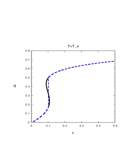
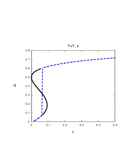
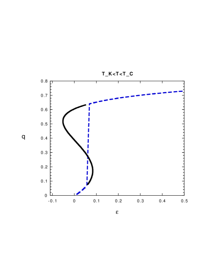
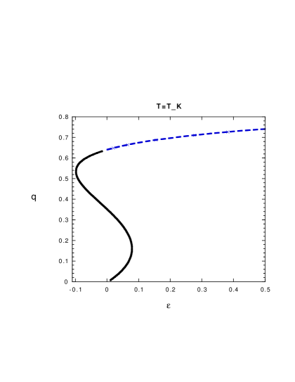
Figure 1.7: (From [41]; $T_{c}$ corresponds to $T_{d}$) Sketch of the function $q(\epsilon)$ in short range system (dashed line). A first order transition happens at $\epsilon_{c}(T)>0$ for $T>T_{K}$; at $T_{K}$, $\epsilon_{c}(T_{K})=0$. The correlated phase is metastable for $\epsilon<\epsilon_{c}(T)$ and follows approximately the mean field behavior (full line). For $T\sim T_{d}$ the metastability limit of the correlated phase is around $\epsilon=0$ and the complexity cannot be defined.

An ambiguity in the definition of $\Sigma(T)$ is present because the function $q(\epsilon)$ below $\epsilon_{c}$ (slightly) depends on the time scale and in general on the history of the system. However one can reasonably expect (relying on similar results obtained for Ising models, see e.g. [30, 51]) that the ambiguity is of the order of $\exp[-(\epsilon_{c}-\epsilon)^{-1}]$ for $\epsilon_{c}\gtrsim\epsilon$ so it becomes smaller and smaller on approaching $T_{K}$. Close to $T_{d}$ the ambiguity becomes very large and $\Sigma(T)$ cannot be properly defined in short range systems.

1.4.3 A first principles computation of the surface tension

A way to compute the free energy barrier for nucleation $\Delta F(T)$ using again the two–replica potential $V(q,T)$ has been recently proposed [46, 47]. Indeed, the potential $V(q,T)$ allows to realize the situation considered in section 1.4.1 in a way that is suitable for analytical computations.

The configuration $\sigma$ is a reference (frozen) configuration that belongs to an equilibrium state at temperature $T$. The configuration $\tau$ is constrained to have a fixed overlap $q$ with $\sigma$, so if $q=q(T)$ it belongs to the same state. Consider now a system with long but finite range interactions, whose scale is $1/\gamma$, $\gamma\sim 0$, enclosed in a volume $V=N\gamma^{-d}$, $N\rightarrow\infty$, i.e. the thermodynamic limit is taken at the beginning of the calculation. Consider an adimensional space variable $x$ obtained rescaling the space by $\gamma$, i.e. $\int d^{d}x=N$. We can define a local overlap $q(x)$ averaging the overlap over a large volume of linear dimension smaller than $1/\gamma$, and consider the potential $V[q(x),T]$ as a functional of the local overlap $q(x)$. A configuration $\tau$ such that

$$\begin{cases}&q(x)=q(T)\hskip 30.0pt\text{for}\,|x|\rightarrow\infty\ ,\\ &q(x)\sim 0\hskip 45.0pt\text{for}\,x=0\ ,\end{cases}$$ (1.58)

is in the same state of $\sigma$ outside some bubble of radius $R$ and is in another state inside the bubble. The quantity $\Delta F(T)=V[q(x),T]-V(q(T),T)$ represents exactly the free energy cost of this configuration with respect to the configuration in which the two replicas are in the same state in all the points of the space, so it is exactly the free energy barrier defined in section 1.4.1. The overlap profile $q(x)$ has to be determined by minimizing $V[q(x),T]$ with the boundary conditions (1.58) in order to find the most probable transition state for the nucleation [46, 47].

In systems with long but finite range (Kac spin glasses) it has been shown [45] that the potential $V[q(x),T]$ has a form very similar to the mean field one (1.35)

$$V[q(x),T]=-\frac{T\gamma^{d}}{N}\lim_{n\rightarrow 0}\lim_{m\rightarrow 1}\frac{1}{n}\frac{\partial}{\partial m}\overline{Z_{mn}[q(x)]}\ ,$$ (1.59)

where $Z_{mn}[q(x)]$ is the partition function of an $nm$-times replicated system such that in each $m\times m$ subblock the first replica has overlap $q(x)$ with the other $m-1$ replicas (as in mean field). The partition function has the form

$$Z_{mn}[q(x)]=\int{\cal D}Q(x)e^{\frac{1}{\gamma^{d}}S[Q(x)]}\ ,$$ (1.60)

where the matrix $Q(x)$ respects the constraint above, i.e. it has a structure similar to (1.39), and the action $S[Q(x)]$ has the form

$$S[Q(x)]=\int d^{d}x\big{\{}K[Q(x)]+f[Q(x)]\big{\}}\ ,$$ (1.61)

with $K[Q(x)]$ a kinetic term, $K[Q(x)]\sim-\frac{\beta}{2}{\rm Tr}\,[\nabla Q(x)]^{2}$, and $f[Q(x)]$ a potential identical to the mean field one given in Eq. (1.37). The mean field potential then plays the role of a local potential in each volume $\sim\gamma^{-d}$, while the contributions due to space variations on a scale $1/\gamma$ are taken into account by the kinetic term.

For $\gamma\rightarrow 0$, if one looks to homogeneous solutions $Q(x)\equiv Q$, all the results of the mean field model are reproduced. To look for nonhomogeneous solution respecting the boundary conditions (1.58), an ansatz of the form (1.39) in each point $x$ has been proposed [46]; if the potential has to been minimized also w.r.t. $q(x)$, one can assume that $r=q$ in each point $x$ as in the homogeneous case. This is the simplest possible ansatz and one obtains

$$V[q(x),T]=\frac{1}{N}\int d^{d}x\left\{\frac{1}{2}[\nabla q(x)]^{2}+V(q(x),T)\right\}\ ,$$ (1.62)

where $V(q,T)$ is the mean field potential. Then the equation for $q(x)$ has the form

$$\nabla^{2}q(x)=\frac{dV}{dq}\ ,$$ (1.63)

and the boundary conditions (1.58) have to be imposed to the solution. If one is able to solve Eq. (1.63), substituting the solution ${\overline{q}}(x)$ into the potential one can compute the barrier $\Delta F(T)=V[{\overline{q}}(x),T]-V(q(T),T)$. Subtracting from the barrier the bulk contribution $-T\Sigma(T)R^{d}$, one gets an estimate of the surface tension. A typical profile of the solution and the corresponding surface tension are reported in Fig. 1.8.

Figure 1.8: (From [47]) A typical instanton profile (full line) close to $T_{K}$. In the inset, the surface tension as a function of the droplet size is reported.

However, an approximate solution is possible if one looks for spherical solutions $q(r)$ with $r=|x|$ and, in the limit of large radius $R$, approximates the Laplacian, close to the interface, with

$$\nabla^{2}q\sim\frac{d^{2}q}{dr^{2}}=\frac{dV}{dq}\ .$$ (1.64)

In this case the problem becomes planar so the radius of the droplet remains undetermined. For a given radius $R$ of the droplet, the bulk term${}^{\ref{nota1}}$ is simply $[V(q(T),T)-V(q,0)]R^{d}=-T\Sigma(T)R^{d}$. To estimate the surface tension, i.e. the contribution to the integral (1.62) due to the interface, note that the quantity $E=\frac{1}{2}\left(\frac{dq}{dr}\right)^{2}-V(q,T)$ is conserved and is equal, recalling that, for $r\rightarrow\infty$, $\frac{dq}{dr}\rightarrow 0$, to $V(q(T),T)$, so one has, for $r\sim R$,

$$\frac{dq}{dr}=\sqrt{2[V(q,T)-V(q(T),T)]}\ ,$$ (1.65)

and the contribution coming from the region $r\sim R$ to the barrier $V[q(x),T]-V(q(T),T)$ is, defining $r_{-}$ such that $V(q(r_{-}),T)=V(q(T),T)$,

$$\begin{split}R^{d-1}\int_{r_{-}}^{\infty}dr&\left\{\frac{1}{2}\left(\frac{dq}{dr}\right)^{2}+V(q,T)-V(q(T),T)\right\}=R^{d-1}\int_{r_{-}}^{\infty}dr\left(\frac{dq}{dr}\right)^{2}=\\ &R^{d-1}\int_{q_{-}}^{q(T)}dq\sqrt{2[V(q,T)-V(q(T),T)]}\ ,\end{split}$$ (1.66)

so we get the following expression for the surface tension [46]:

$$\Upsilon(T)=\int_{q_{-}}^{q(T)}dq\sqrt{2[V(q,T)-V(q(T),T)]}\ .$$ (1.67)

As the difference $q(T)-q_{-}$ is always of order $1$, the surface tension scales as

$$\Upsilon(T)\sim\sqrt{V(q_{max},T)-V(q(T),T)}$$ (1.68)

and is finite at $T_{K}$. The outcome of the simplest instanton calculation is that $\theta=d-1$ and $\Upsilon(T_{K})\neq 0$. This leads to the scalings (1.57).

It has been recently found that a more refined calculation that includes replica symmetry breaking at the interface reduces the surface tension; from this observation an argument that leads to $\theta=d/2$ has been proposed. However, a detailed theory is still missing.

Chapter 2 The ideal glass transition of Hard Spheres

2.1 Introduction

The question whether a liquid of identical Hard Spheres undergoes a glass transition upon densification is still open, see e.g. [52, 53, 54, 55]. It is interesting to apply the replica method to the Hard Spheres liquid, following what has been done for Lennard–Jones systems [15, 41, 49] in order to investigate the possibility of the existence of a Kauzmann transition.

In an Hard Sphere system, on increasing the density, and if crystallization is avoided, one can access the metastable region of the phase diagram above the freezing packing fraction $\varphi_{f}=0.494$, where $\varphi=\frac{N\pi D^{3}}{6V}$, $D$ is the Hard Sphere diameter, $N$ is the number of particles and $V$ is the volume of the container. In this region the dynamics of the liquid becomes slower and slower on increasing the density. The particles are “caged” by their neighbors, and the dynamics separates into a fast rattling inside the cage and slow rearrangements of the cages. The typical time scale of these rearrangements increase very fast around $\varphi_{g}\sim 0.56$ and many authors reported the observation of a glass transition at these values of density [25, 26]. Note that the Kauzmann density is expected to be larger than the experimental glass transition density, as at $\varphi_{K}$ the relaxation time is expected to diverge so that the system freezes in a metastable state, on the experimental time scale, for a density $\varphi_{g}$ smaller than $\varphi_{K}$.

A related problem is the study of dense amorphous packings of Hard Spheres. Dense amorphous packings are relevant in the study of colloidal suspensions, granular matter, powders, etc. and have been widely studied in the literature [59, 60, 61, 62, 63, 64, 65, 66]. The metastable states of the Hard Sphere liquid provide examples of such packings: when the system freezes in one of these states, if one is still able to increase the density in order to reduce the size of the cages to zero (for example by shaking the container [60, 61] or using suitable computer algorithms [62, 63, 66]), a random close packed state is reached. The problem of which is the maximum value of density $\varphi_{c}$ that can be reached applying this kind of procedures has been tackled using a lot of different techniques, usually finding values of $\varphi_{c}$ in the range $0.62\div 0.67$. Another interesting problem is to estimate the mean coordination number $z$, i.e. the mean number of contacts between a sphere and its neighbors, in the random close packed states. Many studies addressed this question usually finding values of $z\sim 6$.

Few estimates of the configurational entropy for Hard Spheres are currently available [54, 57] and indicate a value of $\varphi_{K}$ in the range $0.58\div 0.62$. These estimates were obtained following numerical procedures already succesfully applied in Lennard–Jones systems [49, 56] or the method described in section 1.4.2; for the Lennard–Jones liquid the results compare well with the theoretical predictions of the replica theory [41, 49]. A tentative replica study of the Hard Spheres glass transition, based on the potential method described in section 1.3.2, can be found in [58], where a good estimate of $\varphi_{K}\sim 0.62$ was obtained. However, the configurational entropy computed in [58] is two orders of magnitude smaller than the one found in numerical simulations. This negative results is probably due to some technical problem in the assumptions of [58].

For technical reasons the real replica method (see section 1.3.1) of [15, 37, 41, 49, 67], that gives very good results for Lennard–Jones systems, cannot be extended straightforwardly to the case of Hard Spheres; indeed at some stage is was assumed that the vibrations around the equilibrium positions were harmonic in a first approximation. This approximation is not bad for soft potentials, but it clearly makes no sense for hard spheres.

In this chapter a way to adapt the replica method of [15] to the case of the Hard Sphere liquid, and in general of potentials such that the pair distribution function $g(r)$ shows discontinuities, will be developed. This allows to compute from first principles the configurational entropy of the liquid as well as the thermodynamic properties of the glass and the random close packing density. A very good estimate of the configurational entropy, that agrees well with the recent numerical simulations of [54, 57], a Kauzmann density in the range $0.58\div 0.62$ (depending on the equation of state we use to describe the liquid state), and a random close packing density in the range $0.64\div 0.67$, are found. Moreover, the mean coordination number in the amorphous packed states is found to be $z=6$ irrespective of the equation of state used for the liquid, in very good agreement with the result of numerical simulations [62, 63, 66].

2.2 The molecular liquid

The starting point of the real replica method described in section 1.3.1 is the free energy of a system of $m$ copies of the original liquid constrained to be in the same metastable state. This means that each atom of a given replica is close to an atom of each of the other $m-1$ replicas, i.e. , the liquid is made of molecules of $m$ atoms, each belonging to a different replica of the original system. In other words the atoms of different replicas stay in the same cage. The problem is then to compute the free energy of a molecular liquid where each molecule is made of $m$ atoms. The $m$ atoms are kept close one to each other by a small inter-replica coupling that is switched off at the end of the calculation, while each atom interacts with all the other atoms of the same replica via the original pair potential. This problem can be tackled by mean of the HNC integral equations [68].

2.2.1 HNC free energy

The traditional HNC approximation can be naturally extended to the case where particles have internal degrees of freedom and also to the replica approach where one has molecules composed by $m$ atoms.

Let $x=\{{\underline{x}}_{1},\cdots,{\underline{x}}_{m}\}$, ${\underline{x}}_{a}\in\hbox{\msytw R}^{d}$ be the coordinate of a molecule in dimension $d$. The single-molecule density is

$$\rho(x)=\langle\sum_{i=1}^{N}\prod_{a=1}^{m}\delta({\underline{x}}_{ia}-{\underline{x}}_{a})\rangle\ ,$$ (2.1)

and the pair correlation is

$$\rho(x)g(x,y)\rho(y)=\langle\sum_{i,j}^{1,N}\prod_{a=1}^{m}\delta({\underline{x}}_{ia}-{\underline{x}}_{a})\prod_{b=1}^{m}\delta({\underline{x}}_{jb}-{\underline{y}}_{b})\rangle\ .$$ (2.2)

Define also $h(x,y)=g(x,y)-1$. The interaction potential between two molecules is $v(x,y)=\sum_{a}v(|{\underline{x}}_{a}-{\underline{y}}_{a}|)$.

The HNC free energy is given by [15, 68]

$$\begin{split}\beta\Psi[\rho(x),g(x,y)]&=\frac{1}{2}\int dxdy\,\rho(x)\rho(y)\big{[}g(x,y)\log g(x,y)-g(x,y)+1+\beta v(x,y)g(x,y)\big{]}\\ &+\int dx\rho(x)\big{[}\log\rho(x)-1\big{]}+\frac{1}{2}\sum_{n\geq 3}\frac{(-1)^{n}}{n}{\rm Tr}\,[h\rho]^{n}\ ,\end{split}$$ (2.3)

where

$${\rm Tr}\,[h\rho]^{n}=\int dx_{1}\cdots dx_{n}h(x_{1},x_{2})\rho(x_{2})h(x_{2},x_{3})\rho(x_{3})\cdots h(x_{n-1},x_{n})\rho(x_{n})h(x_{n},x_{1})\rho(x_{1})\ .$$ (2.4)

For Hard Spheres the potential term vanishes, $\int dxdy\,\rho(x)\rho(y)g(x,y)v(x,y)\equiv 0$, so the reduced free energy $\beta\Psi$ will not depend on the temperature in all the following equations. Similarly, all the free energy functions that will be consider below do not depend on the temperature once multiplied by $\beta$. In principle one could stick to $\beta=1$ and slightly simplify the formulae. However, it is useful to keep explicitly $\beta$, in order to conform to the standard notation for soft spheres (or for hard spheres with an extra potential).

Differentiation w.r.t $g(x,y)$ leads to the HNC equation:

$$\log g(x,y)+\beta v(x,y)=h(x,y)-c(x,y)\ ,$$ (2.5)

having defined $c(x,y)$ from

$$h(x,y)=c(x,y)+\int dz\,c(x,z)\rho(z)h(z,y)\ .$$ (2.6)

The free energy (per particle) of the system is given by

$$\begin{split}&\phi(m,T)=\frac{1}{Nm}\min_{\rho(x),g(x,y)}\Psi[\rho(x),g(x,y)]\ ,\\ &\Phi(m,T)=m\phi(m,T)\ ,\end{split}$$ (2.7)

and once the latter is known one can compute the free energy of the states and the complexity using Eq.s (1.20).

2.2.2 Single molecule density

The solution of the previous equations for generic $m$ is a very complex problem (it is already rather difficult for $m=2$). Some kind of ansatz is needed to simplify the computation, that may become terribly complicated.

The single molecule density encodes the information about the inter-replica coupling that keeps all the replicas in the same state. One can assume that this arbitrarily small coupling has already been switched off, with the main effect of building molecules of $m$ atoms vibrating around the center of mass ${\underline{X}}\in\hbox{\msytw R}^{d}$ of the molecule with a certain “cage radius” $A$. The simplest ansatz for $\rho(x)$ is then [15]

$$\rho(x)=\widehat{\rho}\int d{\underline{X}}\prod_{a}\rho({\underline{x}}_{a}-{\underline{X}})\ ,\hskip 10.0pt\int d{\underline{u}}\,\rho({\underline{u}})=1\ ,$$ (2.8)

with

$$\rho({\underline{u}})=\frac{e^{-\frac{u^{2}}{2A}}}{(\sqrt{2\pi A})^{d}}\ ,$$ (2.9)

and $\widehat{\rho}=V^{-1}\int dx\,\rho(x)$ the number density of molecules. With this choice it is easy to show that

$$\frac{1}{N}\int dx\,\rho(x)\big{[}\log\rho(x)-1\big{]}=\log\widehat{\rho}-1+\frac{d}{2}(1-m)\log(2\pi A)-\frac{d}{2}\log m+\frac{d}{2}(1-m)\ .$$ (2.10)

2.2.3 Pair correlation

As the information about the inter-replica coupling is already encoded in $\rho(x)$, a reasonable ansatz for $g(x,y)$ is:

$$g(x,y)=\prod_{a}g(|{\underline{x}}_{a}-{\underline{y}}_{a}|)\ ,$$ (2.11)

where $g(r)$ is rotationally invariant because so is the interaction potential. It is useful to define $G(r)\equiv[g(r)]^{m}$. Using the ansatz above, it is easy to rewrite the free energy (2.3) as follows:

$$\begin{split}\beta\Psi&=\frac{\widehat{\rho}N}{2}\int d{\underline{r}}\,\big{\{}m[F_{0}(r)]^{m-1}F_{1}(r)-[F_{0}(r)]^{m}+1+m[F_{0}(r)]^{m-1}F_{v}(r)\big{\}}\\ &+\int dx\,\rho(x)\big{[}\log\rho(x)-1\big{]}+\frac{1}{2}\sum_{n\geq 3}\frac{(-1)^{n}}{n}{\rm Tr}\,[h\rho]^{n}\ ,\end{split}$$ (2.12)

where

$$\begin{split}&F_{p}(|{\underline{r}}|)=\int d{\underline{u}}d{\underline{v}}\,\rho({\underline{u}})\rho({\underline{v}})\,g(|{\underline{r}}+{\underline{u}}-{\underline{v}}|)[\log g(|{\underline{r}}+{\underline{u}}-{\underline{v}}|)]^{p}\ ,\\ &F_{v}(|{\underline{r}}|)=\int d{\underline{u}}d{\underline{v}}\,\rho({\underline{u}})\rho({\underline{v}})\,g(|{\underline{r}}+{\underline{u}}-{\underline{v}}|)\beta v(|{\underline{r}}+{\underline{u}}-{\underline{v}}|)\ .\end{split}$$ (2.13)

Note that as $g(r)$ and $v(r)$ are rotationally invariant, so are $F_{p}(r)$ and $F_{v}(r)$. If $\rho({\underline{u}})$ is given by Eq. (2.9), one gets

$$F(|{\underline{r}}|)=\int d{\underline{u}}\,\frac{e^{-\frac{u^{2}}{4A}}}{(\sqrt{4\pi A})^{d}}f(|{\underline{r}}+{\underline{u}}|)\ ,$$ (2.14)

where $f(r)\in\{g(r),\,g(r)\log g(r),\,g(r)\beta v(r)\}$. For Hard Spheres $F_{v}\equiv 0$.

2.3 Small cage expansion

The strategy of [15] was to expand the HNC free energy in a power series of the cage radius $A$, assuming that the latter is small close to the glass transition. The expansion is carried out easily if the pair potential $v(r)$ and the pair correlation $g(r)$ are analytic functions of $r$. However this is not the case for Hard Spheres, as $g(r)$ vanishes for $r<D$ and has a discontinuity in $r=D$, so the formulae of [15] for the power series expansion of $\Psi$ cannot be applied to our system.

It is crucial to realize that, independently from any approximation, in the limit $A\rightarrow 0$, the partition function becomes (neglecting a trivial factor) the partition function of a single atom at an effective temperature given by $\beta_{eff}=\beta m$. In the case of Hard Spheres, where there is no dependence on the temperature, the change in temperature is irrelevant.

In [15] it was shown that the first term of the expansion is proportional to $A$ if $g(r)$ is differentiable. It will be shown in the following that, in the case of Hard Spheres, the presence of a jump in $g(r)$ produces terms $O(\sqrt{A})$ in the expansion. At first order one can focus on these terms neglecting all the contributions of higher order in $\sqrt{A}$. This means that one can neglect all the contributions coming from the regions where $g(r)$ is differentiable and concentrate only on what happens around $r=D$.

2.3.1 Expansion of $F_{0}(r)$

The contribution one wants to estimate comes from the discontinuity of $g(r)$ in $r=D$. Thus to compute this correction the form of $g(r)$ away from the singularity is irrelevant and one can use the simplest possible form of $g(r)$.

It is convenient to discuss first the expansion of $F_{0}(r)$ in $d=1$. The simplest possible form of $g(r)$ is

$$g(r)=\theta(r-D)[1+(y-1)e^{-\mu(r-D)}]\ ;$$ (2.15)

the amplitude of the jump of $g(r)$ in $r=D$ is given by $y$. Remember that ${\underline{r}}\in\hbox{\msytw R}$ and $r=|{\underline{r}}|\in\hbox{\msytw R}^{+}$. As the functions $F_{0}$ and $g$ are even in ${\underline{r}}$, one can write

$$\int_{-\infty}^{\infty}d{\underline{r}}[F_{0}({\underline{r}})^{m}-g({\underline{r}})^{m}]=2\int_{0}^{\infty}dr[F_{0}(r)^{m}-g(r)^{m}]\ .$$ (2.16)

Defining

$$\begin{split}&\text{erf}(t)\equiv\frac{2}{\sqrt{\pi}}\int_{0}^{t}dx\,e^{-x^{2}}\ ,\\ &\Theta(t)=\frac{1}{2}[1+\text{erf}(t)]\ ,\end{split}$$ (2.17)

these functions play the role of “smoothed” sign and $\theta$-function respectively; note also that the function $\Theta(t)$ goes to $0$ as $e^{-t^{2}}$ for $t\rightarrow-\infty$. Then

$$\int_{-\infty}^{\infty}du\,\frac{e^{-\frac{u^{2}}{4A}}}{\sqrt{4\pi A}}\,\theta(r+u-D)=\frac{1}{2}\left[1+\text{erf}\left(\frac{r-D}{\sqrt{4A}}\right)\right]\equiv\Theta\left(\frac{r-D}{\sqrt{4A}}\right)\ ,$$ (2.18)

and

$$\begin{split}F_{0}(r)&=\Theta\left(\frac{r-D}{\sqrt{4A}}\right)+\Theta\left(-\frac{r+D}{\sqrt{4A}}\right)+(y-1)e^{A\mu^{2}}\Big{\{}e^{-\mu(r-D)}\Theta\left(\frac{r-D-2A\mu}{\sqrt{4A}}\right)\\ &+e^{\mu(r+D)}\Theta\left(-\frac{r+D+2A\mu}{\sqrt{4A}}\right)\Big{\}}\ .\end{split}$$ (2.19)

As $r\geq 0$ one can neglect the terms proportional to $\Theta\left(-\frac{r+D}{\sqrt{4A}}\right)$ in Eq. (2.19), that give a contribution of order $\exp(-D^{2}/A)$ for $A\rightarrow 0$. Defining the reduced variable $t=(r-D)/\sqrt{4A}$:

$$\begin{split}g(t)&=\theta(t)[1+(y-1)e^{-\mu 2\sqrt{A}t}]\ ,\\ F_{0}(t)&=\Theta(t)+(y-1)e^{-\mu 2\sqrt{A}t}\,e^{A\mu^{2}}\Theta(t+\mu\sqrt{A})\ ,\end{split}$$ (2.20)

and Eq. (2.16) becomes

$$\int_{0}^{\infty}dr[F_{0}(r)^{m}-g(r)^{m}]=2\sqrt{A}\int_{-\frac{D}{\sqrt{4A}}}^{\infty}dt[F_{0}(t)^{m}-g(t)^{m}]\equiv 2\sqrt{A}Q(A)\ .$$ (2.21)

If the function $Q(A)$ has a finite limit $Q(0)$ for $A\rightarrow 0$ one has $Q(A)=Q(0)+o(1)$ and the leading correction to the free energy is $O(\sqrt{A}Q(0))$. The limit for $A\rightarrow 0$ of $Q(A)$ is formally given by

$$Q(0)=y^{m}\int_{-\infty}^{\infty}dt\,[\Theta(t)^{m}-\theta(t)^{m}]\equiv y^{m}Q_{m}$$ (2.22)

where $y^{m}\equiv Y$ is the jump of $G(r)\equiv g(r)^{m}$ in $r=D$ and $Q_{m}\equiv\int_{-\infty}^{\infty}dt\,[\Theta(t)^{m}-\theta(t)^{m}]$. It is easy to show that $Q_{m}$ is a finite and smooth function of $m$ for $m\neq 0$, that

$$\begin{split}&Q_{m}=(1-m)Q_{0}+O[(m-1)^{2}]\ ,\\ &Q_{0}=-\int_{-\infty}^{\infty}dt\,\Theta(t)\log\Theta(t)\sim 0.638\ ,\end{split}$$ (2.23)

and that $Q_{m}$ diverges as $Q_{m}\sim\sqrt{\pi/4m}$ for $m\rightarrow 0$. Finally, recalling that $G(r)=[g(r)]^{m}$,

$$\frac{1}{2}\int d{\underline{r}}\,F_{0}(r)^{m}=\frac{1}{2}\int d{\underline{r}}\,G(r)+2\sqrt{A}YQ_{m}\ .$$ (2.24)

In dimension $d>1$, recalling that $F_{0}(r)$ and $G(r)$ are both rotationally invariant, one has

$$\int d{\underline{r}}\,[F_{0}(r)^{m}-G(r)^{m}]=\Omega_{d}\int_{0}^{\infty}dr\,r^{d-1}\,[F_{0}(r)^{m}-G(r)^{m}]\ ,$$ (2.25)

where $\Omega_{d}$ is the solid angle in $d$ dimension, $\Omega_{d}=2\pi^{d/2}/\Gamma(d/2)$. The function $F_{0}(r)$ can be written as

$$F_{0}(r)=\int d{\underline{u}}\,\frac{e^{-\frac{u^{2}}{4A}}}{(\sqrt{4\pi A})^{d}}g(|r\widehat{i}+{\underline{u}}|)\ ,$$ (2.26)

where $\widehat{i}$ is the unit vector e.g. of the first direction in $\hbox{\msytw R}^{d}$. For small $\sqrt{A}$, the $u$ are small too. The function $g(|r\widehat{i}+{\underline{u}}|)$ is differentiable along the directions orthogonal to $\widehat{i}$. Expanding in series of $u_{\mu}$, $\mu\neq 1$, at fixed $u_{1}$, one sees that the integration over these variables gives a contribution $O(A)$, so

$$F_{0}(r)=\int_{-\infty}^{\infty}du_{1}\,\frac{e^{-\frac{u_{1}^{2}}{4A}}}{\sqrt{4\pi A}}g(r+u_{1})+O(A)\ ,$$ (2.27)

as in the one dimensional case. The function $F_{0}(r)^{m}-G(r)^{m}$ is large only for $r-D\sim\sqrt{A}$ so at the lowest order one can replace $r^{d-1}$ with $D^{d-1}$ in Eq. (2.25), and obtains

$$\int d{\underline{r}}\,[F_{0}(r)^{m}-G(r)^{m}]=\Omega_{d}D^{d-1}\int_{0}^{\infty}dr\,[F_{0}(r)^{m}-G(r)^{m}]\ .$$ (2.28)

The last integral, with $F_{0}(r)$ given by Eq. (2.27) is the same as in $d=1$, so

$$\frac{1}{2}\int d{\underline{r}}\,F_{0}(r)^{m}=\frac{1}{2}\int d{\underline{r}}\,G(r)+\sqrt{A}Y\Sigma_{d}(D)Q_{m}\ ,$$ (2.29)

where $\Sigma_{d}(D)$ is the surface of a $d$-dimensional sphere of radius $D$, $\Sigma_{d}(D)=\Omega_{d}D^{d-1}$. This result can be formally written as

$$F_{0}(r)^{m}\sim G(r)+2\sqrt{A}YQ_{m}\delta(|r|-D)\equiv G(r)+Q_{0}(r)$$ (2.30)

as the correction comes only from the region close to the singularity of $g(r)$, $r-D\sim\sqrt{A}$.

2.3.2 $G\log G$-term

The correction coming from the term $\int dr\,mF_{0}(r)^{m-1}F_{1}(r)$ will now be estimated. Using the same argument as in the previous subsection, one can restrict to $d=1$. Note first that $F_{0}(r)$, for $|r-D|\sim\sqrt{A}$, has the form

$$F_{0}(r)=y\,\Theta\left(\frac{r-D}{\sqrt{4A}}\right)+o(\sqrt{A})\ ,$$ (2.31)

where $y$ is the jump of the function $g(r)$ in $r=D$. Similarly, $F_{1}(r)$ has the form

$$F_{1}(r)=\begin{cases}g(r)\log g(r)+O(A)\ ,\hskip 33.0pt|r-D|\gg\sqrt{A}\ ,\\ y\log y\,\Theta\left(\frac{r-D}{\sqrt{4A}}\right)+o(\sqrt{A})\ ,\hskip 10.0pt|r-D|\sim\sqrt{A}\ .\end{cases}$$ (2.32)

The integral

$$\int_{0}^{\infty}dr[mF_{0}(r)^{m-1}F_{1}(r)-mg(r)^{m}\log g(r)]$$ (2.33)

has then two contributions: the first comes from the region $|r-D|\gg\sqrt{A}$ and is of order $A$ as if the function $g(r)$ were continuous. The other comes from the region $|r-D|\sim\sqrt{A}$ and is of order $\sqrt{A}$ as in the previous case. To estimate the latter one can use again the reduced variable $t$ and approximate $F_{1}(t)\sim y\log y\,\Theta(t)$, $F_{0}(t)\sim y\,\Theta(t)$. Then

$$\int_{0}^{\infty}dr[mF_{0}(r)^{m-1}F_{1}(r)-mg(r)^{m}\log g(r)]=Y\log Y\,2\sqrt{A}Q_{m}+o(\sqrt{A})\ ,$$ (2.34)

in $d=1$ and finally, in any dimension $d$,

$$\frac{1}{2}\int d{\underline{r}}\,mF_{0}(r)^{m-1}F_{1}(r)=\frac{1}{2}\int d{\underline{r}}\,G(r)\log G(r)+\sqrt{A}Y\log Y\,\Sigma_{d}(D)Q_{m}\ .$$ (2.35)

2.3.3 Interaction term

Substituting Eq. (2.8) in the last term of the HNC free energy one obtains

$${\rm Tr}\,[h\rho]^{n}=\widehat{\rho}^{n}\int d{\underline{X}}_{1}\cdots d{\underline{X}}_{n}\int du_{1}\cdots du_{n}\rho(u_{1})\cdots\rho(u_{n})h({\underline{X}}_{1}-{\underline{X}}_{2},u_{1}-u_{2})\cdots h({\underline{X}}_{n}-{\underline{X}}_{1},u_{n}-u_{1})\ ,$$ (2.36)

where $h(X,u)=\prod_{a=1}^{m}g(X+u_{a})-1$ and $\rho(u)=\prod_{a=1}^{m}\rho({\underline{u}}_{a})$ with $\rho({\underline{u}})$ given by Eq. (2.9).

The correction $O(\sqrt{A})$ to this integral comes from the regions where $|X_{i}-X_{i+1}|=D+O(\sqrt{A})$ for some $i=1,\cdots,n$. In these regions the functions $h$ such that their arguments are not close to the singularity can be expanded in a power series in $u$, the correction being $O(A)$ [15]. Thus one can write, defining $H(r)=G(r)-1$:

$$\begin{split}\widehat{\rho}^{-n}{\rm Tr}\,[h\rho]^{n}&=\int d{\underline{X}}_{1}\cdots d{\underline{X}}_{n}H({\underline{X}}_{1}-{\underline{X}}_{2})\cdots H({\underline{X}}_{n}-{\underline{X}}_{1})+n\int d{\underline{X}}_{1}\cdots d{\underline{X}}_{n}\int du_{1}du_{2}\times\\ \times\rho(u_{1})&\rho(u_{2})\big{[}h({\underline{X}}_{1}-{\underline{X}}_{2},u_{1}-u_{2})-H({\underline{X}}_{1}-{\underline{X}}_{2})\big{]}H({\underline{X}}_{2}-{\underline{X}}_{3})\cdots H({\underline{X}}_{n}-{\underline{X}}_{1})=\\ &\int d{\underline{X}}_{1}\cdots d{\underline{X}}_{n}H({\underline{X}}_{1}-{\underline{X}}_{2})\cdots H({\underline{X}}_{n}-{\underline{X}}_{1})\\ &+n\int d{\underline{X}}_{1}\cdots d{\underline{X}}_{n}Q_{0}({\underline{X}}_{1}-{\underline{X}}_{2})H({\underline{X}}_{2}-{\underline{X}}_{3})\cdots H({\underline{X}}_{n}-{\underline{X}}_{1})\ ,\end{split}$$ (2.37)

where in the last step Eq. (2.30) has been used:

$$\int du_{1}du_{2}\,\rho(u_{1})\rho(u_{2})\big{[}h(r,u_{1}-u_{2})-H(r)\big{]}=F_{0}(r)^{m}-G(r)=Q_{0}(r)\ .$$ (2.38)

Collecting all the terms with different $n$ one has

$$\begin{split}\frac{1}{2}\sum_{n\geq 3}\frac{(-1)^{n}}{n}{\rm Tr}\,[h\rho]^{n}&\sim\frac{1}{2}\sum_{n\geq 3}\frac{(-1)^{n}}{n}\widehat{\rho}^{n}{\rm Tr}\,H^{n}+\frac{\widehat{\rho}^{3}}{2}\int d{\underline{X}}_{1}d{\underline{X}}_{2}d{\underline{X}}_{3}Q_{0}({\underline{X}}_{1}-{\underline{X}}_{2})H({\underline{X}}_{2}-{\underline{X}}_{3})\times\\ &\times\sum_{n\geq 3}(-1)^{n}\widehat{\rho}^{n-3}\int d{\underline{X}}_{4}\cdots d{\underline{X}}_{n}H({\underline{X}}_{3}-{\underline{X}}_{4})\cdots H({\underline{X}}_{n}-{\underline{X}}_{1})=\\ =\frac{1}{2}\sum_{n\geq 3}\frac{(-1)^{n}}{n}&\widehat{\rho}^{n}{\rm Tr}\,H^{n}-\frac{\widehat{\rho}^{3}}{2}\int d{\underline{X}}_{1}d{\underline{X}}_{2}d{\underline{X}}_{3}Q_{0}({\underline{X}}_{1}-{\underline{X}}_{2})H({\underline{X}}_{2}-{\underline{X}}_{3})C({\underline{X}}_{3}-{\underline{X}}_{1})\ .\end{split}$$ (2.39)

Substituting the expression of $Q_{0}(r)$ and recalling that from the definition of $C({\underline{X}})$ one has

$$\widehat{\rho}\int d{\underline{Z}}H({\underline{X}}-{\underline{Z}})C({\underline{Z}}-{\underline{Y}})=H({\underline{X}}-{\underline{Y}})-C({\underline{X}}-{\underline{Y}})\ ,$$ (2.40)

the following result is obtained (in any dimension $d$):

$$\frac{1}{2}\sum_{n\geq 3}\frac{(-1)^{n}}{n}{\rm Tr}\,[h\rho]^{n}=\frac{1}{2}\sum_{n\geq 3}\frac{(-1)^{n}}{n}\widehat{\rho}^{n}{\rm Tr}\,H^{n}-N\widehat{\rho}Q_{m}\sqrt{A}y\Sigma_{d}(D)[H(D)-C(D)]\ .$$ (2.41)

2.4 First order free energy

Figure 2.1: The equilibrium complexity $\Sigma(\varphi)$ as a function of the packing fraction.

Substituting Eq.s (2.29), (2.35) and (2.41) in Eq. (2.12) one obtains the following expression for the HNC free energy at first order in $\sqrt{A}$:

$$\begin{split}\beta F&=\frac{\beta\Psi}{N}=\beta F_{0}(A)+\beta F_{eq}[G(r)]+\beta\Delta F[A,G(r)]\ ,\\ \beta F_{eq}&=\frac{\widehat{\rho}}{2}\int d^{d}r\,\big{[}G(r)\log G(r)-G(r)+1\big{]}+\log\widehat{\rho}-1\\ &+\frac{1}{2\widehat{\rho}}\int\frac{d^{d}k}{(2\pi)^{d}}\left[-\log[1+\widehat{H}(k)]+\widehat{H}(k)-\frac{1}{2}\widehat{H}(k)^{2}\right]\ ,\\ \beta F_{0}&=\frac{d}{2}(1-m)\log(2\pi A)+\frac{d}{2}(1-m)-\frac{d}{2}\log m\ ,\\ \beta\Delta F&=\widehat{\rho}Q_{m}\sqrt{A}\Sigma_{d}(D)\,G(D)\big{[}\log G(D)-1-H(D)+C(D))\big{]}\ ,\end{split}$$ (2.42)

where $Q_{m}=Q_{0}(1-m)+o((m-1)^{2})$, $Q_{0}\sim 0.638$ and the Fourier transform has been defined as

$$\widehat{H}(k)=\widehat{\rho}\int dr\,e^{ikr}H(r)\ .$$ (2.43)

At the first order in $\sqrt{A}$ one only needs to know the function $G(r)$ determined by the optimization of the free energy at the zeroth order in $\sqrt{A}$, i.e. the usual free energy $F_{eq}[G(r)]$: it satisfies the HNC equation $\log G(r)=H(r)-C(r)$. Substituting this relation in $\beta\Delta F$ one simply obtains $\beta\Delta F=-\widehat{\rho}Q_{m}\sqrt{A}\Sigma_{d}(D)\,G(D)$.

The derivative w.r.t. $A$ leads to the following expression for the cage radius:

$$\sqrt{A^{*}}=\frac{1-m}{Q_{m}}\frac{d}{\widehat{\rho}\Sigma_{d}(D)G(D)}\ ,$$ (2.44)

which in $d=3$ becomes, defining again $Y=G(D)$:

$$\frac{\sqrt{A^{*}}}{D}=\frac{1-m}{Q_{m}}\frac{1}{8\,\varphi\,Y(\varphi)}\ ,$$ (2.45)

where $\varphi=\frac{\pi D^{3}\widehat{\rho}}{6}$ is the packing fraction. Substituting this result in $\beta\Delta F$ one has $\beta\Delta F(A^{*})=d(m-1)$.

Finally, the expression for the replicated free energy in $d=3$ is

$$\beta\Phi(m,\varphi)=\beta F_{eq}(\varphi)+\frac{3}{2}(1-m)\log[2\pi A^{*}(m)]+\frac{3}{2}(m-1)-\frac{3}{2}\log m\ .$$ (2.46)

Note that for Hard Spheres one has $\beta F_{eq}(\varphi)=-S(\varphi)$, $S$ being the total entropy of the liquid. Then

$$\begin{split}\beta f^{*}(&m,\varphi)=\frac{\partial\beta\Phi}{\partial m}=-\frac{3}{2}\log[2\pi A^{*}(m)]+\frac{3}{2}(1-m)\frac{d\log A^{*}(m)}{dm}+\frac{3}{2}\frac{m-1}{m}\ ,\\ \Sigma(m&,\varphi)=m\beta f^{*}-\beta\Phi=S(\varphi)-\frac{3}{2}\log[2\pi A^{*}(m)]+\frac{3m}{2}(1-m)\frac{d\log A^{*}(m)}{dm}+\frac{3}{2}\log m\ .\end{split}$$ (2.47)

For small enough density the system is in the liquid phase and $m$ is equal to 1. For $m=1$ one has:

$$\begin{split}&\frac{\sqrt{A^{*}(1)}}{D}=\frac{1}{8Q_{0}\,\varphi\,Y(\varphi)}\ ,\\ &S_{vib}(\varphi)\equiv-\beta f^{*}(1,\varphi)=\frac{3}{2}\log[2\pi A^{*}(1)]\ ,\\ &\Sigma(\varphi)=S(\varphi)-S_{vib}(\varphi)\ .\end{split}$$ (2.48)

This allows for a computation of $\Sigma(\varphi)$ once $S(\varphi)$ and $Y(\varphi)$ are known. Note that $1+4\varphi Y(\varphi)=\beta P/\rho=-\varphi\frac{\partial S}{\partial\varphi}$, so a model for $S(\varphi)$ (or $Y(\varphi)$) is enough to determine all the quantities of interest.

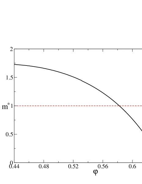
Figure 2.2: Phase diagram of the molecular liquid. For $m<m^{*}$ (full line) the system is in the liquid phase, for $m>m^{*}$ it is in the glass phase.

2.4.1 Results from the HNC free energy

The functions $S(\varphi)$ and $Y(\varphi)$ have been computed solving numerically the classical HNC equation for the Hard Sphere liquid up to $\varphi=0.65$. This allows to compute $\beta\Phi(\varphi,m)$ and gives access to all the thermodynamic quantities using Eq.s (2.47) and (2.48). In this section we discuss the results of this computation. The sphere diameter will be set to $D=1$ in the following.

Equilibrium complexity

The equilibrium complexity $\Sigma(\varphi)$ is given by Eq. (2.48). It is reported in Fig. 2.1. A complexity $\Sigma\sim 1$ is obtained as found in previous calculations in Lennard-Jones systems [15, 41, 49, 67], as well as in the numerical simulations [49, 56]. The complexity vanishes at $\varphi_{K}=0.582$, that is the ideal glass transition density –or Kauzmann density– predicted by the HNC equations.

Phase diagram in the $(\varphi,m)$ plane

As discussed above, it exists a value of $m$, $m^{*}(\varphi)$, such that for $m<m^{*}(\varphi)$ the system is in the liquid phase, and for $m>m^{*}(\varphi)$ is is in the glassy phase. It is the solution of $\Sigma(m,\varphi)=0$, where $\Sigma(m,\varphi)$ is given by Eq. (2.47). In Fig. 2.2 $m^{*}$ is reported as a function of $\varphi$. Clearly, $m^{*}=1$ at $\varphi=\varphi_{K}$ and $m^{*}<1$ for $\varphi>\varphi_{K}$. $m^{*}$ vanishes linearly at $\varphi_{c}=0.640$. As will be shown in the following, above this value of $\varphi$ the glassy state does not exist anymore.

Thermodynamic properties of the glass

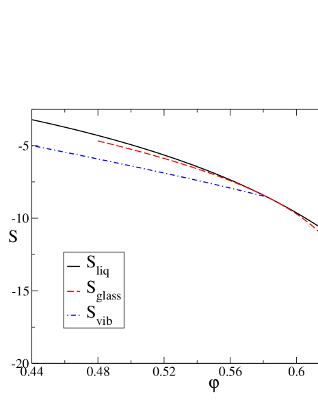
Figure 2.3: Entropy of the liquid (full line) and of the glass (dashed line). The two curves intersect at $\varphi_{K}=0.582$ where they are tangent and consequently the pressure is continuous at the glass transition. The entropy of the glass goes to $-\infty$ at $\varphi=\varphi_{c}=0.640$, so the glassy phase does not exist above $\varphi_{c}$. The dot–dashed line is the entropy of the equilibrium states of the liquid, $S_{vib}(\varphi)=S(\varphi)-\Sigma(\varphi)$.

The knowledge of the function $m^{*}(\varphi)$ allows to compute the entropy of the glass. Indeed, the free energy does not depend on $m$ in the whole glassy phase, and it is continuous along the line $m=m^{*}(\varphi)$, so the entropy of the glass is given by

$$S_{glass}(\varphi)=-\beta F_{glass}(\varphi)=-\frac{\beta\Phi(m^{*}(\varphi),\varphi)}{m^{*}(\varphi)}$$ (2.49)

This relation is true for $m^{*}<1$. Below $\varphi_{K}$ one has $m^{*}>1$ and the liquid phase is the stable one. Eq. (2.49) for $m^{*}>1$ gives the entropy of the lowest states in the free energy landscape (see below) and can be regarded as the analytic continuation of the glass entropy below $\varphi_{K}$. The reader should notice that the glass phase for $m^{*}>1$ does not have a simple physical meaning and the interesting part of the curves for the glass is in the region $\varphi>\varphi_{K}$.

In Fig. 2.3 the entropies of the liquid and the glass are reported as functions of the packing fraction. The glass phase becomes stable above $\varphi_{K}=0.582$; note that the entropy of the glass is smaller than the entropy of the liquid, i.e. its free energy is bigger than the free energy of the liquid. The same happens also in Lennard-Jones systems and in mean-field spin glass systems. However the physically relevant parts of the curves are the liquid one for $\varphi<\varphi_{K}$ and the glassy one for $\varphi>\varphi_{K}$.

The reduced pressure,

$$\frac{\beta P}{\rho}=-\varphi\frac{\partial S}{\partial\varphi}\ ,$$ (2.50)

is reported in Fig. 2.4.

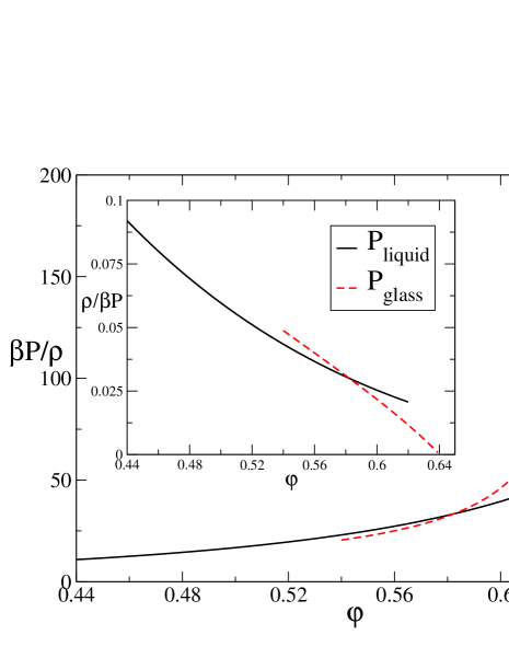
Figure 2.4: Reduced pressure $\beta P/\rho$ of the liquid and the glass as functions of the packing fraction. The pressure is continuous at $\varphi_{K}$. In the inset, the inverse reduced pressure is plotted; in the glass phase it is proportional to $\varphi_{c}-\varphi$.

It is continuous at $\varphi_{K}$ and the glass transition is a second order transition from the thermodynamical point of view. Note that the pressure in the glass phase is well described by a power law and it has a simple pole at $\varphi_{c}$:

$$\frac{\beta P_{glass}}{\rho}\propto\frac{1}{\varphi_{c}-\varphi}\ ,$$ (2.51)

as one can see from the inset of Fig. 2.4 where the inverse reduced pressure is plotted as a function of $\varphi$.

For $\varphi\rightarrow\varphi_{c}$ the pressure of the glass diverges and its compressibility $\chi=\frac{1}{\varphi}\frac{\partial\varphi}{\partial P}$ vanishes and consequently $\varphi_{c}$ is the maximum density allowed for a disordered state, i.e. it can be identified as the random close packing density. The value $\varphi_{c}=0.640$ is in very good agreement with the values reported in the literature. Note that the compressibility jumps downward on increasing $\varphi$ across $\varphi_{K}$, i.e. the compressibility of the glass is smaller than the compressibility of the liquid.

Cage radius

The cage radius is given as a function of $m$ in Eq. (2.45). In Fig. 2.5 the cage radius in the liquid phase, $\sqrt{A^{*}(1)}$, see Eq. (2.48), and the cage radius in the glass phase, defined as $\sqrt{A^{*}(m^{*})}$, are reported. As $Q_{m}\sim\sqrt{\pi/4m}$ for $m\sim 0$, the cage radius vanishes as $\sqrt{m^{*}}$ for $m^{*}\sim 0$, i.e. it is proportional to $\sqrt{\varphi_{c}-\varphi}$. The vanishing of the cage radius for $\varphi\rightarrow\varphi_{c}$ means that at $\varphi_{c}$ each sphere is in contact with its neighbors, that is consistent with the interpretation of $\varphi_{c}$ as the random close packing density.

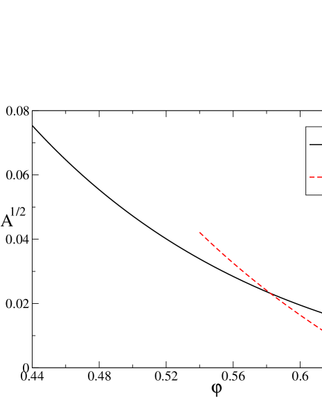
Figure 2.5: Cage radius $\sqrt{A}$ (in units of $D$) in the liquid and in the glass phase as function of $\varphi$.

Complexity of the metastable states

From the parametric plot of $\beta f^{*}(m,\varphi)$ and $\Sigma(m,\varphi)$ given in Eq. (2.47) by varying $m$, one can reconstruct the function $\Sigma(\beta f)$ for each value of the packing fraction. This function is reported in Fig. 2.6 for some values of $\varphi$ below and above $\varphi_{K}$. The function $\Sigma(\beta f)$ vanishes at a certain value $\beta f_{min}$, that is given by Eq. (2.49). The saddle-point equation that determines the free energy of the equilibrium states is, from Eq. (1.15),

$$\frac{d\Sigma(\beta f)}{d\beta f}=1\ .$$ (2.52)

From Fig. 2.6 it is clear that this equation has a solution $f^{*}>f_{min}$ for $\varphi<\varphi_{K}=0.582$. Above $\varphi_{K}$ Eq. (2.52) does not have a solution so the saddle point is simply $f^{*}=f_{min}$ and the systems goes in the glass state. In this sense, the free energy $f_{min}$ of the lowest states below $\varphi_{K}$ can be regarded as the analytic continuation of the free energy of the glass, see Fig. 2.3. The curves $\Sigma(\beta f)$ in Fig. 2.6 have been truncated arbitrarily at high $\beta f$. One should perform a consistency check to investigate where the higher free energy states become unstable (i.e. , to compute $f_{max}$). This is not trivial and is left for future work.

2.5 Correlation functions

The replica approach also allows the study of the pair distribution function $\tilde{g}(r)$ in the glass state. In principle a full computation would require the evaluation of the corrections proportional to $\sqrt{A}$ in the correlation functions of a molecule. However these terms will be neglected, as one can argue that they are small, and one can start again from the simple ansatz (2.8), (2.11) for the correlation function of the molecules, in which the information on the shape of the molecule is only encoded in the function $\rho(x)$; these corrections should be physically more relevant and interesting.

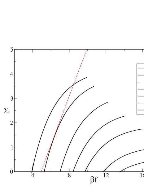
Figure 2.6: Complexity of the metastable states as a function of their free energy $\beta f$ for different values of $\varphi$. From left to right, $\varphi=0.45,0.5,0.55,0.58,0.6,0.62,0.63$. The curves are truncated arbitrarily at high $\beta f$. The dashed line has slope $1$.

As will be shown in the following, the correlation function of the spheres in the glass is very similar to the one in the liquid but develops an additional strong peak (that becomes a $\delta$-function at $\varphi_{c}$) around $r=D$. The integral of the latter peak is related to the average coordination number of the random close packings.

2.5.1 Expression of $\tilde{g}(r)$ in the glass phase

The following form for the pair distribution function of the molecular liquid was assumed in Eq.s (2.8) and (2.11):

$$\rho_{2}(x,y)=\rho(x)g(x,y)\rho(y)=\widehat{\rho}^{2}\int dXdY\prod_{a=1}^{m}\rho(x_{a}-X)g(|x_{a}-y_{a}|)\rho(y_{a}-Y)\ .$$ (2.53)

The pair correlation $\tilde{g}(r)$ of a single replica is obtained integrating over the coordinates of all the replicas but one:

$$\tilde{g}(|{\underline{x}}_{1}-{\underline{y}}_{1}|)=\widehat{\rho}^{-2}\int d{\underline{x}}_{2}\cdots d{\underline{x}}_{m}d{\underline{y}}_{2}\cdots d{\underline{y}}_{m}\rho_{2}(x,y)\ .$$ (2.54)

Using Eq. (2.53) one gets, with some simple changes of variable:

$$\tilde{g}(r)=g(r)\int d{\underline{u}}d{\underline{v}}\rho({\underline{u}})\rho({\underline{v}})F_{0}(|{\underline{r}}+{\underline{u}}-{\underline{v}}|)^{m-1}\ ,$$ (2.55)

where $F_{0}(r)$ is defined in Eq. (2.13). The HNC free energy is optimized by $g(r)=G(r)^{1/m}$, where $G(r)$ is the HNC pair correlation. Thus the following expression for the pair correlation of a single replica is obtained:

$$\begin{split}&\tilde{g}(r)=G(r)^{\frac{1}{m}}\int d{\underline{u}}\frac{e^{-\frac{u^{2}}{4A}}}{(\sqrt{4\pi A})^{d}}F_{0}(|{\underline{r}}+{\underline{u}}|)^{m-1}\ ,\\ &F_{0}(r)=\int d{\underline{u}}\frac{e^{-\frac{u^{2}}{4A}}}{(\sqrt{4\pi A})^{d}}G(|{\underline{r}}+{\underline{u}}|)^{\frac{1}{m}}\ .\end{split}$$ (2.56)

For $m=1$, i.e. in the liquid phase, this function is trivially equal to $G(r)$. This is not the case in the glass phase where $m<1$.

2.5.2 Small cage expansion of the correlation function

To expand Eq. (2.56) for small $A$, note first that, if $r\neq D$, the function $g(r+u)$ can be expanded in powers of $u$, and the first correction to $\tilde{g}(r)$ is of order $A$. Then, as before, one can concentrate only on what happens around $r=D$. As already discussed in section 2.3, around $r=D$ one has, as in Eq. (2.31), $G(r)\sim Y\theta(r-D)$ and

$$F_{0}(r)\sim Y^{\frac{1}{m}}\Theta\left(\frac{r-D}{\sqrt{4A}}\right)\ ,$$ (2.57)

and Eq. (2.56) becomes

$$\tilde{g}(r)=Y\theta(r-D)\int d{\underline{u}}\frac{e^{-\frac{u^{2}}{4A}}}{(\sqrt{4\pi A})^{d}}\Theta\left(\frac{|{\underline{r}}+{\underline{u}}|-D}{\sqrt{4A}}\right)^{m-1}\ .$$ (2.58)

Applying the same argument used in section 2.3 when studying the function $F_{0}(r)$ in dimension $d>1$, it can be shown that the integration over the coordinates $u_{\mu}$, $\mu\neq 1$, gives a contribution $O(A)$. Then, in any dimension $d$:

$$\begin{split}\tilde{g}(r)&\sim Y\theta(r-D)\int_{-\infty}^{\infty}du\frac{e^{-\frac{u^{2}}{4A}}}{\sqrt{4\pi A}}\Theta\left(\frac{r+u-D}{\sqrt{4A}}\right)^{m-1}\\ &=G(r)\left\{1+\int_{-\infty}^{\infty}\frac{dt}{\sqrt{\pi}}e^{-\left(\frac{r-D}{\sqrt{4A}}-t\right)^{2}}\left[\Theta(t)^{m-1}-1\right]\right\}\ ,\end{split}$$ (2.59)

defining the reduced variable $t=\frac{r+u-D}{\sqrt{4A}}$. The second term in the latter expression is a contribution localized around $r=D$.

2.5.3 Number of contacts

To compute the average number of contacts, recall that the average number of particles in a shell $[r,r+dr]$, if there is a particle in the origin, is given by

$$dn(r)=\Omega_{d}r^{d-1}\widehat{\rho}\,\tilde{g}(r)dr\ .$$ (2.60)

Thus the number of contacts can be obtained from the correlation function $\tilde{g}(r)$. While the full computation of the correlation function is rather involved, here only the second term in Eq. (2.59) will be considered; this term is proportional to a Gaussian with variance $O(\sqrt{A})$ that becomes a $\delta(|r|-D)$-function in the limit $A\rightarrow 0$.

The value of the number of spheres in contact with the sphere in the origin is given by

$$z=\Omega_{d}\widehat{\rho}\int_{D}^{D+O(\sqrt{A})}dr\,r^{d-1}\tilde{g}(r)\ .$$ (2.61)

The first term in Eq. (2.59) gives a contribution $O(\sqrt{A})$ that can be neglected. With the approximation $r\sim D$ and $G(r)\sim Y$ at the leading order in $\sqrt{A}$ one obtains, defining the variable $\epsilon=\frac{r-D}{\sqrt{4A}}$,

$$z=\Omega_{d}D^{d-1}\widehat{\rho}Y\sqrt{4A}\int_{0}^{\infty}d\epsilon\int_{-\infty}^{\infty}\frac{dt}{\sqrt{\pi}}e^{-(\epsilon-t)^{2}}\left[\Theta(t)^{m-1}-1\right]\ .$$ (2.62)

Recalling that

$$\frac{1}{\sqrt{\pi}}\int_{0}^{\infty}d\epsilon\,e^{-(\epsilon-t)^{2}}=\Theta(t)\ ,$$ (2.63)

observing that $\int_{-\infty}^{\infty}dt\,\big{[}\Theta(t)-\theta(t)\big{]}=0$, and using Eq. (2.44), it follows that

$$z=\Sigma_{d}(D)\widehat{\rho}Y\sqrt{4A}\int_{-\infty}^{\infty}dt\,\Theta(t)\left[\Theta(t)^{m-1}-1\right]=\Sigma_{d}(D)\widehat{\rho}Y\sqrt{4A}Q_{m}=2d(1-m)\ .$$ (2.64)

This is the expression of the average number of contacts at the leading order in $\sqrt{A}$, to be computed at $m=m^{*}$ in the glass phase. At $\varphi=\varphi_{c}$, where $m^{*}=0$, each sphere has on average $2d$ contacts. This is exactly what is found in numerical simulations.

Note that this result is independent of the particular expression that has been chosen for $S(\varphi)$, $Y(\varphi)$ and $G(r)$, i.e. it might hold beyond the choice of HNC equations for the molecular liquid provided that the expression (2.44) for the cage radius is correct.

The condition $z\geq 2d$ is required for the mechanical stability of the packings as can be understood by mean of a very simple argument [65]. Consider the network of forces between the spheres in the packed state. For Hard Spheres the forces can be considered as independent from the displacements: indeed, for two spheres in contact an infinitesimal displacement produces a finite change in the force. Thus to each pair $\left\langle ij\right\rangle$ of spheres in contact one can associate a scalar force $F_{ij}=F_{ji}$. The forces are determined by the linear system $\sum_{j}F_{ij}({\underline{r}}_{i}-{\underline{r}}_{j})=0$, $\forall i$. The total number of forces, if each sphere has $z$ contacts, is $zN/2$, while the number of equations is $Nd$. Thus the condition $z\geq 2d$ is necessary for the system to have a solution.

2.6 Discussion

The results will now be compared with related ones that appeared in the literature. The main obstacle for a quantitative comparison is that the HNC equations are known to yield a not very good description of the Hard Sphere liquid at high density [68]; typically one would obtain the right curves if one shifts the value of $\varphi$ of a quantity of order 0.03. Therefore, only a qualitative comparison of the results coming from the HNC equations with the results of numerical simulations is possible. However, note that, although the expressions (2.45), (2.46) for the replicated free energy have been derived starting from the expression (2.3) for the HNC free energy, the final result depends only on the equilibrium entropy of the liquid $S(\varphi)$. It is interesting then, for the purpose of comparing the results with experiments and numerical simulations, to consider a more accurate model for $S(\varphi)$ in the liquid phase. We repeated the calculations of section 2.4.1 substituting the Carnahan–Starling (CS) entropy [68]

$$\begin{split}&S_{CS}(\varphi)=-\log\left(\frac{6\varphi}{\pi e}\right)-\frac{4\varphi-3\varphi^{2}}{(1-\varphi)^{2}}\ ,\\ &Y_{CS}(\varphi)=\frac{1-\frac{1}{2}\varphi}{(1-\varphi)^{3}}\ .\end{split}$$ (2.65)

instead of the HNC entropy in Eq.s (2.46), (2.45). All the results of section 2.4.1 are qualitatively reproduced using the CS entropy, but the latter gives results in better agreement with the numerical data. However, this procedure is not completely consistent from a theoretical point of view: one should always keep in mind that the aim of this work is not to present a quantitative theory, but only to show that the replica approach yields a reasonable qualitative scenario for the glass transition in Hard Sphere systems.

2.6.1 Complexity of the liquid and Kauzmann density

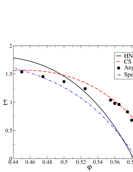
Figure 2.7: Equilibrium complexity $\Sigma(\varphi)$ as a function of the packing fraction. The full line is from the HNC equation of state (see Fig. 2.1), the dashed line is from the Carnahan–Starling equation of state. The black dots are from the numerical computation of Angelani et al. [57], the dot–dashed line is extrapolated from the numerical data reported by Speedy [54].

In Fig. 2.7 the equilibrium complexity $\Sigma(\varphi)$, obtained substituting the HNC and the CS expression for $S(\varphi)$ and $Y(\varphi)$ in Eq. (2.48), is reported. The results are compared with recent numerical results of Angelani et al. [57] obtained on a $50:50$ binary mixture of spheres (to avoid crystallization) with diameter ratio equal to $1.2$: the vibrational entropy was estimated using the procedure described in [49, 50] and the complexity was computed as $S(\varphi)-S_{vib}(\varphi)$. A quantitative comparison is difficult here because in the case of a mixture there can be corrections related to the mixing entropy, $S_{mix}\sim\log 2$. Nevertheless the data are in good agreement with our results. A detailed comparison would require the extension of the computation to binary mixtures following [49].

Another numerical estimate of $\Sigma(\varphi)$ was previously reported by Speedy [54], who rationalized his numerical data assuming a Gaussian distribution of states and a particular form for the vibrational entropy inside a state. The free parameters were then fitted from the liquid equation of state. The curve obtained by Speedy also agrees with our results.

Both the HNC and the CS estimates of the Kauzmann density ($\varphi_{K}=0.582$ and $\varphi_{K}=0.617$ respectively) fall, as it should be, between the Mode–Coupling dynamical transition that is $\varphi_{MCT}\sim 0.56$ [25, 26], and the Random Close Packing density that is estimated in the range $\varphi=0.64\div 0.67$, see e.g. [59].

A computation of $\Sigma(\varphi)$ based on very similar ideas was presented in [58], where a very similar estimate of $\varphi_{K}\sim 0.62$ was obtained. However in [58] the complexity was found to be $\Sigma\sim 0.01$, i.e. two orders of magnitude smaller than the one obtained from the numerical simulations. This negative result is probably due to some technical problem in the assumptions of [58].

2.6.2 Equation of state of the glass

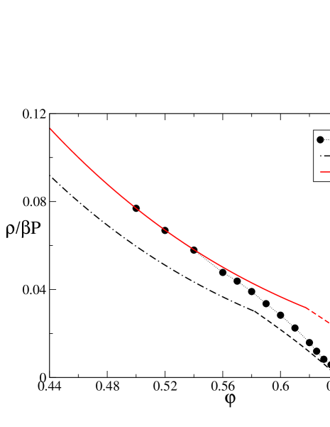
Figure 2.8: Inverse reduced pressure $\frac{\rho}{\beta P}$ of the Hard Sphere liquid as a function of $\varphi$. The black dots are from the simulation of Rintoul and Torquato [52]. The full line is obtained from the CS equation of state while the dot–dashed line is from the HNC equation of state. The dashed parts of the two curves correspond to the (ideal) glass phase. Note that all the curves are quasi–linear functions of $\varphi$ in the glass phase.

In Fig. 2.8 the numerical data for the pressure of the Hard Sphere liquid at high $\varphi$, obtained by Rintoul and Torquato [52], are reported. The data were obtained extrapolating at long times the relaxation of the pressure as a function of time after an increase of density starting from an equilibrated configuration at lower density. Also reported are the curves of the pressure as a function of the density obtained from the HNC and CS equations, both in the liquid and in the glass state.

The agreement of the HNC curve with the data is not very good even in the liquid phase, due to the modest accuracy of the HNC equation of state. However, its qualitative behavior is similar to the numerical data, and in particular the quasi–linear behavior of the inverse reduced pressure in the glass phase found in [52, 54], $\frac{\rho}{\beta P}\propto\varphi_{c}-\varphi$, is reproduced by the HNC curve. The HNC pressure of the glass diverges at $\varphi_{c}=0.640$ as discussed in section 2.4.1; the latter is the HNC estimate of the random close packing density.

The CS curve describes well the pressure in the liquid phase [68]. Comparing the curve with the data of Rintoul and Torquato, one notices that the glass transition happens in the numerical simulation at a density $\varphi_{g}\sim 0.56$ smaller than the one predicted by the CS curve, $\varphi_{K}=0.617$, and very close to the Mode–Coupling transition density, $\varphi_{MCT}\sim 0.56$. This is not surprising, since the relaxation time grows fast on approaching the ideal glass transition; at some point it becomes larger than the experimental time scale and the liquid falls out of equilibrium becoming a real glass. It is likely that the data of Ref. [52] describe the pressure of a real nonequilibrium glass, while the replica computation gives the pressure of the ideal equilibrium glass, that cannot be reached experimentally in finite time.

2.6.3 Random close packing

Both the HNC and CS equations predict the existence of a random close packing density $\varphi_{c}$ where the pressure and the value of the radial distribution function $\tilde{g}(r)$ in $r=D$ diverge. The HNC estimate is $\varphi_{c}=0.640$, in the range of the values ($\varphi_{c}=0.64\div 0.67$) reported in the literature. The CS estimate is $\varphi_{c}=0.683$ and it is also a value consistent with numerical simulations.

The reader should notice that the theoretical value for $\varphi_{c}$ is related to the ideal random close packing; however the states corresponding to this value of $\varphi_{c}$ can be reached by local algorithms, like most of the algorithms that were used in the literature, in a time that should diverge exponentially with the volume. Some caution should be taken in using the data obtained by numerical simulations. The question of which is the value of the density that can be obtained in large, but finite amount of time per particle is very interesting and more relevant from a practical point of view: however we plan to study it at a later time.

Note that the result for the mean coordination number $z$ of section 2.5, that gives $z=6$ at $\varphi=\varphi_{c}$ in $d=3$, is independent of the particular form chosen for $S(\varphi)$, and thus is valid for both the HNC and CS equations of state. The value $z=6$ has been reported in many studies [62, 63, 64, 65, 66].

2.6.4 Conclusions

The replica method of [15, 37] has been succesfully applied to the study of the ideal glass transition of Hard Spheres, and in general of potentials such that the pair distribution function $g(r)$ shows discontinuities, starting from the replicated HNC free energy and expanding it at first order in the cage radius $\sqrt{A}$.

This result allowed to compute from first principles the configurational entropy of the liquid as well as the thermodynamic properties of the glass up to the random close packing density. The computation is based on the HNC equation of state, that is known to yield a poor quantitative description of the liquid state at high density. Nevertheless, it is found that the qualitative scenario for the ideal glass transition that emerges from the replicated HNC free energy is very reasonable. In particular, a complexity $\Sigma\sim 1$, a Kauzmann density $\varphi_{K}=0.582$, and a random close packing density $\varphi_{c}=0.64$. All these results compare well with numerical simulations.

Using, on a phenomenological ground, the Carnahan–Starling equation of state instead of the HNC equation of state as input for the calculations, it was also possible to compare the results with the high–density pressure data of Rintoul and Torquato showing that they are indeed compatible with the observation of a real glass transition.

Moreover, it was found that the mean coordination number in the amorphous packed states is $z=2d$ irrespective of the equation of state used for the liquid, in very good agreement with the result of numerical simulations and with theoretical arguments [62, 63, 66, 65].

It is worth to note that these results do not prove the existence of a glass transition for the Hard Sphere liquid, as they derive from a particular approximation for the molecular liquid free energy (the HNC approximation), and, in general, other approximation such as the Percus–Yevick are possible [68].

Chapter 3 Correlation between fragility of the liquid and the vibrational properties of its glass

3.1 Introduction

The identification of the microscopic details that, in a given glass former, determine the temperature dependence of the viscosity, and thus the value of the fragility, is a long standing issue in the physics of supercooled liquids and glassy state. Large numerical and theoretical effort has been devoted to the attempt to relate the fragility to the specific interparticle interactions (e. g. strong glasses are often characterized by highly directional covalent bonds, while the fragile one have more or less isotropic interactions). The phenomenological relevance of the concept of fragility relies on the correlations that have been found between this index and other properties of glass-forming liquids. Examples of these correlations are the specific heat jump at $T_{g}$ (see Eq. (1.7) and [3]), the degree of stretching in the non-exponential decay of the correlation functions in the liquid close to $T_{g}$ [69], the visibility of the Boson peak at the glass transition temperature [70], or the temperature behavior of the shear elastic modulus in the supercooled liquid state [71]. Recently a strong correlation between fragility of the liquid and vibrational properties of its glass has been found [72].

3.1.1 Fragility and number of states

Recently, the attention has been focused on the possible relation existing between fragility and the properties of the (free) energy landscape, more specifically the (free) energy distribution of the minima and the properties of the basins of attraction of such minima. A key point is the validity of the Adam-Gibbs relation (1.6):

$$\tau(T)=\tau_{\infty}\exp\left(\frac{\cal E}{T\Sigma(T)}\right)\ .$$ (3.1)

By using the Adam-Gibbs relation, one could expect to relate fragility to the properties of $\Sigma(T)$, i.e., to the distribution of basins in the phase space of the system. For example, many authors proposed that fragile systems should have an higher number of states, i.e. a larger complexity, with respect to strong ones [1, 73, 74, 75].

However, this possibility is frustrated by the lack of knowledge on the parameter ${\cal E}$. Some theories attempting to compute ${\cal E}$, summarized in section 1.4.3, appeared only recently and in general the theory of the Adam–Gibbs relation is still at an early stage of development.

Unfortunately, even if a model for $\Sigma(T)$ is chosen, so the total number of states is fixed, one can obtain the whole range of experimentally observed fragilities by varying ${\cal E}$: fragility is related to $\Sigma(T)$ by Eq. (1.7), but the value of $T_{g}$ depends strongly on ${\cal E}$. More specifically, in [76] it was observed that for a large class of models for $\Sigma(T)$ - where $\Sigma(T)$ is a concave function of $T$ that vanishes at a given temperature $T_{K}$ and assumes its maximum $\Sigma_{\infty}$ at high temperature (“Gaussian-like models”) - the relevant parameter that actually determines the fragility is

$$D=\frac{\cal E}{T_{K}\Sigma_{\infty}}\ .$$ (3.2)

For example, if $\Sigma(T)=\Sigma_{\infty}\left(1-\frac{T_{K}}{T}\right)$ - the form that is commonly used to fit experimental data, see Eq. (1.5) and Fig. 1.2 - is substituted in Eq. (3.1) and the fragility is calculated from Eq. (1.2), one gets

$$\frac{m_{A}}{17}=17\log 10\,D^{-1}+1\ .$$ (3.3)

Thus, fragility appears to be determined by the ratio between ${\cal E}$ (measured in units of $k_{B}T_{K}$) and the total number of states $\Sigma_{\infty}/k_{B}$; it is related to both the distribution of minima (through $\Sigma_{\infty}$) and the characteristic of the transition path between them (through $\cal E$). The relation between fragility and phase space properties can be even more complicated, in those cases where the function $\Sigma(T)$ does not belong to the Gaussian class.

3.1.2 Fragility and vibrational properties of the glass

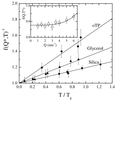
Figure 3.1: From [72]: (Left) The inverse nonergodicity factor $f(Q^{*},T)^{-1}$ for $Q^{*}=2\,{\rm nm}^{-1}$ and for three different substances as a function of $T/T_{g}$. In the inset, the wave vector dependence of $f(Q,T)$ is shown at fixed temperature $T^{*}$ to demonstrate that $f(Q^{*},T)\sim\lim_{Q\rightarrow 0}f(Q,T)$. (Right) Correlation plot of the fragility and the index $\alpha$ defined in Eq. (3.4).

Recently a strong correlation between fragility and the vibrational properties of the glass at low temperatures has been found [72]. The nonergodicity factor $f(k,T)$ defined in Eq. (1.8) was measured, by mean of inelastic X-rays scattering, in the (nonequilibrium) glass phase after a quench from high temperature. In Fig. 3.1 the temperature dependence of $f(k\sim 0,T)$ is shown. It is found that $f(k\sim 0,T)^{-1}$ is approximately linear in $T/T_{g}$ and an index $\alpha$ is defined as the slope of the curves in Fig. 3.1:

$$\alpha(T_{g})=\lim_{k\rightarrow 0}\left.\frac{d[f(k,T)]^{-1}}{d(T/T_{g})}\right|_{T=0}\ .$$ (3.4)

The index $\alpha$ has an explicit dependence on $T_{g}$ (as $\frac{d}{d(T/T_{g})}=T_{g}\frac{d}{dT}$). Moreover, it depends on $T_{g}$ also because depending on the value of $T_{g}$ (i.e. on the experimental time scale) different states are selected: in particular, the states that are selected are the equilibrium states at $T=T_{g}$, as exactly at this value of temperature the system falls out of equilibrium. The order parameter $f(k,T)$ of a given state is a measure of the volume of this state in the phase space, and can in principle depend on the state in which the sistem is frozen below $T_{g}$. In particular, in [72] an expression of $\alpha$ in terms of the harmonic vibrational properties of the states (eigenmodes of the disordered structure), was derived: and the eigenmodes will depend on the particular structure in which the system is frozen, that is, on the equilibrium structure at $T=T_{g}$.

In the right panel of Fig. 3.1 it is shown that the index $\alpha$ is strongly correlated with the fragility index $m_{A}$. This finding implies the existence of a relation between three features of the energy landscape: the energy of the minima, the transition paths between them (that together determine the fragility) and the Hessian matrix, evaluated at the minima themselves, that fixes the vibrational properties.

3.2 Fragility in mean field $p$-spin models

As discussed in the first chapter, mean field models such as the disordered $p$-spin model provide an useful framework to understanding many aspects of the glass transition. Using the arguments of sections 1.4.1 and 1.4.3 one can relate the quantities appearing in the Adam–Gibbs relation, i.e. $\Sigma(T)$ and ${\cal E}(T)$, to the mean field potential $V(q,T)$ that is expected to describe short range models at the local level. One can then investigate the $p$-spin models as solvable models of “glass”, where the distribution of minima is “Gaussian-like” as in real structural glasses, and both the vibrational properties of the minima and the energy barrier ${\cal E}(T)$ can be analytically estimated. The $p$-spin models are “Gaussian-like”, in the sense that their complexity - even if the distribution of states is not exactly Gaussian - is known to be a concave function of the temperature, that vanishes at $T_{K}$ and assumes its maximum at $T_{d}$, without any inflection point in between, see [22] and Fig. 1.5, yielding a form very similar to Eq. (1.5) for $\Sigma(T)$.

In this chapter, both the spherical and Ising version of the $p$-spin model will be investigated, in order to check whether one can reproduce the correlation between fragility of the liquid and the vibrational properties of its glass found in [72] by studying the geometry of the phase space of these models. Moreover the question of the existence of a correlation between fragility and number of states [73, 74, 75] will be addressed.

The mean field models will be considered as models for the local properties of a short range glass, as indicated by the arguments discussed in sections 1.4.1 and 1.4.3. Then, the existence of the dynamical transition will be ignored, being an artifact of mean field, and it will be assumed that it is possible to equilibrate the system below $T_{d}$ with a relaxation time following the Adam–Gibbs relation (3.1) with ${\cal E}$ and $\Sigma$ determined by the mean field potential $V(q,T)$. As will be clarified below, the fragility of the models can be varied by varying the parameter $p$.

3.2.1 Definition of the relevant observables

It is useful to summarize the definition of all the quantities that will be computed, that are listed below:

$$\begin{array}[]{ll}T_{K}&\text{Thermodynamical transition temperature}\\ T_{g}&\text{Glass transition temperature}\\ T_{d}&\text{Dynamical transition temperature}\\ \Sigma(T_{g})&\text{Complexity at $T_{g}$}\\ m(T_{g})&\text{Fragility}\\ \alpha(T_{g})&\text{``Volume'' of the equilibrium states at $T_{g}$}\\ {\cal E}(T_{g})&\text{``Barrier height'' at $T_{g}$}\end{array}$$

Setting $k_{B}=1$, all the above quantities are either dimensionless or have the dimension of an energy; in the $p$-spin model -as usual in classical spin models- a natural energy scale $J$ appears as the strenght of the couplings between spins. Thus, if one additionally sets $J=1$, all the quantities become dimensionless.

Temperatures

From the two replica potential $V(q,T)$ discussed in section 1.3.2 the complexity $T\Sigma(T)=V(q_{min}(T),T)-V(0,T)$ and the barrier height ${\cal E}(T)=V(q_{max}(T),T)-V(q_{min}(T),T)$ are extracted as functions of the temperature. Then, the thermodynamical transition temperature $T_{K}$ is defined as the temperature where the complexity vanishes: $\Sigma(T_{K})=0$, and the value of $V$ at the secondary minimum becomes equal to zero (see Fig. 1.6). The dynamical transition temperature $T_{d}$ is the temperature at which the metastable minimum first appears, so it is defined by ${\cal E}(T)=0$.

Then, an Adam–Gibbs like relation in which ${\cal E}(T)$ plays the role of the energy barrier and $T\Sigma(T)$ of the configurational entropy is considered. Starting from the Adam–Gibbs relation (3.1) one defines $T_{g}$ by $\tau(T_{g})/\tau_{\infty}=$ const, or, equivalently, by

$$\frac{{\cal E}(T_{g})}{T_{g}\Sigma(T_{g})}={\cal C}\ .$$ (3.5)

The value of the constant ${\cal C}$ determines the value of $T_{g}$. It is arbitrary because proportionality factors have always been neglected, so it will be fixed in order to obtain reasonable values for the fragility, $m_{A}/17\sim 1\div 10$, as observed in experiments, see Fig. 3.1. It will turn out that the analysis is not strictly dependent on the value of $T_{g}$ (and of ${\cal C}$), the behavior of the various quantities at $T_{g}$ being representative, as will be shown, of a general trend observed at all temperatures $T\in[T_{K},T_{d}]$ by varying $p$. Different choices of the constant ${\cal C}$ change only quantitatively the results, while the qualitative picture stays the same.

Complexity, barrier heights and fragility

Given a definition of $T_{g}$, the complexity at $T_{g}$ is simply $\Sigma(T_{g})$ and the barrier height ${\cal E}(T_{g})$: clearly, these two quantities are related by Eq. (3.5). Knowing the complexity as a function of the temperature, the fragility can be defined as in Eq. (1.7). To simplify the notations, the factor $17$ entering Eq. (1.7) will be neglected in the following and the fragility defined as:

$$m(T_{g})=1+T_{g}\frac{\Sigma^{\prime}(T_{g})}{\Sigma(T_{g})}\ .$$ (3.6)

The latter definition is very useful in a mean field context as - once a definition of $T_{g}$ has been chosen - it involves only the complexity, that is a well-defined quantity in mean field models. It is equivalent to the usual Angell definition of fragility if $\eta_{\infty}$ does not depend strongly on the material, and the Adam-Gibbs relation is assumed to be valid [76]. This definition of fragility has been shown to be correlated to the fragility defined from the relaxation time using experimental data in [3].

Volume of the states

The index $\alpha$ defined in [72] can be replaced by other equivalent - equivalent meaning positively correlated - definitions. An useful equivalent definition of $\alpha$ is

$$\alpha(T_{g})=\lim_{k\rightarrow 0}\Big{[}1-f(k,T_{g})\Big{]}\ .$$ (3.7)

As one can easily check observing Fig. 3.1, this definition is equivalent to Eq. 3.4 if the curves of $f(k,T)$ as function of $T$ for different materials do not intersect.

The quantity $f(k,T)$ (in the low-$k$ limit) can be identified in spin models with the self-overlap of the states as discussed in section 1.1.6. Thus, one can define

$$\alpha(T_{g})=1-q(T_{g})\ ,$$ (3.8)

where $q(T_{g})$ is the self-overlap of the equilibrium states at $T_{g}$, i.e., the value of $q$ where $V(q,T)$ has the secondary minimum at $T=T_{g}$ (see Fig. 1.6).

As the self-overlap of the states is related to their volume in phase space (high overlap corresponding to small states), a small value of $\alpha$ corresponds to small-volume states, while a big value of $\alpha$ corresponds to large-volume states. In this sense, $\alpha(T_{g})$ will be called “volume of the equilibrium states at $T_{g}$”. Note that a similar identification has been discussed in [72]: indeed, from Eq. (7) of [72] one can see that $\alpha$ is related to the curvatures of the minima of the potential (in the harmonic approximation), and that small curvatures (large volume) correspond to large $\alpha$, while high curvatures (small volume) correspond to small $\alpha$. This is consistent with the equivalence of the definition of $\alpha$ given in [72] and the one adopted here.

Summary of the definitions

To conclude this section, it is useful to give a short summary of all the definition discussed above. Calling $q_{min}(T)$ the value of $q$ where $V(q,T)$ has the secondary minimum, and $q_{max}(T)$ the value of $q$ where $V(q,T)$ has a maximum, the definitions are:

$$\begin{array}[]{lcl}\Sigma(T)&=&\big{[}V(q_{min}(T),T)-V(0,T)\big{]}/T\\ {\cal E}(T)&=&V(q_{max}(T),T)-V(q_{min}(T),T)\\ T_{K}&:&\Sigma(T_{K})=0\\ T_{g}&:&\frac{{\cal E}(T_{g})}{T_{g}\Sigma(T_{g})}={\cal C}\\ T_{d}&:&{\cal E}(T_{d})=0\\ m(T_{g})&=&1+T_{g}\frac{\Sigma^{\prime}(T_{g})}{\Sigma(T_{g})}\\ \alpha(T_{g})&=&1-q_{min}(T_{g})\\ \end{array}$$

The constant ${\cal C}$ has to be chosen in order for the fragility to be in the experimentally observed range, $m\sim 1\div 10$.

3.2.2 Spherical $p$-spin model

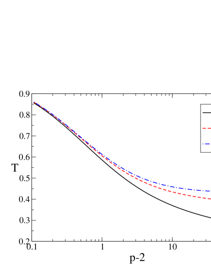
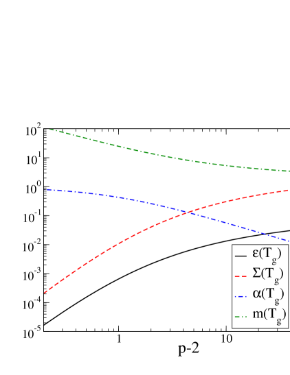
Figure 3.2: (Left) Thermodynamic transition temperature $T_{K}$, glass transition temperature $T_{g}$ and dynamical transition temperature $T_{d}$, and (right) fragility $m(T_{g})$, configurational entropy $\Sigma(T_{g})$, “volume” of the equilibrium states $\alpha(T_{g})$ and barrier height ${\cal E}(T_{g})$ for the $p$-spin spherical model as a function of $p-2$.

The full expression for $V(q,T)$ in the $p$-spin spherical model has been computed in [36, 39]. However, a simplified expression can be used when the value of $V(q,T)$ on its stationary points is considered:

$$V(q,T)-F(T)=-\frac{\beta}{4}q^{p}-\frac{T}{2}\log(1-q)-\frac{Tq}{2}\ .$$ (3.9)

This function has been shown in section 1.3.3 to coincide with the correct $V(q,T)$ on each stationary point of $V(q,T)$. If one is interested only in the value of $V(q,T)$ on its stationary points, the use of the correct $V(q,T)$ calculated in [36, 39] or of the one given by Eq. (3.9) gives exactly the same result.

Note that, while the model is defined only for integer $p$, Eq. (3.9) makes sense also for real $p$; therefore the behavior of the different quantities for any real $p\geq 2$ can be investigated. In particular, the $p\rightarrow 2$ limit is interesting being related to a diverging fragility ($T_{d}\rightarrow T_{K}$) and to the discontinuous 1rsb transition becoming a continuous one.

Temperatures

From Eq. (3.9) one can compute the three temperatures $T_{K}$, $T_{g}$ and $T_{d}$ as functions of $p$. Their behavior is reported in Fig. 3.2. For $p\sim 2$, the difference between $T_{K}$ and $T_{g}$ is very small, therefore the system is very fragile; for $p\rightarrow\infty$ the Kauzmann temperature approaches zero (as $1/\sqrt{\log p}$), while the glass transition temperature remains finite. The system therefore becomes stronger and stronger on increasing $p$.

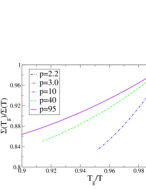
Figure 3.3: Scaled plot of the complexity, $\Sigma(T_{g})/\Sigma(T)$, as a function of $T_{g}/T$ for the $p$-spin spherical model at different values of $p$. The figure has to be compared with Fig. 1.3; in both figures fragility is the slope of the curves in $T_{g}/T=1$. The system becomes stronger on increasing $p$.

Complexity and fragility

The same observation can be made more quantitative by considering an “Angell plot” for the complexity [3]: in Fig. 3.3 the complexity $\Sigma(T)$ is plotted as a function of the temperature, for different values of $p$. The choice of the particular scaling that appears in Fig. 3.3 has been made in order to make a close correspondence with Fig. 1.3, extracted from [3]. The curves for different values of $p$ are ordered from bottom to top. The same behavior is observed in glass formers of different fragility. Indeed, the index of fragility defined in Eq. (3.6) is exactly one plus the slope in $T_{g}/T=1$ of the curves in Fig. 3.3:

$$m(T_{g})=1+T_{g}\frac{\Sigma^{\prime}(T_{g})}{\Sigma(T_{g})}=1+\left.\frac{d[\Sigma(T_{g})/\Sigma(T)]}{d[T_{g}/T]}\right|_{T=T_{g}}\ .$$ (3.10)

The fragility index $m$ is shown in Fig. 3.2 as a function of $p$. It is a decreasing function of $p$. Its values are in the range observed for experimental system due to the (arbitrary) choice of the constant ${\cal C}$ appearing in Eq. (3.5), ${\cal C}=0.1$. In Fig. 3.2 $\Sigma(T_{g})$ is also reported as a function of $p$. It is an increasing function of $p$, that diverges as $\log p$ for $p\rightarrow\infty$: thus, the number of states in this system is a decreasing function of the fragility.

Barrier heights and volume of the states

In Fig. 3.2 the barrier height ${\cal E}(T_{g})$ is also reported as a function of $p$, together with the index $\alpha(T_{g})=1-q(T_{g})$ that was called “volume” of the equilibrium states at $T_{g}$. In this model the states become smaller on increasing $p$, while the barriers separating them increase. The correlations between these quantities will be discussed in section 3.3, where a geometric description of the evolution of the phase space of this model at different $p$ will be proposed, that relates fragility to geometric properties of the phase space.

3.2.3 Ising $p$-spin model

The Ising $p$-spin model is another popular model for the study of the glass transition [10, 17, 77]. Its Hamiltonian is given by Eq. (1.10), where the variables $\sigma_{i}$ are Ising spins, $\sigma_{i}=\pm 1$, and the spherical constraint is absent. For the Ising $p$-spin model, the two-replica potential $V(q,T)$ is given by

$$V(q,T)-F(T)=\beta\frac{p-1}{4}q^{p}+\beta\frac{p}{4}q^{p-1}-\frac{\int{\cal D}z\cosh(\Lambda z)\log\cosh(\Lambda z)}{\int{\cal D}z\cosh(\Lambda z)}\ ,$$ (3.11)

where ${\cal D}z=\exp(-z^{2}/2)\ dz$, and $\Lambda^{2}=\beta^{2}\frac{p}{2}q^{p-1}$.

Note that the total number of states in the Ising $p$-spin model cannot be greater than $2^{N}$ (the total number of configurations), and hence $\Sigma(T)\leq\log 2$, while in the spherical model $\Sigma(T_{g})$ diverges as $\log p$ for $p\rightarrow\infty$, as previously discussed.

Temperatures

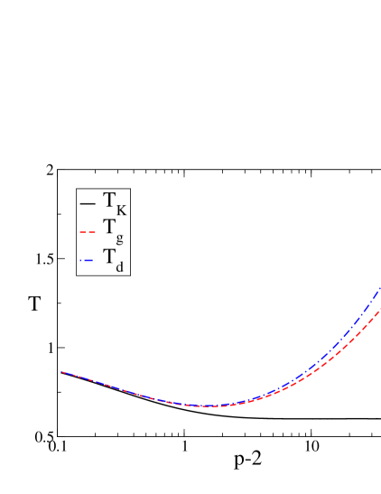
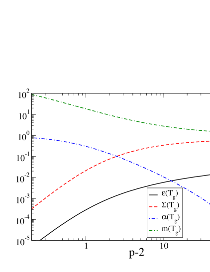
Figure 3.4: (Left) Thermodynamic transition temperature $T_{K}$, glass transition temperature $T_{g}$ and dynamical transition temperature $T_{d}$ and (right) fragility $m(T_{g})$, configurational entropy $\Sigma(T_{g})$, “volume” of the equilibrium states $\alpha(T_{g})$ and barrier height ${\cal E}(T_{g})$ for the $p$-spin Ising model as a function of $p-2$.

The first consequence of this difference is observed when studying the transition temperatures as functions of $p$ (see Fig. 3.4). Indeed, as in the spherical model, $T_{K}\sim T_{g}$ for $p\sim 2$, and $T_{g}\gg T_{K}$ for $p\rightarrow\infty$. But, in this model, $T_{K}$ tends to a finite value at large $p$, while $T_{g}$ and $T_{d}$ diverge. This behavior can be understood recalling that for a “Gaussian-like” model one has $T_{K}\sim 1/\sqrt{\Sigma_{\infty}}$, $\Sigma_{\infty}$ being the total number of states, i.e. the maximum of $\Sigma(T)$ [76].

Complexity and geometric properties of the phase space

The “Angell plot” for the complexity of the Ising $p$-spin model looks very similar to the one of the spherical model, Fig. 3.3, so it is not useful to report it.

Having fixed an appropriate value for the constant ${\cal C}$ in Eq. (3.5) (${\cal C}=0.02$, different from the value chosen in the spherical case), the behavior of the fragility as a function of $p$ is also very similar to the one of the spherical model. The same behavior is found for the other quantities under study, as one can deduce from a comparison of Fig. 3.4 and Fig. 3.2, the main difference being the discussed behavior of $\Sigma(T_{g})$ at large $p$.

Vibrational properties and volume of the states

Another relevant difference between the spherical and the Ising model is that, in the latter, harmonic vibrations are not present (the variables being discrete): we have $q(T)\rightarrow 1$ exponentially for $T\sim 0$, and the definition of $\alpha$ via Eq. (3.4) gives $\alpha=0$ for all $p$. However, the definition given in Eq. (3.8) and used in these calculations gives a reasonable result also in absence of harmonic vibrations.

3.3 Correlations between different properties of the phase space

In this section the correlations between the quantities under study will be investigated, trying to relate fragility to the phase space geometry. The results will be compared with the general consideration of [76], and with the experimental results of [72].

3.3.1 Fragility and volume of the states

In [72] it has been established that fragility is positively correlated with the index $\alpha$ defined in section 3.2.1. In other words, fragile systems have large basins while strong systems have small basins. In Fig. 3.5 the fragility $m$ is plotted as a function of $\alpha$ parametrically in $p$ for the investigated systems. The curve $m(\alpha)$ is very similar for the two models - remember that the only adjustable parameter is the constant ${\cal C}$ in Eq. (3.5). By comparison with Fig. 3.1, one can conclude that the model has a behavior similar to the one of real systems. Surprisingly, also the linear correlation between $m$ and $\alpha$ is reproduced for $\alpha\leq 0.4$. Thus, mean field $p$-spin models are able to describe the relation between fragility and the volume of the basins visited around $T_{g}$ found in [72].

3.3.2 Fragility, barrier heights and number of states

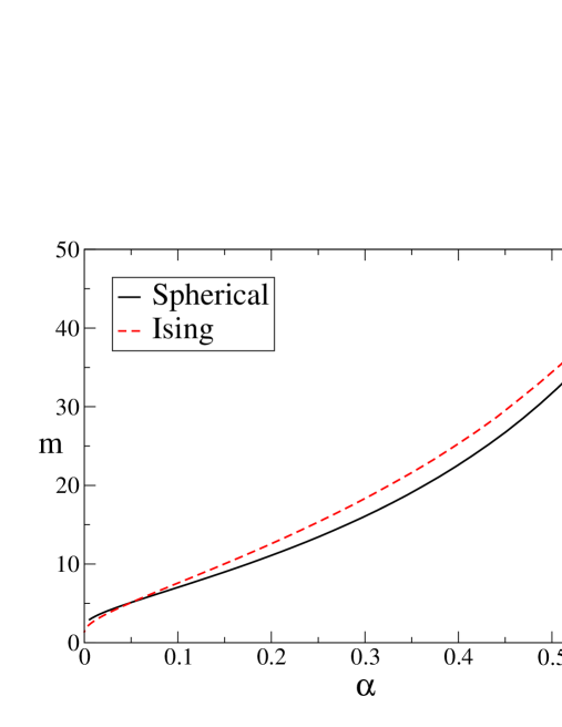
Figure 3.5: Fragility versus $\alpha$ for the spherical and Ising $p$-spin models. The curve is very similar for the two models, and is consistent with the correlation found in [72], see Fig. 3.1. The linear correlation is reproduced for $\alpha\leq 0.4$.

It has been conjectured that fragile systems have a larger number of states than strong ones, even if the total number of states is not an experimentally accessible quantity and numerical simulations give contradictory results [73, 74, 75]. However, in the models considered here the behavior is exactly the opposite. In Fig. 3.6 $\Sigma(T_{g})$ is reported as a function of the fragility: the total number of states is a decreasing function of the fragility.

This point was discussed in detail in [76], where the possibility of correlating fragility with the total number of states for general models of $\Sigma(T)$ was discussed, assuming the validity of the Adam-Gibbs relation, Eq. (3.1). The conclusion was that the knowledge of the distribution of states is not enough to determine the fragility. Indeed, the relevant parameter, for a general “Gaussian-like” distribution of states, is

$$D=\frac{{\cal E}(T_{g})}{T_{K}\Sigma(T_{g})}\ .$$ (3.12)

Note that in Eq. (3.12) ${\cal E}$ has to be evaluated at $T=T_{g}$ because in the considered models the barrier height ${\cal E}$ is a $T$-dependent quantity, while in the Adam-Gibbs relation it is usually assumed to be a constant. However, the Adam-Gibbs relation has been tested around $T_{g}$, therefore, to a good approximation, one can fix ${\cal E}$ to be a constant equal to its $T=T_{g}$ value. The parameter $D$ is inversely proportional to the fragility $m$: therefore $m\sim\Sigma/{\cal E}$, and fragility turns out not to be simply correlated to the total number of states. If the “barrier heights” grow faster than the total number of states, fragility can be a decreasing function of $\Sigma$: this is indeed the case in the considered models.

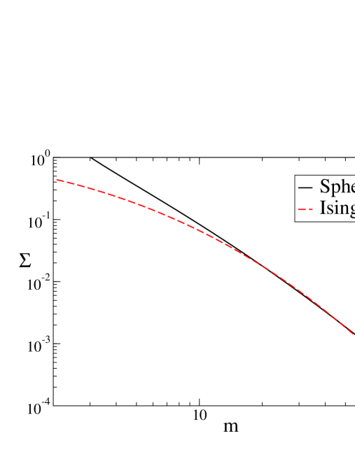
Figure 3.6: Total number of states (represented by the complexity at $T_{g}$) as a function of the fragility $m$ for the $p$-spin models.

Indeed, from Fig. 3.2 and Fig. 3.4, one observes that the barrier height is an increasing function of $p$. Using Eq. (3.5), Eq. (3.12) can be written as

$$D={\cal C}\frac{T_{g}}{T_{K}}\ .$$ (3.13)

Therefore, from Fig. 3.2 and Fig. 3.4, $D$ is an increasing function of $p$ that diverges for $p\rightarrow\infty$, as the ratio $T_{g}/T_{K}$ increase on increasing $p$ for both models. Thus, in the considered models the height of the barriers (in units of $T_{K}$) increases faster than the total number of states. This explains why one observes an inverse correlation between fragility and the total number of states, as discussed above and in [76].

3.3.3 A geometric picture of the phase space

Figure 3.7: Sketch of the evolution with $p$ of the $p$-spin free energy landscape: at small $p$ there is a small number of states of large volume separated by low barriers; at high $p$ there is a large number of states of small volume separated by high barriers. The height of the barriers increase faster than the number of states: thus, fragility is a decreasing function of $p$.

The information obtained in the previous sections can be collected in a geometric picture of the evolution with $p$ of the $p$-spin model free energy landscape. Indeed, on increasing $p$:
i) The total number of states increases.
ii) The volume of the states decreases ($\alpha$ decreases).
iii) The height of the barriers between states increases.
Thus, we get the picture of a landscape where, on increasing $p$, a great number of small states with very high curvatures and separated by very high barriers appear: a sketch of this evolution is given in Fig. 3.7. The behavior of the fragility in this situation is related to the behavior of $\Sigma/{\cal E}$, the ratio between number of states and height of the barriers between them: in these models, it turns out that ${\cal E}$ increase faster than $\Sigma$, and the fragility is a decreasing function of $p$.

This behavior is consistent with the fact that fragility turns out to be positively correlated with the “volume” of the states as measured by $\alpha$. Indeed, if, on the contrary, the barrier height grew slower than the total number of states (equivalently, if $m$ would be positively correlated with the total number of states), there should be also an inverse correlation between $m$ and $\alpha$, in disagreement with what is experimentally observed.

In the $p\rightarrow 2$ limit, where the fragility becomes infinite, the second derivative with respect to $q$ of the potential $V(q,T)$ calculated in $q=0$ and $T=T_{K}=T_{d}$ vanishes (see Fig. 1.6) and the so-called spin glass susceptibility diverges at the critical temperature. In other words when the fragility becomes infinite soft modes appear at the critical temperature supporting the previously presented physical picture.

Note that the outlined picture is valid for “Gaussian-like” models, i.e., models where the complexity is a concave function of the temperature that vanishes at $T_{K}$ without any inflection point. These models seem to describe correctly the distribution of basins in real systems only for relatively high fragilities. The behavior of the complexity (or configurational entropy, or excess entropy) as a function of temperature for very strong systems is still an open problem, see e.g.  [78, 79]; our discussion may not apply to these systems.

The main prediction of this analysis is that the total number of states $\Sigma_{\infty}$ and the Adam-Gibbs barrier ${\cal E}$ should both be decreasing functions of the fragility. This prediction disagrees with the statement of [73, 74, 75] that fragile systems should have an higher number of states with respect to strong ones. A critical analysis of this works can be found in [76]. Unfortunately, existing data are not sufficient to strictly test this prediction; the excess entropy is available only for few experimental systems, and numerical simulations are performed in a temperature range where the fragility of the investigated systems is approximately the same. Hopefully this predictions will be tested in the future.

Part II Nonequilibrium

Chapter 4 Nonequilibrium stationary states and the fluctuation theorem

4.1 Introduction

4.1.1 A critical review of the ergodic hypothesis

The statistical mechanics of equilibrium states can be constructed starting from the ergodic hypothesis of Boltzmann, see e.g.  [30] for a modern review. An equilibrium system is, for instance, a system of $N$ classical particles enclosed in a volume $V$ which interact between themselves and with the wall of the container only by conservative forces. The phase space of the system can be divided in suitable cells $\Delta$, such that the dynamics can be represented as a discrete-time map $S\Delta=\Delta^{\prime}$ acting on the cells. Then, the ergodic hypothesis is the assumption that $S$ is a one-cycle permutation of the cells with constant energy (because the energy is kept constant by the time evolution). This means that all the cells are visited sequentially: and if one considers an observable $F(\Delta)$, the time average

$$\left\langle F\right\rangle=\lim_{\tau\rightarrow\infty}\frac{1}{\tau}\sum_{t=0}^{\tau-1}F(S^{t}\Delta)\ ,$$ (4.1)

starting from any initial condition $\Delta$ such that $U(\Delta)=U$, does not depend on the initial condition and is simply given by the flat average over the cells with energy $U$,

$$\left\langle F\right\rangle=\frac{1}{{\cal N}(U,V)}\sum_{\Delta:U(\Delta)=U}F(\Delta)\ ,$$ (4.2)

where ${\cal N}(U,V)$ is the total number of such cells. Starting from the ergodic hypothesis Boltzmann was able to prove that, if one defines the observables $T$ (temperature), $U$ (internal energy), and $P$ (pressure) in terms of the average kinetic energy, potential energy, and momentum transfer to the container walls respectively, a function $S(U,V)$ (entropy) exists such that

$$dS=\frac{dU+PdV}{T}\ .$$ (4.3)

The function $S(U,V)$, in the construction of Boltzmann, is $S(U,V)=k_{B}\log{\cal N}(U,V)$. The ergodic hypothesis says that the statistical measure describing the equilibrium macroscopic state on the phase space of the system is simply the flat measure on the surface of constant total energy $U$. The ensemble of these measures, obtained by varying the values of the external parameters $U$, $V$, is called the microcanonical ensemble. Then one can show that different ensembles of measures can be defined, and that they are equivalent, in the sense that they give rise to the same macroscopic relations between observables and in particular that Eq. (4.3) holds for all of them.

Despite this success, the ergodic hypothesis was criticized, because it seemed impossible to derive the irreversible laws of thermodynamics from the microscopic reversible equations of motion. Indeed, if the dynamics $S$ is a one-cycle permutation of the cells, after a given recurrence time the system must come back to the cell in which it was prepared at the initial time. The observation of Boltzmann was that this recurrence time, for a macroscopic system of $N\sim 10^{23}$ particles, could be estimated to be essentially infinite on any reasonable time scale, so that reversibility could not be observed for macroscopic systems.

However, this argument seems to make the ergodic hypothesis meaningless: if the time needed for the system to visit all the cells is much larger than any experimentally accessible time scale, the replacement of the average over the time evolution with the flat average over the cells is unjustified. Boltzmann realized this difficulty [30] and solved it observing that, for a macroscopic system, the thermodynamically interesting observables are essentially constant on phase space, thanks to the law of large numbers. Then, even if the system visits only a small portion of its phase space on the experimental time scale, the replacement of the time average with a flat average on phase space gives the correct result.

Thus, the ergodic hypothesis alone is not a justification of the thermodynamics. However it correctly suggests that the averages of the interesting observables can be computed using the flat measure on phase space, provided that the size of the system is large. It is even not important to prove that a given physical system is ergodic, and it is likely that many of the models which are commonly used to describe physical systems are not ergodic. The ergodic hypothesis is relevant because it allows to identify the correct measure describing the macroscopic equilibrium states on the microscopic scale.

4.1.2 Nonequilibrium states and the chaotic hypothesis

One could ask if a similar construction can be repeated in the case of a stationary nonequilibrium system. For instance one can think to a system of $N$ interacting particles in $d$ dimensions, enclosed in a container of volume $V$, subjected to nonconservative forces and kept in a stationary state by a reversible mechanical thermostat. It will be defined by a differential equation $\dot{x}=X_{E}(x)$ where $x=(\dot{{\underline{q}}},{\underline{q}})\in R^{2dN}\equiv M$ (phase space) and

$$m\ddot{{\underline{q}}}={\underline{f}}({\underline{q}})+{\underline{g}}_{E}({\underline{q}})-{\underline{\theta}}_{E}(\dot{{\underline{q}}},{\underline{q}})$$ (4.4)

where $m$ is the mass of the particles, ${\underline{f}}({\underline{q}})$ describes the internal (conservative) forces between the particles (and between the particles and the walls of the container) and ${\underline{g}}_{E}({\underline{q}})$ represents the nonconservative “external” force acting on the system, which is assumed to depend smoothly on a parameter $E$ (e.g. the amplitude of the electric field). Finally, ${\underline{\theta}}_{E}(\dot{{\underline{q}}},{\underline{q}})$ is a mechanical force that prevents the system from acquiring energy indefinitely: this is why it is called a mechanical thermostat. Systems belonging to this class are frequently used as microscopic models to describe nonequilibrium stationary states induced by the application of a driving force (temperature or velocity gradients, electric fields, etc.) on a fluid system in contact with a thermal bath [80, 81]. The problem of which is the measure describing the stationary states of such a system is still matter of debate, but important progress have been achieved in recent times. They will be discussed in the rest of this chapter.

A first difficulty one has to face is that, for nonequilibrium stationary states, a well-established macroscopic theory similar to equilibrium thermodynamics does not exist [82]. From a microscopic point of view, the main difficulty is that the equation of motion (4.4) yields a phase space contraction rate

$$\sigma(x)=-{\rm div}X_{E}(x)\ ,$$ (4.5)

such that $\frac{d}{dt}dx=-\sigma(x)dx$, which has positive average [83], i.e. if $S_{t}x$ is the solution of Eq. (4.4) with initial datum $x$, for almost all $x$ w.r.t. the volume $dx$, one has

$$\sigma_{+}\equiv\left\langle\sigma(x)\right\rangle=\lim_{\tau\rightarrow\infty}\frac{1}{\tau}\int_{0}^{\tau}dt\,\sigma(S_{t}x)>0\ .$$ (4.6)

This means that phase space volume is not conserved by the time evolution, so the invariant measure cannot be the flat measure on phase space, and cannot even admit a density, i.e. be of the form $\mu(dx)=\mu(x)dx$: it will be concentrated on a set of zero volume in phase space. Also, this means that the description of the system in terms of cells $\Delta$ and the hypothesis that the dynamics is a simple one-cycle permutation cannot hold for nonequilibrium systems. Still a description in term of cells is possible but it does not lead to a satisfactory notion of “entropy” [84].

A very important step towards the construction of a statistical mechanics of nonequilibrium stationary states was the explicit construction of the invariant measure for a class of smooth chaotic dynamical systems, called Anosov systems [30, 85, 86, 87, 88, 89, 90, 91]. For these systems it was proved that almost all points w.r.t. the volume measure evolve so that all smooth observables have a well defined average equal to the integral over the invariant measure, i.e. for all smooth $F(x)$

$$\left\langle F(x)\right\rangle\equiv\lim_{\tau\rightarrow\infty}\frac{1}{\tau}\int_{0}^{\tau}dt\,F(S_{t}x)=\int\mu_{+}(dx)F(x)\ .$$ (4.7)

The measure $\mu_{+}(dx)$ is called Sinai–Ruelle–Bowen (SRB) distribution. In particular this holds for the phase space contraction rate $\sigma(x)$ and the relation $\sigma_{+}\geq 0$, see Eq. (4.6), was proved for these systems [83].

Anosov systems are paradigms of chaotic systems: and even if essentially none of the physically interesting systems could be proved to be Anosov, a chaotic hypothesis was proposed [92, 93], which states that nevertheless one can assume that chaotic motions (in the sense of motions with at least one positive Lyapunov exponent) exhibit some average properties of truly Anosov systems. In particular, it should be possible to compute the averages of the physically interesting observables using the SRB distribution.

This hypothesis is a natural generalization of the ergodic hypothesis, as the SRB distribution reduces to the flat distribution in the equilibrium case where $\sigma_{+}=0$. Similarly to the ergodic hypothesis, the chaotic hypothesis simply suggests that the invariant measure is the SRB measure, even if the system is not an Anosov system. But this allows to make some predictions on the macroscopic properties of systems like the one described by Eq. (4.4), similarly to what has been done by Boltzmann by proving that the ergodic hypothesis implies the validity of Eq. (4.3).

4.1.3 The fluctuation theorem

An interesting prediction of the chaotic hypothesis is the validity of a relation that concerns the large deviations of the phase space contraction rate, and that has been named fluctuation relation. The validity of this relation for a reversible Anosov map $S$ was proved (fluctuation theorem) in [92, 93]. Reversibility means that there is a metric–preserving map $I$ on the phase space $M$ such that $IS=S^{-1}I$ and is a key hypothesis for the validity of the fluctuation relation. For a map $S$ the phase space contraction rate is defined as

$$\sigma(x)=-\log|\det\partial S(x)|\ ,$$ (4.8)

and it is a smooth function on $M$. As discussed above the average of $\sigma(x)$ exists and is $\sigma_{+}\geq 0$. If $\sigma_{+}>0$, let:

$$p(x)=\frac{1}{\tau\sigma_{+}}\sum_{t=0}^{\tau-1}\sigma(S^{t}x)\ .$$ (4.9)

The function $p(x)$ has average $\langle\;p\;\rangle=1$ and distribution $\pi_{\tau}(dp)$ such that

$$\pi_{\tau}(\{p\in\Delta\})=e^{\tau\max_{p\in\Delta}\zeta_{\infty}(p)+o(\tau)}\;,$$ (4.10)

where the correction at the exponent is $o(\tau)$ w.r.t. $\tau$ as $\tau\rightarrow\infty$, and the function $\zeta_{\infty}(p)$ is analytic and convex in $p$. The fluctuation relation then reads:

$$\zeta_{\infty}(p)=\zeta_{\infty}(-p)+p\sigma_{+}\qquad{\rm for\ all}\ |p|<p^{*}\ ,$$ (4.11)

where $\infty>p^{*}\geq 1$ is a suitable (model dependent) constant that, in general, is different from the maximum over $\tau$ and $x$ of $p(x)$, and is defined by $\zeta_{\infty}(p)=-\infty$ for $|p|>p^{*}$.

The interesting fact is that the fluctuation relation has no free parameters: thus the simplest and more stringent check of the applicability of the chaotic hypothesis is a check of the fluctuation relation. Of course even if the check has a positive result this will not “prove” the hypothesis but it will at least add confidence to it. This test has been performed in a number of cases with positive result, by mean of numerical simulations [94, 95, 96, 97, 98, 99, 100, 101, 102] and experiments [103, 104, 105, 106].

In the following, after a brief review of the procedure that allows to construct the SRB measure for Anosov systems, the physical implications of the chaotic hypothesis will be discussed.

4.2 Sinai–Ruelle–Bowen (SRB) measures

4.2.1 Anosov systems

Anosov systems are paradigms of chaotic systems. They are defined as follows [91]. Given a compact, smooth and boundaryless manifold $M$ (phase space), a map $S\in C^{2}(M)$ is an Anosov map if:

(1) For all $x\in M$ the tangent plane to $M$ in $x$, $T_{x}$, admits a decomposition $T_{x}=T^{s}_{x}\oplus T^{u}_{x}$, such that

(2) the planes $T^{s,u}_{x}$ vary continuously w.r.t. $x$, i.e. the vectors defining them are continuous functions of $x$;

(3) the angle between $T^{s}_{x}$ and $T^{u}_{x}$, defined as the minimum angle between a vector in $T^{s}_{x}$ and a vector in $T^{u}_{x}$, is not vanishing;

(4) defining $\partial S$ the linearization matrix of $S$ in $x$, i.e. $S(x+\epsilon v)=S(x)+\epsilon\ \partial S(x)\cdot v+O(\epsilon^{2})$, $x\in M$, $v\in T_{x}$, $\epsilon\in\hbox{\msytw R}$ small, the planes $T_{x}^{s,u}$ are conserved under $S$, i.e. if $v\in T_{x}^{s,u}$, then $\partial S(x)\cdot v\in T^{s,u}_{Sx}$;

(5) for all $x\in M$ and for all $v\in T^{s}_{x}$ one has $|\partial S(x)^{k}v|_{S^{k}x}\leq\Lambda^{-k}C|v|_{x}$, while for all $v\in T^{u}_{x}$ one has $|\partial S(x)^{-k}v|_{S^{-k}x}\leq\Lambda^{-k}C|v|_{x}$, $|\bullet|_{x}$ being the norm on $T_{x}$, for some constants $C,\Lambda>0$;

(6) there is a point $x$ which has a dense orbit in $M$.

The hypotheses above imply that it is possible to identify two families of smooth manifolds $M^{s,u}$ in $M$, such that $T^{s,u}_{x}$ are the tangent plane to $M^{s,u}$ in $x$, and such that points on $M^{s}$ tend to converge exponentially while points on $M^{u}$ tend to diverge exponentially under the action of $S$.

This means that for each $x\in M$ there is a stable manifold $M^{s}_{x}$ such that for all $y\in M^{s}_{x}$ one has $d(S^{k}x,S^{k}y)\leq\Lambda^{-k}Cd(x,y)$, and an unstable manifold $M^{u}_{x}$ such that for all $y\in M^{u}_{x}$ one has $d(S^{-k}x,S^{-k}y)\leq\Lambda^{-k}Cd(x,y)$, where $d(x,y)$ is the distance on $M$, see Fig. 4.1.

Figure 4.1: A pictorial representation of an Anosov system. In the vicinity of a point $x\in M$ it is possible to draw two families of manifolds $M^{s,u}$. The manifolds passing through $x$ are the stable and unstable manifolds of $x$, $M^{s,u}_{x}$. Under the action of $S$, the manifolds $M^{s,u}_{x}$ are mapped into the manifolds $M^{s,u}_{Sx}$ passing through $Sx$. A point $y\in M^{u}_{x}$ is mapped into a point $Sy$ whose distance from $Sx$ is larger by a factor $\sim\Lambda$, while a point $z\in M^{s}_{x}$ is mapped into a point $Sz$ which is closer to $Sx$ by the same factor $\Lambda$.

4.2.2 Markov partitions

To each point $x\in M$ one can associate a sequence $\underline{\varepsilon}=(\varepsilon_{i})_{i=-\infty}^{\infty}$ of finitely many digits $\varepsilon=1,\ldots,{\cal K}$ in the following way: one partitions the phase space in ${\cal K}$ sets $M_{1},\cdots,M_{\cal K}$, such that $\cup_{k=1}^{\cal K}M_{k}=M$ and $M_{i}\cap M_{j}=\emptyset$ for all $i\neq j$. Then one sets $\varepsilon_{0}=k_{0}$ if $x\in M_{k_{0}}$, $\varepsilon_{1}={k_{1}}$ if $Sx\in M_{k_{1}}$, $\varepsilon_{-1}={k_{-1}}$ if $S^{-1}x\in M_{k_{-1}}$, and so on, i.e. $\varepsilon_{i}$ is defined by $S^{i}x\in M_{\varepsilon_{i}}$.

It is clear that in such a representation the dynamics becomes simply the left shift, i.e. if $\underline{\varepsilon}(x)$ represents $x$ then $Sx$ is represented by the sequence $\underline{\varepsilon}$ shifted to the left by one unit.

To each $x\in M$ a single sequence $\underline{\varepsilon}$ is associated, apart from that points $x$ such that for some $i$ the point $S^{i}x$ falls on the boundaries of the sets $M_{k}$. In these cases one has an ambiguity: but it is possible to show [91] that the number of possible sequences that are associated to a given point $x$ is finite, and that only a set of zero volume has more than one associated sequence.

The key observation is that not all sequences are possible: for example, the points in the set $M_{1}$ will evolve under the action of $S$ but in a single step they will not reach all the others $M_{k}$. Thus, the symbol $1$ in the sequence ${\underline{\varepsilon}}$ can be followed only by the symbols corresponding to the sets such that $SM_{1}\cap M_{i}\neq\emptyset$. This can be expressed by a compatibility matrix $T_{ij}$ which is $1$ if $SM_{i}\cap M_{j}\neq\emptyset$ and $0$ otherwise. Only the sequences $\underline{\varepsilon}$ such that $\prod_{i=-\infty}^{\infty}T_{\varepsilon_{i},\varepsilon_{i+1}}\neq 0$ correspond to points $x\in M$. But this is not enough: a similar condition is needed also for triples of symbols, so one must define a matrix $T^{(2)}_{ijk}$ that is $1$ if there is a point $x\in M_{i}$ such that $Sx\in M_{j}$ and $S^{2}x\in M_{k}$ and $0$ otherwise, and consider only sequences such that $\prod_{i=-\infty}^{\infty}T^{(2)}_{\varepsilon_{i},\varepsilon_{i+1},\varepsilon_{i+2}}\neq 0$, and so on. It is clear that the full knowledge of the compatibility matrices $T^{(n)}$ is completely equivalent to the full solution of the dynamics (as one will be able to reconstruct all the trajectories), so it is a very difficult problem even for very simple systems.

A very remarkable consequence of the assumptions defining Anosov systems is, [85, 86, 87, 91, 92, 93, 107], that one can find a partition $M_{1},\cdots,M_{\cal K}$ (Markov partition), such that the sequences ${\underline{\varepsilon}}$ are subject only to the nearest-neighbors restriction, namely $\prod_{i=-\infty}^{\infty}T_{\varepsilon_{i},\varepsilon_{i+1}}\equiv 1$, as one can prove that $T^{(2)}_{ijk}=T_{ij}T_{jk}$ and so on. Moreover, one can prove, from assumption (6) above, that $(T^{N})_{ij}>0$ for some $N>0$ and all $i,j$ (mixing condition).

4.2.3 Observables and the SRB measure

Observables

Smooth observables on phase space can be represented by short range potentials: in the case of the observable $\sigma(x)=-\log|\det\partial S(x)|$ this means that there are translationally invariant functions $s(\underline{\varepsilon}_{X})$, where $X$ is an interval $X=(a,\ldots,a+2n+1)$ and $\underline{\varepsilon}_{X}=(\varepsilon_{a},\ldots,\varepsilon_{a+2n+1})$, which are exponentially decaying on time scale $\kappa^{-1}$ (i.e. $|s(\underline{\varepsilon}_{X})|<Ce^{-\kappa n}$ for some $C,\kappa>0$), such that

$$\sigma(x)=s(\underline{\varepsilon}(x)),\qquad s(\underline{\varepsilon})=\sum_{X\circ\,0}s(\underline{\varepsilon}_{X})\ ,$$ (4.12)

where the sum is over the intervals $X$ centered at the origin (noted by $X\circ 0$). What is important is that the dependence of the function $s({\underline{\varepsilon}})$ on the symbols which are far apart from the origin is exponentially small in the distance from the origin.

Other important smooth observables are the expansion and contraction rates $L_{\pm}(x)$, defined as the logarithm of the determinant of the matrix $\partial S(x)$ restricted to the unstable (stable) manifold:

$$\begin{split}&L_{+}(x)=\log|\det\partial S(x)_{u}|\ ,\\ &L_{-}(x)=-\log|\det\partial S(x)_{s}|\ .\end{split}$$ (4.13)

$L_{+}(x)$ is the sum of all the positive Lyapunov exponents in $x$, while $L_{-}$ is minus the sum of all negative Lyapunov exponents in $x$. They are also expressible via an exponentially decaying potential $\Phi_{\pm}$:

$$L_{\pm}(x)=\Lambda_{\pm}(\underline{\varepsilon}(x)),\qquad\Lambda_{\pm}(\underline{\varepsilon})=\sum_{X\circ\,0}\Phi_{\pm}(\underline{\varepsilon}_{X})\ .$$ (4.14)

Representation of the volume measure

A truncated compatible sequence $(\varepsilon_{-T},\cdots,\varepsilon_{T})$ represents the sets of all points that share the same dynamical history in the time interval $[-T,T]$ and have different histories outside. By the smoothness properties of Anosov systems this set defines a parallelepiped $\Delta_{T}\subset M$. The volume of $\Delta_{T}$ is given by [91]

$${\rm Vol}(\Delta_{T})\propto\exp\left[B({\underline{\varepsilon}})-\sum_{i=0}^{T-1}\Lambda_{+}({\cal T}^{i}{\underline{\varepsilon}})-\sum_{i=-T}^{-1}\Lambda_{-}({\cal T}^{i}{\underline{\varepsilon}})\right]\ ,$$ (4.15)

where ${\cal T}$ is the translation to the left by one unit. $B({\underline{\varepsilon}})$ is the sum of boundary terms that decay exponentially around $i=0$ and around $i=-T,T$.

The average of a given smooth observable $F$ in stationary state can be defined extracting an initial datum with respect to the volume measure and then computing $F(S^{t}x)$ for $t\rightarrow\infty$. If the system reaches a stationary state, the average over the volume measure w.r.t. initial data is equivalent to the average over the SRB measure describing the stationary state. Then one has, if ${\cal F}({\underline{\varepsilon}})$ is the short range function representing $F$:

$$\left\langle F\right\rangle_{srb}=\lim_{t\rightarrow\infty}\left\langle F(S^{t}x)\right\rangle_{vol}=\lim_{t\rightarrow\infty}\lim_{T\rightarrow\infty}\frac{\sum_{{\underline{\varepsilon}}}e^{\left[B({\underline{\varepsilon}})-\sum_{i=0}^{T-1}\Lambda_{+}({\cal T}^{i}{\underline{\varepsilon}})-\sum_{i=-T}^{-1}\Lambda_{-}({\cal T}^{i}{\underline{\varepsilon}})\right]}{\cal F}({\cal T}^{t}{\underline{\varepsilon}})}{\sum_{{\underline{\varepsilon}}}e^{\left[B({\underline{\varepsilon}})-\sum_{i=0}^{T-1}\Lambda_{+}({\cal T}^{i}{\underline{\varepsilon}})-\sum_{i=-T}^{-1}\Lambda_{-}({\cal T}^{i}{\underline{\varepsilon}})\right]}}\ .$$ (4.16)

Representation of the SRB distribution

The function ${\cal F}({\cal T}^{t}{\underline{\varepsilon}})$, for large $t$, depends strongly on the symbols around $\varepsilon_{t}$ and has a very small dependence on the symbols $\varepsilon_{i}$ for $i\leq 0$. And as the functions $B$ and $\Lambda_{-}$ appearing in the exponent are instead peaked around the symbols $\varepsilon_{i}$ for $i\leq 0$, one can write, defining ${\underline{\varepsilon}}_{+}=(\varepsilon_{i})_{i=0}^{\infty}$ and ${\underline{\varepsilon}}_{-}=(\varepsilon_{i})_{i=-\infty}^{-1}$:

$$\left\langle F\right\rangle_{srb}\sim\lim_{t\rightarrow\infty}\lim_{T\rightarrow\infty}\frac{\sum_{{\underline{\varepsilon}}_{-}}e^{\left[B({\underline{\varepsilon}})-\sum_{i=-T}^{-1}\Lambda_{-}({\cal T}^{i}{\underline{\varepsilon}})\right]}\sum_{{\underline{\varepsilon}}_{+}}e^{\left[-\sum_{i=0}^{T-1}\Lambda_{+}({\cal T}^{i}{\underline{\varepsilon}})\right]}{\cal F}({\cal T}^{t}{\underline{\varepsilon}})}{\sum_{{\underline{\varepsilon}}_{-}}e^{\left[B({\underline{\varepsilon}})-\sum_{i=-T}^{-1}\Lambda_{-}({\cal T}^{i}{\underline{\varepsilon}})\right]}\sum_{{\underline{\varepsilon}}_{+}}e^{\left[-\sum_{i=0}^{T-1}\Lambda_{+}({\cal T}^{i}{\underline{\varepsilon}})\right]}}\ ,$$ (4.17)

so that the terms containing $B$ and $\Lambda_{-}$ factorize and one finally gets, with some simple changes of variable in order to center in the origin the sequence appearing in the argument of ${\cal F}$:

$$\left\langle F\right\rangle_{srb}=\lim_{T\rightarrow\infty}\frac{\sum_{{\underline{\varepsilon}}}e^{\left[-\sum_{i=-T}^{T-1}\Lambda_{+}({\cal T}^{i}{\underline{\varepsilon}})\right]}{\cal F}({\underline{\varepsilon}})}{\sum_{{\underline{\varepsilon}}}e^{\left[-\sum_{i=-T}^{T-1}\Lambda_{+}({\cal T}^{i}{\underline{\varepsilon}})\right]}}\ .$$ (4.18)

The interpretation of the above expression is the following. Given a (large) $T$, one can consider again the sets $\Delta_{T}$ of points which share the same history in $[-T,T]$. The volume of $\Delta_{T}$ was given by Eq. (4.15). The total probability of the set $\Delta_{T}$ w.r.t. the SRB distribution describing the stationary state is instead given by

$$\mu_{+}(\Delta_{T})\propto\exp\left[-\sum_{i=-T}^{T-1}\Lambda_{+}({\cal T}^{i}{\underline{\varepsilon}})\right]=\exp\left[-\sum_{i=-T}^{T-1}L_{+}(S^{i}x)\right]\ ,$$ (4.19)

where the sequence ${\underline{\varepsilon}}$ has to be completed (rather arbitrarily) to an infinite compatible sequence by continuing ${\underline{\varepsilon}}$ to the right with a sequence ${\underline{\varepsilon}}_{>}$ and to the left with a sequence ${\underline{\varepsilon}}_{<}$ into $({\underline{\varepsilon}}_{<},{\underline{\varepsilon}},{\underline{\varepsilon}}_{>})$ so that ${\underline{\varepsilon}}_{<}$ depends only on the symbol $\varepsilon_{-T}$ and ${\underline{\varepsilon}}_{>}$ depends only on the symbol $\varepsilon_{T}$: see [85, 90, 91]. Equivalently, $x\in\Delta_{T}$ is the point represented by $({\underline{\varepsilon}}_{<},{\underline{\varepsilon}},{\underline{\varepsilon}}_{>})$. Clearly, by sending $T\rightarrow\infty$ Eq. (4.19) becomes exact.

Remarks

(1) The SRB distribution, represented as a distribution over the (compatible) symbolic sequences $\underline{\varepsilon}$, is a Gibbs distribution for the short range potential $\Phi_{+}=(\Phi_{+}(\underline{\varepsilon}_{X}))$ defined in Eq. (4.14), i.e.

$$\langle F\rangle_{srb}=\lim_{T\rightarrow\infty}\frac{\sum_{\underline{\varepsilon}}e^{-\sum_{X\subset\Lambda_{T}}\Phi_{+}(\underline{\varepsilon}_{X})}{\cal F}(\underline{\varepsilon})}{\sum_{\underline{\varepsilon}}e^{-\sum_{X\subset\Lambda_{T}}\Phi_{+}(\underline{\varepsilon}_{X})}}$$ (4.20)

where $\Lambda_{T}=(-T,\ldots,T)\subset\hbox{\msytw Z}$, the sums extend over compatible configurations $\underline{\varepsilon}=(\varepsilon_{-T},\ldots,\varepsilon_{T})$ (i.e. with $\prod_{i=-T}^{T-1}T_{\varepsilon_{i},\varepsilon_{i+1}}=1$), and ${\cal F}(\underline{\varepsilon})$ is an arbitrary smooth observable defined on phase space regarded as a function on the symbolic sequences. This representation is equivalent to Eq. (4.18) or (4.19).

(2) The reduction of the problem of studying the SRB distribution to that of a Gibbs distribution for a one dimensional chain with short range interaction (this is the physical interpretation of Eq. (4.20)) is surprising and generates the possibility of studying more quantitatively at least some of the problems of nonequilibrium statistical mechanics outside the domain of nonequilibrium thermodynamics.

(3) The SRB distribution, as expressed by Eq. (4.19), is not absolutely continuous w.r.t. volume, as expected. Indeed, Eq. (4.19) is not proportional to the volume of $\Delta_{T}$, which is instead given by Eq. (4.15). The factor relating the two expressions is the exponential of a sum of Lyapunov exponents that becomes singular in the limit $T\rightarrow\infty$.

(4) The SRB measure of a set centered around a point $x$ depends on the whole dynamical history of $x$: indeed, it is the exponential of the sum of the positive Lyapunov exponents along the trajectory of $x$ in $[-T,T]$, $T\rightarrow\infty$. This is very different to what happens in equilibrium where the measure of a set is simply its volume, possibly multiplied by some weight, e.g. $\exp(-\beta V(x))$. In this sense it is said that nonequilibrium ensembles are dynamical [92, 93].

4.3 The fluctuation relation

The fluctuation relation is a symmetry property of the probability distribution function (pdf) of a quantity $\sigma$ that will be defined below and coincides with the phase space contraction rate in Anosov systems.

Consider a dynamical system, deterministic or stochastic, and the space of its trajectories $x(t)$. If $\sigma_{+}\equiv\langle\sigma(t)\rangle>0$, one can define a variable $p$ as in Eq. (4.9):

$$\begin{split}&\sigma_{\tau}\equiv\int_{-\tau/2}^{\tau/2}dt\ \sigma(t)\ ,\\ &p[x(t)]\equiv\frac{1}{\tau\sigma_{+}}\int_{-\tau/2}^{\tau/2}dt\ \sigma(t)=\frac{\sigma_{\tau}}{\left\langle\sigma_{\tau}\right\rangle}\ ,\end{split}$$ (4.21)

where the angular brackets denote an average over the trajectories $x(t)$ weighted with the stationary state measure. The symmetric interval $[-\tau/2,\tau/2]$ has been chosen in order to have simpler formulae in the following. The pdf of $p$ is defined as

$$\pi_{\tau}(p)={\cal P}\big{\{}p[x(t)]=p\big{\}}=\langle\,\delta(p[x(t)]-p)\,\rangle\ ,$$ (4.22)

and the large deviation function is given by

$$\zeta_{\infty}(p)=\lim_{\tau\rightarrow\infty}\tau^{-1}\log\big{[}\pi_{\tau}(p)/\pi_{\tau}(1)\big{]}\ ,$$ (4.23)

and is normalized by the condition $\zeta_{\infty}(1)=0$, where $\left\langle p\right\rangle=1$ is the average value of $p$, i.e. the value of $p$ in which $\zeta_{\infty}(p)$ assumes its maximum. The characteristic function is given by

$$z_{\infty}(\lambda)=-\lim_{\tau\rightarrow\infty}\tau^{-1}\log\langle\exp[-\lambda\sigma_{\tau}]\rangle\ ,$$ (4.24)

and is the Legendre transform of $\zeta_{\infty}(p)$. Indeed, for large $\tau$,

$$e^{-\tau z_{\infty}(\lambda)}=\langle e^{-\lambda\sigma_{\tau}}\rangle=\frac{\int dp\,e^{\tau[\zeta_{\infty}(p)-\lambda p\sigma_{+}]}}{\int dp\,e^{\tau\zeta_{\infty}(p)}}\sim\frac{e^{\tau\max_{p}[\zeta_{\infty}(p)-\lambda p\sigma_{+}]}}{e^{\tau\zeta_{\infty}(1)}}\ ,$$ (4.25)

so that, recalling that $\zeta_{\infty}(1)=0$ by construction,

$$z_{\infty}(\lambda)=-\max_{p}[\zeta_{\infty}(p)-\lambda p\sigma_{+}]\ .$$ (4.26)

The inversion of the Legendre transform yields

$$\zeta_{\infty}(p)=\min_{\lambda}[\lambda p\sigma_{+}-z_{\infty}(\lambda)]\ .$$ (4.27)

The fluctuation relation is given, in terms of $\zeta_{\infty}(p)$, by Eq. (4.11), and by Eq. (4.26), it can be formulated in terms of $z_{\infty}(\lambda)$ as $z_{\infty}(\lambda)=z_{\infty}(1-\lambda)$.

4.3.1 Internal symmetries and the fluctuation relation

Assume that there exist a map $I$ on the space of trajectories $x(t)$ such that $I^{2}=1$ and that the measure ${\cal D}x$ is invariant under $I$, i.e. ${\cal D}Ix={\cal D}x$. Then, consider a segment of trajectory $x(t)$, $t\in[-\tau/2,\tau/2]$ and define

$$\sigma_{\tau}=-\log\frac{{\cal P}[Ix(t)]}{{\cal P}[x(t)]}\ ,$$ (4.28)

where ${\cal P}[x(t)]$ is the probability of observing $x(t)$, in stationary state, for $t\in[-\tau/2,\tau/2]$ irrespectively of what happens outside the interval $[-\tau/2,\tau/2]$. The pdf of $\sigma_{\tau}$ verifies the fluctuation relation:

$$\begin{split}\langle e^{-\lambda\sigma_{\tau}}\rangle&=\int{\cal D}x\,{\cal P}[x(t)]e^{-\lambda\sigma_{\tau}}=\int{\cal D}x\,{\cal P}[x(t)]^{1-\lambda}\,{\cal P}[Ix(t)]^{\lambda}\\ &=\int{\cal D}x\,{\cal P}[Ix(t)]^{1-\lambda}\,{\cal P}[x(t)]^{\lambda}=\langle e^{-(1-\lambda)\sigma_{\tau}}\rangle\ .\end{split}$$ (4.29)

Thus, if the limit (4.24) exists, it verifies the relation $z_{\infty}(\lambda)=z_{\infty}(1-\lambda)$, from which the fluctuation relation for the pdf of $\sigma_{\tau}$ follows. This definition of $\sigma_{\tau}$ was proposed by Lebowitz and Spohn [108], who showed that the limit $z_{\infty}(\lambda)$ indeed exists for generic Markov processes and it is a concave function of $\lambda$. Moreover they showed that $\sigma_{\tau}$ can be identified with the entropy production rate –over the time interval $\tau$– in stationary state up to boundary terms, i.e. terms that do not grow with $\tau$, if $I$ is chosen to be the time reversal, $Ix(t)=x(-t)$. It turns out that $\sigma_{\tau}$ can be identified with the entropy production rate over the time interval $\tau$ in many of the physical interesting cases, as will be discussed below.

4.3.2 The fluctuation theorem

The heuristic derivation above can be formulated as a theorem for reversible Anosov maps [92, 93]. In these deterministic systems, the stationary measure over the space of trajectories $S^{t}x$ is simply the SRB measure over the initial data $x$, and is given by Eq. (4.19). The map $I$ is the time reversal map, which satisfies $I^{2}=1$ and is metric preserving (that means that the measure ${\cal D}x$ is invariant under its action). Moreover the time reversal $I$ is defined by $IS=S^{-1}I$, so that $L_{+}(S^{t}Ix)=L_{+}(IS^{-t}x)=-L_{-}(S^{-t}x)$, where the last equality follows from $L_{+}(Ix)=-L_{-}(x)$ which holds for reversible systems. Then the quantity $\sigma_{\tau}$ defined in Eq. (4.28) becomes

$$\begin{split}\sigma_{\tau}&=-\log\frac{\mu_{+}(Ix)}{\mu_{+}(x)}=\sum_{t=-\tau/2}^{\tau/2}L_{+}(S^{t}Ix)-\sum_{t=-\tau/2}^{\tau/2}L_{+}(S^{t}x)\\ &=-\sum_{t=-\tau/2}^{\tau/2}L_{+}(S^{t}x)+L_{-}(S^{t}x)=-\sum_{t=-\tau/2}^{\tau/2}\sigma(S^{t}x)\ ,\end{split}$$ (4.30)

so that $\sigma_{\tau}$ can be identified with the phase space contraction rate $\sigma(x)=-L_{+}(x)-L_{-}(x)$ integrated over the time interval $\tau$, as in Eq. (4.9). It follows that the validity of the fluctuation relation for Anosov systems is a consequence of reversibility and of the structure of the SRB measure, Eq. (4.19).

4.4 Entropy production rate and some consequences of the chaotic hypothesis

In many practical cases [30, 80, 81, 94, 95, 96, 100, 102, 108] it turns out that the quantity $\sigma_{\tau}$ defined in Eq. (4.28) can be interpreted as the total entropy production over the time interval $\tau$, i.e. the integral of an entropy production rate $\dot{s}(t)$ which is usually given by the power injected in the system by the nonconservative forces acting on it divided by some “temperature”, which in systems of classical particles is identified with the kinetic temperature and in stochastic systems in contact with a thermal bath is the temperature of the thermal bath.

However this identification is still matter of debate, see e.g.  [30, 80, 81, 82, 84, 108]. On a practical ground, there are many nonequilibrium situations in which it is not clear how to define a “temperature”: this happens in strongly nonequilibrium regimes, for instance when the driving force is very strong or in the glassy cases discussed in the first chapters. So the definition of entropy production rate as the injected power divided by the temperature is not always free of ambiguities.

It is not obvious that the problem of defining the notions of “entropy” and “entropy production rate” in general nonequilibrium situations can be solved. In chapter 7 some aspects of this problem will be discussed. For the moment, the entropy production rate will be identified with Eq. (4.28), or, in the case of dynamical systems, following the chaotic hypothesis and the discussion in section 4.3.2, with the phase space contraction rate $\sigma(x)$. Some consequences of this identification will now be discussed.

4.4.1 The fluctuation relation close to equilibrium

Green-Kubo relations

It was proved in [109, 110, 111] that the fluctuation theorem implies, in the equilibrium limit ($\sigma_{+}\rightarrow 0$), the Green-Kubo relations for transport coefficients. This holds if the identification between entropy production rate and phase space contraction rate is accepted, at least close to equilibrium.

Suppose that a constant driving force $E$ is applied to a system in equilibrium. This generates a corresponding flux $J(t)$ (e.g. if $E$ is an electric field $J(t)$ is the electric current) such that, close to equilibrium, the dissipated power can be written as $W(t)=EJ(t)+O(E^{3})$ [82]. At first order in the force $E$, the temperature is simply the equilibrium temperature, and the entropy production rate is [82]:

$$\sigma(t)=\frac{W(t)}{T}=\frac{EJ(t)}{T}+O(E^{3})\ .$$ (4.31)

The fluctuation relation can be written as $z_{\infty}(\lambda)=z_{\infty}(1-\lambda)$ where $z_{\infty}(\lambda)$ is defined in Eq. (4.24) and $\sigma_{\tau}$ in Eq. (4.21). The derivatives of $z_{\infty}(\lambda)$ are the moments of $\sigma_{\tau}$, i.e.

$$z^{(k)}_{\infty}\equiv\left.\frac{d^{k}z_{\infty}}{d\lambda^{k}}\right|_{\lambda=0}=(-1)^{k-1}\lim_{\tau\rightarrow\infty}\tau^{-1}\langle\sigma_{\tau}^{k}\rangle_{c}\ ,$$ (4.32)

where $\left\langle A^{k}\right\rangle_{c}$ denotes the connected correlation (e.g. $\langle A^{2}\rangle_{c}=\langle A^{2}\rangle-\langle A\rangle^{2}$). It is possible to show, see Appendix 4.5, that $z^{(1)}_{\infty}=\sigma_{+}\sim E^{2}$ and that, for $k>1$, $z^{(k)}_{\infty}\sim E^{k}$. Then, close to equilibrium ($E\sim 0$) $z_{\infty}(\lambda)$ is well approximated by a second order polynomial (corresponding to a Gaussian pdf),

$$z_{\infty}(\lambda)=z^{(1)}_{\infty}\lambda+\frac{z^{(2)}_{\infty}}{2}\lambda^{2}+O(E^{3}\lambda^{3})\ ,$$ (4.33)

and the fluctuation relation, $z_{\infty}(\lambda)=z_{\infty}(1-\lambda)$, implies $z^{(2)}_{\infty}=-2z^{(1)}_{\infty}$; from equation (4.32), recalling that $\sigma_{\tau}=\int_{-\tau/2}^{\tau/2}dt\ \sigma(t)$ and using time-translation invariance,

$$z^{(2)}_{\infty}=-2z^{(1)}_{\infty}\hskip 10.0pt\Rightarrow\hskip 10.0pt\sigma_{+}=\int_{0}^{\infty}dt\ \langle\sigma(t)\sigma(0)\rangle_{c}\ .$$ (4.34)

Substituting $\sigma(t)=EJ(t)/T$ one obtains

$$\langle J\rangle_{E}=\frac{E}{T}\int_{0}^{\infty}dt\ \langle J(t)J(0)\rangle_{E=0}+O(E^{2})\ ,$$ (4.35)

that is to say, the Green-Kubo relation.

In the case where many forces $E_{i}$ are applied to the system, each of them is associated to the corresponding current $J_{i}$ and the dissipated power is, at first order in ${\underline{E}}$, $W(t)=\sum_{i}E_{i}J_{i}(t)={\underline{E}}\,{\underline{J}}(t)$. In the limit ${\underline{E}}\rightarrow{\underline{0}}$, an extension of the fluctuation theorem to the joint fluctuations of $p$ and of $J_{i}(t)\equiv T\partial_{E_{i}}\sigma(t)$ [109] leads then to Green-Kubo’s formulas for transport coefficients:

$$\mu_{ij}\equiv\lim_{{\underline{E}}\rightarrow{\underline{0}}}\frac{\langle J_{i}\rangle_{{\underline{E}}}}{E_{j}}=\frac{1}{T}\int_{0}^{\infty}dt\ \langle J_{i}(t)J_{j}(0)\rangle_{{\underline{E}}={\underline{0}}}\ ,$$ (4.36)

and to Onsager reciprocity, $\mu_{ij}=\mu_{ji}$ [109, 110, 111].

Fluxes far from equilibrium

If the identification between entropy production rate and phase space contraction rate is accepted also far from equilibrium, one can define a “duality” between fluxes ${\underline{\cal J}}$ and forces ${\underline{E}}$ using $\sigma(x)$ as a “Lagrangian” [84]:

$${\underline{\cal J}}({\underline{E}},x)=\frac{\partial\sigma(x)}{\partial{\underline{E}}}\ .$$ (4.37)

Close to equilibrium one has ${\underline{\cal J}}(t)={\underline{J}}(t)/T$ and the Green-Kubo relations follow.

Gaussian distributions

The only assumption in the derivation of the Green-Kubo relation above was that in the limit $\sigma_{+}\rightarrow 0$ the distribution $\pi_{\tau}(p)$ can be approximated by a Gaussian, or equivalently Eq. (4.33), see Appendix 4.5. Thus, if under some particular conditions the distribution of $p$ is observed to be a Gaussian over the whole accessible range, one obtains from the fluctuation relation the same relation $z^{(2)}_{\infty}=-2z^{(1)}_{\infty}$ which is, in this case, an extension of a Green–Kubo formula, Eq. (4.36), to finite forces.

One sees this by considering, for instance, cases in which $\sigma(x)$ is linear in $E$ (as it will happen in the cases that will be studied in the following). Indeed, if $\sigma(t)=E{\cal J}(t)$, one obtains the relation

$$\frac{\langle{\cal J}\rangle_{E}}{E}=\int_{0}^{\infty}dt\ [\langle{\cal J}(t){\cal J}(0)\rangle_{E}-\langle{\cal J}\rangle_{E}^{2}]\ ,$$ (4.38)

valid, subject to the Gaussian assumption, also for $E\neq 0$. If $\sigma(t)$ is non linear in $E$, Eq. (4.38) will assume the appropriate form for the system under investigation. The leading order in $E$ of the latter relation (linear response) is obviously the Green-Kubo formula, Eq. (4.36).

4.4.2 (Dynamical) ensembles equivalence

Following what is usually done in equilibrium, one can define a nonequilibrium ensemble as the collection of probability distributions (SRB distributions) describing the stationary states of a given system, say Eq. (4.4), when the parameters $N$, $V$, $E$, etc. are varied [30, 84].

However, as was already remarked above, the SRB distributions depend explicitly on the dynamics of the system, see Eq. (4.19), hence on the details of the equations of motion, e.g. Eq. (4.4). This means that they can in principle depend on the precise form of the thermostatting force ${\underline{\theta}}_{E}({\underline{q}},\dot{{\underline{q}}})$ which ensures the existence of a stationary state by subtracting the energy which is injected by the nonconservative forces. Then, there is much more freedom in nonequilibrium to define ensembles: for instance, one can choose ${\underline{\theta}}_{E}({\underline{q}},\dot{{\underline{q}}})$ in order to keep the total energy (or kinetic energy) fixed, or one can simply set ${\underline{\theta}}_{E}({\underline{q}},\dot{{\underline{q}}})=\nu\dot{{\underline{q}}}$, with $\nu$ a constant friction. Also one can use a stochastic thermostat, if ${\underline{\theta}}_{E}({\underline{q}},\dot{{\underline{q}}})$ is a random variable. The thermostat could be chosen to act in the bulk of the system or only on the boundaries, etc.

All these choices will lead to a different probability distribution for the stationary state. For example, the first two define a reversible equation, so one can expect that the resulting SRB distribution will verify the fluctuation relation. But if one sets ${\underline{\theta}}_{E}({\underline{q}},\dot{{\underline{q}}})=\nu\dot{{\underline{q}}}$, the resulting equation is not reversible, so in principle the resulting SRB distribution should not satisfy the fluctuation relation. Moreover, in the case of a stochastic thermostat, the resulting probability distribution is expected to admit a density w.r.t. volume from the general theory of stochastic processes, while the SRB distributions describing the other thermostats is concentrated on a set of zero volume. Nothing could seem more different [30].

Nevertheless, it might still be true that, if the size of the system is large enough, and if one looks only to a small portion of the system that is far from the boundaries, the resulting statistical behavior is the same. This is what one should expect on “physical” ground, and is similar to what happens in equilibrium where the canonical and microcanonical ensembles give the same statistical behavior even if the second is supported on a constant energy surface which has zero measure w.r.t. the first. Obviously, the fluctuations of the total energy will be very different in the canonical and microcanonical ensembles, so one should keep in mind that the equivalence might hold only if one looks to a small volume of the total system which is far from the boundaries and if the details of the system are not probed by the observables under investigation.

A general theory of ensembles and their equivalence is still lacking so the statements above are still only conjectures [30, 84, 112, 113, 114]. However:

(1) in systems of classical particles like Eq. (4.4), some arguments have been proposed that support the equivalence of some particular choices of the function ${\underline{\theta}}_{E}({\underline{q}},\dot{{\underline{q}}})$ within linear response theory [80, 115, 116] and beyond [114];

(2) in some applications to fluid mechanics the equivalence of the Navier-Stokes equations to similar, reversible, equations has been numerically shown [30, 90, 101, 117].

Some numerical results about nonequilibrium ensemble equivalence have been obtained during this work and were published in [100]. They will not be reproduced here for reasons of space.

4.4.3 Singularities

The application of the discussion above to concrete cases poses some problems due to the presence of singularities, e.g. the divergence in the origin of the Lennard–Jones potential. Indeed, the main assumption defining Anosov systems is smoothness, which is clearly violated by the Lennard–Jones potential due to the presence of the singularity in the origin. It turns out that, if the discussion is suitably adapted, still one can expect the fluctuation relation to hold [118]. This is the purpose of this section.

The problems arise if one consider Eq. (4.4) in presence of an unbounded potential $V({\underline{q}})$ and if ${\underline{\theta}}({\underline{q}},\dot{{\underline{q}}})$ is chosen in order to keep the total kinetic energy constant. In this case the phase space contraction rate $\sigma({\underline{q}},\dot{{\underline{q}}})$ has the form

$$\sigma({\underline{q}},\dot{{\underline{q}}})=\frac{EJ({\underline{q}},\dot{{\underline{q}}})}{T}-\frac{1}{T}\frac{dV}{dt}\ ,$$ (4.39)

i.e. it is the sum of the dissipated power (whose precise form in a concrete case will be given in next chapter) divided by the kinetic temperature and of a term which is the total derivative of the potential energy divided by $T$.

Even in the conservative case $E=0$, $\sigma$ is not identically $0$: it has zero average but still has fluctuations. Moreover, as the potential energy is unbounded, the integral $\sigma_{\tau}$ will contain a term $[V(-\tau/2)-V(\tau/2)]/T$ which is unbounded. The problem is that the fluctuation relation was derived under the assumption that $\sigma_{\tau}$ is bounded (being a smooth function on a compact manifold). The “spurious” unbounded fluctuations due to the total derivative term, which has zero average so it does not contribute to the dissipation, will produce a violation of the fluctuation relation. The purpose of the following discussion is to explain the effect of this term and why it should be removed to obtain a proper definition of phase space contraction rate in singular systems.

Conservative systems and total derivatives

The situation described above (for $E=0$) is a particular instance of a system that is conservative but does not have an identically vanishing $\sigma(x)$.

Indeed, Ruelle showed [83] that in general $\sigma_{+}\geq 0$, and that if $\sigma_{+}=0$ then $\sigma(x)$ has necessarily the form $\sigma(x)=f(Sx)-f(x)$, or $\sigma(x)=\frac{df}{dt}$ in the continuous case, for a suitable function $f(x)$. Note that this happens also if one considers a system that conserves the volume, so that $\sigma(x)\equiv 0$, and changes the metric on phase space to a new metric $d^{\prime}x=\exp[-f(x)]dx$. In this case the phase space contraction rate w.r.t. the new metric is $\sigma^{\prime}(x)=\frac{df}{dt}$. Thus total derivatives in $\sigma(x)$ can be eliminated by changing the metric on $M$. This means that if $\sigma(x)$ is a total derivative the system still admits an absolutely continuous SRB distribution w.r.t. volume. This will be the general definition of conservative system that will be adopted in the following.

If $f(x)$ is bounded, the variable

$$a=\frac{1}{\tau}\sum_{j=-\tau/2}^{\tau/2-1}\sigma(S^{j}x)\equiv\frac{f(S^{\frac{\tau}{2}}x)-f(S^{-\frac{\tau}{2}}x)}{\tau}$$ (4.40)

is also bounded by $\tau^{-1}$ and tends uniformly to $0$. In the dissipative case, $\sigma_{+}>0$, if $\sigma(x)=\sigma_{0}(x)+\frac{df}{dt}$, the variable $p$ defined in Eq. (4.21) will be simply given by $p=p_{0}+a/\sigma_{+}$, where $p_{0}$ is obtained substituting in Eq. (4.21) the expression of $\sigma(x)$ without the total derivative term. But for large $\tau$ the term $a/\sigma_{+}$ tends uniformly to $0$ so one simply has $p=p_{0}$. This means that total derivatives of bounded functions can always be neglected in the definition of $p$, Eq. (4.21).

A simple example: Anosov flows

The latter statement is not true if the function $f(x)$ can become infinite in some point $x_{0}$, as is the case for the Lennard–Jones potential $V(x)$.

The simplest example (out of many) is provided by the simplest conservative system which is strictly an Anosov transitive system and which has therefore an SRB distribution: this is the geodesic flow on a surface of constant negative curvature [119]. The phase space $M$ is compact, time reversal is just momentum reversal and the natural metric, induced by the Lobatchevsky metric $g(x)$ on the surface, is time reversal invariant: the SRB distribution is the Liouville distribution and $\sigma(x)\equiv 0$. However as before one can define a new metric as $g^{\prime}(x)=e^{-f(x)}g(x)$ where $f(x)$ is a time reversal invariant function on $M$ whose modulus is very large in a small vicinity of a point $x_{0}$, arbitrarily selected, and constant outside a slightly larger vicinity of $x_{0}$. The rate of change of phase space volume in the new metric will be $\sigma^{\prime}(x)=\frac{df}{dt}$ and since $f$ is arbitrary one can achieve a value of $\sigma^{\prime}(x)$ as large as wished by fixing suitably the function $f$.

Nevertheless, as long as $f(x)$ is bounded, $a=\frac{1}{\tau}\int_{0}^{\tau}\sigma^{\prime}(S_{t}x)dt=\tau^{-1}\big{[}f(S_{\tau}x)-f(x)\big{]}\rightarrow_{\tau\rightarrow\infty}0$ (as in the corresponding map case), and the SRB distribution of $a$ will be a delta function at $0$. But if $f(x)$ is not bounded (e.g. if it is allowed to become infinite in $x_{0}$) the distribution of $a$ can be different from a delta function at $0$ also for conservative systems, yielding a finite large deviation function $\widetilde{\zeta}(a)=\lim_{\tau\rightarrow\infty}\frac{1}{\tau}\log\pi_{\tau}(a)$. This will affect the distribution of $p$ also for $\tau\rightarrow\infty$. In this case it is clear that this is a “spurious” effect related to a very strange choice of the metric on $M$, but realizing this in realistic systems can be sometimes difficult.

The effect of singular boundary terms

One can show that terms of the form $\big{[}f(S_{\tau}x)-f(x)\big{]}$ with $f(x)$ not bounded can affect the large fluctuations of $\sigma(x)$. This is a valuable and interesting remark brought up for the first time in [120].

Consider a system such that $\sigma(x)$ has the form $\sigma(x)=\sigma_{0}(x)-\beta\frac{dV}{dt}$, $\beta=1/T$, and $\sigma_{0}(x)$ is bounded. In such cases the non normalized variable $a\equiv p\sigma_{+}$, see Eq. (4.40), has the form

$$a=\frac{1}{\tau}\int_{0}^{\tau}\sigma(S_{t}x)dt\equiv a_{0}-\frac{\beta}{\tau}(V_{f}-V_{i})\ ,$$ (4.41)

where $V_{i},V_{f}$ are the values of the potential at the initial and final instants of the time interval of size $\tau$ on which $a$ is defined, and $a_{0}\equiv\frac{1}{\tau}\int_{0}^{\tau}\sigma_{0}(S_{t}x)dt$.

If the system is chaotic the variables $a_{0},V_{i},V_{f}$ can be regarded as independently distributed and the distribution of $V=V_{i}$ or $V=V_{f}$ is essentially $\sim e^{-\beta V}dV$, i.e. close to the equilibrium Gibbsian distribution [80], equal to leading order as $V\rightarrow\infty$ to $e^{-\beta V}$. Therefore the probability distribution of the variable $a$ can be computed as

$$\begin{split}e^{\tau\tilde{\zeta}(a)}&=\int_{-p^{*}\sigma_{+}}^{p^{*}\sigma_{+}}da_{0}\int_{0}^{\infty}dV_{i}\int_{0}^{\infty}dV_{f}\,e^{\tau\tilde{\zeta}_{0}(a_{0})-\beta V_{i}-\beta V_{f}}\delta[\tau(a-a_{0})-\beta V_{f}+\beta V_{i}]\\ &=\int_{-p^{*}\sigma_{+}}^{p^{*}\sigma_{+}}da_{0}\,e^{\tau[\tilde{\zeta}_{0}(a_{0})-|a-a_{0}|]}\ ,\end{split}$$ (4.42)

thus

$$\widetilde{\zeta}(a)=\max_{a_{0}\in[-p^{*}\sigma_{+},p^{*}\sigma_{+}]}\Big{[}\widetilde{\zeta}_{0}(a_{0})-|a-a_{0}|\Big{]}\ .$$ (4.43)

Defining $a_{\mp}$ by $\widetilde{\zeta}_{0}^{\prime}(a_{\mp})=\pm 1$, by the strict convexity of $\widetilde{\zeta}_{0}(a_{0})$ it follows

$$\widetilde{\zeta}(a)=\left\{\begin{array}[]{ll}\widetilde{\zeta}_{0}(a_{-})-a_{-}+a\ \ ,&a<a_{-}\ ,\\ \widetilde{\zeta}_{0}(a)\ \ ,&a\in[a_{-},a_{+}]\ ,\\ \widetilde{\zeta}_{0}(a_{+})+a_{+}-a\ \ ,&a>a_{+}\ .\\ \end{array}\right.$$ (4.44)

Furthermore, if $\widetilde{\zeta}_{0}(a_{0})$ verifies the fluctuation relation, $\widetilde{\zeta}_{0}(a_{0})=\widetilde{\zeta}_{0}(-a_{0})+a_{0}$, by differentiation it follows that $a_{-}=-\sigma_{+}$, where $\sigma_{+}$ is the maximum of $\widetilde{\zeta}_{0}$, i.e. the average of $a$.

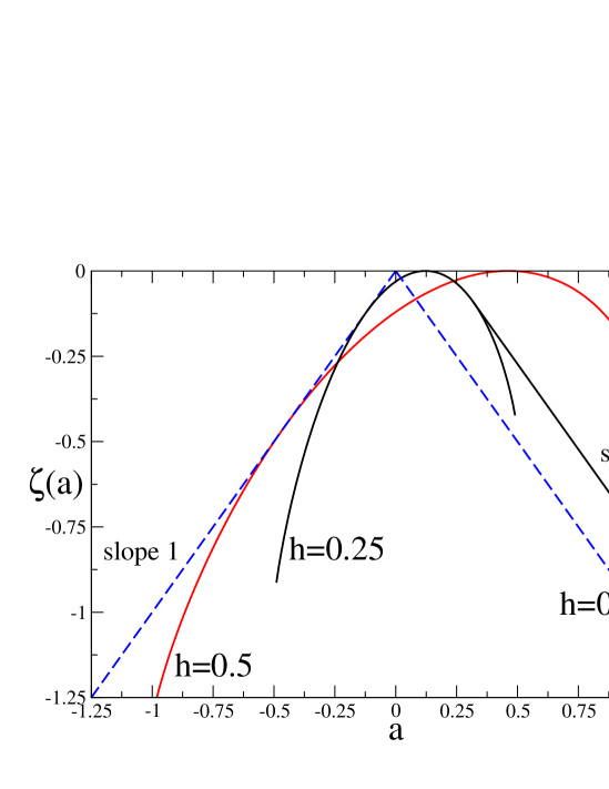
Figure 4.2: An example in a stochastic model. The graph gives the two functions $\widetilde{\zeta}_{0}(a)$ and $\widetilde{\zeta}(a)$ for $h=0.,0.25,0.5$. The average of $a$ is $\left\langle a\right\rangle=\sigma_{+}=2h\tanh h$, $a_{+}=2h\tanh 3h$ and $a^{*}=2h$. The function $\widetilde{\zeta}(a)$ is obtained from $\widetilde{\zeta}_{0}(a)$ by continuing it for $a<a_{-}=-\sigma_{+}$ and $a>a_{+}$ with straight lines of slope $\pm 1$. It does not satisfy the fluctuation relation for $|a|>\left\langle a\right\rangle$. As $h\rightarrow 0$, $\left\langle a\right\rangle\rightarrow 0$, which means that the interval in which the fluctuation relation is verified shrinks to $0$. In this limit $a_{+}\rightarrow 0$, so $\widetilde{\zeta}(a)$ approaches $-|a|$ (dashed lines). Rephrasing this in terms of $p=\frac{a}{\left\langle a\right\rangle}$ one obtains that the fluctuation relation remains always valid for $|p|<1$, even as $h\rightarrow 0$. The three curves for $\widetilde{\zeta}_{0}(a)$ have the same tangent on left side. The function $\widetilde{\zeta}_{0}(a)$ is finite only in the interval $[-2h,2h]$ and it is $-\infty$ outside it, while the function $\widetilde{\zeta}(a)$ is finite for all $a$’a and is a straight line outside $[a_{-},a_{+}]$.

It follows that, if $\widetilde{\zeta}_{0}(a_{0})$ satisfies the fluctuation relation up to $a=p^{*}\sigma_{+}$, then $\widetilde{\zeta}(a)$ satisfies the fluctuation relation only in the interval $|a|<|a_{-}|=\sigma_{+}$. Outside this interval $\widetilde{\zeta}(a)$ does not satisfy the fluctuation relation and in particular for $a\geq a_{+}$ it is $\widetilde{\zeta}(a)-\widetilde{\zeta}(-a)=const.$, as already described in [120]. Translated into the normalized variables $p_{0}=a_{0}/\sigma_{+}$ and $p=a/\sigma_{+}$, this means that, even if the large deviation function of $p_{0}$ satisfies the fluctuation relation up to $p^{*}>1$, the large deviation function of $p$ verifies the fluctuation relation only for $|p|\leq 1$. This effect is due to the presence of the singular boundary term.

An example of $\widetilde{\zeta}(a)$ is reported in Fig. 4.2: it is a simple stochastic model for the FT (taken from [95], see also the extensions in [108, 121]). The example is the Ising model without interaction in a field $h$, i.e. a Bernoulli scheme with symbols $\pm$ with probabilities $p_{\pm}=\frac{e^{\pm h}}{2\cosh h}$. Defining $a_{0}=\frac{1}{\tau}\sum_{i=0}^{\tau-1}2h\sigma_{i}$, so that $\sigma_{+}=\langle a_{0}\rangle=2h\tanh h$, and setting $x\equiv\frac{1+a_{0}/(2h)}{2}$, and $s(x)=-x\log x-(1-x)\log(1-x)$, one computes $\widetilde{\zeta}_{0}(a_{0})=s(x)+\frac{1}{2}a_{0}+const$ which is not Gaussian and it is defined in the interval $[-a^{*},a^{*}]$ with $a^{*}=2h$. In this case the large deviation function $\widetilde{\zeta}_{0}(a_{0})$ satisfies the fluctuation relation for $|a_{0}|\leq a^{*}$. If a singular term $V=-\log(\sum_{i=0}^{\infty}2^{-i-1}\frac{\sigma_{i}+1}{2})$ is added to $a_{0}$, defining $a=a_{0}+\beta(V_{i}-V_{f})$ (with $\beta=\log_{2}(1+e^{2h})$ so that the probability distribution of $V$ is $\sim e^{-\beta V}$ for large $V$), the resulting $\widetilde{\zeta}(a)$ does not verify the fluctuation relation for $a>\left\langle a\right\rangle=2h\tanh h$. In particular, for $h\rightarrow 0$, the interval in which the fluctuation relation is satisfied vanishes.

How to remove singularities

From the discussion above it turns out that singular terms which are proportional to total derivatives of unbounded functions (like the term $\frac{dV}{dt}$ that appears in the phase space contraction rate of isokinetic systems) can induce “undesired” (or “unphysical”) modifications of the large deviation function $\zeta(p)$.

On heuristic grounds, when dealing with singular systems, one could follow the prescription that unbounded terms in $\sigma(x)$ which are proportional to total derivatives should be subtracted from the phase space contraction rate. If the resulting $\sigma(x)$ is bounded (as it is e.g. for the isokinetic thermostat) then its distribution should verify the fluctuation relation for $|p|\leq p^{*}$, $p^{*}$ being an intrinsic dynamic quantity defined by $\lim_{|p|\rightarrow p^{*}}\zeta(p)=-\infty$. If the singular terms are not subtracted, the fluctuation relation will appear to be valid only for $|p|\leq 1$ even if $p^{*}>1$.

The heuristic prescription above can be motivated by a careful analysis of the proof of the fluctuation theorem for Anosov flows. In the following let us call again $a$ the integral of the total phase space contraction rate $\sigma(x)$ (which includes singular terms) and $a_{0}$ the integral of the bounded variable $\sigma_{0}(x)$ from which singular total derivatives have been removed.

The fluctuation theorem was proved in [122] for Anosov flows. Flows are associated with maps via Poincaré’s sections: excluding singular sections which pass through a point of singularity in phase space (which is a very natural restriction) the chaotic hypothesis would lead to a fluctuation relation for the phase space contraction on a Poincaré’s section and this would lead to a fluctuation relation for the flow by the theory in [122] only if the variable $\sigma(x)$ is bounded. However if the Poincaré’s section is performed avoiding the singular points, like the passage through points in which the potential is infinite, then the phase space contraction (taken for instance assuming as timing events the instants in which the potential energy exceeds some large value) has two contributions: the first is from $a_{0}$ which is bounded (at least in the isokinetic thermostats) and the second from the potential. The latter however has again the form proportional to the difference of the potential energy at the initial timing event and at the final event: this vanishes on the section considered above while in general it will have the form of $\frac{1}{\tau}$ times a bounded quantity (unless the section passes through a singularity of the potential). Therefore the distribution of $a_{0}$ will satisfy the fluctuation relation (by the chaotic hypothesis) for $|a_{0}|<p^{*}\sigma_{+}$. By the above maximum argument, the distribution of $a$ will also verify, as a consequence, the fluctuation relation but only for $|a|\leq\sigma_{+}$ (i.e. for $|p|\leq 1$).

The (natural) prescription is then to consider only Poincaré’s sections which do not pass through a singularity of $\sigma(x)$. The integral of $\sigma(x)$ over a large number of timing events on such sections is equal to the time integral of $\sigma_{0}(x)$ plus a bounded term which can be neglected. Thus the prescription on the Poincaré’s section is equivalent to the heuristic prescription of removing from $\sigma(x)$ all the unbounded total derivatives.

It follows that the chaotic hypothesis leads to a prediction on the outcome of possible numerical simulations in which the isokinetic thermostat is assumed in particle systems interacting via a Lennard–Jones potential: the fluctuation relation will hold for all $|a|\leq\sigma_{+}$ and, once the term $\frac{dV}{dt}$ is removed, for all $|a_{0}|<p^{*}\sigma_{+}$ with $p^{*}\geq 1$, even for the latter models which admittedly are quite unphysical as the speed of the particles remains essentially constant even in “head on” collisions in which the potential energy acquire an infinite value. The numerical results of the following chapter [100, 102] closely agree with this prediction and can be considered as rather demanding tests of it.

4.4.4 Some remarks on the chaotic hypothesis

(1) It has to be stressed that the chaotic hypothesis concerns physical systems: it is very easy to find dynamical systems for which it does not hold. As it is easy (actually even easier) to find systems in which the ergodic hypothesis does not hold (e.g. harmonic lattices or black body radiation) but, if suitably interpreted, leads to physically correct results (the specific heats at high temperature) or, when it really fails, to new scientific paradigms (like quantum mechanics from the specific heats at low temperature and Planck’s law).

(2) Since physical systems are almost always not Anosov systems it is very likely that probing motions in extreme regimes (e.g. when particles go undisturbed through infinite potential walls, as in the Lennard–Jones isokinetic models) will make visible the features that distinguish Anosov systems from non Anosov systems: e.g. the isokinetic thermostats satisfy the fluctuation relation for $|p|\leq 1$ only (if the term $\frac{dV}{dt}$ is not removed from $\sigma(x)$). Note that this results can be derived from the chaotic hypothesis as discussed above: this is a quite remarkable fact.

(3) If the term $\frac{dV}{dt}$ is removed (as will be done in the following), the resulting quantity $\sigma_{0}(x)$ is bounded and its distribution verifies the fluctuation relation also for $|p|>1$. This prescription, as discussed above, is equivalent to the very reasonable prescription that the Poincaré’s section used for mapping the flow into a map does not pass through a singularity of $\sigma(x)$.

4.5 Appendix: The large deviation function of $\sigma(x)$ close to equilibrium

Close to equilibrium the entropy production rate has the form $\sigma(t)=E{\cal J}(t)$, as discussed in section 4.4.1. Thus, from Eq. (4.32),

$$z^{(k)}_{\infty}=(-1)^{k-1}\lim_{\tau\rightarrow\infty}\tau^{-1}\left\langle\sigma_{\tau}^{k}\right\rangle_{c}=(-1)^{k-1}E^{k}\lim_{\tau\rightarrow\infty}\tau^{-1}\int_{-\tau/2}^{\tau/2}dt_{1}\cdots\int_{-\tau/2}^{\tau/2}dt_{k}\left\langle{\cal J}(t_{1})\cdots{\cal J}(t_{k})\right\rangle_{c}\ .$$ (4.45)

The connected correlations $\left\langle{\cal J}(t_{1})\cdots{\cal J}(t_{k})\right\rangle_{c}$ are translationally invariant due to the stationarity of the SRB distribution and decay exponentially in the differences $|t_{i}-t_{j}|$ due to the short range property of the SRB potentials.

From stationarity it follows that $z^{(1)}_{\infty}=E\left\langle{\cal J}\right\rangle$ and as $\left\langle{\cal J}\right\rangle=0$ in equilibrium, one has $\left\langle{\cal J}\right\rangle\sim E$ and $z^{(1)}_{\infty}=\sigma_{+}\sim E^{2}$. Using stationarity and the exponential decay of the connected correlations one has, for $k>1$,

$$\begin{split}\lim_{\tau\rightarrow\infty}\tau^{-1}\int_{-\tau/2}^{\tau/2}dt_{1}&\cdots\int_{-\tau/2}^{\tau/2}dt_{k}\left\langle{\cal J}(t_{1})\cdots{\cal J}(t_{k})\right\rangle_{c}=\\ =&\int_{-\infty}^{\infty}dt_{1}\cdots\int_{-\infty}^{\infty}dt_{k-1}\left\langle{\cal J}(0){\cal J}(t_{1})\cdots{\cal J}(t_{k-1})\right\rangle_{c}\equiv{\cal J}^{(k)}_{\infty}\ ,\end{split}$$ (4.46)

and the ${\cal J}^{(k)}_{\infty}$ are finite for $E\rightarrow 0$. This means that the $z_{\infty}^{(k)}\sim E^{k}$ for $k>1$ and

$$z_{\infty}(\lambda)=z_{\infty}^{(1)}\lambda+\frac{z_{\infty}^{(2)}}{2}\lambda^{2}+O(E^{3}\lambda^{3})\ .$$ (4.47)

Equivalently, from the relation $\zeta_{\infty}(p)=\min_{\lambda}[\lambda p\sigma_{+}-z_{\infty}(\lambda)]$ one can prove that

$$\zeta_{\infty}(p)=\frac{\sigma_{+}^{2}}{2z_{\infty}^{(2)}}(p-1)^{2}-\frac{z_{\infty}^{(3)}\sigma_{+}^{3}}{6\big{(}z_{\infty}^{(2)}\big{)}^{3}}(p-1)^{3}+\ldots=\frac{\sigma_{+}^{2}}{2z_{\infty}^{(2)}}(p-1)^{2}+O(E^{3}(p-1)^{3})\ ,$$ (4.48)

i.e. that $\zeta_{\infty}(p)$ is approximated by a Gaussian in an interval $|p-1|\sim 1/E$ whose size grows for $E\rightarrow 0$, see also [109].

Chapter 5 Numerical tests of the Fluctuation Relation

5.1 Introduction

As discussed in section 4.4.1, close to equilibrium the pdf of the phase space contraction rate is close to a Gaussian, and the fluctuation relation is equivalent to the Green-Kubo relations obtained within linear response theory. Thus, a test of the fluctuation relation in this context is not really independent from linear response theory.

A rather stringent test of the chaotic hypothesis would be a check which cannot be reduced to a kind of Green-Kubo relation; this requires at least one of the two following conditions to be satisfied:

1. the distribution $\pi_{\tau}(p)$ is distinguishable from a Gaussian, or

2. deviations from the leading order in $E$ in Eq. (4.38), i.e. deviations from the Green-Kubo relation, are observed.

This is very hard to obtain in numerical simulations of Eq. (4.4) for the following reasons:

1. to observe deviations from linearity in Eq. (4.38) one has to apply very large forces $E$, then $\sigma_{+}$ is very large and it becomes very difficult to observe the negative values of $p(x)$ that are needed to compute $\zeta_{\infty}(-p)$ in Eq. (4.11);

2. deviations from Gaussianity in $\pi_{\tau}(p)$ are observed only for values of $p$ that differ significantly (of the order of $2$ times the variance) from $1$ and, again, it is very difficult to observe such values of $p$.

Due to the limited computational resources available in the past decade, all numerical computations that can be found in the literature on systems described by Eq. (4.4) found that the measured distribution $\pi_{\tau}(p)$ could not be distinguished from a Gaussian distribution in the interval of $p$ accessible to the numerical experiment [94, 95, 96, 100].

In this chapter a test of the fluctuation relation, in a numerical simulation of a system described by Eq. (4.4), for large applied force when deviations from linearity can be observed, and the distribution $\pi_{\tau}(p)$ is appreciably non-Gaussian, will be presented [102]. This has become possible thanks to the fast increase of computational power in the last decade. However, it is still very difficult to reach values of $\tau$ which can be confidently regarded as “close” to the asymptotic limit $\tau\rightarrow\infty$; thus to interpret the results a theory of the $o(1)$ corrections to the function $\zeta_{\infty}(p)$ has to be developed in order to extract the limiting function $\zeta_{\infty}(p)$ from the numerical data. Taking into account the latter finite time corrections, the fluctuation relation will be successfully tested for non–Gaussian distributions and beyond the linear response theory. A similar analysis has been presented in [123], where however negative values of $p$ were not directly observed.

5.2 Finite time corrections to the Fluctuation Relation

In the present section a strategy to study (in principle constructively) the $O(1)$ corrections in the exponent of Eq. (4.10) will be described. The theory holds assuming that the time evolution is hyperbolic so that it can be applied to physical systems only if the chaotic hypothesis is accepted. For simplicity only the case of discrete time evolution via a map $S$ are considered.

5.2.1 Finite time corrections to the characteristic function

The distribution of $p$ at fixed $\tau$ can be studied via its Laplace transform (characteristic function) $z_{\tau}(\lambda)$:

$$z_{\tau}(\lambda)=-\frac{1}{\tau}\log\langle e^{-\lambda\sum_{j=0}^{\tau-1}\sigma(S^{j}x)}\rangle\ .$$ (5.1)

From the explicit expression of the SRB measure, see Eq. (4.20), it can computed as

$$e^{-\tau z_{\tau}(\lambda)}=\lim_{T\rightarrow\infty}\frac{\sum_{\underline{\varepsilon}}e^{-\sum_{X\subset\Lambda_{T}}\Phi_{+}(\underline{\varepsilon}_{X})-\lambda\,\sum_{X\circ\,[0,\tau-1]}s(\underline{\varepsilon}_{X})}}{\sum_{\underline{\varepsilon}}e^{-\sum_{X\subset\Lambda_{T}}\Phi_{+}(\underline{\varepsilon}_{X})}}\ .$$ (5.2)

This means that it is the (limit as $T\rightarrow\infty$ of the) ratio between the partition functions $Z_{T}(\Phi_{+})$ of a Gibbs distribution in $\Lambda_{T}$ with potential $\Phi_{+}$ (the denominator) and the partition function $Z_{T}(\Phi_{+},\lambda s)$ with the same potential modified in the finite region $[0,\tau-1]\subset\hbox{\msytw Z}$ by the addition of a potential $\lambda s(\underline{\varepsilon}_{X})$.

The one dimensional systems are very well understood and the above is a well studied problem in statistical mechanics, known as a finite size corrections calculation. For instance it can be attacked by cluster expansion [91]; this is a technique to deal with the average of the exponential of a spin Hamiltonian which is defined in terms of potentials $\phi$ exponentially decaying with rate $\kappa$, such as those appearing in the numerator and in the denominator of Eq. (5.2). It allows us to represent them as:

$$\sum_{\underline{\varepsilon}}e^{-\sum_{X\subset\Lambda_{T}}\phi({\underline{\varepsilon}}_{X})}=e^{-\sum_{X\subset\Lambda_{T}}\widetilde{\phi}_{X}}\;,$$ (5.3)

where $\widetilde{\phi}_{X}$ are new effective potentials, explicitly computable in terms of suitable averages of products of $\phi({\underline{\varepsilon}}_{X})$’s, and which can be proven to be still exponentially decaying with the diameter of $X$ with a rate $0<\kappa^{\prime}\leq\kappa$.

In particular, a representation like Eq. (5.3) allows to rewrite the partition function in the denominator of Eq. (5.2) as:

$$Z_{T}(\Phi_{+})=\exp\left[(2T+1)f_{\infty}(\Phi_{+})-c_{\infty}(\Phi_{+})+O(e^{-\kappa^{\prime}T})\right]\ ,$$ (5.4)

and the one in the numerator as

$$Z_{T}(\Phi_{+},\lambda s)=\exp\Big{[}(2T+1-\tau)f_{\infty}(\Phi_{+})+\tau f_{\infty}(\Phi_{+}+\lambda s)-c_{\infty}(\Phi_{+})-g_{\infty}(\lambda)+O(e^{-\kappa^{\prime}T}+e^{-\kappa^{\prime}\tau})\Big{]}\ .$$ (5.5)

Therefore

$$z_{\tau}(\lambda)=f_{\infty}(\Phi_{+})-f_{\infty}(\Phi_{+}+\lambda s)+\frac{g_{\infty}(\lambda)}{\tau}+O(e^{-\kappa^{\prime}\tau})\equiv z_{\infty}(\lambda)+\frac{g_{\infty}(\lambda)}{\tau}+O(e^{-\kappa^{\prime}\tau})\ .$$ (5.6)

The function $z_{\infty}(\lambda)$ is convex in $\lambda$ and the functions $g_{\infty}(\lambda)$ and $z_{\tau}(\lambda)$ are analytic in $\lambda$ (a consequence of the $1$-dimensionality and of the short range nature of the SRB distribution): namely $g_{\infty}(\lambda)=g^{(1)}_{\infty}\lambda+\frac{1}{2}g^{(2)}_{\infty}\lambda^{2}+\ldots$ and $z_{\tau}(\lambda)=z^{(1)}_{\tau}\lambda+\frac{1}{2}z^{(2)}_{\tau}\lambda^{2}+\ldots$ and the coefficients of their expansion in a power series of $\lambda$ can be expressed in terms of correlation functions of $\sigma(x)$. For instance, from Eq. (5.1) and using the translational invariance of the SRB measure,

$$\begin{split}z^{(1)}_{\tau}&=\tau^{-1}\langle\sum_{j=0}^{\tau-1}\sigma(S^{j}x)\rangle=\sigma_{+}\ ,\\ z^{(2)}_{\tau}&=\tau^{-1}\left[\langle\sum_{j=0}^{\tau-1}\sigma(S^{j}x)\rangle^{2}-\langle\sum_{j=0}^{\tau-1}\sigma(S^{j}x)\sum_{k=0}^{\tau-1}\sigma(S^{k}x)\rangle\right]\\ &=-\sum_{k=-\tau+1}^{\tau-1}\left[1-\frac{|k|}{\tau}\right]\langle\sigma(S^{k}x)\sigma(x)\rangle_{c}\ ,\end{split}$$ (5.7)

where $\langle\sigma(S^{k}x)\sigma(x)\rangle_{c}=\langle\sigma(S^{k}x)\sigma(x)\rangle-\sigma_{+}^{2}$. Using Eq. (5.6), $g_{\infty}(\lambda)=\lim_{\tau\rightarrow\infty}\tau[z_{\tau}(\lambda)-z_{\infty}(\lambda)]$, and the analyticity of $z_{\tau}(\lambda)$, one has $g^{(j)}_{\infty}=\lim_{\tau\rightarrow\infty}\tau[z^{(j)}_{\tau}-z^{(j)}_{\infty}]$. Since the connected correlation function $\langle\sigma(S^{k}x)\sigma(x)\rangle_{c}$ decays exponentially for $k\rightarrow\infty$, one obtains

$$\begin{split}&g^{(1)}_{\infty}=0\ ,\\ &g^{(2)}_{\infty}=\sum_{k=-\infty}^{\infty}|k|\langle\sigma(S^{k}x)\sigma(x)\rangle_{c}\ .\end{split}$$ (5.8)

5.2.2 Finite time corrections to $\zeta_{\infty}(p)$

A direct measurement of $z_{\tau}(\lambda)$ from the numerical data is difficult. What is really accessible to numerical observation are the quantities $\frac{1}{\tau}\log\pi_{\tau}(\{p\in\Delta\})$ in Eq. (4.10) because the measured values of $p$ are used to build an histogram obtained by dividing the $p$–axis into sufficiently small bins $\Delta$ and counting how many values of $p$ fall in the various bins. The size of the bins $\Delta$ will be chosen to be $|\Delta|=O(\varepsilon_{\tau}/\tau)$, with $\varepsilon_{\tau}$ a small parameter which will be eventually chosen $\varepsilon_{\tau}=o(1)$, see Appendix 5.8 for a discussion of this point. Let also $p_{\Delta}$ be the center of the bin $\Delta$. An application of a local form of central limit theorem, discussed in Appendix 5.8, shows that the following asymptotic representation of $\pi_{\tau}(\{p\in\Delta\})$ holds:

$$\pi_{\tau}(\{p\in\Delta\})=e^{\tau\zeta_{\tau}(p_{\Delta})}\Big{(}1+o(1)\Big{)}\ ,$$ (5.9)

where $\zeta_{\tau}(p_{\Delta})$ can be interpolated by an analytic function of $p$, satisfying the equation

$$\zeta_{\tau}(p)=-z_{\tau}(\lambda_{p})+\lambda_{p}p\sigma_{+}-\frac{1}{2\tau}\log\left[\frac{2\pi}{\tau}\Big{(}-\frac{z_{\tau}^{\prime\prime}(\lambda_{p})}{\sigma_{+}^{2}}\Big{)}\right]\ ,$$ (5.10)

and $\lambda_{p}$ is the inverse of $p(\lambda)=z_{\tau}^{\prime}(\lambda)/\sigma_{+}$. Using the previous equations, the lowest order finite time correction to $\zeta_{\infty}(p)$ around the maximum can be computed.

First one rewrites $\zeta_{\tau}(p)$ as $\zeta_{\tau}(p)=\zeta_{\infty}(p)+\frac{\gamma_{\infty}(p)}{\tau}+O(\frac{1}{\tau^{2}})$. By the analyticity of $\zeta_{\tau}(p)$, one can write $\zeta_{\infty}(p),\gamma_{\infty}(p)$ around $p=1$ in the form: $\zeta_{\infty}(p)=\frac{1}{2}\zeta_{\infty}^{(2)}(p-1)^{2}+\frac{1}{3!}\zeta_{\infty}^{(3)}(p-1)^{3}+\ldots$ and $\gamma_{\infty}(p)=\gamma_{\infty}^{(0)}+\gamma_{\infty}^{(1)}(p-1)+\ldots$.

Up to terms of order $(p-1)^{2}$ and higher in the series for $\gamma_{\infty}(p)$, one has:

$$\begin{split}\zeta_{\tau}(p)&=\zeta_{\infty}(p)+\frac{\gamma_{\infty}^{(0)}}{\tau}+\frac{\gamma_{\infty}^{(1)}}{\tau}(p-1)+O\left(\frac{(p-1)^{2}}{\tau}\right)+o\left(\frac{1}{\tau}\right)=\\ &=\zeta_{\infty}\left(p+\frac{\gamma_{\infty}^{(1)}}{\tau\zeta^{(2)}_{\infty}}\right)+\frac{\gamma_{\infty}^{(0)}}{\tau}+O\left(\frac{(p-1)^{2}}{\tau}\right)+o\left(\frac{1}{\tau}\right)\;.\end{split}$$ (5.11)

Thus, the finite time corrections to $\zeta_{\infty}(p)$ around its maximum begin with a shift of the maximum at

$$p_{0}=1-\frac{\gamma^{(1)}_{\infty}}{\tau\zeta^{(2)}_{\infty}}+o\left(\frac{1}{\tau}\right)\ .$$ (5.12)

To apply the latter result one needs to compute $\gamma^{(1)}_{\infty}$ in terms of observable quantities. And, in order to compute $\gamma^{(1)}_{\infty}$ one can apply Eq. (5.10). First of all, note that $\lambda_{p}$ is determined by the condition

$$p\sigma_{+}=z^{\prime}_{\tau}(\lambda_{p})=\sigma_{+}+z_{\tau}^{\prime\prime}(0)\lambda_{p}+O(\lambda_{p}^{2})\ ,$$ (5.13)

where Eq. (5.7) and Eq. (5.8) have been used. Then, $\lambda_{p}=\frac{\sigma_{+}(p-1)}{z_{\tau}^{\prime\prime}(0)}+O\big{(}(p-1)^{2}\big{)}$. Substituting this result into Eq. (5.10) and equating the terms of order $O(\frac{p-1}{\tau})$ at both sides one finds:

$$\gamma_{\infty}^{(1)}=-\frac{1}{2}\frac{z_{\infty}^{(3)}\sigma_{+}}{(z_{\infty}^{(2)})^{2}}\;.$$ (5.14)

The last equation can also be rewritten as:

$$\gamma_{\infty}^{(1)}=\frac{\zeta_{\infty}^{(3)}}{2\zeta_{\infty}^{(2)}}\ .$$ (5.15)

This can be proven recalling that $\zeta_{\infty}^{(2)}$ and $\zeta_{\infty}^{(3)}$ are derivatives of $\zeta_{\infty}(p)$ in $p=1$, that can be obtained by differentiating w.r.t. $\lambda$ (two or three times, respectively) the definition $\zeta_{\infty}\big{(}z_{\infty}^{\prime}(\lambda)/\sigma_{+}\big{)}=-z_{\infty}(\lambda)+\lambda z_{\infty}^{\prime}(\lambda)$ and computing the derivatives in $\lambda=0$ recalling that $z_{\infty}^{\prime}(0)/\sigma_{+}=1$. Plugging Eq. (5.15) into Eq. (5.12) one finally gets

$$p_{0}=1-\frac{\zeta^{(3)}_{\infty}}{2\tau(\zeta^{(2)}_{\infty})^{2}}+o\left(\frac{1}{\tau}\right)\ ,$$ (5.16)

that is the main result of this section. The key point is that the moments $\zeta_{\infty}^{(2)}$ and $\zeta_{\infty}^{(3)}$ in Eq. (5.16) are quantities that can be measured from the numerical data (within an $O(\tau^{-1})$ error). One then has a verifiable prediction on the expected shift of the maximum at finite $\tau$. The data agree very well with this prediction, see Fig. 5.1 and corresponding discussion in section 5.4 below.

Substituting Eq. (5.16) in Eq. (5.11), one finally finds:

$$\zeta_{\infty}(p)=\eta_{\tau}(p)+O\Big{(}\frac{(p-1)^{2}}{\tau}\Big{)}+o(\tau^{-1})\;,$$ (5.17)

where $\eta_{\tau}(p)$ is defined as

$$\eta_{\tau}(p)\equiv-\frac{\gamma^{(0)}_{\infty}}{\tau}+\zeta_{\tau}\left(p-\frac{\zeta_{\infty}^{(3)}}{2\tau(\zeta_{\infty}^{(2)})^{2}}\right)\;.$$ (5.18)

The key point of the above discussion was the validity of Eq. (5.9–5.10); see Appendix 5.8 for their derivation.

5.2.3 Remarks

(1) The shift away from $1$ of the maximum of the function $\zeta_{\tau}(p)$ at finite $\tau$, expressed by the second term in Eq. (5.18), is due to the asymmetry of the distribution $\pi_{\tau}(p)$ around the average value $p=1$; consequently, it is proportional, at leading order in $\tau^{-1}$, to $\zeta_{\infty}^{(3)}$ which is indeed a measure of the asymmetry of $\zeta_{\infty}(p)$ around $p=1$. This shift would be absent in the case of a symmetric distribution (e.g. a Gaussian) and for this reason it was not observed in previous experiments [94, 95, 96, 100].

(2) The error term in the r.h.s. of Eq. (5.9) is $o(1)$ w.r.t. $\tau$ and it does not affect the computation of $\gamma_{\infty}(p)$. It is then clear that with a calculation similar to that performed above, one can get equations for the coefficients $O(\lambda^{k})$ in the exponents of Eq. (5.9); in this way one can iteratively construct the whole sequence of coefficients $\gamma_{\infty}^{(k)}$ defining the power series expansion of $\gamma_{\infty}(p)$.

(3) In models with continuous time evolution the quantity $\sigma_{+}$ is not dimensionless but it has dimensions of inverse time: in such cases one can imagine that one is still studying a map which maps a system configuration at a time when some prefixed event happens in the system (typically a “collision”) into the next one in which a similar event takes place. If $\tau_{0}$ is the average time interval between such events then $\tau_{0}\sigma_{+}$ will play the role played by $\sigma_{+}$ in the discrete time case: it will be the adimensional parameter entering the estimates of the error terms.

Note that the coefficients $g_{\infty}^{(k)}$ are of order $\sigma_{+}^{k}$, and their size is necessarily estimated by the adimensional entropy production to the $k$–th power. Then, in the continuous time case, the choice of $\tau_{0}$ affects the estimates of the remainders, because it affects the size of the adimensional parameter $\tau_{0}\sigma_{+}$; and the size of the mixing time (that is connected with the estimated range of decay of the potentials, see [91]). The natural (and physical) choice for $\tau_{0}$ is the mixing time. Consistently with this remark, at the moment of constructing numerically the distribution function for the entropy production rate averaged over a time $\tau$, time intervals of the form $\tau=\tau_{0}n$, $n\geq 1$, will be considered, see section 5.3.3 below.

5.3 Models

The model that will be considered in the following is a system of $N$ classical particles of equal mass $m$ in dimension $d$; they are described by their position $q_{i}$ and momenta $p_{i}=m\dot{q}_{i}$, $(p_{i},q_{i})\in R^{2d},\ i=1,\ldots,N$. The particles are confined in a cubic box of side $L$ with periodic boundary conditions. Each particle is subject to a conservative force, $f_{i}({\underline{q}})=-\partial_{q_{i}}V({\underline{q}})$, and to a nonconservative force $E_{i}$ that does not depend on the phase space variables. The force $E_{i}$ is locally conservative but not globally such due to periodic boundary conditions. The mechanical thermostat is a Gaussian thermostat [80], $\theta_{i}({\underline{p}},{\underline{q}})=-\alpha({\underline{p}},{\underline{q}})\,p_{i}$, and the function $\alpha({\underline{p}},{\underline{q}})$ is defined by the condition that the total kinetic energy $K({\underline{p}})\equiv\frac{1}{2m}|{\underline{p}}|^{2}=\frac{1}{2m}\sum_{i}p^{2}_{i}$ should be a constant (isokinetic ensemble). The equations of motion are:

$$\begin{cases}&\dot{q}_{i}=\frac{p_{i}}{m}\ ,\\ &\dot{p}_{i}=f_{i}({\underline{q}})+E_{i}-\alpha({\underline{p}},{\underline{q}})\ p_{i}\ ,\end{cases}$$ (5.19)

and are a particular instance of Eq. (4.4). From the constraint $\frac{dK}{dt}=0$ one obtains

$$\alpha({\underline{p}},{\underline{q}})=\frac{\sum_{i}E_{i}\ p_{i}+\sum_{i}f_{i}({\underline{q}})\ p_{i}}{\sum_{i}p^{2}_{i}}\ .$$ (5.20)

5.3.1 Entropy production rate

The total phase space volume contraction rate for this system is given by:

$$\begin{split}&\sigma({\underline{p}},{\underline{q}})=-\sum_{i}\left(\frac{\partial\dot{q}_{i}}{\partial q_{i}}+\frac{\partial\dot{p}_{i}}{\partial p_{i}}\right)=dN\alpha({\underline{p}},{\underline{q}})+\sum_{i}\frac{\partial\alpha}{\partial p_{i}}p_{i}=(dN-1)\ \alpha({\underline{p}},{\underline{q}})\ .\end{split}$$ (5.21)

Defining the kinetic temperature, $T\equiv 2K({\underline{p}})/(dN-1)$, [80], the phase space contraction rate can be rewritten as

$$\sigma({\underline{p}},{\underline{q}})=\frac{\sum_{i}E_{i}\ \dot{q}_{i}-\dot{V}}{T}\ .$$ (5.22)

The first term is the power dissipated by the external force divided by the kinetic temperature, and can be identified with the entropy production rate, see the discussion in section 4.4 and [80, 84, 94]. The second term is the total derivative w.r.t. time of the potential energy divided by the temperature: following the discussion of section 4.4.3 this term will be removed, and the distribution of the entropy production rate $\dot{s}$, where $\dot{s}$ is identified with $\sigma$ minus the total derivative term $-\dot{V}/T$ in Eq. (5.22), will be studied:

$$\dot{s}({\underline{p}},{\underline{q}})=\frac{\sum_{i}E_{i}\ \dot{q}_{i}}{T}\ .$$ (5.23)

From now on $\zeta_{\infty}(p)$ and $\zeta_{\tau}(p)$ will be the distributions for the fluctuations of the entropy production rate $\dot{s}$ averaged over infinite or finite time, respectively. These will be the objects that will be measured and used from now on.

In order to define the current ${\cal J}(x,E)$, it is useful to rewrite $E_{i}=E\,u_{i}$, where $u_{i}$ is a (constant) unit vector that specifies the direction of the force acting on the $i$-th particle. Then, according to Eq. (4.37),

$${\cal J}({\underline{p}},{\underline{q}})=\frac{\partial\sigma}{\partial E}=\frac{\sum_{i}u_{i}\,\dot{q}_{i}}{T}\ .$$ (5.24)

5.3.2 Discretization of the equations of motion

To perform the numerical simulation, one has to write the equations of motion in a discrete form. One possibility is to use the Verlet algorithm [124]; for Hamiltonian equations of motion (i.e., ${\underline{E}}={\underline{0}}$ and $\alpha=0$)

$$\begin{cases}&\dot{q}_{i}=\frac{p_{i}}{m}\ ,\\ &\dot{p}_{i}=f_{i}({\underline{q}})\ ,\end{cases}$$ (5.25)

the Verlet discretization has the form

$$\begin{cases}&q_{i}(t+dt)=q_{i}(t)+\frac{p_{i}(t)}{m}dt+\frac{1}{2}f_{i}(t)dt^{2}\ ,\\ &p_{i}(t+dt)=p_{i}(t)+\frac{1}{2}\big{[}f_{i}(t)+f_{i}(t+dt)\big{]}dt\ ,\end{cases}$$ (5.26)

where $dt$ is the time step size. This discretization ensures that the error is $O(dt^{4})$ on the positions $q_{i}(t)$ in a single time step. The implementation of this algorithm on a computer is discussed in detail in [124].

However, this method requires the forces $f_{i}(t)$ to depend only on the positions and not on the velocities: hence, it has to be adapted to Eq.s (5.19). This has been done in the following way. The discretized equations are written as

$$\begin{cases}q_{i}(t+dt)&=q_{i}(t)+\frac{p_{i}(t)}{m}dt+\frac{1}{2}\big{[}f_{i}(t)+E_{i}-\alpha(t)p_{i}(t)\big{]}dt^{2}\ ,\\ p_{i}(t+dt)&=p_{i}(t)+E_{i}+\frac{1}{2}\big{[}f_{i}(t)+f_{i}(t+dt)-\alpha(t)p_{i}(t)-\alpha(t+dt)p_{i}(t+dt)\big{]}dt\ ,\end{cases}$$ (5.27)

with the same error as in the standard Verlet discretization. At time $t$, the positions $q_{i}(t)$, the momenta $p_{i}(t)$, the forces $f_{i}(t)$, and the Gaussian multiplier $\alpha(t)$ are stored in the computer. Then, the following operations are performed:

1. the new positions $q_{i}(t+dt)$ are calculated using the first equation;

2. using the new positions, the new forces $f_{i}(t+dt)$ are calculated (the conservative forces depend only on the positions);

3. the quantity $\xi_{i}=p_{i}(t)+E_{i}+\frac{1}{2}\big{[}f_{i}(t)+f_{i}(t+dt)-\alpha(t)p_{i}(t)\big{]}dt$ is calculated; note that $p_{i}(t+dt)$ can be expressed in terms of the (known) $\xi_{i}$ and the (unknown) $\alpha(t+dt)$ as

   $$p_{i}(t+dt)=\frac{\xi_{i}}{1-\alpha(t+dt)dt/2}\ ;$$ (5.28)

4. substituting Eq. (5.28) in the definition of $\alpha(t+dt)$, Eq. (5.20), a self-consistency equation for $\alpha(t+dt)$ is obtained, whose solution is

   $$\begin{split}&\alpha(t+dt)=\frac{\alpha_{0}}{1-\alpha_{0}dt/2}\ ,\\ &\alpha_{0}=\frac{\sum_{i}E_{i}\ \xi_{i}+\sum_{i}f_{i}(t+dt)\ \xi_{i}}{\sum_{i}\xi_{i}^{2}}\ ;\end{split}$$ (5.29)

5. substituting Eq. (5.29) in Eq. (5.28) $p_{i}(t+dt)$ can be calculated.

This procedure allows to calculate the new positions, momenta, forces, and $\alpha$, at time $t+dt$ according to Eq.s (5.27) without approximations, defining a map $S$ such that $({\underline{p}}(t+dt),{\underline{q}}(t+dt))=S({\underline{p}}(t),{\underline{q}}(t))$.

The simulated (discrete) dynamical system will be defined by the map $S({\underline{p}},{\underline{q}})$ and will approximate the differential equations of motion, Eq. (5.19), with error $O(dt^{4})$ for the positions and $O(dt^{3})$ for the velocities.
The map $S$ satisfies the following properties:

1. it is reversible, i.e. it exists a map $I({\underline{p}},{\underline{q}})$ (simply defined by $I({\underline{p}},{\underline{q}})=(-{\underline{p}},{\underline{q}})$) such that $IS=S^{-1}I$;

2. in the Hamiltonian case (${\underline{E}}={\underline{0}}$ and $\alpha=0$, Eq.s (5.25)) it is volume preserving.

The first property ensures that assuming the Chaotic Hypothesis the Fluctuation Relation holds for the map $S$. The second property ensures that at equilibrium the discretization algorithm conserves the phase space volume, consistently with the definition of equilibrium system which has been given in section 4.4.

5.3.3 Details of the simulation

In the simulation, the external force has been chosen of the form $E_{i}=E\,u_{i}$, where the unit vectors $u_{i}$ were parallel to the $x$ direction but with different orientation: half of them were oriented in the positive direction, and half in the negative direction, i.e. $u_{i}=(-1)^{i}\widehat{x}$, in order to keep the center of mass fixed. Two different systems have been considered, selecting interaction potentials widely used in numerical simulations (for the purpose of making easier possible future independent checks and rederivations of the results):

1. (model I) the first investigated system is made by $N=8$ particles of equal mass $m$ in $d=2$. The interaction potential is a sum of pair interactions, $V({\underline{q}})=\sum_{i<j}v(|q_{i}-q_{j}|)$, and the pair interaction is represented by a WCA potential, i.e. a Lennard-Jones potential truncated at the minimum:

   $$v(r)=\begin{cases}&4\epsilon\left[\left(\frac{\sigma}{r}\right)^{12}-\left(\frac{\sigma}{r}\right)^{6}\right]+\epsilon\ ,\hskip 10.0ptr\leq\sqrt[6]{2}\sigma\ ;\\ &0\ ,\hskip 100.0ptr>\sqrt[6]{2}\sigma\ .\end{cases}$$

   The reduced density was $\rho=N\sigma^{2}/L^{2}=0.95$ (that determines $L$), the kinetic temperature was fixed to $T=4\epsilon$ and the time step to $dt=0.001t_{0}$, where $t_{0}=\sqrt{m\sigma^{2}/\epsilon}$. In the following, all the quantities will be reported in units of $m$, $\epsilon$ and $\sigma$ (LJ units). This system was already studied in the literature, see e.g. [94, 125]. Different values of the external force $E$ were investigated, ranging from $E=0$ to $E=25$.

2. (model II) the second system is a binary mixture of $N$=20 particles (16 of type A and 4 of type B), of equal mass $m$, in $d=3$, interacting via the same WCA potential of model I; the pair potential is

   $$v_{\alpha\beta}(r)=\begin{cases}&4\epsilon_{\alpha\beta}\left[\left(\frac{\sigma_{\alpha\beta}}{r}\right)^{12}-\left(\frac{\sigma_{\alpha\beta}}{r}\right)^{6}\right]+\epsilon_{\alpha\beta}\ ,\hskip 21.0ptr\leq\sqrt[6]{2}\sigma_{\alpha\beta}\ ;\\ &0\ ,\hskip 150.0ptr>\sqrt[6]{2}\sigma_{\alpha\beta}\ ;\end{cases}$$

   $\alpha$ and $\beta$ are indexes that specify the particle species ($\alpha,\beta\in\{A,B\}$). The parameters entering the potential are the following: $\sigma_{AB}=0.8\sigma_{AA}$; $\sigma_{BB}=0.88\sigma_{AA}$; $\epsilon_{AB}=1.5\epsilon_{AA}$; $\epsilon_{BB}=0.5\epsilon_{AA}$. Similar potentials have been studied, [126, 127], as models for liquids in the supercooled regime (i.e., below the melting temperature). For this system the LJ units are $m$, $\epsilon_{AA}$, and $\sigma_{AA}$; the unit of time is then $t_{0}=\sqrt{m\sigma_{AA}^{2}/\epsilon_{AA}}$. The reduced density was $\rho=N\sigma_{AA}^{3}/L^{3}=1.2$ and the integration step was $dt=0.001t_{0}$. The unit vectors $u_{i}$ are chosen such that half of the $A$ particles and half of the $B$ particles have positive force in the $x$ direction, and the remaining particles have negative force in the $x$ direction. For this system different values of external force $E\in[0,10]$ and temperature $T\in[0.5,3]$ were investigated.

For each system and for each chosen value of $T$ and $E$, a very long trajectory was simulated ($\sim 2\cdot 10^{9}dt$) starting from a random initial data; recall that in both systems $dt=0.001t_{0}$, $t_{0}$ being the natural unit time introduced in items (1) and (2) above. After a short transient ($\sim 10^{3}dt$), still much bigger than the decay time $\tau_{0}$ of self-correlations (that appears to be $\tau_{0}=10^{2}dt$), the system reached stationarity, in the sense that the instantaneous values of observables (e.g. potential energy, Lyapunov exponents) agree with the corresponding asymptotic values within the statistical error of the asymptotic values themselves. After this transient ${\cal N}$ values $p_{i}$, $i=1,\ldots,{\cal N}$, of the variable $p(x)$, defined in Eq. (4.21), were recorded, integrating the entropy production rate, Eq. (5.23) on adjacent segments of trajectory of length $\tau_{0}=100dt=0.1t_{0}$. Note that the length of the time interval over which the entropy production rate was averaged was chosen to be equal to the mixing time, consistently with the discussion in Remark (4) of section 5.2.3.

In conclusion, from each simulation run at fixed $T$ and $E$ ${\cal N}\sim 10^{7}$ values $p_{i}$ of $p(x)$ are obtained, which are the starting point of the data analysis. The value of $\sigma_{+}$ is estimated by averaging the entropy production rate over the whole trajectory.

From a shorter simulation run the Lyapunov exponents of the map $S$ were also measured using the standard algorithm of Benettin et al. [125, 128].

5.3.4 Remarks

To conclude this section, note that the WCA potential has a discontinuity in the second derivative. Thus, one should be concerned with the possibility that the error in the discretization is not $O(dt^{4})$ over the $q_{i}$’s on a single time step, as it should be for potentials $V\in C^{4}$. To check that this is not the case (or that at least this does not affect the results) two independent tests have been made:

1. a system similar to model I but with a potential $V\in C^{4}$ was simulated and (qualitatively) the same results were obtained;

2. model I have been simulated using an adaptive step size algorithm [124]; this kind of algorithms adapt the step size $dt$ during the simulation in order to keep constant the difference between a single step of size $dt$ and two steps of size $dt/2$. If the precision of the discretization changed at the singular points of the potential, the time step should change abruptly during the simulation, while a practically constant time step was observed during the simulation.

These checks give evidence of the fact that the (isolated) singularities of the potentials do not produce relevant effects on the observations; this is probably due to the fact that the set of singular points of the total potential energy $V({\underline{q}})$ has zero measure w.r.t. the SRB measure.

5.4 Data analysis

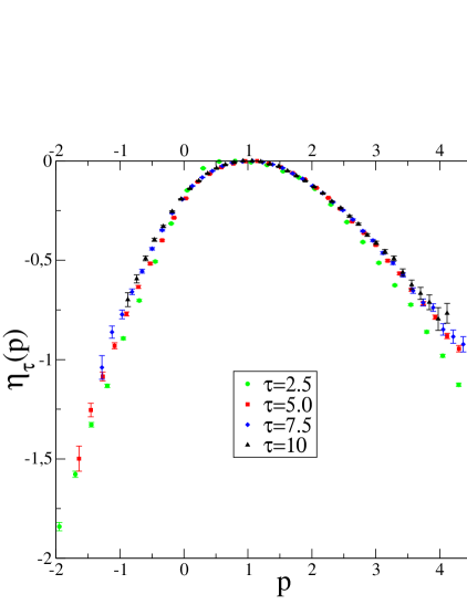
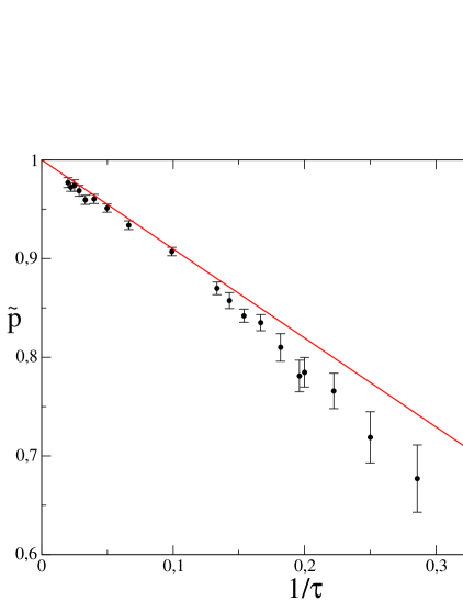
Figure 5.1: Model I at $E=5$: (left) the function $\eta_{\tau}(p)=\zeta_{\infty}(p)+O((p-1)^{2}/\tau)$ for different values of $\tau$; (right) the maximum $\widetilde{p}_{\tau}$ of $\zeta_{\tau}(p)$ as a function of $1/\tau$. The full line is the prediction of Eq. (5.16), $\widetilde{p}=1-\zeta_{\infty}^{(3)}/\big{[}2\tau\big{(}\zeta_{\infty}^{(2)}\big{)}^{2}\big{]}$.

In this section the procedure followed to analyze the numerical data will be described in detail. As an example, the data obtained from the simulation of model I at $E=5$ will be discussed. From the simulation run a set ${\cal P}_{0}=\{p_{i}\}_{i=1\ldots{\cal N}}$ of values of the variable $p(x)$ is obtained, that correspond to $\tau=\tau_{0}$ and are measured on adjacent segments of trajectory. As discussed above, $\tau_{0}=0.1=100dt$ is of the order of the mixing time, i.e. the time scale over which the correlation functions (e.g. of density fluctuations) decay to zero.

Probability distribution function

From the dataset ${\cal P}_{0}$ the histograms $\pi_{\tau}(p)$ are constructed for different values of $\tau=n\tau_{0}$ as follows: the values of $p(x)$ for $\tau=n\tau_{0}$ are obtained by averaging $n$ subsequent entries of the dataset ${\cal P}_{0}$; one obtains a new dataset ${\cal P}_{n}=\{p^{(n)}_{j}\}_{j=1\ldots{\cal N}/n}$ such that $p^{(n)}_{j}=n^{-1}\sum_{i=nj+1}^{n(j+1)}p_{i}$. Finally, from the dataset ${\cal P}_{n}$ the histogram of $\pi_{\tau}(p)$ is constructed for $\tau=n\tau_{0}$; the errors are estimated as the square roots of the number of counts in each bin. The function $\zeta_{\tau}(p)$ is then defined as $\zeta_{\tau}(p)=\tau^{-1}\log\pi_{\tau}(p)$.

Shifting of the maximum

By fitting the function $\zeta_{\tau}(p)$ in $p\in[-1,3]$ with a sixth-order polynomial the position of the maximum $\widetilde{p}_{\tau}$ is determined within an error that, since $\delta p$ is the length of a bin, is estimated to be $\delta p/2$. Then, the function $\eta_{\tau}(p)=\zeta_{\tau}(p-1+\widetilde{p}_{\tau})$ is constructed, see Eq. (5.18); it is expected to approximate the limiting function $\zeta_{\infty}(p)$ with error $O((p-1)^{2}/\tau)$. The functions $\eta_{\tau}(p)$ are reported in Fig. 5.1 for different values of $\tau$. A very good convergence for $\tau\gtrsim 5.0=50\tau_{0}$ is observed.

By a fourth-order fit of the so-obtained limiting function $\zeta_{\infty}(p)$ around $p=1$ the coefficients $\zeta_{\infty}^{(2)}=-0.287$ and $\zeta_{\infty}^{(3)}=0.149$ are extracted in order to test the correctness of Eq. (5.16). In Fig. 5.1 $\widetilde{p}_{\tau}$ is reported. The full line is the prediction of Eq. (5.16), that is indeed verified for $\tau\gtrsim 10$. This result confirms the analysis of section 5.2.

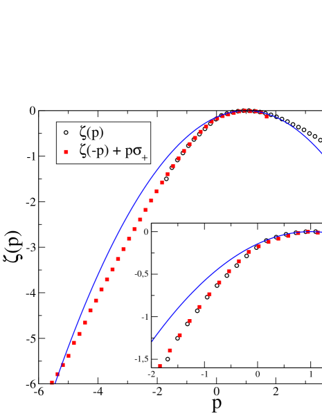
Figure 5.2: Model I at $E=5$: the estimate of the function $\zeta_{\infty}(p)$ (open circles). In the same plot $\zeta_{\infty}(-p)+p\sigma_{+}$ (filled squares) is reported. In the inset, the interval $p\in[-2,2]$ where the data overlap is magnified. The full line is the Gaussian approximation, $\frac{1}{2}\zeta_{\infty}^{(2)}(p-1)^{2}$. The plot shows that the Gaussian is not a good approximation in the interval $[-2,2]$. The validity of the Fluctuation Relation in the same interval is shown by the overlap of the open circles and filled squares.

Graphical verification of the fluctuation relation

From the previous analysis one can conclude that the function $\eta_{\tau}(p)$ for $\tau=5.0$ provides a good estimate of the function $\zeta_{\infty}(p)$ for $p\in[-2,4]$ (see Fig. 5.1); thus, one can use this function to test the fluctuation relation, Eq. (4.11), in this range of $p$. In Fig. 5.2 the estimated functions $\zeta_{\infty}(p)$ and $\zeta_{\infty}(-p)+p\sigma_{+}$ are reported. An excellent agreement between the two functions is observed in the interval $p\in[-2,2]$ where the data allows the computation of both $\zeta_{\infty}(p)$ and $\zeta_{\infty}(-p)$. Note that in this range of $p$ the function $\zeta_{\infty}(p)$ is not Gaussian, see the inset of Fig. 5.2.

Quantitative verification of the fluctuation relation

The translation of the function $\zeta_{\tau}(p)$ is crucial to obtain a correct estimate of the limit $\zeta_{\infty}(p)$ and to verify the fluctuation relation. In this section an attempt to quantify this observation is presented; as the discussion will be very technical, the reader who is satisfied with Fig. 5.2 should skip to next section.

The histogram $\pi_{n\tau_{0}}(p)$ derived from the dataset ${\cal P}_{n}$ is constructed assigning the number of counts $\pi_{\alpha}$ in the $\alpha$-th bin to the middle of the binning interval, that will be called $p_{\alpha}$ (the latter will be an increasing function of $\alpha$). The statistical error $\delta\pi_{\alpha}$ on the number of counts is $\sqrt{\pi_{\alpha}}$. The histograms are constructed in such a way that if $p_{\alpha}$ is the center of a bin, also $-p_{\alpha}$ is the center of a bin; $\overline{\alpha}$ is the bin such that $p_{\overline{\alpha}}=-p_{\alpha}$. There exists a value $p_{m}$ such that for $p_{\alpha}<p_{m}$ the number of counts in the bin $\alpha$ is smaller than $m$ ($m=4$ has been chosen in the present analysis). Define $p_{\alpha_{m}}$ the smallest value of $p_{\alpha}>p_{m}$. Hence, the histogram is characterized by:

1. a bin size $\delta p$;

2. the bin $\alpha_{m}$ corresponding to the minimum value of $p_{\alpha}$ such that the number of counts in the bin is at least $m$;

3. the total number $M$ of bins such that $\alpha\in[\alpha_{m},\overline{\alpha}_{m}]$; for these values of $p_{\alpha}$, both $\pi_{\tau}(p)$ and $\pi_{\tau}(-p)$ can be computed and they can be used to verify the fluctuation relation.

The function $\zeta_{\tau}(p)$, derived from the histogram, is specified by a set of values $(p_{\alpha},\zeta_{\alpha},\delta\zeta_{\alpha})$ for each bin $\alpha$, where $\zeta_{\alpha}=\tau^{-1}\log\pi_{\alpha}$ and the error $\delta\zeta_{\alpha}$ has been defined by

$$\delta\zeta_{\alpha}=\frac{1}{\tau}\frac{\delta\pi_{\alpha}}{\pi_{\alpha}}=\frac{1}{\tau\sqrt{\pi_{\alpha}}}\ .$$ (5.30)

A quantitative verification of Eq. (4.11) is possible defining the following $\chi^{2}$ function:

$$\chi^{2}\equiv\frac{1}{M}\sum_{\alpha=\alpha_{m}}^{\overline{\alpha}_{m}}\frac{(\zeta_{\alpha}-\zeta_{\overline{\alpha}}-p_{\alpha}\sigma_{+})^{2}}{(\delta\zeta_{\alpha})^{2}+(\delta\zeta_{\overline{\alpha}})^{2}}\ .$$ (5.31)

The value of $\chi$ is the average difference between $\zeta_{\tau}(p)$ and $\zeta_{\tau}(-p)+p\sigma_{+}$ in units of the statistical error. Translating $p$ of a quantity $a\delta p/2$, $a\in\hbox{\msytw Z}$, corresponds to shifting the histogram, i.e. to consider a new histogram $(p_{\alpha}+a\delta p/2,\zeta_{\alpha},\delta\zeta_{\alpha})$. This preserves the property that if $p_{\alpha}$ is the center of a bin, also $-p_{\alpha}$ is the center of a bin; let $\overline{\alpha}(a)$ be the new value of $\alpha$ such that $p_{\overline{\alpha}(a)}+a\delta p/2=-(p_{\alpha}+a\delta p/2)$. Also, the number $M_{a}$ of bins such that $\alpha(a)\in[\alpha_{m},\overline{\alpha}_{m}(a)]$ depends on $a$. Define

$$\chi^{2}(a)\equiv\frac{1}{M_{a}}\sum_{\alpha=\alpha_{m}}^{\overline{\alpha}_{m}(a)}\frac{\big{(}\zeta_{\alpha}-\zeta_{\overline{\alpha}(a)}-(p_{\alpha}+a\delta p/2)\sigma_{+}\big{)}^{2}}{(\delta\zeta_{\alpha})^{2}+(\delta\zeta_{\overline{\alpha}(a)})^{2}}\ .$$ (5.32)

The criterion that will be followed is that the fluctuation relation is satisfied if $\chi\leq 3$, which means that $\zeta_{\infty}(p)$ and $\zeta_{\infty}(-p)+p\sigma_{+}$ differ, on average, by less than $3$ times the statistical error $\sqrt{\big{(}\delta\zeta(p)\big{)}^{2}+\big{(}\delta\zeta(-p)\big{)}^{2}}$. The function $\chi(a)$ for the case of model I at $E=5$ is reported in Fig. 5.3.

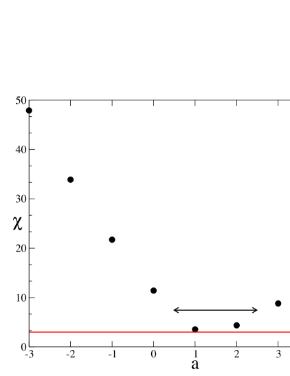
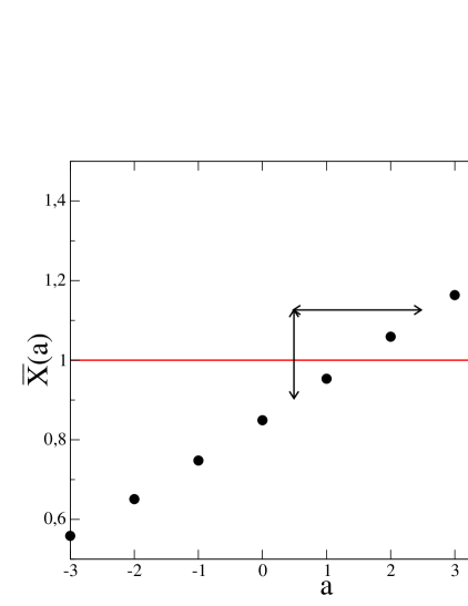
Figure 5.3: Model I at $E=5$: (left) the function $\chi(a)$. The full line corresponds to $\chi=3$. The arrow indicates the interval $\delta_{0}\pm\delta p/2$ (note that its length is 2 in units of $a$) into which the minimum of $\chi$ can be located within the accuracy of the histogram. (right) The function $\overline{X}(a)$. The horizontal arrow marks the interval where the minimum of $\chi$ is located, see the left panel. The vertical arrow indicates the error $\delta X$ on the value $X=1$ which is estimated as $\delta X=2(\overline{X}(2)-\overline{X}(1))$. The slope of the fluctuation relation without the translation would have been $\overline{X}(a=0)\sim 0.85$.

The minimum of $\chi$ is assumed between $a^{*}=1$ and $a^{*}+1=2$ and an upper limit for the value of $\chi$ at the minimum is $\chi(1)=3.5$. The translation that minimizes $\chi$ is estimated as $\delta_{0}=(a^{*}+0.5)\delta p/2=1.5\cdot 0.093=0.140$, and to this estimate an error $\pm\delta p/2$ is attributed, where $\delta p=0.186$ is the size of a bin. On the other hand, as discussed above, in order to shift the maximum of $\zeta_{\tau}(p)$ in $p=1$, one has to translate $p$ by a quantity $\delta\equiv 1-\widetilde{p}=0.215$. The consistency of the analysis requires that $\delta$ and $\delta_{0}$ coincide within their errors, i.e. that the intervals $\delta\pm\delta p/2$ and $\delta_{0}\pm\delta p/2$ overlap, or in other words $|\delta-\delta_{0}|<\delta p$. In the present case $0.075=|\delta-\delta_{0}|<\delta p=0.186$, then $\delta$ and $\delta_{0}$ coincide within the errors. This means that the translation of $p$ brings the maximum of $\zeta_{\tau}(p)$ in $p=1$ and, at the same time, minimizes the difference between $\eta_{\tau}(p)$ and $\eta_{\tau}(-p)+p\sigma_{+}$, where $\eta_{\tau}$ is the finite time estimate of $\zeta_{\infty}(p)$. The value $\chi(a^{*})$ quantifies this difference and is a first estimate of the precision of the analysis.

Another estimate of the precision of the analysis can be obtained as follows. Define a parameter $X$ as the slope of $\zeta_{\infty}(p)-\zeta_{\infty}(-p)$ as a function of $p\sigma_{+}$:

$$\zeta_{\infty}(p)=\zeta_{\infty}(-p)+Xp\sigma_{+}\ .$$ (5.33)

The fluctuation theorem predicts $X=1$, but other values of $X$ are possible under different hypothesis, see [84, 95, 112, 129]. Defining a function $\chi^{2}(a,X)$ as

$$\chi^{2}(a,X)\equiv\frac{1}{M_{a}}\sum_{\alpha=\alpha_{m}}^{\overline{\alpha}_{m}(a)}\frac{\big{(}\zeta_{\alpha}-\zeta_{\overline{\alpha}(a)}-X(p_{\alpha}+a\delta p/2)\sigma_{+}\big{)}^{2}}{(\delta\zeta_{\alpha})^{2}+(\delta\zeta_{\overline{\alpha}(a)})^{2}}\ ,$$ (5.34)

for each value of $a$ one can calculate the optimal value of $X$, $\overline{X}(a)$, by minimizing $\chi^{2}(a,X)$. The function $\overline{X}(a)$ is reported in Fig. 5.3. As the shift of the maximum $\delta$ is between $a=1$ and $a=2$, the slope $X$ is compatible with one. Moreover, as the natural error on $p$ is the size of a bin $\delta p$, it is reasonable to assign to the value $X=1$ a statistical error $\delta X=2(\overline{X}(2)-\overline{X}(1))=0.22$. Note again that without the translation of $p$ the optimal slope would be $X\sim 0.85$, incompatible with Eq. (4.11).

Discussion

From the present analysis, one can conclude that:

1. the translation shifting the maximum of $\zeta_{\tau}(p)$ to $p=1$ at the same time minimizes the difference between $\eta_{\tau}(p)$ and $\eta_{\tau}(-p)+p\sigma_{+}$, where $\eta_{\tau}$ is the finite time estimate of $\zeta_{\infty}$; this proves the consistency of the theory of finite time corrections described above;

2. without the translation of $p$ (that corresponds to $a=0$), the function $\zeta_{\tau}(p)$ for $\tau\sim 5.0$ does not satisfy the fluctuation relation, as $\chi(a=0)=11$ and $\overline{X}(a=0)=0.85$;

3. the function $\eta_{\tau}(p)=\zeta_{\tau}(p-\delta)$ satisfies the fluctuation relation with $\chi\sim 3$ and an error of about $20\%$ on the slope $X$: both quantities measure the accuracy of the data analysis.

Thus, the check of the fluctuation relation relies crucially on the translation of the function $\zeta_{\tau}(p)$ that has been discussed in section 5.2. By considering larger values of $\tau$ one could avoid this problem (as $\delta\sim\tau^{-1}$); however, as one can see from Fig. 5.1, for $\tau>5.0$ the negative tails of $\zeta_{\tau}(p)$ are not accessible to the computational resources available during this work. The computation of the finite time corrections is mandatory if one aims to test the fluctuation relation at high values of the external driving force.

Summary of the data analysis

To summarize, the procedure followed to analyze the data of a given simulation run is:

1. a value of $\tau$ such that $\zeta_{\tau}(p)$ appear to be close to the asymptotic limit $\zeta_{\infty}(p)$ is determined;

2. the maximum $\widetilde{p}$ of $\zeta_{\tau}(p)$ is obtained by a sixth-order polynomial fit around $p=1$, in an interval as big as possible compatibly with the request that the $\chi^{2}$ from the fit is less than $\sim 10$;

3. the histogram is shifted by an integer multiple $a$ of the half bin size $\delta p/2$ and the function $\chi(a)$ is computed according to Eq. (5.32). The value $a^{*}$ such that the minimum of $\chi(a)$ is assumed in the interval $[a^{*},a^{*}+1]$ is determined: the consistency of the analysis requires that $\delta=1-\widetilde{p}$ and $\delta_{0}=(a^{*}+0.5)\delta p/2$ coincide within their errors (i.e. $|\delta-\delta_{0}|<\delta p$);

4. The value $\chi^{*}=\min[\chi(a^{*}),\chi(a^{*}+1)]$ is an upper limit for the value of $\chi$ at the minimum. The number of bins $\min\{M_{a^{*}},M_{a^{*}+1}\}$ involved in this estimate will be called $M^{*}$;

5. the error $\delta X=2(\overline{X}(a^{*}+1)-\overline{X}(a^{*}))$ is computed.

The relevant quantities $\tau$, $\delta$, $\delta_{0}$, $|\delta-\delta_{0}|$, $\delta p$, $M^{*}$, $\chi^{*}$ and $\delta X$ for model I are reported in table 5.1 for different values of the external force $E$.

5.5 Numerical simulation of model I

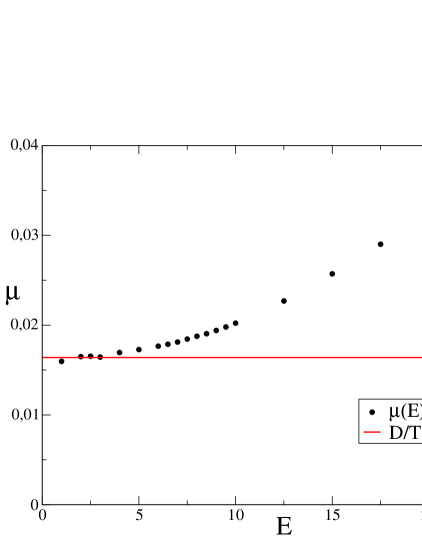
Figure 5.4: Model I: mobility $\mu$ as a function of the driving force $E$. The full line is the equilibrium diffusion coefficient $D$ divided by the temperature. Deviations from the linear response are observed around $E=5$. The error bars are of the order of the dimension of the symbols. Studying $\mu(E)$ for values of $E$ bigger than those shown in the figure, one can verify that the mobility increases up to a value $\mu_{max}$, reached in correspondence of $E\sim 45$. For values of $E$ bigger than $E\sim 45$, the mobility begins to decrease essentially following the limiting curve $T{\cal J}_{T}/(NE)$, where ${\cal J}_{T}=\sqrt{T(d-1/N)}N/T$ is the maximum allowed value of the current (saturation value).

$E$	$\tau$	$\sigma_{+}$	$\delta$	$\delta_{0}$	$|\delta-\delta_{0}|$	$\delta p$	$M^{*}$	$\chi^{*}$	$\delta X$
2.5	5.0	0.194	0.272	0.183	0.089	0.244	43	2.2	0.24
5.0	5.0	0.810	0.215	0.139	0.076	0.187	20	3.5	0.22
7.5	4.0	1.945	0.197	0.116	0.081	0.116	18	2.8	0.18
10.0	2.5	4.044	0.262	0.151	0.111	0.122	17	4.4	0.20
12.5	2.5	7.090	0.257	0.137	0.120	0.111	8	3.5	0.28

Table 5.1: Model I: results of the data analysis for some selected values of $E$. All the quantities are defined in section 5.4. For $E>12.5$ the negative tails of the distribution are not accessible to the numerical simulation.

The numerical data obtained from the simulation of model I (defined in section 5.3) will now be discussed systematically at different values of the driving force $E$. In Fig. 5.4 the mobility $\mu(E)=T\langle{\cal J}\rangle_{E}/(NE)$, i.e. the l.h.s. of Eq. (4.38) times $T/N$, is reported as a function of $E$. The current ${\cal J}({\underline{p}},{\underline{q}})$ has been defined in Eq. (5.24). From the Green-Kubo relation, Eq. (4.36), one has [80]

$$\lim_{E\rightarrow 0}\mu(E)=\frac{D}{T}\ ,$$ (5.35)

where $D$ is the equilibrium diffusion coefficient,

$$D=\lim_{t\rightarrow\infty}\frac{1}{2Nd}\sum_{i}\langle|q_{i}(t)-q_{i}(0)|^{2}\rangle_{E=0}\ .$$ (5.36)

Deviations from the linear response are observed and $\mu(E)\sim D/T+O(E^{2})$ above $E=5$.

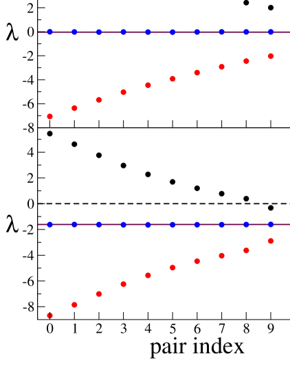
Figure 5.5: Model I: Lyapunov exponents for $E=5$ (top) and for $E=25$ (bottom). For each panel, the upper and lower dots are the two paired exponents $\lambda^{(+)}_{j}$ and $\lambda^{(-)}_{j}$, and the middle dot is their average $(\lambda^{(+)}_{j}+\lambda^{(-)}_{j})/2$. The full line is $\sigma_{+}/2Nd$, the dashed line is at $\lambda=0$.

In table 5.1 the main parameters that result from the data analysis (as discussed in the previous section) are reported for some selected values of $E$. The value $|\delta-\delta_{0}|$ is always less than $\delta p$, consistently with the discussion above, except for $E=12.5$ where, however, the relative difference between the two quantities is small ($\sim 9\%$). It can be noted that $\delta$ is systematically bigger than $\delta_{0}$. This could be due to the fact that the error terms $O((p-1)^{2}/\tau)$ or $o(1/\tau)$ that have been discarded likely produce a systematic shift in $\delta$ or in $\delta_{0}$; or that the velocity of convergence of $\zeta_{\tau}(p)$ is not the same on the negative or on the positive side (because numerically is much more difficult to observe big negative fluctuations of $\sigma$ than the positive ones – and the Fluctuation Relation provides a quantitative estimate of the relative probabilities). At the moment, because of the level of precision of the simulations, it is not possible to investigate this problem in more detail, see also Remark (3) in section 5.2.3. On increasing the value of $E$, one is forced to decrease the value of $\tau$ used for the analysis as, for longer $\tau$, the negative tail of the distribution $\zeta_{\tau}(p)$ becomes unobservable. This can be seen as the number $M^{*}$ of bins used for the computation of $\chi$ decrease on increasing $E$; above $E=12.5$ it is impossible to find a value of $\tau$ such that $\zeta_{\tau}(p)$ is close to the asymptotic limit and the negative tail is observable. Thus, the fluctuation relation cannot be tested above $E=12.5$ with the present computational power. However, the fluctuation relation has been checked in the region $E>5$ where deviations from the linear response are observed. Moreover, the estimated distributions $\zeta_{\infty}(p)$ are very similar to the one reported in Fig. 5.2: in particular, they are not Gaussian in the investigated interval of $p$ (also for $E<5$, in the linear response regime).

Finally, in Fig. 5.5 the measured Lyapunov exponents of the model for $E=5$ and $E=25$ are reported. For this system, the Lyapunov exponents are known to be paired [125, 130, 131] like in Hamiltonian systems and the average of each pair is a constant equal to $\sigma_{+}/2Nd$. For $E=5$, each pair is composed of a negative and a positive exponent. This means that the attractive set is dense in phase space [95, 112] and the chaotic hypothesis is expected to apply to the system yielding a slope $X=1$ in the fluctuation relation, as confirmed by the numerical data. The same happens up to $E\sim 20$. Above $E=20$, there is a number $D$ of pairs composed by two negative exponents (for $E=25$ one has $D=4$, see Fig. 5.5). In this situation, the slope $X$ in the fluctuation relation is expected to be given by $X=1-D/Nd$ [112, 129]. Thus, for $E=25$ one expects $X\sim 0.75$. Unfortunately, as discussed above, above $E=12.5$ negative fluctuations of the entropy production are not observed, and this prediction could not be tested in the present simulation.

5.6 Numerical simulation of model II

Figure 5.6: Mobility as a function of the temperature $T$ and of the driving force $E$ for Model II. The circles correspond to the equilibrium diffusion coefficient divided by the temperature. Deviations from the linear response are observed for $E\geq 3$; they become larger on lowering the temperature, as $D\rightarrow 0$.

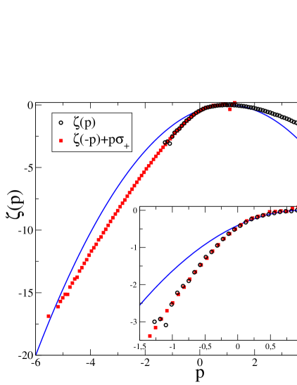
Figure 5.7: The estimate of the function $\zeta_{\infty}(p)$ (open circles) for Model II with $T=1.1$ and $E=3$. In the same plot $\zeta_{\infty}(-p)+p\sigma_{+}$ (filled squares) is reported. In the inset, the interval $p\in[-1.5,1.5]$ where the data overlap is magnified. The full line is the Gaussian approximation, $\zeta_{\infty}(p)=\frac{1}{2}\zeta_{\infty}^{(2)}(p-1)^{2}$. The data have been obtained from the histogram of $\pi_{\tau}(p)$ with $\tau=2.5$ (see table 5.2).

$T$	$E$	$\tau$	$\sigma_{+}$	$\delta$	$\delta_{0}$	$|\delta-\delta_{0}|$	$\delta p$	$M^{*}$	$\chi^{*}$	$\delta X$
0.9	1	3.0	0.209	0.453	0.334	0.119	0.223	68	1.9	0.19
0.9	3	3.0	2.615	0.286	0.264	0.024	0.132	15	1.0	0.23
1.1	1	4.0	0.233	0.231	0.126	0.105	0.126	79	1.7	0.24
1.1	3	2.5	2.493	0.217	0.238	0.021	0.087	30	1.0	0.12
1.1	6	1.5	13.32	0.113	0.230	0.117	0.092	7	1.1	0.21
1.5	1	3.0	0.230	0.179	0.140	0.039	0.140	86	0.9	0.13
1.5	3	2.5	2.227	0.145	0.123	0.022	0.082	33	4.7	0.18
1.5	6	0.5	52.14	0.074	0.130	0.056	0.052	11	0.6	0.10
1.7	1	3.0	0.221	0.127	0.141	0.014	0.283	49	1.0	0.26
1.9	3	2.5	1.981	0.106	0.122	0.016	0.122	26	0.8	0.12
1.9	6	0.4	43.52	0.078	0.126	0.048	0.085	14	1.7	0.11
1.9	10	0.2	139.0	0.079	0.135	0.056	0.039	7	0.8	0.10
2.1	6	0.4	40.48	0.074	0.110	0.036	0.110	11	1.0	0.15

Table 5.2: Model II: results of the data analysis for some selected values of $T$ and $E$. All the quantities are defined in section 5.4.

Model II differs from model I in the dimension $d=3$, in the larger number of particles $N=20$, and because it is a binary mixture of two types of particles. Binary mixtures are frequently used as models for numerical simulations of supercooled liquids as they avoid crystallization also at very low temperature on the ”physical” time scales (i.e. on the time scales of numerical experiments); for these systems, at low temperature deviations from the linear response are observed also for very low values of the external driving force.

In Fig. 5.6 the equilibrium diffusion coefficient $D$ (divided by the temperature $T$) and the mobility (for different values of $E$) are reported as functions of the temperature. Even though the number of particles is very small, on lowering the temperature the systems approaches the supercooled state and $D$ becomes very small around $T\sim 0.5$. Slightly above this temperature, i.e. around $T=1$, strong deviations from the linear response are observed for $E\geq 3$, where the entropy production $\sigma_{+}$ is still close to $0$. Some values of $\sigma_{+}$ are reported in table 5.2; to compare these values with those obtained for model I one should note that $\sigma_{+}$ is an extensive quantity. Thus, the entropy production per degree of freedom, $\sigma_{+}/2Nd$, is much smaller in model II than in model I.

In table 5.2 the results of the data analysis outlined in section 5.4 are reported. For $E\leq 6$ a very good agreement of the data with the predictions of the fluctuation relation and with the theory of finite time corrections discussed in section 5.2 is obtained. For $E=10$ it is very difficult to observe negative fluctuations of $p$ with the available computational power; see e.g. the result of the analysis for $E=10$ and $T=1.9$, where only $M^{*}=7$ bins where available and it was mandatory to use $\tau=0.2$, of the order of the mixing time $\tau_{0}$. In Fig. 5.7 the estimated function $\zeta_{\infty}(p)$ obtained for $T=1.1$ and $E=3$ from the data with $\tau=2.5$ is reported. Strong deviations from the Gaussian behavior are observed in the accessible range of $p$ (see the inset of Fig. 5.7). A similar behavior of $\zeta_{\infty}(p)$ is observed in correspondence of all the values of $E$ and $T$ that were investigated (those listed in Table II): in particular in all these cases highly non Gaussian behaviors are observed in the accessible range of $p$.

The Lyapunov spectrum for this system is very similar to the one reported in the upper panel of Fig 5.5. Pairs of two negative exponents were observed only for $E=10$ at $T\leq 1.3$, where, as in the case of Model I, $\sigma_{+}$ is too large to allow for a verification of the modified fluctuation relation expected in this case, see the discussion at the end of section 5.5.

5.7 Discussion

The fluctuation relation has been tested, quite successfully, in a numerical simulation of two models of interacting particles subjected to an external nonconservative force and to a reversible mechanical thermostat. The data satisfy the fluctuation relation with a $\chi\leq 3$ and an accuracy of the order of $20\%$ also for very large values of the driving force, where strong deviations from the linear response are observed, and where the large deviation function is strongly non-Gaussian. The comparison of the numerical data with the predictions of the fluctuation relation is done by taking into account the (lowest order) finite time corrections to the distribution function for the fluctuations of the phase space contraction rate. This is crucial: if such corrections were not taken into account, the fluctuation relation would be violated within the precision of the experiment.

In order to compute the finite time corrections, an algorithm which allows to reconstruct the asymptotic distribution function from measurable quantities at finite time, within a given precision, has been proposed. The theory of the corrections relies on the symbolic representation of the chaotic dynamics, therefore it is applicable if one accepts the Chaotic Hypothesis.

The numerical results support the conjecture that the chaotic hypothesis can be applied to these systems, also very far from equilibrium, and in particular the fluctuation relation is satisfied even in regions where its predictions measurably differ from those of linear response theory.

The theory of finite time corrections for the analysis of the numerical data could in principle be of interest for real experimental settings where non Gaussian fluctuations for the entropy production rate are observed, see e.g.  [103, 106].

However it should be stressed that in a real experiment there are some technical differences with respect to the numerical simulation which could in some cases make inapplicable the analysis, namely:
(i) usually the noise in the large deviation function for the entropy production rate in a real experiment is much bigger than in a numerical experiment, and it is likely that the translation in Eq. (5.18) computed as the ratio $\zeta^{(3)}/(\zeta^{(2)})^{2}$ is not measurable within an error of some percent;
(ii) usually in a real experiment the accessible time scales are naturally much bigger than the microscopic ones so that, if the negative fluctuations of the entropy production rate are observable at all, one is automatically in the asymptotic regime, where the finite time corrections should be negligible;
(iii) a usual problem in a realistic setting is that there is no clear connection between the “natural” thermodynamic entropy production rate $\dot{s}=W/T$ ($W$ is the work of the dissipative external forces and $T$ is the temperature) and the microscopic phase space contraction rate, for which a slope $X=1$ in the fluctuation relation $\zeta(p)-\zeta(-p)=X\sigma_{+}p$ is expected; so, often one measures an $X\neq 1$ and correspondingly one defines an effective temperature $\Theta_{eff}=T/X$ giving a natural connection between the effective thermodynamic entropy production rate $\dot{s}_{eff}=W/\Theta_{eff}$ and the phase space contraction rate, see [84, 103, 106] and the following chapters; in such a situation (where an adjustable parameter $X$ appears) it makes no sense to apply this analysis, which is sensible only if one wants to compare the experimental data with a sharp prediction about the slope $X$ in the fluctuation relation.

A big problem which is left open is trying to understand how the fluctuation relation is modified for values of the driving force so high that the attractive set is no longer dense in phase space. It is expected, [129], that in such a case $\zeta_{\infty}(p)-\zeta_{\infty}(-p)$ is still linear, but the slope is $X\sigma_{+}$, with $X$ given by the ratio of the dimension of the attractive set and of that of the whole phase space. An estimate of such quantity can be given via the number of negative pairs of exponents in the Lyapunov spectrum [112, 129]. Unfortunately negative pairs begin to appear in the Lyapunov spectrum only for values of the external force so high that no negative fluctuations are observable anymore. Hopefully future work will address this point.

5.8 Appendix: A Limit Theorem

In this section Eq.s (5.9–5.10) will be proved. The proof is presented in the case $p$ is the average of independently distributed discrete variables $\sigma_{i}^{\varepsilon}$, assuming values in $\varepsilon\hbox{\msytw Z}$, for some small mesh parameter $\varepsilon$; then how this can be applied and adapted to the situation considered in section 5.2 and subsequent sections will be discussed.

Let $\sigma_{i}$, $i\in\hbox{\msytw N}$, be independent continuous random variables with identical distributions $\pi(d\sigma_{i})$ with positive variance $\delta\sigma^{2}>0$, supported on the finite interval $[s_{-},s_{+}]$. Assume that $\pi(d\sigma_{i})$ gives positive probability to any finite interval contained in $[s_{-},s_{+}]$. Let $\pi_{\lambda}(d\sigma)$ be the weighted distribution $\pi_{\lambda}(d\sigma)=e^{-\lambda\sigma}\pi(d\sigma)/\int e^{-\lambda\sigma}\pi(d\sigma)$ and define $z_{\infty}(\lambda)=-\log\int e^{-\lambda\sigma}\pi(d\sigma)$ and $\sigma_{+}=z_{\infty}^{\prime}(0)$. Note that the assumption that $\pi(d\sigma_{i})$ gives positive probability to an interval of $\sigma$ in $[s_{-},s_{+}]$ implies that for any finite $\lambda$ also $\pi_{\lambda}(d\sigma)$ has positive variance $-z_{\infty}^{\prime\prime}(\lambda)>0$.

Also, given $\varepsilon>0$ (with the property that $s_{+}-s_{-}=N_{\varepsilon}\varepsilon$ for some integer $N_{\varepsilon}$), consider the discretization of $\sigma_{i}$ on scale $\varepsilon$, and call it $\sigma_{i}^{\varepsilon}$: $\sigma_{i}^{\varepsilon}$ will be a discrete variable assuming the values $s_{k}^{\varepsilon}\equiv s_{-}+(k-\frac{1}{2})\varepsilon$, $k=1,\ldots,N_{\varepsilon}$, with probabilities $\pi^{\varepsilon}(s_{k}^{\varepsilon})={\rm Prob}(\sigma_{i}^{\varepsilon}=s_{k}^{\varepsilon})=\int_{s_{k}^{\varepsilon}\pm\frac{\varepsilon}{2}}\pi(d\sigma)$. The assumption that $\pi(d\sigma_{i})$ gives positive probability to any finite interval contained in $[s_{-},s_{+}]$ implies that $\pi^{\varepsilon}(s_{k}^{\varepsilon})>0$ for any $\varepsilon$ and $k$. Let also $z_{\varepsilon}(\lambda)=-\log\sum_{k=1}^{N_{\varepsilon}}e^{-\lambda s_{k}^{\varepsilon}}\pi^{\varepsilon}(s_{k}^{\varepsilon})$ and $\pi^{\varepsilon}_{\lambda}(s_{k}^{\varepsilon})=\pi^{\varepsilon}(s_{k}^{\varepsilon})e^{-\lambda s_{k}^{\varepsilon}+z_{\varepsilon}(\lambda)}$. Note that, since $\pi^{\varepsilon}(s_{k}^{\varepsilon})>0$ for any $k$, for any finite $\lambda$ one has $-z_{\varepsilon}^{\prime\prime}(\lambda)>0$.

If $p_{\tau}^{\varepsilon}=\frac{1}{\tau\sigma_{+}}\sum_{i=1}^{\tau}\sigma_{i}^{\varepsilon}$ and $\Pi_{\tau}(\varepsilon;I)$ is the probability that $p_{\tau}^{\varepsilon}$ belongs to the finite interval $I$, the following theorem holds.

Theorem: Given a finite interval $I\subset(s_{-},s_{+})$, let $\sigma_{i}^{\varepsilon}$, $\pi^{\varepsilon}$ and $\Pi_{\tau}(\varepsilon;I)$ be defined as above. Then, for a sufficiently small $\varepsilon>0$, there exists an analytic ”rate function” $\widetilde{\zeta}_{\tau}(p)$ such that

$$\lim_{\tau\rightarrow\infty}\frac{\Pi_{\tau}(\varepsilon;I)}{\int_{I}dpe^{\tau\widetilde{\zeta}_{\tau}(p)}}=1\;.$$ (5.37)

$\widetilde{\zeta}_{\tau}(p)$ is defined by:

$$\begin{split}&\widetilde{\zeta}_{\tau}(p)+\frac{1}{\tau}\log\Big{[}\frac{\sinh[\varepsilon\lambda_{p}^{\varepsilon}/(2\sigma_{+})]}{\varepsilon\lambda_{p}^{\varepsilon}/(2\sigma_{+})}\Big{]}=\zeta_{\tau}^{\varepsilon}(p)\\ &\zeta_{\tau}^{\varepsilon}(p)=-z_{\varepsilon}(\lambda_{p}^{\varepsilon})+\lambda_{p}^{\varepsilon}p\sigma_{+}-\frac{1}{2\tau}\log[\frac{2\pi}{\tau}\Big{(}-\frac{z_{\varepsilon}^{\prime\prime}(\lambda_{p}^{\varepsilon})}{\sigma_{+}^{2}}\Big{)}]\end{split}$$ (5.38)

and $\lambda_{p}^{\varepsilon}$ is the inverse of $p(\lambda)=z_{\varepsilon}^{\prime}(\lambda)/\sigma_{+}$. The function $\zeta_{\tau}^{\varepsilon}(p)$ has the following property: if $\Delta\subset I$ is an interval of size $\frac{\varepsilon}{\tau\sigma_{+}}$ around a point $p_{\Delta}$, then:

$$\lim_{\tau\rightarrow\infty}\frac{\Pi_{\tau}(\varepsilon;\Delta)}{|\Delta|e^{\tau\zeta_{\tau}^{\varepsilon}(p_{\Delta})}}=1$$ (5.39)

Proof Define the auxiliary variable $q=\frac{1}{\tau\sigma_{+}}\sum_{i=1}^{\tau}\eta_{i}$, where $\eta_{i}$ are i.i.d. discrete random variables, with distribution $\pi_{\lambda}^{\varepsilon}(s_{k}^{\varepsilon})$. Let $\Pi_{\tau}^{\lambda}(\varepsilon;q_{0})$ be the probability that $q$ assumes the value $q_{0}\in I$, with $q_{0}\sigma_{+}=s_{k}^{\varepsilon}/\tau$ for some $k\in\hbox{\msytw N}$, and note that $\Pi_{\tau}^{0}(\varepsilon;q_{0})$ is identical to the probability that $p_{\tau}=q_{0}$. By definition $\Pi_{\tau}^{\lambda}(q_{0})$ and $\Pi_{\tau}^{0}(q_{0})$ are related by:

$$\Pi_{\tau}^{\lambda}(\varepsilon;q_{0})=\frac{e^{-\lambda q_{0}\sigma_{+}\tau}\Pi_{\tau}^{0}(\varepsilon;q_{0})}{\big{[}\sum_{k}e^{-\lambda s_{k}^{\varepsilon}}\pi^{\varepsilon}(s_{k}^{\varepsilon})\big{]}^{\tau}}\ .$$ (5.40)

Now, a local form of central limit theorem (Gnedenko’s theorem, see pag. 211 of [132]) tells that, if $q$ is localized near its mean value, that is if $|q\sigma_{+}-z_{\varepsilon}^{\prime}(\lambda)|\leq\frac{M\varepsilon}{\tau}$ for some finite $M$, then $\Pi_{\tau}^{\lambda}(\varepsilon;q_{0})$ is asymptotically equivalent to the Gaussian with mean $z_{\varepsilon}^{\prime}(\lambda)$ and variance $-z_{\varepsilon}^{\prime\prime}(\lambda)$, in the sense that

$$\Pi_{\tau}^{\lambda}(q_{0})=\frac{\varepsilon}{\sqrt{2\pi\tau(-z_{\varepsilon}^{\prime\prime}(\lambda))}}e^{-\frac{(q_{0}\sigma_{+}-z^{\prime}_{\varepsilon}(\lambda))^{2}}{2(-z_{\varepsilon}^{\prime\prime}(\lambda))}\tau}(1+o(1))\;,$$ (5.41)

for any $q_{0}$ s.t. $|q\sigma_{+}-z_{\varepsilon}^{\prime}(\lambda)|\leq\frac{M\varepsilon}{\tau}$ .

So, given $\lambda_{q_{0}}^{\varepsilon}$ s.t. $z_{\varepsilon}^{\prime}(\lambda_{q_{0}}^{\varepsilon})=q_{0}\sigma_{+}$ (such $\lambda_{q_{0}}^{\varepsilon}$ exists, is unique and is an analytic function of $q_{0}$, by the remark that $-z_{\varepsilon}^{\prime\prime}(\lambda)>0$ for any finite $\lambda$ and $z_{\varepsilon}(\lambda)$ is an analytic function of $\lambda$), using Eq. (5.41), Eq. (5.40) can be restated as:

$$\Pi_{\tau}^{0}(\varepsilon;q_{0})=\frac{\varepsilon}{\sqrt{2\pi\tau(-z_{\varepsilon}^{\prime\prime}(\lambda_{q_{0}}^{\varepsilon}))}}e^{\lambda_{q_{0}}^{\varepsilon}q_{0}\sigma_{+}\tau-z_{\varepsilon}(\lambda_{q_{0}}^{\varepsilon})}(1+o(1))\ .$$ (5.42)

Now, by the definition of $\zeta_{\tau}^{\varepsilon}(p)$ in Eq. (5.38), the r.h.s. of the last equation is equal to $\frac{\varepsilon}{\tau\sigma_{+}}e^{\tau\zeta_{\tau}^{\varepsilon}(q_{0})}(1+o(1))$. Finally, the statement of the Theorem follows by the remark that

$$\frac{\varepsilon}{\tau\sigma_{+}}e^{\tau\zeta_{\tau}^{\varepsilon}(p_{0})}=\int_{p_{0}-\frac{\varepsilon}{2\tau\sigma_{+}}}^{p_{0}+\frac{\varepsilon}{2\tau\sigma_{+}}}dpe^{\tau\tilde{\zeta}_{\tau}(p)}\Big{(}1+o(1)\Big{)}\;.$$ (5.43)

In fact the integral in the r.h.s. of the last equation is given by

$$\begin{split}&e^{\tau\tilde{\zeta}_{\tau}(p_{0})}\int_{p_{0}-\frac{\varepsilon}{2\tau\sigma_{+}}}^{p_{0}+\frac{\varepsilon}{2\tau\sigma_{+}}}dpe^{\tau\tilde{\zeta}_{\tau}^{\prime}(p_{0})(p-p_{0})}\Big{(}1+O(\frac{\widetilde{\zeta}_{\tau}^{\prime\prime}(p_{0})\varepsilon^{2}}{\tau})\Big{)}=\\ &=e^{\tau\tilde{\zeta}_{\tau}(p_{0})}\frac{2\sinh[\tilde{\zeta}_{\tau}^{\prime}(p_{0})\varepsilon/(2\sigma_{+})]}{\tau\tilde{\zeta}_{\tau}^{\prime}(p_{0})}\Big{(}1+O(\frac{\widetilde{\zeta}_{\tau}^{\prime\prime}(p_{0})\varepsilon^{2}}{\tau})\Big{)}\end{split}$$ (5.44)

and in the last expression one has to note that $\widetilde{\zeta}_{\tau}^{\prime}(p_{0})=[\zeta_{\tau}^{\varepsilon}]^{\prime}(p_{0})+O(\frac{1}{\tau})=\lambda_{p_{0}}^{\varepsilon}+O(\frac{1}{\tau}).\$  

A first Remark to be done about the Theorem above is that, in order to define a “universal” rate function in terms of quantities depending only on $z_{\infty}(\lambda)$ (instead of quantities depending on the “non universal” function $z_{\varepsilon}(\lambda)$, which explicitly depends on the discretization step $\varepsilon$), it would desirable to perform (in a sense to be precised) the continuum limit $\varepsilon\rightarrow 0$. To this regard, one can note that the only point where in the proof above the fact that $\varepsilon$ is a constant (i.e. is independent of $\tau$) has been used was in using Gnedenko’s Theorem, see [132]. However, by a critical analysis of the proof of Gnedenko’s Theorem, one can realize that it is even possible to let $\varepsilon=\varepsilon_{\tau}$ go to $0$ with $\tau$; the velocity with which $\varepsilon_{\tau}$ is allowed to go to $0$ depends on the details of the distribution $\pi(d\sigma)$. So one can even study the probability distribution of $p_{\tau}$ on a scale $\sim\varepsilon_{\tau}/\tau$: introducing bins $\Delta_{\tau}$ of size $O(\varepsilon_{\tau}/\tau)$ and defining $\Pi_{\tau}(\Delta_{\tau})$ to be the probability that $p_{\tau}=\frac{1}{\tau\sigma_{+}}\sum_{i}\sigma_{i}$ belongs to the bin $\Delta_{\tau}$ centered in $p_{0}$, one can repeat the proof above to conclude that

$$\lim_{\tau\rightarrow\infty}\frac{\Pi_{\tau}(\Delta_{\tau})}{|\Delta_{\tau}|e^{\tau\zeta_{\tau}(p_{0})}}=1$$ (5.45)

where $\zeta_{\tau}$ satisfies the equation:

$$\zeta_{\tau}(p)=-z_{\infty}(\lambda_{p})+\lambda_{p}p\sigma_{+}-\frac{1}{2\tau}\log[\frac{2\pi}{\tau}\Big{(}-\frac{z_{\infty}^{\prime\prime}(\lambda_{p})}{\sigma_{+}^{2}}\Big{)}]$$ (5.46)

and $\lambda_{p}$ is the inverse of $p(\lambda)=z_{\infty}^{\prime}(\lambda)/\sigma_{+}$.

Another point to be discussed is that in the Theorem above the $\sigma_{i}$ were assumed to be independent. This is not the case for the variables $\sigma(S^{i}\cdot)$ of section 5.2. However, if, as discussed in Remark (3) of section 5.2.3, the time unit is chosen to be of the order of the mixing time, the variables $\sigma(S^{i}\cdot)$ have (by construction) a decorrelation time equal to $1$, and the analysis of previous theorem can be repeated step by step in order to construct the probability distribution of $p=\frac{1}{\tau\sigma_{+}}\sum_{i}\sigma(S^{i}\cdot)$. The only differences are that: (1) $\tau z_{\infty}(\lambda)$ should be replaced by $\tau z_{\tau}(\lambda)=-\log\int e^{-\lambda p\sigma_{+}\tau}\Pi_{\tau}(dp)$ throughout the discussion; (2) instead of Gnedenko’s theorem one has to apply a generalization of Gnedenko’s to short ranged Gibbs processes, to be proven via standard cluster expansion techniques (see for instance [133] for a proof of a generalization of Gnedenko’s theorem to a short ranged Gibbs process in the context of non critical fluctuations of the phase separation line in the 2D Ising model).

The conclusion is that, if the bins $\Delta$ in section 5.2.2 are chosen of size $\varepsilon_{\tau}/\tau$, the probability of the bin $\Delta$ centered in $p_{\Delta}$ is asymptotically given by $\pi(p\in\Delta)\simeq e^{\tau\zeta_{\tau}(p_{\Delta})}$ (in the sense of Eq. (5.9)) and $\zeta_{\tau}(p_{\Delta})$ can be interpolated by an analytic function of $p$ that in fact satisfies Eq. (5.10).

Chapter 6 Dynamics of glassy systems

6.1 Introduction

From a phenomenological point of view the dynamical behavior of glassy systems is more relevant than the equilibrium one [134]. Indeed, as discussed in chapter 1, the equilibrium relaxation time diverges, on approaching $T_{K}$ from above, following the VFT law (1.1). This divergence is much stronger than the power law that characterizes second-order phase transitions, and this means that the relaxation time becomes much larger than any experimentally accessible time scale at a temperature $T_{g}$ that is usually much larger than $T_{K}$. Indeed, the ratio $\frac{T_{g}}{T_{g}-T_{K}}$, related to fragility, falls between $1$ and $10$ in molecular glasses, see section 1.1.1.

Below $T_{g}$ the system cannot be equilibrated anymore, so its equilibrium properties cannot be investigated and in particular the Kauzmann transition and the ideal (equilibrium) glass phase are unobservable. The system becomes a real (nonequilibrium) glass whose properties are not described by the Gibbs distribution. The real glass transition is a dynamical phenomenon, so that almost all the experimental data (apart from the extrapolations discussed in chapter 1) refer to dynamical properties of the nonequilibrium glassy state. The most striking feature of the nonequilibrium glassy state is that it is not stationary: even if the averages of the interesting observables (pressure, density, etc.) reach an asymptotic constant value, the two-time correlation functions $C(t,t^{\prime})$ depend on the two times also for $t,t^{\prime}$ very large (i.e. of the order of the experimentally accessible time scales). This phenomenon is known as aging, because the properties of the system depend on its age, i.e. on the time elapsed from the initial time in which it was prepared.

Thus dynamical theories of glasses are more suitable to be compared with experimental data. Indeed, many theories have been proposed, either phenomenologicals or fundamentals, and many experiments have been performed, so that a very large literature about the dynamical behavior of glasses exist, and detailed reviews have been recently published, see e.g.  [24, 27, 28, 134, 135, 136, 137, 138, 139]. Some aspects of the equilibrium dynamics of glasses have been discussed in chapter 1. In the following some selected aspects of the nonequilibrium dynamics will be discussed. Only a particular point of view, that derives from the exact solution of the dynamics of $p$-spin models, will be discussed, and the attention will be mainly focused on the driven dynamics, i.e. the dynamics in presence of nonconservative forces, because in next chapter an extension of the fluctuation relation to driven glasses will be discussed.

6.2 Relaxational dynamics of $p$-spin models

Following the strategy of [140, 141], the dynamics of mean field $p$-spin systems can be analytically solved [21]. Detailed reviews are in [28, 24].

The Hamiltonian of $p$-spin models is given by Eq. (1.10). If the spherical version is considered, the variable $\sigma_{k}$ are continuous and the simplest possible dynamics is the Langevin dynamics:

$$\dot{\sigma}_{k}(t)=-\mu(t)\sigma_{k}(t)-\frac{\partial H_{p}(\sigma)}{\partial\sigma_{k}(t)}+\eta_{k}(t)+h_{k}(t)\ ,$$ (6.1)

where $\eta_{k}(t)$ is a Gaussian white noise, with $\left\langle\eta_{k}(t)\right\rangle=0$ and $\left\langle\eta_{k}(t)\eta_{l}(t^{\prime})\right\rangle=2T\delta_{kl}\delta(t-t^{\prime})$, $\mu(t)$ is a Lagrange multiplier that is needed to enforce the spherical constraint $\sum_{k}\sigma_{k}^{2}=N$, and $h_{k}(t)$ is an external field that will be used only to compute the linear response, see below. For Ising systems the Metropolis dynamics can be considered but the calculations are more complicated.

6.2.1 Dynamical generating functional

The average of a given observable $A$, which is a functional of the trajectory $\sigma(t)$, is given by

$$\left\langle A\right\rangle=\int{\cal D}\sigma(t){\cal P}[\sigma(t)]A[\sigma(t)]\ ,$$ (6.2)

where ${\cal P}[\sigma(t)]$ is the probability distribution on the space of trajectories induced by the distribution of the noise and by the equation of motion (6.1). Examples of interesting observables are the magnetization $m(t)=N^{-1}\sum_{k}\left\langle\sigma_{k}(t)\right\rangle$ and the correlation function $C(t,t^{\prime})=N^{-1}\sum_{k}\left\langle\sigma_{k}(t)\sigma_{k}(t^{\prime})\right\rangle$. Another interesting observable is the linear response function, defined by

$$R(t,t^{\prime})=\frac{1}{N}\left.\sum_{k}\frac{\delta\left\langle s_{k}(t)\right\rangle}{\delta h_{k}(t^{\prime})}\right|_{h=0}\ .$$ (6.3)

To compute the average of one-time observables $A(t)$, such as the magnetization, one can introduce a dynamical generating functional

$$Z[J(t)]=\left\langle e^{\int dtJ(t)A(t)}\right\rangle=\int{\cal D}\sigma(t){\cal P}[\sigma(t)]\,e^{\int dtJ(t)A(t)}\ .$$ (6.4)

The average of $A$ and its correlations can be computed as derivatives of $Z$ w.r.t. to $J(t)$. Note that as long as ${\cal P}[\sigma(t)]$ is normalized $Z[J=0]=1$ and one does not need to consider the logarithm of $Z$.

Moreover, one can simply compute $Z[J=0]$ (which is trivially $1$) in order to see which trajectories $\sigma(t)$ dominate the generating functional for $N\rightarrow\infty$. As the system is mean-field, this procedure allows to write effective equations for a single degree of freedom moving in an environment whose properties have to be determined self-consistently. If the initial condition is chosen at random, one has simply [24, 28]:

$$1=\int{\cal D}\sigma(t){\cal P}[\sigma(t)]=\int{\cal D}\sigma(t){\cal D}\eta(t){\cal P}[\eta(t)]\delta\left[\dot{\sigma}_{k}(t)+\mu(t)\sigma_{k}(t)+\frac{\partial H_{p}(\sigma)}{\partial\sigma_{k}(t)}-\eta_{k}(t)\right]\ ,$$ (6.5)

and since the distribution of the noise is a Gaussian,

$${\cal P}[\eta(t)]\propto\exp\left[-\frac{1}{4T}\sum_{k}\int dt\,\eta_{k}(t)^{2}\right]\ ,$$ (6.6)

one can easily perform the integration over $\eta(t)$ in Eq. (6.5) representing the $\delta$-function as

$$\delta\big{[}f_{k}(t)\big{]}\propto\int{\cal D}\widehat{\sigma}(t)\,e^{\sum_{k}\int dt\,i\widehat{\sigma}_{k}(t)f_{k}(t)}\ ,$$ (6.7)

and one finally obtains

$$1\propto\int{\cal D}\sigma(t){\cal D}\widehat{\sigma}(t)\,e^{-T\sum_{k}\int dt\widehat{\sigma}_{k}(t)^{2}+\sum_{k}\int dt\,i\widehat{\sigma}_{k}(t)\big{[}\dot{\sigma}_{k}(t)+\mu(t)\sigma_{k}(t)+\frac{\partial H_{p}(\sigma)}{\partial\sigma_{k}(t)}\big{]}}=\int{\cal D}\sigma(t){\cal D}\widehat{\sigma}(t)\,e^{S(\sigma,\widehat{\sigma})}\ .$$ (6.8)

The procedure that leads to Eq. (6.8) holds for a generic Langevin equation. The action $S(\sigma,\widehat{\sigma})$ has a term proportional to $-\widehat{\sigma}^{2}$ whose coefficient is $1/2$ times the variance of the noise, a term $i\widehat{\sigma}\dot{\sigma}$ and a term $-i\widehat{\sigma}F(\sigma)$, where $F(\sigma)$ is the force acting on $\sigma$. What is remarkable is that the proportionality factors in Eq.s (6.6), (6.7), (6.8) do not depend on the couplings $J$, i.e. on the disorder. This means that the disorder appears (linearly) only in the exponent of Eq. (6.8) and one can now perform the average over $J$ without using replicas. Another interesting remark is that the response function $R(t,t^{\prime})$ is just the correlation function of $i\widehat{\sigma}$ and $\sigma$, $R(t,t^{\prime})=N^{-1}\sum_{k}\left\langle\sigma_{k}(t)i\widehat{\sigma}_{k}(t^{\prime})\right\rangle$ [24, 28].

6.2.2 The average over the disorder

Averaging over the disorder in Eq. (6.8) simply amounts to perform the Gaussian integral

$$\overline{e^{\sum_{k}\int dt\,i\widehat{\sigma}_{k}(t)\frac{\partial H_{p}(\sigma)}{\partial\sigma_{k}(t)}}}=\overline{e^{-\frac{1}{(p-1)!}\int dt\,\sum_{k_{i},\cdots,k_{p}}J_{k_{1},\cdots,k_{p}}i\widehat{\sigma}_{k_{1}}(t)\sigma_{k_{2}}(t)\cdots\sigma_{k_{p}}(t)}}\ .$$ (6.9)

The effect of the average over the $J$ is to produce nonlocal terms, because in the expression above terms of the form $\exp[J\int dt\,f(t)]$ appear. After the integration over the (Gaussian) $J$, they give rise to terms of the form $\exp[\int dt\,f(t)]^{2}=\exp[\int dtdt^{\prime}f(t)f(t^{\prime})]$, which is a nonlocal term.

Without entering into the details of the computation, see e.g.  [24], the final result is

$$\overline{e^{\sum_{k}\int dt\,i\widehat{\sigma}_{k}(t)\frac{\partial H_{p}(\sigma)}{\partial\sigma_{k}(t)}}}=e^{\frac{Np(p-1)}{4}\int dtdt^{\prime}R(t,t^{\prime})R(t^{\prime},t)C(t,t^{\prime})^{p-2}}\ .$$ (6.10)

What is important is that the latter expression depend on $\sigma$, $\widehat{\sigma}$, only through $R(t,t^{\prime})$ and $C(t,t^{\prime})$, which are macroscopic observables. This is what usually happens in mean-field systems. Substituting this result in Eq. (6.8), one can follow the usual procedure of introducing $\delta$-functions, for example $\delta[C(t,t^{\prime})-N^{-1}\sum_{i}\sigma_{i}(t)\sigma_{i}(t^{\prime})]$, in order to rewrite Eq. (6.8) in the following form, see [24] for the details:

$$\begin{split}1&=\int{\cal D}C(t,t^{\prime}){\cal D}R(t,t^{\prime})\,e^{\frac{Np(p-1)}{4}\int dtdt^{\prime}R(t,t^{\prime})R(t^{\prime},t)C(t,t^{\prime})^{p-2}}\times\\ &\times\int{\cal D}\sigma{\cal D}\widehat{\sigma}\,e^{\sum_{k}\int dtdt^{\prime}\left[-\frac{p}{4}C(t,t^{\prime})^{p-1}\widehat{\sigma}_{k}(t)\widehat{\sigma}_{k}(t^{\prime})-\frac{1}{2}p(p-1)R(t,t^{\prime})C(t,t^{\prime})^{p-2}i\widehat{\sigma}_{k}(t)\sigma_{k}(t^{\prime})\right]}\times\\ &\hskip 25.0pt\times e^{-T\sum_{k}\int dt\widehat{\sigma}_{k}(t)^{2}+\sum_{k}\int dt\,i\widehat{\sigma}_{k}(t)\big{[}\dot{\sigma}_{k}(t)+\mu(t)\sigma_{k}(t)\big{]}}\ .\end{split}$$ (6.11)

Comparing the last two lines of the latter expression with Eq. (6.8), it turns out that the spins $\sigma_{k}$ are now decoupled; and the last expression for the generating functional could be obtained from the effective equation for the dynamics of the spin $\sigma_{k}$:

$$\begin{split}&\dot{\sigma}(t)=-\mu(t)\sigma(t)+\frac{1}{2}p(p-1)\int dt^{\prime}R(t,t^{\prime})C(t,t^{\prime})^{p-2}\sigma(t^{\prime})+\rho(t)\ ,\\ &\left\langle\rho(t)\rho(t^{\prime})\right\rangle=2T\delta(t-t^{\prime})+\frac{p}{2}C(t,t^{\prime})^{p-1}\ .\end{split}$$ (6.12)

Thus, the original interacting problem has been mapped into a single-spin problem, with a nonlocal force and a noise which is not simply $\delta$-correlated. Turning back to Eq. (6.11), the integration over the functions $C(t,t^{\prime})$ and $R(t,t^{\prime})$ can be performed via a saddle-point evaluation. The saddle point equations are simply

$$\begin{split}&C(t,t^{\prime})=\left\langle\sigma(t)\sigma(t^{\prime})\right\rangle\ ,\\ &R(t,t^{\prime})=\left.\frac{\delta\left\langle\sigma(t)\right\rangle}{\delta h(t^{\prime})}\right|_{h=0}=\left\langle\sigma(t)i\widehat{\sigma}(t^{\prime})\right\rangle\ ,\end{split}$$ (6.13)

where the average is now over the dynamics generated by Eq. (6.12) and the field $h(t)$ must be added to Eq. (6.12) to compute the response. This means that $C$ and $R$ have to be determined self-consistently as the correlation and response function for the effective equation (6.12). This procedure makes clear that $C(t,t^{\prime})$ (and eventually $R(t,t^{\prime})$) are the dynamical order parameters, as already discussed in section 1.1.6. Restricting to causal solutions, such that $R(t,t^{\prime})=0$ for $t^{\prime}>t$, the self-consistency equations can be written starting from Eq. (6.12), see [24, 28], and are (for $t\geq t^{\prime}$) the following:

$$\begin{split}&\partial_{t}C(t,t^{\prime})=-\mu(t)C(t,t^{\prime})+\frac{1}{2}p(p-1)\int dt^{\prime\prime}R(t,t^{\prime\prime})C(t,t^{\prime\prime})^{p-2}C(t^{\prime\prime},t^{\prime})+\frac{p}{2}\int dt^{\prime\prime}R(t^{\prime},t^{\prime\prime})C(t,t^{\prime\prime})^{p-1}\ ,\\ &\partial_{t}R(t,t^{\prime})=-\mu(t)R(t,t^{\prime})+\frac{1}{2}p(p-1)\int dt^{\prime\prime}R(t,t^{\prime\prime})C(t,t^{\prime\prime})^{p-2}R(t^{\prime\prime},t^{\prime})+\delta(t-t^{\prime})\ ,\\ &\mu(t)=T+\frac{p^{2}}{2}\int dt^{\prime}R(t,t^{\prime})C(t,t^{\prime})^{p-1}\ .\\ \end{split}$$ (6.14)

The equation for $\mu(t)$ is obtained from the condition $\frac{d}{dt}C(t,t)=1$ that follows from the spherical constraint. Note that, once the self-consistency equations are solved, $C(t,t^{\prime})$ and $R(t,t^{\prime})$ are determined and the dynamics of each spin $\sigma_{k}$ is given by Eq. (6.12), which is a Langevin equation for a single spin moving in an effective environment defined by $C$ and $R$.

6.2.3 The dynamical transition and aging

As already outlined in section 1.2.1, Eq.s (6.14) admit a stationary solution for $T>T_{d}$. This means that one can find a solution such that $\mu(t)\equiv\mu$, $C(t,t^{\prime})=C(t-t^{\prime})$ and $R(t,t^{\prime})=R(t-t^{\prime})$. Moreover, $C$ and $R$ are related by the equilibrium fluctuation-dissipation theorem,

$$R(t-t^{\prime})=-\frac{\theta(t-t^{\prime})}{T}\partial_{t}C(t-t^{\prime})\ ,$$ (6.15)

so $C(t)$ is the only independent variable. This means that the system is able to equilibrate with the thermal bath in a finite time. The relaxation time of the correlation function $C(t)$, $\tau_{\alpha}$, grows on lowering the temperature and diverges as a power law for $T\rightarrow T_{d}^{+}$. Slightly above $T_{d}$, the dynamics is separated in a “fast” relaxation, that makes $C(t)$ decrease from $1$ to some value $q_{d}<1$ on a time scale which is $T$-independent, and in a “slow” relaxation, that makes $C(t)$ drop to zero on a scale $\tau_{\alpha}$ (see the curve for $\epsilon=0$ in Fig. 6.1 below), which is strongly $T$ dependent and diverges at $T_{d}$ as stated above.

Below $T_{d}$ the stationary solution does not exist anymore. One finds a solution that is not stationary, and has the form

$$\begin{split}C(t,t^{\prime})=C_{f}(t-t^{\prime})+C_{s}(t,t^{\prime})\ ,\\ R(t,t^{\prime})=R_{f}(t-t^{\prime})+R_{s}(t,t^{\prime})\ ,\end{split}$$ (6.16)

while $\mu(t)$ still is asymptotically constant for $t\rightarrow\infty$. The stationary part of the correlations still describe the “fast” relaxation from $1$ to $q_{d}$, that is very similar to the one observed above $T_{d}$. However the “slow” relaxation becomes non stationary below $T_{d}$. In particular, if one looks to $C(t,t^{\prime})$ as a function of $\tau\equiv t-t^{\prime}$ for fixed $t^{\prime}$, it decays to zero for $\tau\gg\tau_{\alpha}(t^{\prime})$, where $\tau_{\alpha}(t^{\prime})$ is an increasing function of $t^{\prime}$ that diverges for $t^{\prime}\rightarrow\infty$.

Remember that Eq.s (6.14) describe the relaxation of the $p$-spin model starting from a random initial condition. This means that, if the system is prepared in a random configuration and let evolve in contact with a bath at temperature $T<T_{d}$, it is not able to equilibrate with the bath. Moreover, if at time $t^{\prime}$ after the preparation the system is in a configuration $\sigma(t^{\prime})$, the time needed to decorrelate completely from the configuration $\sigma(t^{\prime})$ is an increasing function of $t^{\prime}$, $\tau_{\alpha}(t^{\prime})$, that diverges for $t^{\prime}\rightarrow\infty$.

6.2.4 Interpretation of the dynamics in term of the free energy landscape

The limit

$$q_{d}(T)=\lim_{t-t^{\prime}\rightarrow\infty}\lim_{t^{\prime}\rightarrow\infty}\lim_{N\rightarrow\infty}C(t,t^{\prime})\ ,$$ (6.17)

is finite for $T<T_{d}$ and represents the dynamical order parameter as discussed in section 1.1.6. This means that if one waits a long time $t^{\prime}$ after the preparation, the system is no more able to decorrelate completely. It remains trapped in a group of configurations $\sigma$ that have overlap $\gtrsim q_{d}$ between themselves, i.e. it remains trapped into a metastable state.

As discussed in section 1.2.2, for $T_{K}<T<T_{d}$, an exponential number of metastable states can be found in $p$-spin models. For a given temperature $T<T_{d}$, their free energies range from $f_{min}$ to $f_{max}$. Starting from a random initial condition means that the system starts with a very high free energy. If it is let evolve at $T<T_{d}$, it will start to descend in the free energy landscape until it reaches the level $f_{max}$ where metastable states first appear. Indeed, slightly above $f_{max}$ the phase space of the system is still connected, so the stationary points of the free energy must have some negative eigenvalues corresponding to unstable directions. However, the largest negative eigenvalue in stationary points is $\lambda\propto f_{max}-f$ [20, 142]. Thus, the system remains trapped for a long time close to stationary points of $f$ before it can escape and find states that are closer to $f_{max}$; the latter have even smaller negative eigenvalues, so the time needed to escape from them is larger [28, 143], and so on. This is why the correlations become non stationary and the system ages indefinitely.

A confirmation of this scenario is that the value of $q_{d}(T)$ computed from the dynamics is equal to the self overlap of the threshold states, i.e. the states with $f=f_{max}$, computed from the TAP equations. Another confirmation is that, if one studies the dynamics starting from an equilibrated initial datum at temperature $T<T_{d}$, one finds a stationary solution $C(t-t^{\prime})$ which however do not decay to zero but has a finite limit for $t-t^{\prime}\rightarrow\infty$. That is, equilibrium configurations below $T_{d}$ typically belong to a metastable state, so if one starts in one of them, the system remains forever trapped into the state. The limit $q(T)=\lim_{t-t^{\prime}\rightarrow\infty}C(t-t^{\prime})$ is the self overlap of the equilibrium states at temperature $T$.

6.3 Driven dynamics of $p$-spin models

Figure 6.1: (From [146]) Correlation function vs. time for Eq.s (6.18), (6.21) with $k=p=3$ and $T=0.613>T_{d}(\sim 0.6124)$ for different driving forces. From left to right: $\epsilon=5$, 0.333, 0.143, 0.05, 0.0158, 0.00447 and 0. The longest plateau corresponds then to the undriven case.

In presence of a driving force, at the mean-field level, aging disappears: the system always reaches a stationary state for $t\rightarrow\infty$. This happens because the drive makes the system escape from the trapping regions around the threshold. Moreover, many interesting phenomena that are observed when glassy systems are subjected to driving forces, e.g. shear forces, can be reproduced by mean-field models.

6.3.1 Dynamical equations for driven systems

Eq.s (6.14), which describe the relaxational dynamics of the $p$-spin spherical model, are particular instances of a general class of dynamical equations (mode-coupling equations) of the schematic form

$$\begin{split}&\partial_{t}C(t,t^{\prime})=-\mu(t)C(t,t^{\prime})+\int dt^{\prime\prime}\Sigma(t,t^{\prime\prime})C(t^{\prime\prime},t^{\prime})+\int dt^{\prime\prime}D(t,t^{\prime\prime})R(t^{\prime},t^{\prime\prime})\ ,\\ &\partial_{t}R(t,t^{\prime})=-\mu(t)R(t,t^{\prime})+\int dt^{\prime\prime}\Sigma(t,t^{\prime\prime})R(t^{\prime\prime},t^{\prime})+\delta(t-t^{\prime})\ ,\\ &\mu(t)=T+\int dt^{\prime}\big{[}D(t,t^{\prime})R(t,t^{\prime})+\Sigma(t,t^{\prime})C(t,t^{\prime})\big{]}\ ,\\ \end{split}$$ (6.18)

which correspond to an effective Langevin equation of the form

$$\begin{split}&\dot{\sigma}(t)=-\mu(t)\sigma(t)+\int dt^{\prime}\Sigma(t,t^{\prime})\sigma(t^{\prime})+\rho(t)\ ,\\ &\left\langle\rho(t)\rho(t^{\prime})\right\rangle=2T\delta(t-t^{\prime})+D(t,t^{\prime})\ .\end{split}$$ (6.19)

These equations can be obtained from mean field disordered models as described above [24, 27, 28] or applying resummation schemes to non-mean field ones [28]. They are often used to describe the dynamics of supercooled liquids and glasses, as they can be derived also from the memory function formalism with suitable approximations [25, 135, 136]. In general, the kernels $D(t,t^{\prime})$ and $\Sigma(t,t^{\prime})$ are functionals of the correlation and response functions. Within the mode-coupling scheme, they become ordinary functions of $C(t,t^{\prime})$ and $R(t,t^{\prime})$. For the $p$-spin spherical model one has $D(C)=\frac{p}{2}C^{p-1}$ and $\Sigma(R,C)=\frac{1}{2}p(p-1)RC^{p-2}=RD^{\prime}(C)$. In describing realistic systems in finite dimension, a wave vector dependence must be introduced in Eq.s (6.18) and the kernels $D$ and $\Sigma$ will couple different wave vectors.

It can be proven that if the forces in the original Langevin equations describing the interacting system are conservative, so that detailed balance is verified, the relation $\Sigma(R,C)=RD^{\prime}(C)$ must hold [144]. If $\Sigma(R,C)\neq RD^{\prime}(C)$, Eq.s (6.18) describe a driven system in which detailed balance is violated [145, 146].

6.3.2 A driven $p$-spin model

Figure 6.2: (From [146]) $\alpha$-relaxation time as a function of drive for temperatures (from bottom to top) $T=0.9$, 0.8, 0.7, 0.64, 0.62, 0.613, $T_{d}\simeq 0.61237$, 0.6115, 0.58, 0.45, 0.3, 0.01. Full lines are for temperatures above $T_{d}$, the dashed line is $T=T_{d}$, and the dotted lines are for $T<T_{d}$.

A particular instance of Eq.s (6.18) with $\Sigma(R,C)\neq RD^{\prime}(C)$ was studied in [145, 146]. It correspond to a driven $p$-spin model, whose dynamics is defined by Eq. (6.1), where now $h_{j}(t)$ represents an external driving force, which cannot be written as the derivative of a potential, and is given by

$$h_{j}(t)=\frac{\epsilon}{(k-1)!}\sum_{j_{1},\cdots,j_{k-1}}\widetilde{J}_{j,j_{1},\cdots,j_{k-1}}\sigma_{j_{1}}\cdots\sigma_{j_{k-1}}\ ,$$ (6.20)

and $\widetilde{J}$ are independent random Gaussian couplings, which are also independent from the ones of the Hamiltonian, and have variance $k!J^{2}/(2N^{k-1})$. They are symmetric in the exchange of two indices $j_{l}$, but are not symmetric in the exchange $j\leftrightarrow j_{l}$. These equations correspond to Eq.s (6.18) with

$$\begin{split}&D=\frac{p}{2}C^{p-1}+\epsilon^{2}\frac{k}{2}C^{k-1}\ ,\\ &\Sigma=\frac{1}{2}p(p-1)RC^{p-2}\ ,\end{split}$$ (6.21)

so the detailed balance condition $\Sigma(R,C)=RD^{\prime}(C)$ is violated by a term proportional to $\epsilon^{2}$. In [145, 146] it was shown that these equations admit a stationary solution $C(t-t^{\prime})$, $R(t-t^{\prime})$ for all temperatures. Close to $T_{d}$ (which is the dynamical transition temperature for $\epsilon=0$) and for small driving force the correlation and response function can be decomposed, as in Eq. (6.16), in two parts

$$\begin{split}C(t-t^{\prime})=C_{f}(t-t^{\prime})+C_{s}(t-t^{\prime})\ ,\\ R(t-t^{\prime})=R_{f}(t-t^{\prime})+R_{s}(t-t^{\prime})\ ,\end{split}$$ (6.22)

corresponding to a “fast” and a “slow” relaxation which are well separated around $T_{d}$ and for $\epsilon\sim 0$, see Fig. 6.1. The fast relaxation depends weakly on the driving force and on the temperature. The slow relaxation time, in absence of drive, would diverge for $T\rightarrow T_{d}^{+}$; in presence of drive, however, it remains finite also for $T<T_{d}$. For $T\gtrsim T_{d}$, a strong dependence on $\epsilon$ of the relaxation time $\tau_{\alpha}$ is observed. Below $T_{d}$, one has $\lim_{\epsilon\rightarrow 0}\tau_{\alpha}(\epsilon,T)=\infty$, so the relaxation time diverges (again as a power law) if the driving force is sent to zero. The relaxation time $\tau_{\alpha}(\epsilon,T)$ is reported in Fig. 6.2.

Figure 6.3: (From [146]) 2D view of the glass transition. Curves bent to the left are the iso-$t_{\alpha}$, curves bent to the right are the iso-$X$ (see text). The critical temperature is indicated by the arrow. Times are $t_{\alpha}=5$, 10, 25, 50, …, 5000 (from top to bottom), and $X=0.4$, 0.5, 0.6, 0.7, 0.8, 0.9, 0.99 (from left to right).

6.3.3 Temperature-drive “phase diagram”

If one plots the iso-$\tau_{\alpha}$ curves in the plane $(\epsilon,T)$, see Fig. 6.3, a temperature-drive “phase diagram” can be obtained [146, 147]. At zero drive, the system is in equilibrium above $T_{d}$ (marked by an arrow in Fig. 6.3) while below $T_{d}$ it is out of equilibrium and ages. The aging dynamics, as discussed above, happens slightly above the threshold level $f_{max}(T)$ in the free energy landscape. The system is not able to penetrate below the threshold because it is trapped by infinite-lived metastable states.

In presence of drive, the system becomes stationary for all temperatures and driving forces, so it reaches a nonequilibrium stationary state. This is because, for $T<T_{d}$, the system lives above the threshold also in absence of drive. Thus, an arbitrary small drive, that continuously injects a small amount of energy into the system, is enough to give to the system the freedom to explore the free energy landscape without being trapped by the metastable states. This behavior is due to the mean-field nature of the model, that gives also a dynamical transition $T_{d}>T_{K}$ and power-law divergences of $\tau_{\alpha}$ on approaching the line $(\epsilon=0,T<T_{d})$. The expected behavior for finite dimensional systems will be discussed later.

6.4 The effective temperature

To summarize, the analytic solution to the relaxation of mean-field glassy models following a quench into their glassy phase (i.e. below $T_{d}$) demonstrates that their relaxation occurs out of equilibrium [28, 140, 141]. The reason why these models do not reach equilibrium when relaxing from a random initial condition is that their equilibration time diverges with their size. Thus, when the thermodynamic limit is taken at the outset of the calculation, all times considered are finite with respect to the equilibration time. These systems approach a slow nonequilibrium regime in which one observes a breakdown of stationarity, see Eq.s (6.16). A small enough driving force is enough to restore stationarity at all temperatures.

In the aging regime below $T_{d}$ as well as in presence of the driving force a violation of the fluctuation-dissipation theorem, that relates spontaneous and induced fluctuations in thermal equilibrium, is observed. The effective equation (6.19) that describes the dynamics of a single spin in the mean field of the others is indeed a Langevin equation that describes for instance the Brownian motion of a particle in an environment defined by the functions $D$ and $\Sigma$. If these functions are stationary and verify the detailed balance condition $\Sigma(R,C)=RD^{\prime}(C)$, and if $R$ and $C$ verify Eq. (6.15), they describe an equilibrium environment, i.e. a thermal bath at a well defined temperature $T$.

If $R$ and $C$ do not verify Eq. (6.15), and/or if $\Sigma(R,C)\neq RD^{\prime}(C)$, the environment is not at equilibrium, which means that the spin $\sigma$ exchanges heat with a reservoir that does not have a well defined temperature. In the following, the precise condition for a thermal bath to be in equilibrium, as well as the definition of an effective temperature for a nonequilibrium bath will be discussed, and the results applied to Eq. (6.19).

6.4.1 The fluctuation–dissipation theorem

The fluctuation-dissipation theorem states that for systems evolving in thermal equilibrium with their equilibrated environment the linear response is related to the correlation function of the same observable, see e.g. [137] for a recent review.

The linear response $\chi$ of a generic observable $O$ measured at time $t$ to a constant infinitesimal perturbation $h$ applied since a previous ‘waiting-time’ $t^{\prime}$, and the correlation between the same (unperturbed) observable measured at $t$ and $t^{\prime}$, are defined as

$$\begin{split}R(t,t^{\prime})&\equiv\left.\frac{\delta\langle O(t)\rangle}{\delta h(t^{\prime})}\right|_{h=0}\ ,\\ \chi(t,t^{\prime})&\equiv\int_{t^{\prime}}^{t}dt^{\prime\prime}\;R(t,t^{\prime\prime})=\int_{t^{\prime}}^{t}dt^{\prime\prime}\;\left.\frac{\delta\langle O(t)\rangle}{\delta h(t^{\prime\prime})}\right|_{h=0}\;,\\ C(t,t^{\prime})&\equiv\langle O(t)O(t^{\prime})\rangle\;,\end{split}$$ (6.23)

where, for simplicity, it was assumed that the observable $O$ has a vanishing average, $\langle O(t)\rangle=0$ for all $t$. In the cases that will be discussed in the following the relation between these two quantities takes the form

$$\lim_{t>t^{\prime}\gg t_{0}}\chi(t,t^{\prime})=\chi[C(t,t^{\prime})]\ ,$$ (6.24)

in the long waiting-time limit after the initial time $t_{0}$. This equation means that the waiting-time and total time dependence in $\chi$ enters only through the value of the associated correlation between these times. This is trivially true in stationary states since $C(t-t^{\prime})$ and $\chi(t-t^{\prime})$ depend only on the time difference $\tau=t-t^{\prime}$, so one can invert the function $C(t)$ and write $\chi(C)=\chi(t(C))$. If the system is in equilibrium, the fluctuation-dissipation theorem states

$$\chi(C)=\frac{1}{T}\;[C(0)-C]\;,$$ (6.25)

for all times $t\geq t^{\prime}\geq t_{eq}$, where $t_{eq}$ is the “equilibration time”, $T$ is the temperature of the thermal bath (and the one of the system as well) and the Boltzmann constant has been set to one, $k_{B}=1$.

An equivalent form of the fluctuation–dissipation theorem is

$$R(t)=-\frac{\theta(t)}{T}\frac{dC(t)}{dt}\;,\;\;\;\;\;\;\;\;\;\;\;\;\;\;\frac{dC(t)}{dt}=T[R(-t)-R(t)]\;.$$ (6.26)

The second expression follows from the fact that $C(t)$ is an even function of $t$ from its definition (and $\dot{C}(t)$ is odd) defining also $\theta(0)\equiv 1/2$ (the same convention is used in the following). After Fourier transforming the second expression becomes

$$\omega C(\omega)=2T{\rm Im}\,R(\omega)\ ,$$ (6.27)

and the real part of $R(\omega)$ is related to ${\rm Im}\,R(\omega)$ by the Kramers-Krönig relation.

6.4.2 A (driven) Brownian particle in a generic environment

To illustrate the basic concepts, that will be useful also in the following chapter, a simple Langevin equation of the form (6.19) will be discussed [139]. It describes the random motion of a particle in a confining potential in dimension $d$, in contact with a thermal environment, and under the effect of a driving external force, and reads

$$m\ddot{r}_{\alpha}(t)+\int_{-\infty}^{\infty}dt^{\prime}\;g_{\alpha\beta}(t-t^{\prime})\dot{r}_{\beta}(t^{\prime})=-\frac{\delta V({\vec{r}})}{\delta r_{\alpha}(t)}+\rho_{\alpha}(t)+h_{\alpha}(t)\;,\;\;\;\;\;\;\;\;\;\alpha=1,\dots,d\;.$$ (6.28)

${\vec{r}}=(r_{1},\dots,r_{d})$ is the position of the particle. $m$ is the mass of the particle and $V({\vec{r}})$ is a potential energy. All analytical calculations are done in the simple harmonic case, $V({\vec{r}})=\frac{k}{2}\sum_{\alpha}r_{\alpha}^{2}$ with $k$ the spring constant of the quadratic potential. ${\vec{\rho}}(t)$ is a Gaussian thermal noise with zero average and generic stationary correlation

$$\langle\,\rho_{\alpha}(t)\rho_{\beta}(t^{\prime})\,\rangle=\delta_{\alpha\beta}\;\nu(t-t^{\prime})\;\;\;\;\;\;\;\;\;\alpha,\beta=1,\dots,d\;,$$ (6.29)

with $\nu(t-t^{\prime})$ a symmetric function of $t-t^{\prime}$. The memory kernel $g_{\alpha\beta}(t-t^{\prime})$ extends the notion of friction to a more generic case. A simple spatial structure, $g_{\alpha\beta}(t-t^{\prime})=\delta_{\alpha\beta}\;g(t-t^{\prime})$ will be assumed. In order to ensure causality $g(t-t^{\prime})$ is proportional to $\theta(t-t^{\prime})$. The initial time $t_{0}$ has been taken to $-\infty$. ${\vec{h}}(t)$ is a time-dependent field that will be either used to compute the linear response or represents the external forcing.

Eq. (6.28) is analytically solvable in the simple case in which there are no applied forces and the potential is quadratic. In the following it will be useful to use Fourier transforms to solve the linear Langevin equation, with the conventions

$$\rho(t)=\int_{-\infty}^{\infty}\frac{d\omega}{2\pi}\;e^{-i\omega t}\,\rho(\omega)\;,\;\;\;\;\;\;\;\;\;\;\;\;\;\;\rho(\omega)=\int_{-\infty}^{\infty}dt\;e^{i\omega t}\,\rho(t)\;.$$ (6.30)

In the harmonic Brownian particle problem with no other applied external forces the dynamics of different spatial components are not coupled. Thus, without loss of generality, one can focus on $d=1$. In Fourier space, the Langevin equation reads

$$-m\omega^{2}x(\omega)-i\omega g(\omega)x(\omega)=-kx(\omega)+\rho(\omega)$$ (6.31)

with the noise-noise correlation

$$\langle\,\rho(\omega)\rho(\omega^{\prime})\,\rangle=2\pi\delta(\omega+\omega^{\prime})\nu(\omega)\;.$$ (6.32)

The linear equation (6.31) is solved by

$$x(\omega)=G(\omega)\rho(\omega)\ ,\;\;\;\;\;\;\;\;\;\;\;\;\;G(\omega)\equiv\frac{1}{-m\omega^{2}-i\omega g(\omega)+k}\;,$$ (6.33)

and one finds the correlations

$$\begin{split}&\langle\,x(\omega)x(\omega^{\prime})\,\rangle=G(\omega)G(-\omega)2\pi\delta(\omega+\omega^{\prime})\nu(\omega)\ ,\\ &\langle\,x(\omega)\rho(\omega^{\prime})\,\rangle=G(\omega)2\pi\delta(\omega+\omega^{\prime})\nu(\omega)\;.\end{split}$$ (6.34)

Note that $G(\omega)G(-\omega)=|G(\omega)|^{2}$; then

$$\langle\,x(\omega)x(\omega^{\prime})\,\rangle=C(\omega)2\pi\delta(\omega+\omega^{\prime})\;\;\;\;\;\;\;\;\;\;\mbox{with}\;\;\;\;\;\;\;\;\;\;C(\omega)\equiv|G(\omega)|^{2}\nu(\omega)\;.$$ (6.35)

In a problem solved by

$$x(t)=\int_{-\infty}^{\infty}dt^{\prime}\;G(t-t^{\prime})[\rho(t^{\prime})+h(t^{\prime})]+\mbox{IC}\;,$$ (6.36)

where IC are terms related to the initial conditions, the time-dependent linear response is

$$R(t-t^{\prime})\equiv\left.\frac{\delta\langle x(t)\rangle}{\delta h(t^{\prime})}\right|_{h=0}=G(t-t^{\prime})\;,$$ (6.37)

and

$$R(\omega)=\int_{-\infty}^{\infty}dt\ e^{i\omega t}R(t)=G(\omega)\ .$$ (6.38)

Note that the response function is related to the correlation $\langle\,x(t)\rho(t^{\prime})\,\rangle$ by Eq. (6.34):

$$2\pi\delta(\omega+\omega^{\prime})R(\omega)\nu(\omega)=\langle\,x(\omega)\rho(\omega^{\prime})\,\rangle\;.$$ (6.39)

6.4.3 Effective temperature for a generic environment

Now, one can check under which conditions on the characteristics of the bath [$g(t-t^{\prime})$ and $\nu(t-t^{\prime})$] the fluctuation-dissipation theorem (for the particle) holds and, when it does not hold, which is the generic form that the relation between the linear response and correlation might take in this simple quadratic model. Eq. (6.33) implies:

$$\mbox{Im}R(\omega)=\mbox{Im}G(\omega)=\omega\;\mbox{Re}g(\omega)\;|G(\omega)|^{2}\ ,$$ (6.40)

and then using equation (6.35)

$$\frac{\omega C(\omega)}{2\mbox{Im}R(\omega)}=\frac{\nu(\omega)}{2\mbox{Re}g(\omega)}\;.$$ (6.41)

The fluctuation-dissipation theorem holds only if this ratio is equal to $T$, see Eq. (6.27). In general, one can define a frequency dependent effective temperature $T_{eff}(\omega)$ as

$$T_{eff}(\omega)\equiv\frac{\nu(\omega)}{2\mbox{Re}g(\omega)}\;.$$ (6.42)

This function is a property of the bath but it can also be expressed (in this linear problem) in terms of measurable quantities, i.e. the correlation and response of the position of the particle. The use of the name effective temperature has been justified within a number of models with slow dynamics and a separation of time-scales [27, 28, 137, 138, 139].

Equilibrated environments: the fluctuation–dissipation theorem and $T_{eff}=T$

For any environment such that the right-hand-side in Eq. (6.41) equals $T$ the fluctuation-dissipation theorem holds. In the time domain, this condition reads

$$Tg(t)=\theta(t)\nu(t)\;,\;\;\;\;\;\;\;\;\;\;\nu(t)=T[g(t)+g(-t)]=Tg(|t|)\ .$$ (6.43)

In particular, this is satisfied by a white noise for which $\nu(t)=2T\gamma\delta(t)$ and $g(t)=2\gamma\delta(t)\theta(t)$ (remember that $\theta(0)\equiv 1/2$). This is the noise that appears in Eq. (6.1). The fluctuation-dissipation theorem also holds for any colored noise – with a retarded memory kernel $g$ and noise-noise correlation $\nu$ – such that the ratio between Re$g(\omega)$ and $\nu(\omega)$ equals $(2T)^{-1}$.

Nonequilibrium environments

Instead, for any other generic environment, the left-hand-side in Eq. (6.41) yields a non-trivial and, in general model-dependent, result for the effective temperature.

A special case is that of an ensemble of $N$ equilibrated baths with different characteristic times and at different temperatures. In this case, the noise $\vec{\rho}$ in Eq. (6.28) is the sum of $N$ independent noises,

$$\vec{\rho}=\sum_{i=1}^{N}\vec{\rho}_{i}\ ,\hskip 20.0pt\langle\,\rho_{i\alpha}(t)\rho_{j\beta}(t^{\prime})\,\rangle=\delta_{\alpha\beta}\delta_{ij}T_{i}\nu_{i}(t-t^{\prime})\ ,$$ (6.44)

and the friction kernel is given by

$$g(t-t^{\prime})=\sum_{i=1}^{N}g_{i}(t-t^{\prime})\ .$$ (6.45)

The temperature $T_{i}$ has been extracted from the definition of $\nu_{i}(t)$ in order to simplify several expressions as will be clear in the following. As the $\vec{\rho}_{i}$ are independent Gaussian variables, $\vec{\rho}=\sum_{i}\vec{\rho}_{i}$ is still a Gaussian variable with zero mean and correlation

$$\langle\rho_{\alpha}(t)\rho_{\beta}(t^{\prime})\rangle=\delta_{\alpha\beta}\sum_{i}T_{i}\nu_{i}(t-t^{\prime})\ .$$ (6.46)

Thus, in the Gaussian case the $N$ equilibrated baths are equivalent to a single nonequilibrium bath with correlation given by Eq. (6.46) and friction kernel given by Eq. (6.45). In frequency space

$$g(\omega)=\sum_{i=1}^{N}g_{i}(\omega)\;,\;\;\;\;\;\;\;\;\;\;\;\;\;\;\;\;\;\;\nu(\omega)=\sum_{i=1}^{N}T_{i}\nu_{i}(\omega)\;,$$ (6.47)

with

$$\nu_{i}(\omega)=2\mbox{Re}g_{i}(\omega)\;,$$ (6.48)

as each bath is equilibrated at temperature $T_{i}$. The effective temperature is then given by

$$T_{eff}(\omega)=\frac{\sum_{i=1}^{N}T_{i}\nu_{i}(\omega)}{\sum_{i=1}^{N}\nu_{i}(\omega)}\ .$$ (6.49)

Note that if the functions $\nu_{i}(\omega)$ are chosen to be peaked around a frequency $\omega_{i}$, choosing suitable values for $\omega_{i}$ and $T_{i}$ one can approximate a single nonequilibrium bath with $N$ baths equilibrated at different temperatures.

Effective temperature in the time domain

Alternatively one can define the effective temperature in the time domain from the generalization of Eq. (6.25):

$$\frac{1}{T_{eff}(C)}=-\frac{d\chi}{dC}\ ,$$ (6.50)

or equivalently, recalling that $R(t)=\theta(t)\frac{d\chi}{dt}$, from Eq. (6.26),

$$R(t)=-\frac{\theta(t)}{T_{eff}(C(t))}\frac{dC}{dt}\ .$$ (6.51)

It is important to remark that the effective temperature in the frequency domain, Eq. (6.42), is not equal in general to the Fourier transform of the effective temperature $T_{eff}(t)\equiv T_{eff}(C(t))$ which is the ratio between the correlation and response functions in the time domain.

In the following it will be useful to define the function

$$T^{-1}(t)\equiv\int_{-\infty}^{\infty}\frac{d\omega}{2\pi}\frac{1}{T_{eff}(\omega)}e^{-i\omega t}=\int_{-\infty}^{\infty}\frac{d\omega}{2\pi}\frac{2{\rm Re}\,g(\omega)}{\nu(\omega)}e^{-i\omega t}\;,$$ (6.52)

i.e. the Fourier transform of $1/T_{eff}(\omega)$. This function should not be confused with the inverse of the effective temperature $T_{eff}(t)$. Indeed, if the bath is in equilibrium at temperature $T$, one has $T_{eff}(t)\equiv T$ and $T_{eff}(\omega)\equiv T$ while $T^{-1}(t)=\delta(t)/T$.

6.4.4 Mean field glassy systems

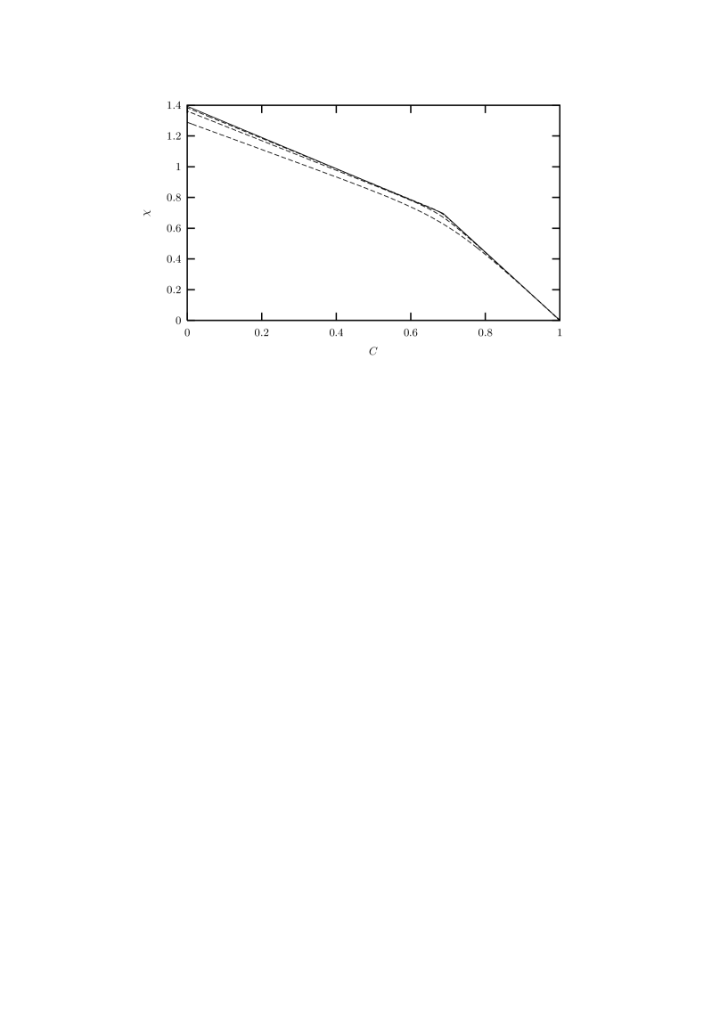
Figure 6.4: (From [146]) Integrated response vs. correlation curves for $T=0.45<T_{d}$. Full line: asymptotic ($\epsilon=0$) analytical curve. Dashed lines (from bottom to top) $\epsilon=0.333$, 0.143, 0.0442. The breaking point corresponds to the plateau of $C(t)$.

The relation between spontaneous and induced fluctuations found in mean-field glassy models, or, equivalently, the relation between $R$ and $C$ in the solutions of Eq. (6.18), is surprisingly simple. Indeed, if the “fast” and “slow” time scales are well separated (i.e. for $T\leq T_{d}$ and $\epsilon\sim 0$, where $\tau_{\alpha}$ is large, see Fig. 6.2), so that the decomposition (6.22) holds, the plot $\chi(C)$ is found to be a broken line:

$$\chi(C)=\frac{1}{T}\;(1-C)\;\theta(C-q_{d})+\left[\frac{1}{T}\;(1-q_{d})+\frac{1}{T_{eff}}(q_{d}-C)\right]\;\theta(q_{d}-C)\;,$$ (6.53)

see Fig. 6.4 and [137] for a review. This broken line has two slopes, $-1/T$ for $C>q_{d}$ (i.e., small $t-t^{\prime}$), and $-1/T_{eff}$ for $C<q_{d}$ (i.e., large $t-t^{\prime}$). Indeed, the first slope gives the relation between $C_{f}$ and $R_{f}$, while the second gives the relation between $C_{s}$ and $R_{s}$:

$$\begin{split}&R_{f}(t)=-\frac{\theta(t)}{T}\frac{dC_{f}}{dt}\ ,\\ &R_{s}(t)=-\frac{\theta(t)}{T_{eff}}\frac{dC_{s}}{dt}\ .\end{split}$$ (6.54)

The breaking-point $q_{d}$, as discussed above, has an interpretation as the self-overlap of the states, i.e. for $t-t^{\prime}$ small the system remains in the same state while for $t-t^{\prime}$ large it jumps to another state. Since $T_{eff}$ is found to be larger than $T$ the second term violates the fluctuation-dissipation theorem. In order to be consistent with the thermodynamic properties one needs to find a single value of $T_{eff}$ in each time regime as defined by the correlation scales of [141].

In presence of a finite drive $\epsilon>0$, $\chi(C)$ is a smooth function of $C$. For $\epsilon\rightarrow 0$ and $T>T_{d}$, the system is in equilibrium and $\chi(C)$ tends to $T^{-1}(1-C)$, i.e. the fluctuation–dissipation relation holds. For $\epsilon\rightarrow 0$ and $T<T_{d}$, $\tau_{\alpha}\rightarrow\infty$ as discussed above, thus the decomposition (6.22) becomes exact and $\chi(C)$ becomes the broken line (6.53), see Fig. 6.4. Defining a FDT violation factor $X\equiv 1/T_{eff}$, one can draw iso-$X$ lines in the $(\epsilon,T)$ plane, see Fig. 6.3, and identify a quasi-equilibrium region defined by $X\sim 1$ (e.g. $X>0.99$). In the latter region the fluctuation–dissipation relation (FDR) holds: it roughly correspond to the linear response region.

The same result for $\chi(C)$, Eq. (6.53), is obtained in the aging dynamics, i.e. for the nonstationary solution of Eq.s (6.14): for $t,t^{\prime}\rightarrow\infty$ the separation (6.16) holds and $\chi(C)$ is given by Eq. (6.53) as in the driven case.

In the case of relaxing glasses the dynamics occurs out of equilibrium because below $T_{d}$ the equilibration time diverges with the size of the system and falls beyond all accessible time-scales. These macroscopic systems then evolve out of equilibrium even if they are in contact with a thermal reservoir, itself in equilibrium at a given temperature $T$, the white bath in Eq. (6.1), due to the interaction between the $N$($\rightarrow\infty$) spins. The effective environment appearing in Eq. (6.12) is self-generated by the system.

In the case of sheared dense liquids, glasses, etc. the systems are driven into an out of equilibrium stationary regime by the external forces, so one does not expect the FDR to hold. However, for $T<T_{d}$, as the dynamics is very slow and non–stationary at zero forcing, it remains slow also for weak forcing, the main effect of a weak forcing being that the system becomes stationary. In this situation the FDR is violated also for small drive, $\epsilon\rightarrow 0$, which is a quite unexpected result.

The suggestive name effective temperature, $T_{eff}$, has been used to parametrize the second slope. The justification is that for mean-field glassy models — and within all resummation schemes applied to realistic ones as well — $T_{eff}$ does indeed behave as a temperature, in the sense that it controls heat flows between systems which are in thermal contact [28, 137, 138].

6.5 Beyond mean-field

The results discussed above follow from Eq.s (6.18), which describe exactly the dynamics of mean field systems and approximate realistic system as well. For realistic systems they can be derived applying suitable resummation and/or approximation schemes.

Indeed, the results described above were obtained in numerical simulations of the slow relaxational dynamics of a number of more realistic glassy systems such as Lennard-Jones mixtures [149], sheared Lennard-Jones mixtures [150, 151] and in a number of other driven low-dimensional models [152].

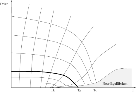
Figure 6.5: (From [146]) Same diagram as in Fig. 6.3, taking into account activated processes. In absence of drive the activated processes restore the equality of $T_{K}$ and $T_{d}$. However below $T_{g}$ the system cannot be equilibrated on the experimental time scale. The curve iso-$\tau_{\alpha}$ corresponding to $\tau_{\alpha}(T_{g})=100$s is drawn as a thick line. Inside the region delimited by this line $\tau_{\alpha}(\epsilon,T)>100$s so the system is not able to reach stationarity and ages. The region defined by $X>0.99$ is again a “near-equilibrium” region that roughly correspond to the linear response region.

However, if one whishes to describe the relaxation of real glasses in finite dimension, more complicated effects have to be taken into account. The problem is that, as discussed in section 1.4, in finite dimensional models metastable states have a finite time and decay by activated processes of barrier crossing. These process are of nonperturbative nature so they are missed by any resummation scheme leading to equations of the class (6.18). These processes are relevant also at equilibrium as they are responsible for the equality of $T_{d}$ and $T_{K}$ in finite dimensional systems, while in mean-field one finds $T_{d}>T_{K}$. Some attempts to describe the equilibrium properties of such processes recently appeared in the literature [11, 12, 13, 14, 46, 47], and have been described in section 1.4 . One of the main results coming from these studies is that the equilibrium dynamics for $T\sim T_{g}$ is expected to be heterogeneous: this means that the relaxation time $\tau_{\alpha}$ is expected to depend on the region inside the sample. This is consistent with experimental and numerical results, see e.g. [48] for a review.

Thus one can expect that heterogeneity is relevant also for the nonequilibrium dynamics yielding a local effective temperature which may depend on space inside the sample. This has indeed very recently proposed and found numerically in finite dimensional spin-glass models and a theory to describe space fluctuations of $T_{eff}$ has been proposed, see e.g. [153, 154] for a detailed discussion.

On the other hand, it seems that in presence of a driving force heterogeneity is somehow reduced. For example, the strecthing parameter of the correlation functions of density fluctuation (which is a measure of the homogeneity of the sample) is found to be an increasing function of the driving force in sheared colloidal suspensions, see e.g. the discussion in [155].

Another important difference follow from the fact that, in finite dimension, due to activated processes, in absence of drive, the system is able to penetrate below the threshold, and is trapped for large times into metastable states from which it can escape only by jumping over some barriers. Then, one expects that an infinitesimal drive is not enough to take the system out of these states. This means that if the drive is small enough the aging dynamics is recovered, as the system can be trapped by metastable states as if the drive were not present, see Fig. 6.5 and [146, 151] for a detailed discussion.

In next chapter, only Langevin equations of the form (6.18) will be considered. The extension of the results that will be presented to glassy systems in finite dimension will require additional work.

Chapter 7 Extension of the fluctuation relation to driven glasses

7.1 Introduction

Relatively few generic results for non-equilibrium systems exist. Two such results that apply to seemingly very different physical situations have been discussed in the last chapters. One is the fluctuation theorem that characterizes the fluctuations of the entropy production over long time-intervals in driven steady states, see chapter 4. Another one is the extension of the fluctuation–dissipation theorem that relates induced and spontaneous fluctuations in equilibrium to the non-equilibrium slow relaxation of glassy systems, see chapter 6. While the former result has been proven for reversible hyperbolic dynamical systems [92, 93] and for the driven stochastic dynamic evolution of an open system coupled to an external environment [108, 156], the latter has only been obtained in a number of solvable mean-field models and numerically in some more realistic glassy systems [140, 141, 149, 150, 151, 152]. As discussed in section 6.4, the modification of the fluctuation–dissipation theorem can be rationalized in terms of the generation of an effective temperature [138, 139]. The expected thermodynamic properties of the effective temperature have been demonstrated in a number of cases [138] (see however footnote 9 in section 6.4).

One may naturally wonder whether these two quite generic results may be included in a common, more generic statement, that reduces to them in the corresponding limits. The scope of this chapter is to discuss this possibility using the very simple working example discussed in section 6.4.2, from which one can very easily reach the ‘driven limit’ and the ‘non-equilibrium relaxational’ case. This project was pioneered by Sellitto [157] who asked the same question some years ago and tried to give it an answer using a stochastic lattice gas with reversible kinetic constraints in diffusive contact with two particle reservoirs at different chemical potentials. Other developments in similar directions have been proposed and analyzed by several authors [158, 159, 160]. They will be discussed in section 7.9.

The fluctuation theorem and the fluctuation–dissipation theorem are related: indeed, for systems which are able to equilibrate in the small entropy production limit ($\sigma_{+}\rightarrow 0$), the fluctuation theorem implies the Green-Kubo relations for transport coefficients, that are a particular instance of the fluctuation–dissipation theorem, see [109, 110, 156] and section 4.4.1. That is, close to equilibrium the fluctuation relation and the fluctuation–dissipation relation are equivalent. It is then natural to wonder what is the fate of the fluctuation theorem if the fluctuation–dissipation is violated even when the driving force is very small, see Fig. 6.4. One can ask if the fluctuation theorem is modified and, more precisely, whether the effective temperature enters its modified version. In particular, this question will arise if the limit of large sampling time, $\tau$ in Eqs. (4.21) and (4.23), is taken after the limit of large system size. The order of the limits is important because a finite size system will always equilibrate with the thermal bath in a large enough time $\tau$. As the fluctuation theorem concerns the fluctuations of $\sigma$ for $\tau\rightarrow\infty$, if one wants to observe nonequilibrium effects, the latter limit has to be taken after the thermodynamic limit.

The idea is to study the relaxational and driven dynamics of the simplest system such that the effective temperature is not trivially equal to the ambient temperature. For a system coupled to a single thermal bath, this happens whenever:

(i) the thermal bath has temperature $T$, but the system is not able to equilibrate with the bath. This is realized by the glassy cases discussed above, provided the sampling time is smaller than the equilibration time; and/or

(ii) the system is very simple (not glassy) but it is set in contact with a bath that is not in equilibrium. One can think of two ways of realizing this fact. One is with a single bath represented by a thermal noise and a memory friction kernel that do not verify the fluctuation-dissipation relation [28]. This situation is realized if one considers the diffusion of a Brownian particle in a complex medium (e.g. a glass, or granular matter) [161, 162, 163]. In this case the medium, which acts as a thermal bath with respect to the Brownian particle, is itself out of equilibrium. Another possibility is to couple the system to a number of equilibrated thermal baths with different time-scales and at different temperatures [139].

These two cases are closely related because, as discussed in chapter 6, at least at the mean-field level, the problem of glassy dynamics can be mapped onto the problem of a single “effective” degree of freedom moving in an out of equilibrium environment. Situations (i) and (ii) are then described by the same kind of equation, namely, a Langevin equation for a single degree of freedom coupled to a non-equilibrium bath, like Eq.s (6.19) and (6.28).

In the following the Langevin equation Eq. (6.28) will be considered. Its main characteristic is that the thermal bath, represented by the functions $g(t-t^{\prime})$ and $\nu(t-t^{\prime})$, is not at equilibrium. This equation reproduces many features of the original equation (6.19) in the driven case, where the functions $\Sigma(t-t^{\prime})$ and $D(t-t^{\prime})$ are stationary.

7.2 Entropy production rate for a nonequilibrium bath

The explicit form of $\sigma_{\tau}$ for the equation of motion (6.28), in the case where $g_{\alpha\beta}(t)=\delta_{\alpha\beta}g(t)$ and $\vec{h}(t)=\vec{h}[\vec{r}(t)]$ is an external nonconservative force that does not explicitly depend on time (e.g., in $d=2$, $\vec{h}=\epsilon(-y,x)$), can be computed following the procedure outlined in section 4.3.1. Note that the functions $\nu(t)$ and $g(t)$ are such that $\nu(t)=\nu(-t)$ while $g(t)$ is proportional to $\theta(t)$, and both decay exponentially in time. The probability distribution of the noise $\vec{\rho}(t)$ is

$${\cal P}[\vec{\rho}(t)]\propto\exp\left[-\frac{1}{2}\int_{-\infty}^{\infty}dtdt^{\prime}\,\rho_{\alpha}(t)\nu^{-1}(t-t^{\prime})\rho_{\alpha}(t^{\prime})\right]\ ,$$ (7.1)

where $\nu^{-1}(t)$ is the operator inverse of $\nu(t)$,

$$\nu^{-1}(t)=\int_{-\infty}^{\infty}\frac{d\omega}{2\pi}\frac{1}{\nu(\omega)}e^{-i\omega t}\ .$$ (7.2)

The probability distribution of $\vec{r}(t)$ is obtained substituting $\vec{\rho}(t)$ obtained from Eq. (6.28) in Eq. (7.1). Then one has

$$\begin{split}{\cal P}[\vec{r}(t)]\propto&\exp\left\{-\frac{1}{2}\int_{-\infty}^{\infty}dtdt^{\prime}\,\left[m\ddot{r}_{\alpha}(t)+\int_{-\infty}^{\infty}dt^{\prime\prime}g(t-t^{\prime\prime})\dot{r}_{\alpha}(t^{\prime\prime})+\frac{\delta V(\vec{r})}{\delta r_{\alpha}(t)}-h_{\alpha}[\vec{r}(t)]\right]\times\right.\\ &\left.\times\nu^{-1}(t-t^{\prime})\left[m\ddot{r}_{\alpha}(t^{\prime})+\int_{-\infty}^{\infty}dt^{\prime\prime\prime}g(t^{\prime}-t^{\prime\prime\prime})\dot{r}_{\alpha}(t^{\prime\prime\prime})+\frac{\delta V(\vec{r})}{\delta r_{\alpha}(t^{\prime})}-h_{\alpha}[\vec{r}(t^{\prime})]\right]\right\}\ .\end{split}$$ (7.3)

With some manipulations it is easy to see that

$$\begin{split}{\cal P}[\vec{r}(-t)]\propto&\exp\left\{-\frac{1}{2}\int_{-\infty}^{\infty}dtdt^{\prime}\,\left[m\ddot{r}_{\alpha}(t)-\int_{-\infty}^{\infty}dt^{\prime\prime}g(t^{\prime\prime}-t)\dot{r}_{\alpha}(t^{\prime\prime})+\frac{\delta V(\vec{r})}{\delta r_{\alpha}(t)}-h_{\alpha}[\vec{r}(t)]\right]\times\right.\\ &\left.\times\nu^{-1}(t-t^{\prime})\left[m\ddot{r}_{\alpha}(t^{\prime})-\int_{-\infty}^{\infty}dt^{\prime\prime\prime}g(t^{\prime\prime\prime}-t^{\prime})\dot{r}_{\alpha}(t^{\prime\prime\prime})+\frac{\delta V(\vec{r})}{\delta r_{\alpha}(t^{\prime})}-h_{\alpha}[\vec{r}(t^{\prime})]\right]\right\}\ .\end{split}$$ (7.4)

To compute $\sigma_{\tau}$ one should consider the probability of a segment of trajectory $[-\tau/2,\tau/2]$ and then send $\tau$ to $\infty$, neglecting all boundary terms. As the functions $g(t)$ and $\nu(t)$ have short range, the trajectories $\vec{r}(t)$ decorrelate exponentially fast in time and up to boundary contributions one can simply truncate the integrals in ${\cal P}[\vec{r}(t)]$ in $t,t^{\prime}\in[-\tau/2,\tau/2]$ to obtain the probability of a segment of trajectory for large $\tau$. Equivalently one can consider the integrals in $(-\infty,\infty)$ and neglect all the boundary terms: then one obtains the entropy production $\sigma_{\infty}$ integrated over the interval $t\in(-\infty,\infty)$ and one can truncate the integral in $[-\tau/2,\tau/2]$ at the end of the computation.

A lot of terms in $\sigma_{\infty}=-\log{\cal P}[\vec{r}(-t)]+\log{\cal P}[\vec{r}(t)]$ trivially cancel. Before discussing the non-trivial terms, define $f(t)=g(t)+g(-t)$ and recall that, from Eq. (6.52)

$$T^{-1}(t-t^{\prime\prime})=\int_{-\infty}^{\infty}\frac{d\omega}{2\pi}\frac{2{\rm Re}\,g(\omega)}{\nu(\omega)}e^{-i\omega(t-t^{\prime\prime})}=\int_{-\infty}^{\infty}dt^{\prime}\nu^{-1}(t-t^{\prime})f(t^{\prime}-t^{\prime\prime})\ .$$ (7.5)

Note that both $f(t)$ and $T^{-1}(t)$ are even function of $t$, and if the bath is in equilibrium at temperature $T$, $T^{-1}(t-t^{\prime})=\delta(t-t^{\prime})/T$.

The terms that do not cancel trivially are the following:

• a “kinetic” term of the form

  $$\begin{split}&\int_{-\infty}^{\infty}dtdt^{\prime}\,\left[m\ddot{r}_{\alpha}(t)\nu^{-1}(t-t^{\prime})\int_{-\infty}^{\infty}dt^{\prime\prime}g(t^{\prime\prime}-t^{\prime})\dot{r}_{\alpha}(t^{\prime\prime})+m\ddot{r}_{\alpha}(t)\nu^{-1}(t-t^{\prime})\int_{-\infty}^{\infty}dt^{\prime\prime}g(t^{\prime}-t^{\prime\prime})\dot{r}_{\alpha}(t^{\prime\prime})\right]=\\ &=\int_{-\infty}^{\infty}dtdt^{\prime}\,m\ddot{r}_{\alpha}(t)\nu^{-1}(t-t^{\prime})\int_{-\infty}^{\infty}dt^{\prime\prime}f(t^{\prime}-t^{\prime\prime})\dot{r}_{\alpha}(t^{\prime\prime})=\int_{-\infty}^{\infty}dtdt^{\prime}\,m\ddot{r}_{\alpha}(t)T^{-1}(t-t^{\prime})\dot{r}_{\alpha}(t^{\prime})\ .\end{split}$$ (7.6)

  If the bath is in equilibrium, this term trivially vanishes as it is the integral of the total derivative of the kinetic energy. It vanishes also for a nonequilibrium bath: indeed, integrating by parts first in $t$ and then in $t^{\prime}$, one has, recalling that $T^{-1}(t)$ is even and short ranged and up to boundary terms:

  $$\begin{split}&\int_{-\infty}^{\infty}dtdt^{\prime}\,\ddot{r}_{\alpha}(t)T^{-1}(t-t^{\prime})\dot{r}_{\alpha}(t^{\prime})=-\int_{-\infty}^{\infty}dtdt^{\prime}\,\dot{r}_{\alpha}(t)\frac{d}{dt}T^{-1}(t-t^{\prime})\dot{r}_{\alpha}(t^{\prime})=\\ &\int_{-\infty}^{\infty}dtdt^{\prime}\,\dot{r}_{\alpha}(t)\frac{d}{dt^{\prime}}T^{-1}(t-t^{\prime})\dot{r}_{\alpha}(t^{\prime})=-\int_{-\infty}^{\infty}dtdt^{\prime}\,\dot{r}_{\alpha}(t)T^{-1}(t-t^{\prime})\ddot{r}_{\alpha}(t^{\prime})=0\ .\end{split}$$ (7.7)

• a “friction” term of the form

  $$\begin{split}\frac{1}{2}\int_{-\infty}^{\infty}dtdt^{\prime}dt^{\prime\prime}dt^{\prime\prime\prime}\,&\big{[}\dot{r}_{\alpha}(t^{\prime\prime})g(t^{\prime\prime}-t)\nu^{-1}(t-t^{\prime})g(t^{\prime\prime\prime}-t^{\prime})\dot{r}_{\alpha}(t^{\prime\prime\prime})-\\ &\dot{r}_{\alpha}(t^{\prime\prime})g(t-t^{\prime\prime})\nu^{-1}(t-t^{\prime})g(t^{\prime}-t^{\prime\prime\prime})\dot{r}_{\alpha}(t^{\prime\prime\prime})\big{]}\ .\end{split}$$ (7.8)

  This term vanishes because the function

  $$K(t^{\prime\prime}-t^{\prime\prime\prime})=\int dtdt^{\prime}\,g(t^{\prime\prime}-t)\nu^{-1}(t-t^{\prime})g(t^{\prime\prime\prime}-t^{\prime})$$ (7.9)

  is even in its argument as one can easily check.

• a “potential” term of the form

  $$\begin{split}\sigma^{V}_{\infty}&=-\int_{-\infty}^{\infty}dtdt^{\prime}dt^{\prime\prime}\,f(t-t^{\prime\prime})\dot{r}_{\alpha}(t^{\prime\prime})\nu^{-1}(t-t^{\prime})\frac{\delta V(\vec{r})}{\delta r_{\alpha}(t^{\prime})}\\ &=-\int_{-\infty}^{\infty}dtdt^{\prime}\,T^{-1}(t-t^{\prime})\dot{r}_{\alpha}(t)\frac{\delta V(\vec{r})}{\delta r_{\alpha}(t^{\prime})}\ .\end{split}$$ (7.10)

  This term is related to the work of the conservative forces. If the bath is in equilibrium, it vanishes being the total derivative of the potential energy. It vanishes also for an harmonic potential $V(\vec{r})=\frac{1}{2}kr^{2}$ because $\frac{\delta V(\vec{r})}{\delta r_{\alpha}(t)}=kr_{\alpha}(t)$ and one can use the same trick used in Eq. (7.7).

• a “dissipative” term which is

  $$\sigma^{eff}_{\infty}=\int_{-\infty}^{\infty}dtdt^{\prime}\,T^{-1}(t-t^{\prime})\dot{r}_{\alpha}(t)h_{\alpha}[\vec{r}(t^{\prime})]=\int_{-\infty}^{\infty}\frac{d\omega}{2\pi}\frac{-i\omega r_{\alpha}(\omega)h_{\alpha}(\omega)}{T_{eff}(\omega)}\ .$$ (7.11)

  This term is related to the work of the dissipative forces. If the bath is in equilibrium at temperature $T$, this is exactly the work of the dissipative forces divided by the temperature of the bath. Otherwise, the work done at frequency $\omega$ is weighted by the effective temperature at the same frequency.

The expression of the total entropy production over the interval $(-\infty,\infty)$ is then

$$\begin{split}\sigma_{\infty}&=\sigma^{V}_{\infty}+\sigma^{eff}_{\infty}=\int_{-\infty}^{\infty}dtdt^{\prime}\,T^{-1}(t-t^{\prime})\dot{r}_{\alpha}(t)\left[-\frac{\delta V(\vec{r})}{\delta r_{\alpha}(t^{\prime})}+h_{\alpha}[\vec{r}(t^{\prime})]\right]\\ &=\int_{-\infty}^{\infty}dtdt^{\prime}\,T^{-1}(t-t^{\prime})\dot{r}_{\alpha}(t)F_{\alpha}(t^{\prime})\ ,\end{split}$$ (7.12)

where $F_{\alpha}(t)=h_{\alpha}[\vec{r}(t)]-\frac{\delta V(\vec{r})}{\delta r_{\alpha}(t)}$ is the total deterministic force acting on the particle at time $t$. The latter expression can be rewritten as

$$\sigma_{\infty}=\int_{-\infty}^{\infty}dt\int_{-\infty}^{t}dt^{\prime}\,T^{-1}(t-t^{\prime})\big{[}\dot{r}_{\alpha}(t)F_{\alpha}(t^{\prime})+\dot{r}_{\alpha}(t^{\prime})F_{\alpha}(t)\big{]}\ ,$$ (7.13)

and this leads to identify the entropy production per unit time $\sigma_{t}$ with

$$\begin{split}&\sigma_{t}=\sigma^{V}_{t}+\sigma^{eff}_{t}=\int_{-\infty}^{t}dt^{\prime}\,T^{-1}(t-t^{\prime})\big{[}\dot{r}_{\alpha}(t)F_{\alpha}(t^{\prime})+\dot{r}_{\alpha}(t^{\prime})F_{\alpha}(t)\big{]}\ ,\\ &\sigma^{V}_{t}=-\int_{-\infty}^{t}dt^{\prime}\,T^{-1}(t-t^{\prime})\left[\dot{r}_{\alpha}(t)\frac{\delta V(\vec{r})}{\delta r_{\alpha}(t^{\prime})}+\dot{r}_{\alpha}(t^{\prime})\frac{\delta V(\vec{r})}{\delta r_{\alpha}(t)}\right]\ ,\\ &\sigma^{eff}_{t}=\int_{-\infty}^{t}dt^{\prime}\,T^{-1}(t-t^{\prime})\big{[}\dot{r}_{\alpha}(t)h_{\alpha}[\vec{r}(t^{\prime})]+\dot{r}_{\alpha}(t^{\prime})h_{\alpha}[\vec{r}(t)]\big{]}\ .\end{split}$$ (7.14)

If the bath is at equilibrium this expression reduces to the work done by the nonconservative forces divided by the temperature of the bath, as expected. Also if the bath is not at equilibrium, but the potential is harmonic, only the contribution $\sigma^{eff}_{t}$ of the nonconservative force has to be taken into account. The reason why the work of the conservative forces produces entropy if the bath is out of equilibrium and the interaction is nonlinear is that the nonlinear interaction couples modes of different frequency which are at different temperature, thus producing an energy flow between these modes; this energy flow is related to the entropy production.

It is also important to remark that boundary terms, that have been neglected in the calculation above, can have important effects on the large fluctuations of $\sigma_{\tau}$ even for $\tau\rightarrow\infty$ [120], as discussed in section 4.4.3.

7.3 Large deviation function for an harmonic potential

The large deviation function in the harmonic case, $V(\vec{r})=\frac{1}{2}kr^{2}$, will now be computed explicitly. In this case $\sigma^{V}_{t}$ is a total derivative, and only the term $\sigma^{eff}_{t}$ related to the nonconservative forces is relevant. This term is proportional to the driving force so it vanishes identically at equilibrium as requested by the empirical prescription of section 4.4.3, so “spurious” contributions coming from boundary terms should be absent. It will be shown that the characteristic function $z(\lambda)$ of $\sigma^{eff}_{t}$ exists, is a convex function of $\lambda$ and verifies the fluctuation relation $z(\lambda)=z(1-\lambda)$.

7.3.1 Equilibrium bath

As a first illustrative example the case of an equilibrium white bath will be considered. The model is a two dimensional harmonic oscillator with potential energy $V(x,y)=\frac{k}{2}(x^{2}+y^{2})$ coupled to a simple white bath in equilibrium at temperature $T$, and driven out of equilibrium by the nonconservative force $\vec{h}=\epsilon(-y,x)$. The equations of motion are

$$\begin{split}&m\ddot{x}_{t}+\gamma\dot{x}_{t}=-kx_{t}-\epsilon y_{t}+\xi_{t}\ ,\\ &m\ddot{y}_{t}+\gamma\dot{y}_{t}=-ky_{t}+\epsilon x_{t}+\eta_{t}\ ,\end{split}$$ (7.15)

where $\xi_{t}$ and $\eta_{t}$ are independent Gaussian white noises with variance $\langle\,\xi_{t}\xi_{0}\,\rangle=\langle\,\eta_{t}\eta_{0}\,\rangle=2\gamma T\delta(t)$. The memory friction kernels $g_{\alpha\beta}(t-s)$ are simply $\delta_{\alpha\beta}g(t-s)=2\delta_{\alpha\beta}\gamma\delta(t-s)\theta(t-s)$ in this case, with $\gamma$ the friction coefficient.

Defining the complex variable $a_{t}=(x_{t}+iy_{t})/\sqrt{2}$ and the noise $\rho_{t}=(\xi_{t}+i\eta_{t})/\sqrt{2}$ the equations of motion can be written as

$$m\ddot{a}_{t}+\gamma\dot{a}_{t}=-\kappa a_{t}+\rho_{t}\ ,$$ (7.16)

where $\kappa=k-i\epsilon$, $\langle\rho_{t}\rho_{0}\rangle=\langle\bar{\rho}_{t}\bar{\rho}_{0}\rangle=0$ and $\langle\rho_{t}\bar{\rho}_{0}\rangle=2\gamma T\delta(t)$. The complex noise $\rho_{t}$ has a Gaussian pdf:

$${\cal P}[\rho_{t}]\propto\exp\left[-\frac{1}{2\gamma T}\int_{-\infty}^{\infty}dt\ \rho_{t}\bar{\rho}_{t}\right]\;.$$ (7.17)

The energy of the oscillator is $H=m\dot{a}\dot{\bar{a}}+ka\bar{a}$, and its time derivative is given by

$$\frac{dH}{dt}=2m{\rm Re}\,\dot{a}_{t}\ddot{\bar{a}}_{t}+2k{\rm Re}\,a_{t}\dot{\bar{a}}_{t}=2\epsilon{\rm Im}\,\dot{a}_{t}\bar{a}_{t}-2\gamma\dot{a}_{t}\dot{\bar{a}}_{t}+2{\rm Re}\,\dot{a}_{t}\bar{\rho}_{t}=W_{t}-\widetilde{W}_{t}\ ,$$ (7.18)

where $W_{t}=2\epsilon{\rm Im}\,\dot{a}_{t}\bar{a}_{t}=\epsilon(x_{t}\dot{y}_{t}-y_{t}\dot{x}_{t})$ is the power injected by the driving force and $\widetilde{W}_{t}=2\gamma\dot{a}_{t}\dot{\bar{a}}_{t}-2{\rm Re}\,\dot{a}_{t}\bar{\rho}_{t}$ is the power extracted by the thermostat.

The entropy production rate (7.14) reduces, as expected, to the injected power divided by the temperature, $\sigma_{t}=\beta W_{t}$, where $\beta=1/T$. One could also consider the entropy production of the bath, $\widetilde{\sigma}_{t}=\beta\widetilde{W}_{t}$; it will be discussed in Appendix 7.12.

The average value of $\sigma_{t}=\beta W_{t}$ is in this case given by $\sigma_{+}=2\epsilon^{2}/(\gamma k)$. To compute the probability distribution function (pdf) of $\sigma_{t}$, it is useful to rewrite it in terms of the complex variable $a_{t}$:

$$\sigma_{\tau}=\int_{-\tau/2}^{\tau/2}dt\ \sigma_{t}=2\epsilon\beta\;{\rm Im}\,\int_{-\tau/2}^{\tau/2}dt\ \dot{a}_{t}\bar{a}_{t}\ .$$ (7.19)

As already discussed, it is easier to compute the characteristic function $z(\lambda)$, Eq. (4.24), in terms of which the fluctuation relation reads $z(\lambda)=z(1-\lambda)$. To leading order in $\tau$ one can neglect all the boundary terms in the integrals. After integrating by parts,

$$\sigma_{\tau}=2\epsilon\beta i\int_{-\tau/2}^{\tau/2}dt\ a_{t}\dot{\bar{a}}_{t}\ ,$$ (7.20)

and recalling that the pdf of the noise is given by Eq. (7.17) one obtains:

$$\langle\exp[-\lambda\sigma_{\tau}]\rangle={\cal N}^{-1}\int d{\cal P}[\rho_{t}]\ \exp\left[-\frac{2i\epsilon\lambda}{T}\int_{-\tau/2}^{\tau/2}dt\ a_{t}\dot{\bar{a}}_{t}\right]\ ,$$ (7.21)

where the normalization factor ${\cal N}=\int d{\cal P}[\rho_{t}]$ is simply given by the numerator calculated at $\lambda=0$.

At the leading order in $\tau$ the function $z(\lambda)$ should not depend on the boundary conditions in Eq. (7.21). Thus, one can impose periodic boundary conditions, $a(\tau/2)=a(-\tau/2)$ and $\dot{a}(\tau/2)=\dot{a}(-\tau/2)$, and expand $a_{t}$ in a Fourier series,

$$a_{t}=\frac{\Delta\omega}{2\pi}\sum_{n=-\infty}^{\infty}a_{n}\ e^{-i\omega_{n}t}\ ,$$ (7.22)

where $\Delta\omega=2\pi/\tau$ and $\omega_{n}=n\Delta\omega$. For $\tau\rightarrow\infty$

$$a_{t}=\int_{-\infty}^{\infty}\frac{d\omega}{2\pi}\ e^{-i\omega t}a_{\omega}\ ,\hskip 30.0pta_{\omega}=\int_{-\infty}^{\infty}dt\ e^{i\omega t}a_{t}\ ,$$ (7.23)

and the equations of motion become

$$a_{\omega}=\frac{\rho_{\omega}}{-\omega^{2}m+\kappa-i\omega\gamma}\equiv\frac{\rho_{\omega}}{D(\omega)}\ .$$ (7.24)

Note that in the limit $\epsilon=0$ the Green function $G(\epsilon,\omega)=1/D(\omega)$ reduces to the one used in section 6.4.2 to compute the violation of the fluctuation-dissipation theorem induced by a nonequilibrium bath. The distribution of the noise is given by

$${\cal P}[\rho_{\omega}]=\exp\left[-\frac{1}{2\gamma T}\int_{-\infty}^{\infty}\frac{d\omega}{2\pi}\ \rho_{\omega}\bar{\rho}_{\omega}\right]\sim\exp\left[-\frac{1}{2\gamma T}\frac{\Delta\omega}{2\pi}\sum_{n=-\infty}^{\infty}\rho_{n}\bar{\rho}_{n}\right]\ .$$ (7.25)

Substituting Eqs. (7.22) and (7.25) into Eq. (7.21) one has

$$\begin{split}\langle\exp[-\lambda\sigma_{\tau}]\rangle&={\cal N}^{-1}\int d\rho_{n}\exp\left[-\frac{\Delta\omega}{2\pi}\sum_{n=-\infty}^{\infty}\left(\frac{|\rho_{n}|^{2}}{2\gamma T}-\frac{2\epsilon\lambda\omega_{n}|\rho_{n}|^{2}}{T|D(\omega_{n})|^{2}}\right)\right]\\ &=\prod_{n=-\infty}^{\infty}\left[1-\frac{4\gamma\epsilon\lambda\omega_{n}}{|D(\omega_{n})|^{2}}\right]^{-1}\end{split}$$ (7.26)

and using Eq. (4.24)

$$z(\lambda)=\lim_{\tau\rightarrow\infty}\frac{1}{\tau}\sum_{n=-\infty}^{\infty}\log\left[1-\frac{4\gamma\epsilon\lambda\omega_{n}}{|D(\omega_{n})|^{2}}\right]=\int_{-\infty}^{\infty}\frac{d\omega}{2\pi}\log\left[1-\frac{4\gamma\epsilon\lambda\omega}{|D(\omega)|^{2}}\right]\ .$$ (7.27)

To show that $z(\lambda)$ verifies $z(\lambda)=z(1-\lambda)$ and hence the fluctuation theorem, note that

$$z(\lambda)-z(1-\lambda)=\int_{-\infty}^{\infty}\frac{d\omega}{2\pi}\log\left[\frac{|D(\omega)|^{2}-4\gamma\epsilon\lambda\omega}{|D(\omega)|^{2}-4\gamma\epsilon(1-\lambda)\omega}\right]$$ (7.28)

and, as $|D(\omega)|^{2}-4\epsilon\gamma\omega=|D(-\omega)|^{2}$, the integrand is an odd function of $\omega$ and the integral vanishes by symmetry. In Appendix 7.10 it is shown that the same result is obtained if one uses Dirichlet boundary conditions (at least for $m=0$, where the computation is feasible); this result supports the approximations made when neglecting all the boundary terms in the exponential. Moreover, in the case $m=0$ the large deviation function $\zeta(p)$ can be explicitly calculated; defining $\tau_{0}=\gamma/k$ and $\sigma_{0}=\sigma_{+}\tau_{0}/2=\epsilon^{2}/k^{2}$, one obtains

$$\zeta(p)=\tau_{0}^{-1}\left[1+p\sigma_{0}-\sqrt{(1+\sigma_{0})(1+p^{2}\sigma_{0})}\right]\ .$$ (7.29)

Thus, for $\tau\rightarrow\infty$ the pdf of $p$ has the form

$$\pi_{\tau}(p)\propto\exp\left[\frac{\tau}{\tau_{0}}f(p,\sigma_{0})\right]\ .$$ (7.30)

Note that $\tau_{0}$ is the decay time of the correlation function of $a_{t}$ [i.e. $\langle a_{t}\bar{a}_{0}\rangle\propto\exp(-t/\tau_{0})$] and $\sigma_{0}$ is the average entropy production over a time $\tau_{0}/2$. Thus, $\tau_{0}$ is the natural time unit of the problem (as expected); remarkably, the function $f$ depends only on $\sigma_{0}$ and not on the details of the model. It would be interesting to see whether the same scaling holds for more realistic models.

In summary, for all driving forces, i.e. all values of $\epsilon$, the fluctuation theorem holds for the entropy production rate (7.14). For a white equilibrium bath this result is a particolar case of the general theorem derived in [156]. The temperature entering the fluctuation theorem is the one of the equilibrated environment with which the system is in contact, although it is not in equilibrium with it, when the force is applied.

One can easily check that the fluctuation-dissipation relation holds in the absence of the drive (see section 6.4.2) but it is strongly violated when the system is taken out of equilibrium by the external force.

7.3.2 Non-equilibrium bath

The calculation will be now generalized to the case of a generic nonequilibrium bath; the equation of motion becomes:

$$m\ddot{a}_{t}+\int_{-\infty}^{\infty}dt^{\prime}\ g(t-t^{\prime})\dot{a}_{t^{\prime}}=-\kappa a_{t}+\rho_{t}\ ,$$ (7.31)

where as before $\kappa=k-i\epsilon$ and $\langle\rho_{t}\bar{\rho}_{0}\rangle=\nu(t)$. The functions $\nu(t)$ and $g(t)$ are now arbitrary (apart from the condition $g(t)=0$ for $t<0$), hence they do not satisfy, in general, Eq. (6.43). As discussed in the introduction of this chapter, Eq. (7.31) provides a model for the dynamics of a confined Brownian particle in an out of equilibrium medium [161, 162, 163].

The dissipated power is given by

$$\frac{dH}{dt}=2\epsilon\;{\rm Im}\,\dot{a}_{t}\bar{a}_{t}-2{\rm Re}\,\int_{-\infty}^{\infty}dt^{\prime}\ g(t-t^{\prime})\dot{a}_{t}\dot{\bar{a}}_{t^{\prime}}+2{\rm Re}\,\dot{a}_{t}\bar{\rho}_{t}=W_{t}-\widetilde{W}_{t}\;,$$ (7.32)

where as in the previous case $W_{t}=2\epsilon{\rm Im}\,\dot{a}_{t}\bar{a}_{t}$ is the power injected by the external force and $\widetilde{W}_{t}=2{\rm Re}\,\int_{-\infty}^{\infty}dt^{\prime}\ g(t-t^{\prime})\dot{a}_{t}\dot{\bar{a}}_{t^{\prime}}-2{\rm Re}\,\dot{a}_{t}\bar{\rho}_{t}$ is the power extracted by the bath.

For this harmonic model $\sigma^{V}_{\tau}$ is a boundary term and Eq. (7.14) gives

$$\sigma^{eff}_{\tau}=-2\epsilon\frac{\Delta\omega}{2\pi}\sum_{n=-\infty}^{\infty}\frac{\omega_{n}|a_{n}|^{2}}{T_{eff}(\omega_{n})}=2\epsilon i\int_{-\tau/2}^{\tau/2}dt\int_{-\tau/2}^{\tau/2}dt^{\prime}\ T^{-1}(t-t^{\prime})a_{t}\dot{\bar{a}}_{t^{\prime}}\ .$$ (7.33)

Note that the last equality holds neglecting boundary terms.

It is interesting to consider also an “alternative” definition of entropy production rate, which has been often used in the literature [84, 104, 105, 106]. It is obtained assuming that the entropy production rate is proportional to the power injected by the external drive, $\sigma^{\Theta}_{t}=\Theta^{-1}W_{t}$, via a parameter $\Theta$ which has the dimension of a temperature. Then, the total entropy production over a time $\tau$ for Eq. (7.31) is given by (neglecting boundary terms)

$$\sigma^{\Theta}_{\tau}=\frac{2\epsilon i}{\Theta}\int_{-\tau/2}^{\tau/2}dt\ a_{t}\dot{\bar{a}}_{t}=-2\epsilon\frac{\Delta\omega}{2\pi}\sum_{n=-\infty}^{\infty}\frac{\omega_{n}|a_{n}|^{2}}{\Theta}\;.$$ (7.34)

Usually, in experiments, $\Theta$ is a free parameter which is adjusted in order for the pdf of $\sigma^{\Theta}$ to verify the fluctuation relation [104, 105, 106]. It is interesting to compute the large deviations function of $\sigma^{\Theta}_{t}$ to check if it verifies the fluctuation relation.

The functions $z_{\Theta}(\lambda)$ and $z_{eff}(\lambda)$ corresponding to the two entropy production rates defined above will now be computed. The computation is straightforward following the strategy of section 7.3.1. In Fourier space, Eq. (7.31) reads

$$a_{\omega}=\frac{\rho_{\omega}}{-m\omega^{2}+\kappa-i\omega g(\omega)}=\frac{\rho_{\omega}}{D(\omega)}\ .$$ (7.35)

The probability distribution of $\rho_{\omega}$ is

$${\cal P}[\rho_{\omega}]=\exp\left[-\int_{-\infty}^{\infty}\frac{d\omega}{2\pi}\frac{|\rho_{\omega}|^{2}}{\nu(\omega)}\right]\ ,$$ (7.36)

thus, as in Eqs. (7.25) and (7.26),

$$\begin{split}\langle\exp[-\lambda\sigma^{\Theta}_{\tau}]\rangle&={\cal N}^{-1}\int d\rho_{n}\exp\left[-\frac{\Delta\omega}{2\pi}\sum_{n=-\infty}^{\infty}\left(\frac{|\rho_{n}|^{2}}{\nu(\omega_{n})}-\frac{2\epsilon\lambda\omega_{n}|\rho_{n}|^{2}}{\Theta|D(\omega_{n})|^{2}}\right)\right]\\ &=\prod_{n=-\infty}^{\infty}\left[1-\frac{2\epsilon\lambda\omega_{n}\nu(\omega_{n})}{\Theta|D(\omega_{n})|^{2}}\right]^{-1}\ ,\end{split}$$ (7.37)

and

$$z_{\Theta}(\lambda)=\int_{-\infty}^{\infty}\frac{d\omega}{2\pi}\log\left[1-\frac{2\epsilon\lambda\omega\nu(\omega)}{\Theta|D(\omega)|^{2}}\right]\ .$$ (7.38)

The function $z_{eff}(\lambda)$ is obtained by substituting $\Theta\rightarrow T_{eff}(\omega)$ with the latter defined in (6.42):

$$z_{eff}(\lambda)=\int_{-\infty}^{\infty}\frac{d\omega}{2\pi}\log\left[1-\frac{4\epsilon\lambda\omega{\rm Re}\,g(\omega)}{|D(\omega)|^{2}}\right]\ .$$ (7.39)

It is easy to prove that $|D(\omega)|^{2}-4\epsilon\omega{\rm Re}\,g(\omega)=|D(-\omega)|^{2}$. Thus, using the same trick used in Eq. (7.28), one can prove that $z_{eff}(\lambda)=z_{eff}(1-\lambda)$. On the contrary, in general, it is not possible to find a value of $\Theta$ such that $z_{\Theta}(\lambda)$ satisfies the fluctuation theorem. It will be shown in the following that this is possible only in some particular situations: essentially, when the dynamics of the particle happens on a single time scale, that corresponds to the experiments cited above.

In conclusion, the fluctuation theorem is satisfied when the entropy production rate is defined using the power injected by the external drive and the temperature of the environment – that is not defined in the case of a nonequilibrium bath – is replaced by the ratio in (6.42).

Note that, as discussed in section 6.4.3, a single nonequilibrium bath can be equivalently represented by many equilibrated baths at different temperatures, eventually acting on different time scales. In Appendix 7.11 it will be shown that also in this case the pdf of the entropy production rate $\sigma^{eff}$ defined in Eq. (7.33) verifies the fluctuation theorem, while the pdf of $\sigma^{\Theta}$ does not.

Moreover, in the latter case one can also consider the entropy production of the baths, defined as the power extracted by each bath divided by the corresponding temperature. This quantity is of interest if one can clearly identify the different thermal baths with which the system is in contact: this is not the case in glassy systems, where the effective temperature is self-generated by the system. Nevertheless, the study of systems of particles coupled to many baths at different temperature is of interest in the study of heat conduction. In Appendix 7.12 it will be proven that the entropy production rate of the baths verifies the fluctuation theorem, at least for $|p|\leq 1$, see the discussion in section 4.4.3 and [120].

7.4 Numerical results

Some numerical simulations of Eq. (7.31) for a particular choice of the nonequilibrium bath and in presence of a linear and nonlinear interaction have been performed. In the linear case, the numerical results confirm the analytical results of the previous section. This finding confirms that the boundary terms neglected in the analytical computation are indeed irrelevant. In the nonlinear case, it is found that the fluctuation relations holds for $\sigma^{eff}_{t}$, as in the linear case.

The simplest non trivial case has been considered, where a massless Brownian particle is coupled to two equilibrated baths: a white (or fast) bath at temperature $T_{f}$ and a colored (or slow) bath with exponential correlation at temperature $T_{s}$. This model has been studied in detail in [139] and is relevant for the description of glassy dynamics when the time scales of the two baths are well separated, as will be discussed in section 7.5. In Appendix 7.11 the general case of an harmonic oscillator coupled to $N$ colored baths is studied. The equations of motion are given by Eq. (7.31) where $g(t)=g_{f}(t)+g_{s}(t)$, $g_{f}(t)=\gamma_{f}\delta(t)$ and $g_{s}(t)=\theta(t)\frac{\gamma_{s}}{\tau_{s}}e^{-\frac{t}{\tau_{s}}}$, or equivalently $g_{f}(\omega)=\gamma_{f}$, $g_{s}(\omega)=\gamma_{s}/(1-i\omega\tau_{s})$. The harmonic potential is replaced by a generic rotationally invariant potential $V(x,y)={\cal V}\left(\frac{x^{2}+y^{2}}{2}\right)={\cal V}(|a|^{2})$. The noise is the sum of a fast and a slow component. Then Eq. (7.31) becomes:

$$\gamma_{f}\dot{a}_{t}+\frac{\gamma_{s}}{\tau_{s}}\int_{-\infty}^{t}dt^{\prime}\ e^{-\frac{t-t^{\prime}}{\tau_{s}}}\dot{a}_{t^{\prime}}=-a_{t}{\cal V}^{\prime}(|a_{t}|^{2})+i\epsilon a_{t}+\rho^{f}_{t}+\rho^{s}_{t}\ ,$$ (7.40)

where $\langle\rho^{f}_{t}\rho^{f}_{t^{\prime}}\rangle=2\gamma_{f}T_{f}\delta(t-t^{\prime})$, $\langle\rho^{s}_{t}\rho^{s}_{t^{\prime}}\rangle=\frac{T_{s}\gamma_{s}}{\tau_{s}}e^{-|t-t^{\prime}|/\tau_{s}}$ and ${\cal V}^{\prime}(x)$ is the derivative of ${\cal V}(x)$ w.r.t. $x$. It is convenient to rewrite this equation in a Markovian form as follows:

$$\begin{cases}&\dot{b}_{t}=-\frac{b_{t}-\upsilon_{t}}{\tau_{s}}+\frac{\gamma_{s}a_{t}}{\tau_{s}^{2}}\ ,\\ &\gamma_{f}\dot{a}_{t}=-a_{t}{\cal V}^{\prime}(|a_{t}|^{2})+i\epsilon a_{t}+\rho^{f}_{t}+b_{t}-\frac{\gamma_{s}a_{t}}{\tau_{s}}\ ,\end{cases}$$ (7.41)

where the auxiliary variable $b_{t}$ has been introduced and $\upsilon_{t}$ is a white noise with correlation $\langle\upsilon_{t}\bar{\upsilon}_{t^{\prime}}\rangle=2\gamma_{s}T_{s}\delta(t-t^{\prime})$. The power injected by the external force is, as usual, $W_{t}=2\epsilon{\rm Im}\,\dot{a}_{t}\bar{a}_{t}$, while the power extracted by the two baths can be written as $\widetilde{W}^{f}_{t}=2{\rm Re}\,\left[\dot{a}_{t}\left(\gamma_{f}\dot{\bar{a}}_{t}-\bar{\rho}^{f}_{t}\right)\right]$ and $\widetilde{W}^{s}_{t}=2{\rm Re}\,\left[\dot{a}_{t}\left(\frac{\gamma_{s}}{\tau_{s}}\bar{a}_{t}-\bar{b}_{t}\right)\right]$.

In the nonlinear case the potential ${\cal V}(|a|^{2})=\frac{g}{2}|a|^{4}$ as been chosen, and the results are compared with the ones obtained for the harmonic case, ${\cal V}(|a|^{2})=k|a|^{2}$. The simulation has been performed for $\epsilon=0.5$, $T_{f}=0.6$, $\gamma_{f}=1$, $T_{s}=2$, $\gamma_{s}=1$ and $\tau_{s}=1$, setting $k=1$ in the linear case and $g=1$ in the nonlinear one. The system (7.41) is numerically solved via a standard discretization of the equations with time step $\delta t=0.01$; the noises are extracted using the routine gasdev of the C numerical recipes.

It is numerically found that $\sigma^{V}_{t}$ and $\sigma^{eff}_{t}$ are uncorrelated (within the precision of the numerical data), so their pdf can be studied separately. Unfortunately, the pdf of $\sigma^{V}_{t}$ is too noisy to allow for a verification of the fluctuation relation in the nonlinear case. This is probably due to the fact that in the linear case $\sigma^{V}_{t}$ reduces to a boundary term; in the nonlinear case it is not a boundary term, but still it might contain “spurious” boundary terms which should be eliminated, see the discussion in section 4.4.3. Indeed, for the accessible values of $\tau$, it is observed that the variance of $\sigma^{V}_{\tau}$ is much larger than its average (while the FR would predict a variance of the order of $\sigma^{V}_{+}$). This large variance can be a finite-$\tau$ effect due to the presence of a boundary term whose fluctuations contribute to the fluctuations of $\sigma^{V}$ but not to the average. If this is the case, the FR should hold at least for $|p|<1$ and very large $\tau$: but the values of $\tau$ can be so large that the FR is unobservable in practice, see [100, 118]. For this reason, in the following the data for $\sigma^{V}$ will not be discussed. The validity of the FR for $\sigma^{V}$ (possibly minus a boundary term) in the nonlinear case remains an open question that should be addressed by future work.

7.4.1 “Effective” entropy production rate

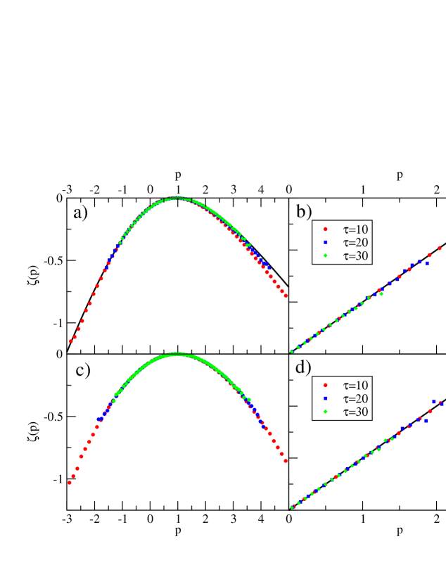
Figure 7.1: pdf of $\sigma^{eff}_{t}$: a) The large deviation function for the harmonic potential at $\tau=10,20,30$; the full line is the analytical result. b) The function $f(p)\equiv[\zeta_{eff}(p)-\zeta_{eff}(-p)]/\sigma^{eff}_{+}$ for the harmonic potential: the fluctuation theorem predicts a straight line with slope 1, represented by a full line. c) The large deviation function for the quartic potential at $\tau=10,20,30$. d) The function $f(p)$ for the quartic potential: also in this case the fluctuation theorem is well verified.

The effective entropy production rate $\sigma^{eff}$, from Eq. (7.14), is given by:

$$\sigma^{eff}_{\tau}=\int_{-\infty}^{t}dt^{\prime}\ T^{-1}(t-t^{\prime})\,2\epsilon{\rm Im}\,\big{[}\dot{a}_{t}\bar{a}_{t^{\prime}}+\dot{a}_{t^{\prime}}\bar{a}_{t}\big{]}\ ,$$ (7.42)

with $T^{-1}(t)$ the Fourier transform of $1/T_{eff}(\omega)$. From Eq. (6.49) the latter is given by

$$\frac{1}{T_{eff}(\omega)}=\frac{\gamma_{f}(1+\omega^{2}\tau_{s}^{2})+\gamma_{s}}{T_{f}\gamma_{f}(1+\omega^{2}\tau_{s}^{2})+T_{s}\gamma_{s}}\;.$$ (7.43)

Thus

$$T^{-1}(t)=\frac{1}{T_{f}}\delta(t)+\frac{\gamma_{s}}{T_{f}\gamma_{f}\tau_{s}^{2}}\left(1-\frac{T_{s}}{T_{f}}\right)\frac{e^{-\Omega|t|}}{2\Omega}\ ,\;\;\;\;\mbox{with}\;\;\;\;\Omega=\frac{1}{\tau_{s}}\sqrt{\frac{T_{f}\gamma_{f}+T_{s}\gamma_{s}}{T_{f}\gamma_{f}}}\ .$$ (7.44)

and $T^{-1}(t)$ decays exponentially for large $t$. Note that, if the bath is at equilibrium, $T_{s}=T_{f}=T$, so one has $T^{-1}(t)=\delta(t)/T$ and $\sigma^{eff}_{t}=2\epsilon{\rm Im}\,\dot{a}_{t}\bar{a}_{t}/T=W_{t}/T$ as expected (recall that by convention $\int_{-\infty}^{t}dt^{\prime}\,\delta(t-t^{\prime})=\frac{1}{2}$).

The data for $\sigma^{eff}_{t}$ are shown in Fig. 7.1. The large deviation function $\zeta_{eff}(p)$ is reported in panel a) for the harmonic and in panel c) for the quartic potential. The average $\sigma^{eff}_{+}$ is equal to $0.332$ in the harmonic case and to $0.276$ in the quartic case. The function $\zeta_{eff}(p)$ converges fast to its asymptotic limit $\tau\rightarrow\infty$ (note that even the data for $\tau\sim 10$ are in quite good agreement with the analytic prediction for the harmonic case). The fluctuation theorem predicts $f(p)\equiv[\zeta_{eff}(p)-\zeta_{eff}(-p)]/\sigma^{eff}_{+}=p$. The function $f(p)$ is reported in panel b) for the harmonic and in panel d) for the quartic potential. In the harmonic case the numerical data are compatible with the validity of the fluctuation theorem, as predicted analytically. Remarkably, the same happens in the quartic case where the analytical prediction is no more available.

These results support the conjecture that, if $\sigma^{V}_{t}$ and $\sigma^{eff}_{t}$ are uncorrelated, the pdf of $\sigma^{eff}$ verifies the fluctuation theorem independently of the form of the potential $V(x,y)$.

7.4.2 “Classical” entropy production rate

It is interesting to investigate numerically also the fluctuations of the entropy production rate $\sigma^{\Theta}$, defined in section 7.3.2 as

$$\sigma^{\Theta}_{t}=\frac{W_{t}}{\Theta}=\frac{2\epsilon}{\Theta}{\rm Im}\,\dot{a}_{t}\bar{a}_{t}\ .$$ (7.45)

Rather arbitrarily $\Theta=T_{f}$ was set in the definition of $\sigma^{\Theta}_{t}$. This reflects what is usually done in numerical simulations, where the dissipated power is divided by the “kinetic” temperature, i.e. the temperature of the fast degrees of freedom. Note that the choice $\Theta=T_{f}$ does not affect the function $\zeta_{\Theta}(p)$ since the variable $p$ is normalized, i.e. $\zeta_{\Theta}(p)\equiv\zeta(p)$ does not depend on $\Theta$, see Eq. (4.21), but it changes the average $\sigma^{\Theta}_{+}$ that is proportional to $\Theta^{-1}$.

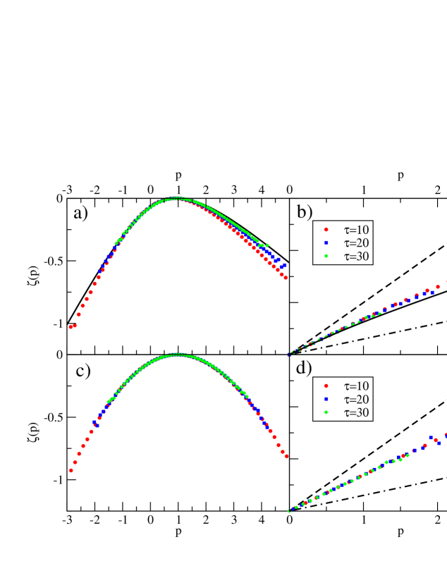
Figure 7.2: pdf of $\sigma^{\Theta}_{t}$: a) The large deviation function for the harmonic potential at $\tau=10,20,30$; the full line is the analytical result. b) The function $f(p)\equiv[\zeta(p)-\zeta(-p)]/\sigma^{T_{f}}_{+}$ for the harmonic potential. The full line is the analytical prediction, the dashed line is the prediction of the fluctuation relation, the dot-dashed line has slope $T_{f}/T_{s}$. c) The large deviation function for the quartic potential at $\tau=10,20,30$. d) The function $f(p)$ for the quartic potential; the dashed line is the fluctuation theorem, the dot-dashed line has slope $T_{f}/T_{s}$.

The data for $\sigma^{\Theta}_{t}$ are reported in Fig. 7.2. The harmonic case is shown in panels a) and b) while the anharmonic case is presented in panels c) and d). The value $\sigma^{T_{f}}_{+}=0.455$ is obtained for the harmonic potential and $\sigma^{T_{f}}_{+}=0.366$ for the quartic one. The large deviation function of $\sigma^{\Theta}_{t}$ agrees very well with the analytical prediction in the harmonic case but it does not verify the fluctuation theorem for $\Theta=T_{f}$, as one can clearly see from the right panels in Fig. 7.2.

Remarkably, in both the harmonic and anharmonic cases the function $f(p)\equiv[\zeta(p)-\zeta(-p)]/\sigma^{T_{f}}_{+}$ is approximately linear in $p$ with a slope $X$ such that $1>X>T_{f}/T_{s}$, i.e. $\zeta(p)-\zeta(-p)\sim X\;p\sigma^{T_{f}}_{+}$. If $f(p)\sim Xp$, one can tune the value of $\Theta$ in order to obtain the fluctuation relation $\zeta(p)-\zeta(-p)=p\sigma^{\Theta}_{+}$, simply choosing $\Theta=\Theta_{eff}=T_{f}/X$, thus defining a single “effective temperature” $\Theta_{eff}\in[T_{f},T_{s}]$. From the data reported in Fig. 7.2 one gets a slope $X\sim 0.66$, that gives $\Theta_{eff}=T_{f}/X\sim 0.9$.

This behavior reflects the one found in some recent experiments [104, 105, 106, 164] in situations where the dynamics of the system happens essentially on a single time scale. This is the case also in the numerical simulation presented here: in Fig. 7.3 (left panel) the autocorrelation function $C(t)={\rm Re}\,\langle a_{t}\bar{a}_{0}\rangle$ of $a_{t}$ (computed in Appendix 7.14) is reported for the harmonic potential. The present simulation refers to the curve with $\tau_{s}=1$, which clearly decays on a single time scale.

In Fig. 7.3 (right panel) the parametric plot $\chi(C)$ (see section 6.4.2) for the same set of parameters, but $\epsilon=0$, is shown. The integrated response is given by $\chi(t)=\int_{0}^{t}dt^{\prime}\,R(t^{\prime})$ and $R(t)$ is computed in Appendix 7.14. For $\tau_{s}=1$, the function $\chi(C)$ has slope close to $-1/T_{f}$ at short times (corresponding to $\chi\sim 0$). For longer times, the slope moves continuously toward $-1/T_{eff}$, with $T_{eff}\sim 1.37$. This value of $T_{eff}$ is of the order of $\frac{\gamma_{f}T_{f}+\gamma_{s}T_{s}}{\gamma_{f}+\gamma_{s}}=1.3$, which means that on time scales of the order of the (unique) relaxation time the two baths behave like a single bath equilibrated at intermediate temperature. This would be exact if the time scales of the two baths were exactly equal.

It is worth to note that in this situation one has $T_{eff}\neq\Theta_{eff}$, that is, the effective temperature that one would extract from the approximate fluctuation relation of Fig. 7.2 is not coincident with the effective temperature obtained from the $\chi(C)$ plot of Fig. 7.3. In particular, $T_{f}<\Theta_{eff}<T_{eff}$: this relation is consistent with the results obtained from the numerical simulation of a sheared Lennard-Jones–like mixture that will be presented below [164], even if the coincidence might be accidental.

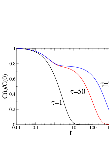
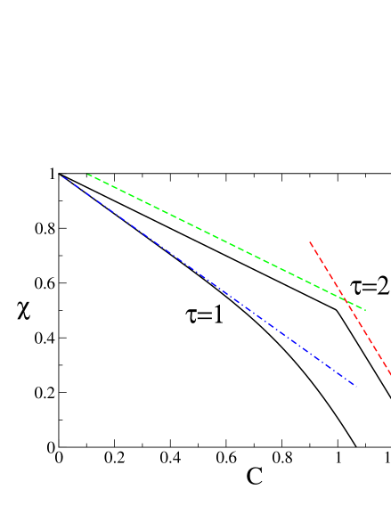
Figure 7.3: (Left) Normalized autocorrelation functions of $a_{t}$ for the harmonic oscillator with $\epsilon=0.5$, $k=1$, $T_{f}=0.6$, $T_{s}=2$, $\gamma_{f}=1$, $\gamma_{s}=k\tau_{s}$ and $\tau_{s}=1,50,250$. (Right) Parametric plot of the integrated response $\chi(t)$ as a function of the correlation function $C(t)$ for the same parameters but $\epsilon=0$. The dot-dashed line has slope $-1/1.37$, the dashed lines have slope $-1/T_{s}$ and $-1/T_{f}$.

7.4.3 Summary of the numerical results

The numerical simulation of the non-linear problem confirms that the fluctuation theorem is satisfied exactly when the entropy production rate $\sigma^{eff}$ is defined using the power injected by the external drive and the temperature of the environment – that is not defined in the case of a nonequilibrium bath – is replaced by the ratio in (6.42).

In situations in which the dynamics of the system happens on a single time scale, a constant effective temperature $\Theta_{eff}$ can be introduced to obtain an approximate fluctuation relation defining the entropy production rate as $W_{t}/\Theta_{eff}$. However, $\Theta_{eff}$ is not necessarily related to the effective temperature $T_{eff}$ that enters the modified fluctuation–dissipation relation, and in the systems considered so far [164] it seems that $\Theta_{eff}<T_{eff}$.

As will be shown in the following, when the dynamics happens on different, well separated, time scales, it is impossible to find a single value $\Theta_{eff}$ such that $\sigma^{\Theta}_{t}=W_{t}/\Theta$ verifies the fluctuation relation.

7.5 Separation of time scales and driven glassy systems

As discussed in chapter 6, in the study of mean-field models for glassy dynamics [28, 139] and when using resummation techniques within a perturbative approach to microscopic glassy models with no disorder, effective equations of motion of the form of Eq. (6.19) are obtained. In the case of a driven mean field system [145, 146], the external force is also present in Eq. (6.19) and after a transient the system becomes stationary for any temperature, i.e. $\mu(t)\equiv\mu$, $\Sigma(t,t^{\prime})=\Sigma(t-t^{\prime})$, and $D(t,t^{\prime})=D(t-t^{\prime})$. The functions $D$ and $\Sigma$ depend on the strength $\epsilon$ of the driving force, e.g. as in Eq. (6.21), and do not satisfy the detailed balance condition. However, it is possible to rewrite Eq.s (6.21) as

$$\begin{split}&D=\frac{p}{2}C^{p-1}+\epsilon^{2}\frac{k}{2}C^{k-1}\equiv D_{0}+\epsilon^{2}D_{1}\ ,\\ &\Sigma=RD^{\prime}_{0}(C)\ ,\end{split}$$ (7.46)

so that $\Sigma$ and $D_{0}$ verify the detailed balance condition. From the expressions (7.46), one can rewrite Eq. (6.19), in the following way:

$$\begin{split}&\dot{\sigma}(t)=-\mu\sigma(t)+\int_{-\infty}^{\infty}dt^{\prime}\ \Sigma(t-t^{\prime})\sigma(t^{\prime})+\rho(t)+\epsilon h(t)\ ,\\ &\left\langle\rho(t)\rho(t^{\prime})\right\rangle=2T\delta(t-t^{\prime})+D_{0}(t-t^{\prime})\ ,\\ &\left\langle h(t)h(t^{\prime})\right\rangle=D_{1}(t-t^{\prime})\ ,\end{split}$$ (7.47)

where $\rho(t)$ and $h(t)$ are two uncorrelated Gaussian variables. Note that $\Sigma$ and $D_{0}$ still depend implicitly on $\epsilon$ as one has to solve the self-consistency equations for $C$ and $R$ and substitute the result in $\Sigma$ and $D_{0}$. However, suppose that the equations have been solved and the solution for $C_{\epsilon}$ and $R_{\epsilon}$ has been plugged in $\Sigma$ and $D_{0}$. If the term proportional to $h(t)$ in Eq. (7.47) is removed, as $\Sigma=RD_{0}^{\prime}(C)$, Eq. (7.47) derives from a Langevin equation where only conservative forces are present [144]. This means that the term corresponding to the external driving is represented only by $h(t)$, and the dissipated power is given by $W(t)=\epsilon h(t)\dot{\sigma}(t)$. Indeed (see Appendix 7.13),

$$\left\langle W\right\rangle=\epsilon^{2}\int_{0}^{\infty}dt\,\dot{R}(t)D_{1}(t)=\epsilon^{2}\frac{k}{2}\int_{0}^{\infty}dt\,\dot{R}(t)C^{k-1}(t)\ ,$$ (7.48)

consistently with the result of [146] where the average of the injected power was explicitly computed for the driven spherical $p$-spin. Thus one obtains an equation that is very similar to Eqs. (7.31) and (7.40), where $\Sigma(C_{\epsilon},R_{\epsilon})$ and $D_{0}(C_{\epsilon})$ represent the nonequilibrium bath, and $\epsilon h(t)$ is the external driving force: and one can prove that the effective entropy production rate

$$\sigma^{eff}(t)=\epsilon\int_{-\infty}^{t}dt^{\prime}\,T^{-1}(t-t^{\prime})\big{[}h(t)\dot{\sigma}(t^{\prime})+h(t^{\prime})\dot{\sigma}(t)\big{]}\ ,$$ (7.49)

where $T_{eff}(\omega)=\frac{2T+D_{0}(\omega)}{2{\rm Re}\,[1+\Sigma(\omega)/(i\omega)]}$, verifies the fluctuation relation, see Appendix 7.13.

As discussed in [146], for small $\epsilon$ and $T>T_{d}$, $R_{\epsilon}$ and $C_{\epsilon}$ verify the fluctuation–dissipation theorem, so the same happens for $D_{0}$ and $\Sigma$, i.e. $T_{eff}(\omega)\equiv T$. The transport coefficient related to the driving force $\epsilon$ approaches a constant value for $\epsilon\rightarrow 0$ (the linear response holds close to equilibrium) and the systems behaves like a “Newtonian fluid”. In this situation, the system behaves as if coupled to a single equilibrium bath (and the fluctuation theorem holds for the entropy production rate $W_{t}/T=\epsilon h(t)\dot{\sigma}(t)/T$).

Below $T_{d}$, the fluctuation-dissipation relation is violated also in the limit $\epsilon\rightarrow 0$ where it is a simple broken line, see Fig. 6.4, with temperature $T$ at short time and $T_{eff}$ at long times. The transport coefficient diverges in this limit: the system is strongly nonlinear and behaves as if coupled to two baths acting on different time scales and equilibrated at different temperatures, and the correct definition of entropy production rate is Eq. (7.49). In the region $\epsilon\sim 0$ and $T<T_{d}$, when the two relaxation scales are well separated, it is possible to separate the “fast” and “slow” parts of the equation of motion (adiabatic approximation). This allows to write all the relations in a particularly simple way.

7.5.1 The adiabatic approximation

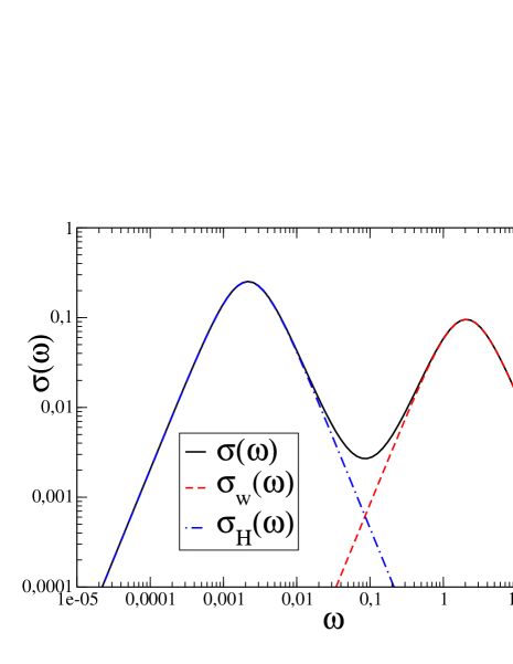
Figure 7.4: Power spectrum of the entropy production rate (full line) as a function of the frequency for the harmonic oscillator with $\epsilon=0.5$, $k=1$, $T_{f}=0.6$, $T_{s}=2$, $\gamma_{f}=1$, $\gamma_{s}=k\tau_{s}$ and $\tau_{s}=250$. The dot-dashed line is the “slow” contribution of $H_{t}$, the dashed line is the “fast” contribution of $w_{t}$.

When a simple system is coupled to a complex bath with two (or more) time scales these are induced into the dynamics of the system. When the time-scales are well separated, an adiabatic treatment is possible in which one separates the dynamic variables in terms that evolve in different time-scales (dictated by the baths) and are otherwise approximately constant.

In this section an adiabatic approach [139] is used to treat simple problems coupled to baths that evolve on different scales. The motivation for studying this type of problems is that the separation of time-scales is self-generated in glassy dynamics, as described above.

The pdf of $\sigma^{\Theta}_{t}$ and $\sigma^{eff}_{t}$ will be studied. The latter satisfies the fluctuation theorem exactly, and the adiabatic approximation does not spoil this feature. The former, instead, does not satisfy the fluctuation theorem in general. The origin of this difference will be evident in the adiabatic approximation.

Consider again the Langevin equation (7.40) with ${\cal V}(|a|^{2})=k|a|^{2}$. In this case, the correlation functions can be calculated explicitly, see Appendix 7.14. In Fig. 7.3 the autocorrelation function, $C(t)=\langle a_{t}\bar{a}_{0}\rangle$, is reported for $\epsilon=0.5$, $k=1$, $T_{f}=0.6$, $T_{s}=2$, $\gamma_{f}=1$, $\gamma_{s}=k\tau_{s}$ and different values of $\tau_{s}$. Clearly, for $k\tau_{s}=\gamma_{s}\gg\gamma_{f}$ two very different time scales –related to the time scales of the two baths– are present. From the plot of Fig. 7.3 one sees that in the case $k\tau_{s}=250\gg\gamma_{f}$ the function $\chi(C)$ is a broken line with slope $-1/T_{f}$ at large $C$ (short times) and $-1/T_{s}$ for small $C$ (large times).

In this situation, the variable $a_{t}$ can be written as the sum of two quasi-independent contributions. Using the construction introduced in [139] one can rewrite the equation of motion (7.40) as

$$\left\{\begin{array}[]{l}\gamma_{f}\dot{a}_{t}=-(k+\gamma_{s}/\tau_{s})a_{t}+i\epsilon a_{t}+\rho^{f}_{t}+h_{t}\;,\\ h_{t}=-\frac{\gamma_{s}}{(\tau_{s})^{2}}\int_{-\infty}^{t}dt^{\prime}\ e^{-\frac{t-t^{\prime}}{\tau_{s}}}a_{t^{\prime}}+\rho^{s}_{t}\;.\end{array}\right.$$ (7.52)

The variable $h_{t}$ is “slow”; considering it as a constant in the first equation, the variable $a_{t}$ will fluctuate around the equilibrium position $a_{h}=h/(k+\gamma_{s}/\tau_{s}-i\epsilon)\equiv H$. The latter will –slowly– evolve according to the second equation in (7.52), in which one can approximate $a_{t^{\prime}}\sim H_{t^{\prime}}$. Defining the –fast– displacement of $a_{t}$ w.r.t. $H_{t}$, $w_{t}\equiv a_{t}-H_{t}$, one obtains the following equations for $(w_{t},H_{t})$:

$$\begin{cases}&\gamma_{f}\dot{w}_{t}=-(k+\gamma_{s}/\tau_{s})w_{t}+i\epsilon w_{t}+\rho^{f}_{t}\ ,\\ &\frac{\gamma_{s}}{\tau_{s}}\int_{-\infty}^{t}dt^{\prime}\ e^{-\frac{t-t^{\prime}}{\tau_{s}}}\dot{H}_{t^{\prime}}=-kH_{t}+i\epsilon H_{t}+\rho^{s}_{t}\ .\end{cases}$$ (7.53)

In this approximation, $a_{t}=H_{t}+w_{t}$ is the sum of two contributions: $w_{t}$ is a “fast” variable which evolves according to a Langevin equation with the fast bath only and a renormalized harmonic constant $k+\gamma_{s}/\tau_{s}$, while $H_{t}$ is a “slow” variable which evolves according to a Langevin equation where the slow bath only appears. In both equations the driving force $\epsilon$ is present, thus one expects both $H_{t}$ and $w_{t}$ to contribute to the dissipation. Note that $w_{t}$ and $H_{t}$ are completely uncorrelated in this approximation.

7.5.2 $\sigma^{V}_{t}$ in the adiabatic approximation

In the adiabatic approximation, one can argue that the term $\sigma^{V}_{t}$ in equation (7.14) becomes a boundary term. Indeed, the function $T^{-1}(t)$, in the adiabatic approximation, becomes

$$T^{-1}(t)=\frac{1}{T_{f}}\delta(t)+T^{-1}_{s}(t)\ ,$$ (7.54)

where the function $T^{-1}_{s}(t)$ is “slow”, see e.g. equation (7.44). Inserting this expression in $\sigma^{V}_{t}$, the first term gives a total derivative. The second term gives

$$\int_{-\infty}^{t}dt^{\prime}\,T^{-1}_{s}(t-t^{\prime})\left[\dot{r}_{\alpha}(t)\frac{\delta V(\vec{r})}{\delta r_{\alpha}(t^{\prime})}+\dot{r}_{\alpha}(t^{\prime})\frac{\delta V(\vec{r})}{\delta r_{\alpha}(t)}\right]\ .$$ (7.55)

Due to the convolution with the “slow” function $T^{-1}_{s}(t)$, the fast components of $r$ are irrelevant in the integral, while for the slow ones it is reasonable to replace $\dot{r}_{\alpha}(t)$ with $\dot{r}_{\alpha}(t^{\prime})$ on the scale $\tau_{s}$ over which $T^{-1}_{s}(t)$ decays. Thus one obtains again a total derivative times the integral of $T^{-1}_{s}(t)$ which is a finite constant. Obviously this is not a rigorous proof and should be checked numerically in concrete cases.

7.5.3 pdf of $\sigma^{eff}_{t}$

The entropy production rate defined in Eqs. (7.33) and (7.42) can be rewritten in terms of $H_{t}$ and $w_{t}$. Recalling that $T^{-1}(t)$ is defined by Eq. (7.44) one obtains (the details of the calculation are reported in Appendix 7.15)

$$\sigma^{eff}_{t}\sim 2\epsilon{\rm Im}\,\left[\frac{\dot{w}_{t}\bar{w}_{t}}{T_{f}}+\frac{\dot{H}_{t}\bar{H}_{t}}{T_{s}}\right]$$ (7.56)

neglecting terms that vanish when $\sigma^{eff}_{t}$ is integrated over time intervals of the order of $\tau_{s}$. This is exactly the entropy production expected for two independent systems.

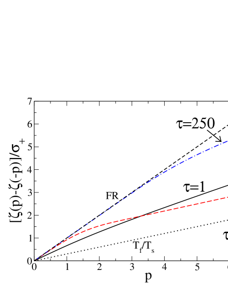
Figure 7.5: The function $[\zeta_{\Theta}(p)-\zeta_{\Theta}(-p)]/\sigma^{\Theta}_{+}$ for the harmonic oscillator with $\epsilon=0.5$, $k=1$, $\Theta=T_{f}=0.6$, $T_{s}=2$, $\gamma_{f}=1$, $\gamma_{s}=k\tau_{s}$ and $\tau_{s}=1,50,250$. The dashed line is a straight line with slope 1, the dotted line has slope $T_{f}/T_{s}=0.3$.

To check that this approximation works well, one can introduce a “power spectrum” $\sigma(\omega)d\omega$ as the contribution coming from frequencies $[\omega,\omega+d\omega]$ to the average entropy production rate, $\sigma^{eff}_{+}=\int_{0}^{\infty}d\omega\,\sigma(\omega)$. From Eq. (7.39) one has

$$\begin{split}&\sigma^{eff}_{+}=\left.\frac{dz_{eff}}{d\lambda}\right|_{\lambda=0}=-\int_{-\infty}^{\infty}\frac{d\omega}{2\pi}\frac{2\epsilon\omega\nu(\omega)}{|D(\omega)|^{2}}\\ &\sigma(\omega)=\frac{1}{2\pi}\left[-\frac{2\epsilon\omega\nu(\omega)}{|D(\omega)|^{2}}+\frac{2\epsilon\omega\nu(-\omega)}{|D(-\omega)|^{2}}\right]=\frac{\epsilon\omega\nu(\omega)}{\pi}\left[\frac{1}{|D(-\omega)|^{2}}-\frac{1}{|D(\omega)|^{2}}\right]\end{split}$$ (7.57)

Substituting the expressions of $\nu(\omega)$ and of $D(\omega)$ appropriate for Eq. (7.40) one gets the power spectrum $\sigma(\omega)$ as a function of $\omega$ which is reported in Fig. 7.4 as a full line. The contributions of $w_{t}$ and $H_{t}$, $\sigma_{w}(\omega)$ and $\sigma_{H}(\omega)$, are obtained inserting in Eq. (7.57) the expression of $\nu(\omega)$ and $D(\omega)$ obtained from the two equations (7.53). They are reported as dashed and dot-dashed lines in Fig. 7.4. One can conclude that, for $k\tau_{s}\gg\gamma_{f}$, the adiabatic approximation holds and $\sigma^{eff}_{t}=\sigma^{w}_{t}+\sigma^{H}_{t}$, with $\sigma^{w}_{t}=2\epsilon{\rm Im}\,\,\dot{w}_{t}\bar{w}_{t}/T_{f}$ and $\sigma^{H}_{t}=2\epsilon{\rm Im}\,\,\dot{H}_{t}\bar{H}_{t}/T_{s}$, and the two contributions are independent. Note that the average dissipation due to $H$ is much larger than the one due to $w$. Finally, one can write:

$$z_{eff}(\lambda)=z^{w}(\lambda)+z^{H}(\lambda)\ ,\hskip 30.0ptz^{w,H}(\lambda)=-\lim_{\tau\rightarrow\infty}\tau^{-1}\log\langle\exp\big{[}-\lambda\sigma^{w,H}\big{]}\rangle\ .$$ (7.58)

Both $z^{w}(\lambda)$ and $z^{H}(\lambda)$ verify the fluctuation theorem, as the two equations of motion (7.53) are particular instances of the general case discussed in section 7.3.2. The function $\zeta_{eff}(p)$ is the Legendre transform of $z_{eff}(\lambda)$ and will verify the fluctuation theorem.

7.5.4 pdf of $\sigma^{\Theta}_{t}$

In the same approximation, $\sigma^{\Theta}_{t}$ is given, for $\Theta=T_{f}$, by

$$\sigma^{T_{f}}_{t}=2\epsilon{\rm Im}\,\left[\frac{\dot{w}_{t}\bar{w}_{t}+\dot{H}_{t}\bar{H}_{t}}{T_{f}}\right]=\sigma^{w}_{t}+\frac{T_{s}}{T_{f}}\sigma^{H}_{t}\ ,\hskip 20.0pt\text{and}\hskip 20.0ptz_{T_{f}}(\lambda)=z^{w}(\lambda)+z^{H}(\lambda T_{s}/T_{f})\ ;$$ (7.59)

the contribution of $H_{t}$ is weighted with the “wrong” temperature, i.e. the temperature of the fast degrees of freedom. Indeed, as already discussed, $z_{\Theta}(\lambda)$ does not verify the fluctuation theorem. The function $f(p)\equiv[\zeta_{\Theta}(p)-\zeta_{\Theta}(-p)]/\sigma^{\Theta}_{+}$, obtained from Eq. (7.38), is reported in Fig. 7.5. As already discussed in section 7.4, when the time scales of the two baths are comparable, $k\tau_{s}\sim\gamma_{f}$, the two baths act like a single bath at temperature $\Theta\in[T_{f},T_{s}]$ and the function $f(p)$ is approximately linear in $p$ with slope $X\in[T_{f}/T_{s},1]$. When the time scales are well separated, $k\tau_{s}\gg\gamma_{f}$, the adiabatic approximation holds; in this situation it turns out, from the exact computation of $\zeta_{\Theta}(p)$, that the function $f(p)$ has slope $\sim 1$ for small $p$ and has slope $T_{f}/T_{s}$ for large $p$ (see Fig. 7.5). These results will be compared with numerical simulations of Lennard-Jones systems below.

7.6 Green-Kubo relations

The Green-Kubo relations for transport coefficients, that are a particular form of the fluctuation–dissipation theorem, follow from the fluctuation relation, as discussed in section 4.4.1. In this section a way to link the modified fluctuation theorem – in which the external bath temperature is replaced by the (frequency dependent) effective temperature of the unperturbed system – to the modification of the fluctuation–dissipation relation will be discussed.

Note that even out of equilibrium one can define a flux ${\cal J}_{t}$ using $\sigma_{t}$ as a “Lagrangian”, see Eq. (4.37) and [84]:

$${\cal J}_{t}=\frac{\partial\sigma_{t}}{\partial E}\ .$$ (7.60)

Close to equilibrium $\sigma_{t}$ is given by Eq. (4.31) and ${\cal J}_{t}=J_{t}/T$. If, in the absence of a drive, the system has a non trivial effective temperature, the entropy production rate should be defined as in Eqs. (7.33) and (7.42). Then the flux ${\cal J}_{t}$ is given by

$${\cal J}_{t}=\frac{\partial\sigma^{eff}_{t}}{\partial\epsilon}=4\,{\rm Im}\,\int_{-\infty}^{t}dt^{\prime}T^{-1}(t-t^{\prime})\dot{a}_{t}\bar{a}_{t^{\prime}}=2\int_{-\infty}^{t}dt^{\prime}T^{-1}(t-t^{\prime})[\dot{y}_{t}x_{t^{\prime}}-\dot{x}_{t}y_{t^{\prime}}]\ .$$ (7.61)

The fluctuation theorem for $\sigma^{eff}$ implies then a Green-Kubo relation for ${\cal J}_{t}$:

$$\langle{\cal J}\rangle_{\epsilon}=\epsilon\int_{0}^{\infty}dt\ \langle{\cal J}_{t}{\cal J}_{0}\rangle_{\epsilon=0}+o(\epsilon^{2})\ .$$ (7.62)

The physical meaning of the latter relation becomes clear if one writes the flux ${\cal J}_{t}$ in the adiabatic approximation discussed in the previous section; from Eq. (7.56):

$${\cal J}_{t}=2{\rm Im}\,\left[\frac{\dot{w}_{t}\bar{w}_{t}}{T_{f}}+\frac{\dot{H}_{t}\bar{H}_{t}}{T_{s}}\right]=\frac{J^{w}_{t}}{T_{f}}+\frac{J^{H}_{t}}{T_{s}}\ ,$$ (7.63)

and Eq. (7.62) becomes

$$\frac{\langle J^{w}\rangle_{\epsilon}}{T_{f}}+\frac{\langle J^{H}\rangle_{\epsilon}}{T_{s}}=\frac{\epsilon}{T_{f}^{2}}\int_{0}^{\infty}dt\ \langle J^{w}_{t}J^{w}_{0}\rangle_{\epsilon=0}+\frac{\epsilon}{T_{s}^{2}}\int_{0}^{\infty}dt\ \langle J^{H}_{t}J^{H}_{0}\rangle_{\epsilon=0}+o(\epsilon^{2})\ .$$ (7.64)

Indeed, in the adiabatic approximation the Green-Kubo relation holds separately for $J^{w}_{t}$ (with temperature $T_{f}$) and for $J^{H}_{t}$ (with temperature $T_{s}$). Eq. (7.62) encodes the two contributions and holds even when the adiabatic approximation does not apply and the contributions of the “fast” and of the “slow” modes is not well separated.

Note that the “classical” Green-Kubo relation involves the total flux $J_{t}=J^{w}_{t}+J^{H}_{t}$. For the latter one has, in the adiabatic approximation,

$$\begin{split}\langle J_{t}\rangle_{\epsilon}&=\langle J^{w}_{t}\rangle_{\epsilon}+\langle J^{H}_{t}\rangle_{\epsilon}=\frac{\epsilon}{T_{f}}\int_{0}^{\infty}dt\ \langle J^{w}_{t}J^{w}_{0}\rangle_{\epsilon=0}+\frac{\epsilon}{T_{s}}\int_{0}^{\infty}dt\ \langle J^{H}_{t}J^{H}_{0}\rangle_{\epsilon=0}\\ &=\epsilon\int_{0}^{\infty}dt\left[\frac{\langle J^{w}_{t}J^{w}_{0}\rangle_{\epsilon=0}}{T_{f}}+\frac{\langle J^{H}_{t}J^{H}_{0}\rangle_{\epsilon=0}}{T_{s}}\right]\sim\epsilon\int_{0}^{\infty}dt\frac{1}{T_{eff}(t)}\langle J_{t}J_{0}\rangle_{\epsilon=0}\ .\end{split}$$ (7.65)

The latter relation is the generalization of the Green-Kubo formula that comes from the generalized FDR discussed in section 6.4.3. It is closely related, but not equivalent, to Eq. (7.62).

7.6.1 The Green-Kubo relation for driven glassy systems

Equations (7.62) and (7.65) cannot be applied straightforwardly to driven glassy systems as for these systems the correlation function $\langle J_{t}J_{0}\rangle_{\epsilon}$ is not stationary at $\epsilon=0$ below $T_{d}$. Indeed, the relaxation time of the latter diverges as $\epsilon\rightarrow 0$ and at some point falls outside the experimentally accessible range: the system will not be able to reach stationarity on the experimental time scales and will start to age indefinitely.

The problem is that in Eq. (7.47) the functions $\Sigma(t-t^{\prime})$ and $D_{0}(t-t^{\prime})$, that define the thermal bath, depend strongly on $\epsilon$ through the functions $C$ and $R$ which are determined self-consistently. However, the Green-Kubo relations above have been obtained sending the driving force $\epsilon\rightarrow 0$ keeping the thermal bath fixed. This means that in Eq. (7.47) one should send the term $\epsilon h\rightarrow 0$ keeping fixed the functions $\Sigma$ and $D_{0}$. For $\epsilon\sim 0$, the main contribution to the $\epsilon$-dependence of the dynamics of $\sigma(t)$ comes from the $\epsilon$-dependence of $\Sigma$ and $D_{0}$, so removing the term $\epsilon h$ at fixed $\Sigma$ and $D_{0}$ does not affect too much the correlation function $\langle J_{t}J_{0}\rangle_{\epsilon}$ if $\epsilon$ is small. Thus, for small $\epsilon$, one can write the Green-Kubo relations in the form

$$\langle J_{t}\rangle_{\epsilon}\sim\epsilon\int_{0}^{\infty}dt\frac{1}{T_{eff}(t)}\langle J_{t}J_{0}\rangle_{\epsilon}\ ,$$ (7.66)

even if the limit $\epsilon\rightarrow 0$ is not well defined. An analogous relation will be obtained from Eq. (7.62) (which is equivalent to the fluctuation theorem in the Gaussian approximation) within the same approximation. The latter relations can be tested in numerical simulations as well as in experiments.

7.7 Slow periodic drive and effective temperature

A lesson one learns from the previous calculations (see e.g.  Fig. 7.4) is that the work done at large frequencies is overwhelmingly larger than that done at very low frequencies – precisely the one that one wishes to observe in order to detect effective temperatures. One way out of this is to choose a perturbation that does little work at high frequencies: a periodically time-dependent force that derives from a potential $\cos(\Omega t){\tilde{V}}(r)$, with $1/\Omega$ of the order of timescale of the slow bath $\tau_{s}$. In the following a one dimensional system will be discussed, the generalization is straightforward.

Consider a single degree of freedom $r$ moving in a time-independent potential $V(r)$ and subject to a periodically time-dependent field $\cos(\Omega t){\tilde{V}}(r)$, and in contact with a ‘fast’ and a ‘slow’ bath with friction kernel, thermal noise and temperature $(\rho^{f},g_{f},T_{f})$ and $(\rho^{s},g_{s},T_{s})$, respectively:

$$m\ddot{r}(t)+\int_{-\infty}^{t}dt^{\prime}\;\big{[}g_{f}(t-t^{\prime})+g_{s}(t-t^{\prime})\big{]}{\dot{r}}(t^{\prime})=-\frac{\partial V}{\partial r(t)}+\rho^{f}(t)+\rho^{s}(t)-\cos(\Omega t)\frac{\partial{\tilde{V}}}{\partial r(t)}\;,$$ (7.67)

The time scale of the time dependent field $1/\Omega$ is of the same order as that of the ‘slow’ bath. The work in an interval of time $(0,\tau)$ done by the time-dependent potential is:

$$W_{\tau}=-\int_{0}^{\tau}\;\cos(\Omega t^{\prime})\;\frac{\partial{\tilde{V}}}{\partial r}\;\dot{r}\;dt^{\prime}=-{\tilde{V}}(\tau)+{\tilde{V}}(0)+\Omega\int_{0}^{\tau}\;\sin(\Omega t^{\prime})\;{\tilde{V}}\;dt^{\prime}\ .$$ (7.68)

Only the last term grows with the number of cycles, so for long times one can neglect the first two. Now, integrating (7.67) by parts, one has:

$$m\ddot{r}(t) = -\int_{-\infty}^{t}dt^{\prime}\;g_{f}(t-t^{\prime}){\dot{r}}(t^{\prime})-\frac{\partial V}{\partial r(t)}+\rho^{f}+h(t)-\hat{h}(t)\frac{\partial{\tilde{V}}}{\partial r(t)}$$ (7.69)

$$h(t) \equiv -\int_{-\infty}^{t}dt^{\prime}\;g_{s}(t-t^{\prime})r(t^{\prime})+\rho^{s}(t)\;.$$ (7.70)

where $\hat{h}(t)=\cos(\Omega t)$. In the adiabatic limit when both the timescales of the slow bath and the period $1/\Omega$ of the potential $\tilde{V}$ are large, $h(t)$ and $\hat{h}(t)$ are quasi-static. Hence, $r$ has a fast evolution given by Eq. (7.69) with $h,\hat{h}$ fixed and it reaches a distribution [139]

$$P(r/h,\hat{h})=\frac{e^{-\beta_{f}\left(V+\hat{h}{\tilde{V}}+g_{f}(0)\frac{r^{2}}{2}-hr\right)}}{\int\;dr\;e^{-\beta_{f}\left(V+\hat{h}{\tilde{V}}+g_{f}(0)\frac{r^{2}}{2}-hr\right)}}\;.$$ (7.71)

The denominator defines $Z(h,\hat{h})$ and $F(h,\hat{h})\equiv-\beta_{f}^{-1}\log Z(h,\hat{h})$. Note that $F(h,\hat{h}(t))$ is periodically time-dependent through $\hat{h}$. The approximate evolution of $h$ is now given by Eq. (7.70) with the replacement of $r$ in the friction term by its average $\frac{\partial F(h,\hat{h})}{\partial h}$ with respect to the fast evolution:

$$h(t)=\int_{-\infty}^{t}dt^{\prime}\,g_{s}(t-t^{\prime})\frac{\partial F(h,\hat{h})}{\partial h}(t^{\prime})+\rho^{s}(t)\;.$$ (7.72)

Equation (7.72) is in fact a generalized Langevin equation for a system coupled to a (slow) bath of temperature $T_{s}$. Indeed, it can be shown [139] to be equivalent to a set of degrees of freedom $y_{i}$ evolving according to the ordinary Langevin equation:

$$\left[m_{j}\frac{d^{2}}{dt^{2}}+\gamma_{j}\frac{d}{dt}+\Omega_{j}\right]y_{j}=\xi_{j}(t)-\frac{\partial F\left(\sum_{j}A_{j}y_{j}\right)}{\partial y_{j}}$$ (7.73)

with $\langle\xi_{i}(t)\xi_{j}(t^{\prime})\rangle=2T_{s}\gamma_{j}\delta_{ij}\delta(t-t^{\prime})$, provided that the Fourier transforms $g_{s}(\omega)$ an $\nu_{s}(\omega)$ of friction kernel and noise autocorrelation can be written as:

$$\begin{split}&g_{s}(\omega)=\sum_{j}\frac{A^{2}_{j}}{m_{j}(\omega-\omega_{j}^{+})(\omega-\omega_{j}^{-})}\ ,\\ &\nu_{s}(\omega)=2T_{s}\sum_{j}\frac{\gamma_{j}A^{2}_{j}}{m^{2}_{j}(\omega-\omega_{j}^{+})(\omega-\omega_{j}^{-})(\omega+\omega_{j}^{+})(\omega+\omega_{j}^{-})}\ ,\end{split}$$ (7.74)

where $\omega^{\pm}_{j}$ are the roots of $-m_{j}\omega^{2}+i\gamma_{j}\omega+\Omega_{j}=0$.

Within the same approximation leading to (7.72), the average of $\tilde{V}(r)$ over a time window $\Delta$ that is long compared to the short timescale, but sufficiently slow that one can consider that $h$ and $\hat{h}$ are constant is

$$\int_{t}^{t+\Delta}\;\tilde{V}(r(t^{\prime}))\;dt^{\prime}\sim\Delta\int\;dr\;P(r/h,\hat{h})\;\tilde{V}(r)=\Delta\frac{\partial F(h,\hat{h})}{\partial\hat{h}}$$ (7.75)

so that one obtains for the work:

$$W_{\tau}\sim\Omega\int_{0}^{\tau}\sin(\Omega t^{\prime})\frac{\partial F(h,\hat{h}(t^{\prime}))}{\partial\hat{h}}dt^{\prime}=-\int_{0}^{\tau}\;\frac{\partial F(h,\hat{h}(t^{\prime}))}{\partial t^{\prime}}dt^{\prime}$$ (7.76)

which tells that for long time intervals the work done by the original time-dependent potential $\tilde{V}$ is indeed the same as the work done by the time-dependent effective potential $F$ in (7.72).

The fluctuation theorem then holds for the distribution of this work, with a single temperature $T_{s}$. One concludes that the distribution of work due to a slow perturbation satisfies the fluctuation theorem with only the slow temperature, and can be hence used experimentally to detect it.

The simplest application of the above general result is obtained considering $\tilde{V}(r)=\tilde{h}r$ and $V(r)=kr^{2}$. Then, grouping together the two noises in a single noise with friction $g=g_{f}+g_{s}$ and correlation $\nu=T_{f}\nu_{f}+T_{s}\nu_{s}$ as described in section 6.4.3, Eq. (7.67) becomes simply

$$m\ddot{r}(t)+\int_{-\infty}^{t}dt^{\prime}\,g(t-t^{\prime})\dot{r}(t^{\prime})=-kr(t)+\rho(t)+\tilde{h}\cos(\Omega t)\ .$$ (7.77)

This equation describes for instance the motion of a Brownian particle moving in an out of equilibrium environment and trapped by an harmonic potential whose center oscillates at frequency $\Omega$. A concrete experimental realization of this setting has been already considered in [161]: Silica beads of $\sim 2\mu$m diameter were dispersed in a solution of Laponite (a particular clay of $\sim 30$nm diameter) and water. The Laponite suspension forms a glass for large enough concentration of clay and provides the nonequilibrium environment. The Silica beads are Brownian particles diffusing in such environment. They can be trapped by optical tweezing, and the center of the trap can oscillate with respect to the sample if the latter is oscillated through a piezoelectric stage. In [161] the mobility and diffusion of tracer particles were measured obtaining an estimate of $T_{eff}(\Omega)$. To check the fluctuation relation one has to perform a measurement of the work done by the trap on the tracers. Indeed, the work dissipated in $(0,\tau)$ is linear in $r(t)$ so it should be possible to measure it simply through the measurement of $r(t)$:

$$W_{\tau}=\Omega\tilde{h}\int_{0}^{\tau}dt^{\prime}\sin(\Omega t^{\prime})r(t^{\prime})\ ;$$ (7.78)

note that, as $W_{\tau}$ is linear in $r(t)$, it is a Gaussian variable. With a simple calculation one finds

$$\lim_{\tau\rightarrow\infty}\frac{\langle(W_{\tau}-\langle W_{\tau}\rangle)^{2}\rangle}{2\langle W_{\tau}\rangle}=\frac{\nu(\Omega)}{2{\rm Re}\,g(\Omega)}=T_{eff}(\Omega)$$ (7.79)

This means that the (Gaussian) pdf of $\sigma^{eff}_{\tau}=W_{\tau}/T_{eff}(\Omega)$ satisfies the fluctuation relation. If the two baths are modeled as in section 7.4 with $k\gamma_{s}=\tau_{s}\gg\gamma_{f}$ one has $T_{eff}(\Omega)=T_{s}$ for $\Omega\tau_{s}<1$, see Eq. (7.43). The measurement of the distribution of the work (7.78) allows for the measurement of $T_{s}$. Note that other experimental settings described by the same equations should exist.

7.8 Numerical simulation of a binary Lennard–Jones mixture

It is interesting to test the predictions above in a numerical simulation of a realistic model for a glassy system, like the ones considered in [126, 127, 149]. The predictions obtained from the solution of the dynamics of $p$-spin models have been succesfully tested in the numerical simulations of these models. Indeed, on the space-time scales of the numerical simulations (which are very small) the glass transition is very similar to the mean-field one, see the discussion in section 1.4. On these scales, the glass transition $T_{g}$ reflects the dynamical transition $T_{d}$ of $p$-spin models: the numerical results are very well described by mode-coupling equations of the form (6.18), see e.g.  [126, 135, 136], and a violation of the fluctuation–dissipation theorem of the form (6.53) is observed [149]. The driven dynamics of these systems has been investigated in [150, 151, 166] where a uniform velocity gradient $\gamma$ was applied on a Lennard-Jones binary mixture, and the results described in section 6.3 were very well reproduced by the numerical data.

Thus, it is interesting to see if the generalization of the fluctuation relation proposed above holds for these systems below $T_{g}$ and for $\gamma\sim 0$. Note that a possible generalization of the FR, of the form

$$\zeta_{\infty}(p)-\zeta_{\infty}(-p)=Xp\sigma_{+}\ ,$$ (7.80)

with $X<1$, was proposed in [95, 112, 129] in the context of chaotic dynamical systems, see the discussion in section 5.7. It has also been proposed to define $\Theta_{eff}\equiv T/X$ as the “temperature” in nonequilibrium steady states [84]. However, up to now numerical studies of the FR have been performed only in the high temperature region ($T\gg T_{g}$), where $X=1$.

Eq. (7.80) was shown to hold approximately if the time scales of the two baths are not well separated in section 7.4. The numerical data that will be presented in this section [164] show that indeed (7.80) is satisfied by $\zeta_{\infty}(p)$ below $T_{g}$. Unfortunately, (i) it seems that the proposed connection between Eq. (7.80) and phase space properties is not confirmed by the numerical data, and (ii) a regime in which the time scales are well separated is not accessible due to limited computational power, so that the predictions of section 7.4 could not be completely tested. These open points will hopefully be addressed by future works.

7.8.1 The model

The investigated system is a 80:20 binary mixture of $N$ particles in $d=3$ of equal mass $m$ interacting via a soft sphere potential

$$V_{\alpha\beta}(r)=\epsilon_{\alpha\beta}\left(\frac{\sigma_{\alpha\beta}}{r}\right)^{12}\ ,$$ (7.81)

$\alpha,\beta\in[A,B]$. It is very similar to model II of section 5.3, and the parameters $\epsilon_{\alpha\beta}$ and $\sigma_{\alpha\beta}$ are the same as in section 5.3. This system has been introduced and characterized in equilibrium by De Michele et al [127] as a modification of the standard LJ Kob-Andersen mixture [126] that is known to avoid crystallization on very long time scales, and hence to be a very good model of glass former; it has been chosen because the soft sphere potential can be cut at very short distance ($1.5\sigma_{AA}$) allowing the system to be very small.

A shear flow is applied to the system along the $x$ direction with a gradient velocity field along the $y$ axis. The shear flow was chosen instead of the constant force of section 5.3 for two reasons. On one hand, it makes easier a comparison with the existing literature concerning the driven glassy regime [150, 151, 166]; on the other hand, the shear flow couples directly with the cooperative structural rearrangemens which are responsible for the glassy behavior, while the constant force used in section 5.3 couples to single-particle diffusion.

The particles are confined in a cubic box with Lees-Edwards boundary conditions and the molecular dynamics simulation is performed using SLLOD equations of motion [80]:

$$\begin{cases}&\dot{q}_{i}=\frac{p_{i}}{m}+\gamma q_{yi}\hat{x}\,,\\ &\dot{p}_{i}=F_{i}(q)-\gamma p_{yi}\hat{x}-\alpha({\underline{p}},{\underline{q}})p_{i}\,,\end{cases}$$ (7.82)

where $F_{i}(q)=-\partial_{q_{i}}V(q)$ and $\alpha$ is a thermostat which fixed the kinetic temperature $T$, as discussed in section 5.3. The equation of motion are discretized following the procedure described in section 5.3. The entropy production rate is defined as the dissipated power $W$ divided by the kinetic temperature $T$:

$$\sigma(p,q)=\frac{W(p,q)}{T}=-\frac{\gamma P_{xy}(p,q)}{T},$$ (7.83)

where $P_{xy}(p,q)=\sum_{i}[p_{xi}p_{yi}+q_{yi}F_{xi}(q)]$ is the $xy$ component of the stress tensor [80]. As in section 5.3, all the quantities are reported in units of $m$, $\epsilon_{AA}$ and $\sigma_{AA}$. In these units the integration step is $dt=0.005$. The density is fixed to $\rho=1.2$ to compare with [126, 127, 149].

The main problem is in chosing the size of the system, for the following reasons:

1. If $N$ is too small, it is easy for the system to crystallize, especially in presence of shear. Thus one has to choose $N$ large in order to avoid spurious fluctuations due to nucleation of crystals.

2. On the other hand, the fluctuations of $p$ scale as $\exp[-Nf(p)]$, so if $N$ is too large it is impossible to observe negative values of $p$ which are needed to test Eq. (7.80).

3. One could solve this problem by choosing a very large $N$ ($\sim 1000$, as in [150, 151]) and looking to the fluctuations of $\sigma$ in a small volume inside the sample, following [98, 165]. An attempt in this direction was made, but it turned out that it was difficult to give a good definition of local entropy production rate.

The value $N$=66, which is large enough to avoid crystallization and small enough to allow for the observation of negative values of $p$, was chosen. However, to reach the asymptotic regime one has to integrate $\sigma$ over a time interval $\tau\sim 10\tau_{\alpha}$, see the results of chapter 5. This means that for large $\tau_{\alpha}$, i.e. for $\gamma\sim 0$ and $T<T_{g}$, to obtain a reasonably large number of values of $p$, enough to observe large deviations, one needs to simulate Eq. (7.82) for a very large total time. This strongly limits the values of $\gamma$ and $T$ which are accessible to investigation, and in particular completely rules out, for the large system considered here, the region where the “fast” and “slow” time scales are well separated.

It seems that the observation of curves like the one reported in Fig. 7.5 in numerical simulations of glassy systems is a very difficult task. Probably some difficulties can be avoided considering e.g. the diffusion of a tracer particle in the sample [151], but this is a different physical situation that is left for future investigation.

7.8.2 Results

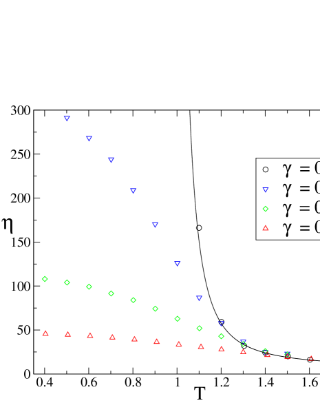
Figure 7.6: Viscosity as a function of temperature for different values of $\gamma$. The continuous line is a fit to a Vogel-Tamman-Fulcher law, $\eta(T)=\eta_{\infty}\exp(\frac{AT_{0}}{T-T_{0}})$ with $\eta_{\infty}=5.2$, $A=0.99$, $T_{0}=0.85$.

In Fig. 7.6 the viscosity $\eta\equiv\langle P_{xy}\rangle/\gamma$ is reported as a function of the temperature $T$ for different values of the shear rate $\gamma$. At $\gamma=0$ the viscosity seems to diverge at a temperature $T_{0}\sim 0.85$; however, the system can be equilibrated only down to $T\sim 1.1$, that provides an estimate for the glass transition temperature $T_{g}$. For $\gamma>0$ the system becomes stationary and the viscosity is finite at all temperatures, even below $T_{0}$.

Very long simulation runs (up to $2\cdot 10^{9}$ time steps) have been performed to measure the pdf of the entropy production rate at different temperatures along the line $\gamma=0.03$. During each run, $p(t)$, given by Eq. (4.21), has been measured on subsequent time intervals of duration $\tau$. From this dataset, the histograms of $\pi_{\tau}(p)$ and the large deviation function $\zeta_{\tau}(p)$ defined in Eq. (4.23) are obtained, following the procedure described in section 5.4.

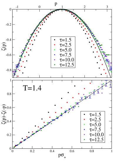
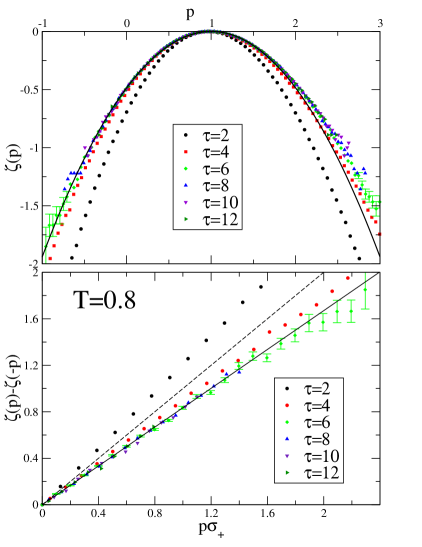
Figure 7.7: (Left) Top: the large deviation function $\zeta_{\tau}(p)=\tau^{-1}\log\pi_{\tau}(p)$ as a function of $p$ for different values of $\tau$ at $T=1.4>T_{g}$ and $\gamma=0.03$. Error bars are smaller than the symbols except on the tails: they are reported only for $\tau=7.5$ to avoid confusion. The line is a Gaussian fit to the data with $\tau>5$ for $p\in[0,2]$. Bottom: $\zeta_{\tau}(p)-\zeta_{\tau}(-p)$ as a function of $p\sigma_{+}$. The FR predicts the plot to be a straight line with slope 1 (full line) for large $\tau$. (Right) Same plots for $\gamma=0.03$ and $T=0.8<T_{g}$. In the lower panel the dashed line has slope 1 while the full line has slope $X=0.83$.

In the left upper panel of Fig. 7.7, the functions $\zeta_{\tau}(p)$ are reported for $\gamma=0.03$ and $T=1.4>T_{g}$. The asymptotic function $\zeta_{\infty}(p)$ is obtained for $\tau\gtrsim 5$ and can be described by a simple Gaussian form, $\zeta_{\infty}(p)=-(p-1)^{2}/2\delta^{2}$, even if small non-Gaussian tails are observed. Note that this means that the finite time corrections discussed in section 5.2 are not relevant here. In the left lower panel of Fig. 7.7 $\zeta_{\tau}(p)-\zeta_{\tau}(-p)$ is reported as a function of $p\sigma_{+}$. The FR, Eq. (4.11), predicts the plot to be a straight line with slope 1 for large $\tau$; this is indeed the case for $\tau\gtrsim 5$, consistently with what has been found in the literature and in chapter 5.

In the right upper panel of Fig. 7.7, the functions $\zeta_{\tau}(p)$ for $\gamma=0.03$ and $T=0.8<T_{g}$ are reported. In this case, the asymptotic regime is reached for $\tau\gtrsim 6$; this value is not so different from the one obtained in the previous case because the change in viscosity (and hence in relaxation time) going from $T=1.4$ to $T=0.8$ is very small at this value of $\gamma$ (see Fig. 7.6). Also in this case the simple Gaussian form gives a good description of the data apart from the small non-Gaussian tails. In the right lower panel of Fig. 7.7, $\zeta_{\tau}(p)-\zeta_{\tau}(-p)$ is reported as a function of $p\sigma_{+}$. At variance to what happens for $T>T_{g}$, in this case the asymptotic slope reached for $\tau\gtrsim 6$ is smaller than 1; thus, the FR given by Eq. (4.11) has to be generalized according to Eq. (7.80). At this temperature, one has $X=0.83\pm 0.05$.

In Fig. 7.8, the violation factor $X(T,\gamma=0.03)$ (full circles) is reported as a function of the temperature $T$; note that $X$ becomes smaller than unity exactly around $T_{g}\sim 1.1$, i.e. when the viscosity starts to diverge strongly (see Fig. 7.6). Below $T\sim 0.4$, $\sigma_{+}$ becomes so large that negative fluctuations of $p$ are extremely rare and the violation factor is no longer measurable. One can conclude that below $T_{g}$ the FR does not hold, and the data are consistent with Eq. (7.80) where the coefficient $X$ is temperature dependent below $T_{g}$ and equals $1$ above $T_{g}$.

Having checked the validity of Eq. (7.80), following [84] and the analysis of section 7.4, one can define a nonequilibrium temperature as $\Theta_{eff}=T/X$, such that defining $\sigma^{eff}(t)=W(t)/\Theta_{eff}=X\sigma(t)$, the FR for $\sigma^{eff}$ is the usual one given by Eq. (4.11).

To compare the temperature $\Theta_{eff}$ with the effective temperature $T_{eff}$ that enters the generalized fluctuation–dissipation relation, one can measure $T_{eff}$ from the relation $T_{eff}=D/\mu$, where $D$ is the diffusion constant and $\mu$ is the mobility of the particles in the considered steady state [149, 150, 151]. This relation generalizes the usual equilibrium FDR $D=\mu T$; to compute the diffusion constant and the mobility of type-A particles one can follow the procedure of Di Leonardo et al. [149]. In Fig. 7.8, together with $X=T/\Theta_{eff}$, the ratio $T/T_{eff}$ (open diamonds) is reported as a function of the bath temperature $T$. The two “effective” temperatures have a similar qualitative behavior but do not coincide, as found in section 7.4, and the relation $T<\Theta_{eff}<T_{eff}$ holds.

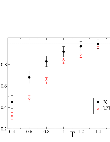
Figure 7.8: The violation factor $X=T/\Theta_{eff}$ that enters Eq. (7.80) (full circles) and the ratio $T/T_{eff}$ from the generalized FDR (open diamonds) as a function of the bath temperature $T$ for $\gamma=0.03$.

To test the conjecture of Bonetto and Gallavotti, see [129] and section 5.7, the Lyapunov spectra have been computed, see section 5.5. They are reported in Fig. 7.9 for $\gamma=0.03$, $T=1.2>T_{g}$ and $T=0.8<T_{g}$. Unfortunately, no qualitative change in the spectrum is observed on crossing $T_{g}$ and in particular no pairs of negative exponents are present above and below $T_{g}$. Thus, it seems that the theory of [129] does not apply to the model considered here below $T_{g}$. Note however that this theory is developed under the assumption of a strong chaoticity of the system, while below $T_{g}$ and for $\gamma\sim 0$ the dynamics of the system becomes slower and slower. Thus, the results presented here should not be regarded as invalidating the conjecture of [129], but as indicating that the hypothesis of [129] (essentially, the requirement of strong chaoticity) are not fulfilled by our model below $T_{g}$. This point requires further investigation.

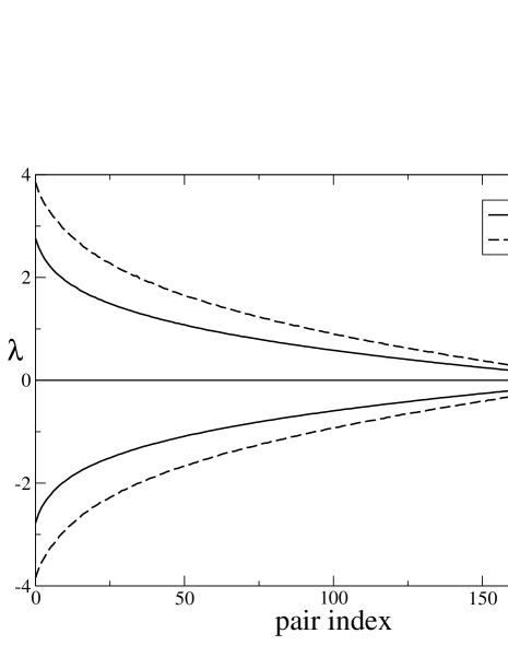
Figure 7.9: Lyapunov exponents for $\gamma=0.03$ and $T=0.8,1.2$. For both temperatures each pair consists of one positive and one negative exponent.

7.9 Discussion

An extension of the fluctuation theorem of Gallavotti and Cohen to open stochastic systems that are not able to equilibrate with their environments when relaxing unperturbed has been discussed.

The simplest example at hand has been used to test several generalized fluctuation formulas: a Brownian particle in a confining potential coupled to non-trivial external baths with different time-scales and temperatures. Independently of the form of the potential energies, due to the coupling to the complex environment, the particle is not able to equilibrate. Its relaxational dynamics is characterized by an effective temperature, defined via the modification of the fluctuation-dissipation relation between spontaneous and induced fluctuations. When no separation of time-scales can be identified in the bath, the effective temperature is a non-trivial function of the two times involved. Instead, when the bath evolves in different time-scales each characterized by a value of a temperature, the two-time dependent effective temperature is a piece-wise function that actually takes only these values, each one characterizing the dynamics of the particle in a regime of times.

The fluctuations of entropy production in a numerical simulation of a Lennard-Jones like fluid above and below the glass transition temperature $T_{g}$ have also been studied, obtaining results that partially confirm the theoretical analysis. However, many points are still open and require a much deeper numerical investigation.

Several authors discussed the possibility of introducing the effective temperature in the fluctuation theorem to extend its domain of applicability to glassy models driven by external forces [157, 159, 158, 160]. After summarizing the results of this chapter, it will be discussed how they compare to the proposals and findings presented here.

7.9.1 Summary of results

Different definitions of entropy production rate that are not equivalent when the effective temperature is not trivially equal to the ambient temperature have been discussed. It was found that:

1. The pdf of $\sigma^{\Theta}_{t}=W_{t}/\Theta$, where $W_{t}$ is the power dissipated by the external force and $\Theta$ is a free parameter with the dimensions of a temperature, does not satisfy the fluctuation theorem in general.

   The large deviation function, $\zeta_{\Theta}(p)$, still shows some interesting features revealing the existence of an effective temperature. When the bath has, say, two components acting on different time scales and with different temperatures, the function $[\zeta_{\Theta}(p)-\zeta_{\Theta}(-p)]/\sigma^{\Theta}_{+}$ may have different slopes corresponding to these two temperatures, one at small $p$ and the other at large $p$. The separation of time-scales of the bath translates into a separation of scales in the function $[\zeta_{\Theta}(p)-\zeta_{\Theta}(-p)]/\sigma^{\Theta}_{+}$.

   When the time scales of the baths are not separated, and one observes the large deviation function for not too large values of $p$ only, the fluctuation theorem is verified approximately if $\Theta$ is suitably chosen. Note that the temperature $\Theta_{eff}$ defined in this way is not equal to the effective temperature $T_{eff}$ that enters the modified fluctuation–dissipation relation in this case.

   Instead, when the time-scales are well separated, the two scales in the large deviation function are clearly visible and a single fitting parameter is not sufficient to make the fluctuation theorem hold.

2. The pdf of $\sigma^{eff}_{t}$ defined substituting the frequency dependent effective temperature to the constant $\Theta$ in the previous definition:

   $$\sigma^{eff}_{\tau}=\frac{\Delta\omega}{2\pi}\sum_{n=-\infty}^{\infty}\frac{-i\omega_{n}r_{\alpha}(\omega_{n})h_{\alpha}(\omega_{n})}{T_{eff}(\omega_{n})}=\int_{-\tau/2}^{\tau/2}dt\int_{-\tau/2}^{\tau/2}dt^{\prime}\,T^{-1}(t-t^{\prime})\dot{r}_{\alpha}(t)h_{\alpha}[\vec{r}(t^{\prime})]\ ,$$ (7.84)

   with $T^{-1}(t)$ the Fourier transform of $1/T_{eff}(\omega)$, the effective temperature of the relaxing system, see Eq. (6.42), always verifies the fluctuation theorem, as was shown analytically for the harmonic potential and numerically for the quartic one. No requirements on the characteristics of the bath are needed. $\sigma^{eff}_{t}$ reduces to $\sigma^{\Theta}_{t}$ when there is only one equilibrated bath.

3. The additional term $\sigma^{V}_{t}$ which is obtained from the Lebowitz–Spohn procedure, see equation (7.14), is not relevant for the applications discussed in this chapter, as it vanishes identically for harmonic potentials and for any potential in the adiabatic approximation. However it is relevant when the potential is nonlinear and the time scales are not separated. Its detailed investigation is left for future work.

4. If two time scales are present in the dynamics of a system and if the applied perturbation is periodic with frequency $\Omega<1/\tau_{s}$, $\tau_{s}$ being the largest relaxation time, the pdf of the power dissipated over a (large) number of cycles verifies the fluctuation relation with temperature $T_{s}=T_{eff}(\Omega)$. This is probably the easiest way of detecting the effective temperature by mean of the fluctuation relation.

5. These results should apply to driven glassy systems as discussed in section 7.5. It was shown, in a numerical simulation of a binary Lennard–Jones mixture, that below $T_{g}$ the Fluctuation Relation does not hold for $\sigma^{\Theta}$; the data –obtained in a situation where the time scales are not well separated– are consistent with the statements of item 1. above. The conjecture of Bonetto and Gallavotti that relates the factor $X$ in Eq. (7.80) to properties of the phase space of the considered system was tested; unfortunately, the data are not consistent with this conjecture, suggesting that the violation of the FR is, in the case studied above, of different origin than that proposed in [129]. This point also requires additional investigation.

Models like the one discussed here have been recently investigated [139, 161, 162, 163] to describe the dynamics of Brownian particles in complex media such as glasses, granular matter, etc. Brownian particles are often used as probes in order to study the properties of the medium (e.g. in Dynamic Light Scattering or Diffusing Wave Spectroscopy experiments). Moreover, confining potentials for Brownian particles can be generated using laser beams [167] and experiments on the fluctuations of the power dissipated in such systems are currently being performed [161, 168].

7.9.2 Effective temperatures

It is important to summarize the different definitions of effective temperature considered above and the relations between them. The effective temperature in the frequency domain is defined by equation (6.42) as a property of the bath which can also be measured from the ratio between correlation and response functions in the frequency domain. As discussed above, the same effective temperature enters the correct definition of entropy production rate in the frequency domain, see equation (7.84). Thus, experiments working in the frequency domain should observe the same effective temperature from the fluctuation–dissipation relation and from the fluctuation relation.

In the time domain the situation is slightly more complicated. On one hand, the effective temperature obtained from the fluctuation–dissipation relation in the time domain, defined for example by equation (6.50), is not the Fourier transform of $T_{eff}(\omega)$. A convolution with the correlation function is involved in the relation between $T_{eff}(\omega)$ and $T_{eff}(t)$. On the other hand, the effective temperature $T^{-1}(t)$ entering the entropy production is exactly the Fourier transform of $1/T_{eff}(\omega)$, see again equation (7.84). This can give rise to ambiguities when working in the time domain.

Most of these ambiguities disappear as long as the time scales in the problem are well separated. In this case, on each time scale a well defined effective temperature can be identified, and this temperature enters both the fluctuation–dissipation relation and the fluctuation relation: see e.g. the curve for $\tau=250$ in Fig. 7.3 and the expression of $\sigma^{eff}$ in the adiabatic approximation, equation (7.56). This is essentially related to the validity of the adiabatic approximation discussed in section 7.5.1.

The difference is relevant when the time scales of the two baths are not well separated, and a single effective temperature cannot be identified, see the curve for $\tau=1$ in Fig. 7.3. In this case, it was found that the fluctuation relation holds with –approximately– a single effective temperature $\Theta_{eff}$ but this temperature is not clearly related to the fluctuation–dissipation temperature in the time domain. This was also observed in numerical simulations on Lennard–Jones systems. Still, when moving to the frequency domain, the two effective temperatures should coincide.

Let us remark again that, when applying these results to real glassy systems in finite dimension, one should take care of the possibility that the effective temperature has large space fluctuations due to the heterogeneity of the dynamics [153, 154]. The extension of the results presented here to such a situation is left for future work.

7.9.3 Comparison with previous works

Several proposals to introduce the effective temperature into extensions of the fluctuation theorem appeared in the literature.

Sellitto studied the fluctuations of entropy production in a driven lattice gas with reversible kinetic constraints [157]. When coupling this system to an external particle reservoir with chemical potential $\mu$, a dynamic crossover from a fluid to a glassy phase is found around $\mu_{d}$. The glassy nonequilibrium phase is characterized by a violation of the fluctuation dissipation theorem in which the parametric relation between global integrated response and displacement yields a line with slope $\mu_{eff}$ [169].

One drives this (possibly already out of equilibrium) system by coupling two adjacent layers of the three dimensional periodic cube to particle reservoirs at different chemical potentials, $\mu_{+}$ and $\mu_{-}$. The former is allowed to assume values corresponding to the glassy phase, $\mu_{+}>\mu_{d}$, while $\mu_{-}$ is always below $\mu_{d}$. The results of the Montecarlo simulation are consistent with a generalized form of the fluctuation theorem:

$$\sigma_{\tau}=J_{\tau}(\mu_{eff}-\mu_{-})\;,$$ (7.85)

where $\sigma_{\tau}$ is the entropy production, $J_{\tau}$ is the particle current in the direction of the externally imposed chemical potential gradient averaged over a time-interval of duration $\tau$; $\mu_{eff}$ is an effective chemical potential and $\mu_{-}$ is the chemical potential of one of the layers. When the chemical potentials of the two reservoirs are in the fluid phase, $\mu_{eff}=\mu_{+}$ and the usual fluctuation relation holds. Instead, when $\mu_{+}$ is in the glassy phase, Sellitto found that Eq. (7.85) holds with $\mu_{eff}$ taking the value appearing in the violation of fluctuation-dissipation theorem in the aging regime of the undriven glassy system at $\mu_{+}$.

The formula (7.85) differs from the ones that were found to describe the oscillator problem in that in the case studied here, when translating from temperature to chemical potential, the full time-dependent $\mu(t)$ enters. Strictly, this improved definition should also apply to the lattice gas model. However in the case studied by Sellitto the fast dynamics is an “intra-cage” dynamics that likely does not contribute to the current. This is a case in which the perturbation does not produce dissipation at high frequency so that the difference arising from $\mu(t)\neq\mu_{eff}$ should be tiny in this case (see section 7.7).

More recently, Crisanti and Ritort [159] found that the probability distribution function of the fluctuations of heat exchanges, $Q$, between an aging random orthogonal model in its ‘activated regime’ (a long-time regime in which the energy-density decays as a logarithm of time) and the heat bath is rather well described by a stationary Gaussian part and a waiting-time dependent exponential tail towards small values of $Q$. Assuming that these events are of two types (‘stimulated’ and ‘spontaneous’) they proposed to fit the ratio between the pdf of positive and negative ‘spontaneous’ $Q$’s in the form of a fluctuation theorem, i.e. to be proportional to $e^{-2Q/\lambda}$, and relate $\lambda$ to the effective temperature of the fluctuation-dissipation relation. They found good agreement. Crisanti, Ritort and Picco are currently performing simulations to test this hypothesis in Lennard-Jones mixtures [170].

Another development is an attempt to generalize the situation considered by Crooks. He considered a problem that starts from equilibrium in zero field and evolves according to some stochastic dynamic rule in the presence of an arbitrary applied field [171] and found that the ratio between the probability of a trajectory and its time-reversed one is given by $e^{-\beta\int_{0}^{t_{max}}dth(t)\dot{O}(t)}$ with $h(t)$ the time-dependent external field that couples linearly to the observable $O$. For simplicity, one can focus on $O=\phi$ with $\phi$ a scalar field characterizing the system. In [158] the extension of this relation to the non-equilibrium ‘glassy’ case was conjectured. Separating the external fields $h$ and $\phi$ in their fast and slow components [172], $h=h_{f}+h_{s}$ and $\phi=\phi_{f}+\phi_{s}$, one then proposes that the pdfs of the trajectories of the slow components satisfy a relation similar to Crooks’ with the temperature replaced by the effective temperature (for a glassy non-equilibrium system with two correlation scales [140]).

Finally, it is worth to mention the work of Sasa [160] where he introduces an effective temperature in his definition of entropy production for the Kuramoto-Sivashinsky equation.

7.10 Appendix: Dirichlet boundary conditions for the white bath

A second possibility to calculate the functional integral in Eq. (7.21) is to impose Dirichlet boundary conditions $a(-\tau/2)=a(\tau/2)=0$. However, in this case it is possible to calculate $z(\lambda)$ only for $m=0$. The distribution of $a_{t}$ is obtained substituting $\rho_{\omega}=D(\omega)a_{\omega}$ in Eq. (7.25):

$$\begin{split}{\cal P}[a_{t}]&=\exp\left[-\frac{1}{2\gamma T}\int_{-\infty}^{\infty}\frac{d\omega}{2\pi}\ a_{\omega}|D(\omega)|^{2}\bar{a}_{\omega}\right]\\ &=\exp\left[-\frac{1}{2\gamma T}\int_{-\infty}^{\infty}dt\ a_{t}\left(k^{2}+\epsilon^{2}-2i\epsilon\gamma\frac{d}{dt}-\gamma^{2}\frac{d^{2}}{dt^{2}}\right)\bar{a}_{t}\right]\ .\end{split}$$ (7.86)

From Eq. (7.21)

$$\langle\exp[-\lambda\sigma_{\tau}]\rangle={\cal N}^{-1}\int da_{t}\exp\left[-\frac{1}{2\gamma T}\int_{-\infty}^{\infty}dt\ a_{t}\left(k^{2}+\epsilon^{2}-2i\epsilon\gamma[1-2\lambda\chi_{\tau}(t)]\frac{d}{dt}-\gamma^{2}\frac{d^{2}}{dt^{2}}\right)\bar{a}_{t}\right]\ ,$$ (7.87)

where $\chi_{\tau}(t)$ is the characteristic function of $t\in[-\tau/2,\tau/2]$. At the leading order in $\tau$, as the correlation function of $a_{t}$ decays exponentially on a time scale $\tau_{0}=\gamma k^{-1}$, one can integrate out the portion of the trajectory that is outside the interval $[-\tau/2,\tau/2]$ both in the numerator and the denominator, to obtain

$$\langle\exp[-\lambda\sigma_{\tau}]\rangle={\cal N}^{-1}\int da_{t}\exp\left[-\frac{1}{2\gamma T}\int_{-\tau/2}^{\tau/2}dt\ a_{t}\left(k^{2}+\epsilon^{2}-2i\epsilon\gamma(1-2\lambda)\frac{d}{dt}-\gamma^{2}\frac{d^{2}}{dt^{2}}\right)\bar{a}_{t}\right]\ .$$ (7.88)

Then one has to find the eigenvalues of the operator appearing in the integral. This corresponds to find the solution of the equation

$$J\bar{a}_{t}=\left(k^{2}+\epsilon^{2}-2i\epsilon\gamma(1-2\lambda)\frac{d}{dt}-\gamma^{2}\frac{d^{2}}{dt^{2}}\right)\bar{a}_{t}=E\bar{a}_{t}$$ (7.89)

with boundary conditions $\bar{a}(\tau/2)=\bar{a}(-\tau/2)=0$. Note that the operator $J$ is Hermitian, thus the eigenvalues are real; they are given by the following expression:

$$E_{n}(\lambda)=k^{2}+4\epsilon^{2}\lambda(1-\lambda)+\gamma^{2}\frac{\pi^{2}n^{2}}{\tau^{2}}$$ (7.90)

with $n=0,1,\cdots$. For each $n$ the integration is performed on one complex variable and one gets

$$\langle\exp[-\lambda\sigma_{\tau}]\rangle={\cal N}^{-1}\int da_{t}\exp\left[-\frac{1}{2\gamma T}\int_{-\tau/2}^{\tau/2}dt\ a_{t}J\bar{a}_{t}\right]=\prod_{n=0}^{\infty}\frac{E_{n}(0)}{E_{n}(\lambda)}$$ (7.91)

recalling that the constant ${\cal N}$ is simply the numerator calculated in $\lambda=0$. Finally one obtains, defining $\omega=n\pi/\tau$,

$$z(\lambda)=\lim_{\tau\rightarrow\infty}\frac{1}{\tau}\sum_{n=0}^{\infty}\log\frac{E_{n}(\lambda)}{E_{n}(0)}=\int_{0}^{\infty}\frac{d\omega}{\pi}\log\left[1+\frac{4\epsilon^{2}\lambda(1-\lambda)}{k^{2}+\gamma^{2}\omega^{2}}\right]$$ (7.92)

The latter expression verifies obviously the fluctuation theorem. Moreover, in the $m=0$ case Eq. (7.27) is equal to Eq. (7.92), as one can check using suitable changes of variable in the integral. In this simple case, $\zeta(p)$ can be computed exactly. Starting from Eq. (7.92) one has

$$z^{\prime}(\lambda)=\int_{0}^{\infty}\frac{d\omega}{\pi}\frac{4\epsilon^{2}(1-2\lambda)}{\gamma^{2}\omega^{2}+k^{2}+4\epsilon^{2}\lambda(1-\lambda)}=\frac{2\epsilon^{2}(1-2\lambda)}{\gamma\sqrt{k^{2}+4\epsilon^{2}\lambda(1-\lambda)}}\ ,$$ (7.93)

and, recalling that $z(0)=0$,

$$z(\lambda)=\int_{0}^{\lambda}d\mu\ z^{\prime}(\mu)=\gamma^{-1}\big{[}\sqrt{k^{2}+4\epsilon^{2}\lambda(1-\lambda)}-k\big{]}\ .$$ (7.94)

The function $\zeta(p)$ is defined by

$$\zeta(p)=\min_{\lambda}[\lambda p\sigma_{+}-z(\lambda)]=\lambda^{*}p\sigma_{+}-z(\lambda^{*})\ ,$$ (7.95)

where $\sigma_{+}=2\epsilon^{2}/(\gamma k)$ and $\lambda^{*}$ is defined by $z^{\prime}(\lambda^{*})=p\sigma_{+}$; hence,

$$p=\frac{k(1-2\lambda^{*})}{\sqrt{k^{2}+4\epsilon^{2}\lambda^{*}(1-\lambda^{*})}}\hskip 10.0pt\Rightarrow\hskip 10.0pt\lambda^{*}=\frac{1}{2}\left[1-p\sqrt{\frac{\epsilon^{2}+k^{2}}{\epsilon^{2}p^{2}+k^{2}}}\right]\ ,$$ (7.96)

and finally

$$\zeta(p)=\gamma^{-1}\left\{k+\frac{\epsilon^{2}p}{k}\left[1-p\sqrt{\frac{\epsilon^{2}+k^{2}}{\epsilon^{2}p^{2}+k^{2}}}\right]-k\sqrt{\frac{\epsilon^{2}+k^{2}}{\epsilon^{2}p^{2}+k^{2}}}\right\}\ .$$ (7.97)

From the latter expression it is easy to verify that

$$\zeta(p)-\zeta(-p)=\frac{2\epsilon^{2}p}{k}=p\sigma_{+}\ ,$$ (7.98)

as stated by the FT. Defining $\tau_{0}=\gamma/k$, the relaxation time of the correlation function of $a_{t}$, and $\sigma_{0}=\sigma_{+}\tau_{0}/2=\epsilon^{2}/k^{2}$, the (adimensional) entropy production over a time $\tau_{0}/2$, one obtains

$$\zeta(p)=\tau_{0}^{-1}\left[1+p\sigma_{0}-\sqrt{(1+\sigma_{0})(1+p^{2}\sigma_{0})}\right]\ .$$ (7.99)

7.11 Appendix: Fluctuation theorem for many equilibrium baths at different temperature

Here the function $z(\lambda)$ will be computed in the case in which the driven oscillator is coupled to $N$ colored baths with generic memory functions and in equilibrium at different temperatures. The violation of the fluctuation-dissipation theorem for the relaxing particle in such an environment was discussed in section 6.4.3. As discussed there, the equations are mathematically equivalent to the ones discussed in section 7.3.2; thus the strategy as well as many details of the calculation are the same as in sections 7.3.1 and 7.3.2.

The equations of motion are

$$m\ddot{a}_{t}+\sum_{i=1}^{N}\int_{-\infty}^{\infty}ds\ g_{i}(t-s)\dot{a}_{s}=-\kappa a_{t}+\sum_{i=1}^{N}\rho_{it}\ ,$$ (7.100)

with $\kappa=k-i\epsilon$. The thermal noises satisfy

$$\begin{split}&\langle\rho_{it}\rho_{j0}\rangle=\langle\bar{\rho}_{it}\bar{\rho}_{j0}\rangle=0\ ,\\ &\langle\rho_{it}\bar{\rho}_{j0}\rangle=\delta_{ij}T_{i}\nu_{i}(t)\ .\end{split}$$ (7.101)

By causality, the functions $g_{i}(t)$ must vanish for $t<0$. As the baths are in equilibrium at temperature $T_{i}$, the functions $\nu_{i}(t)$ and $g_{i}(t)$ are related by Eq. (6.43):

$$\begin{split}&\nu_{i}(t)=T_{i}[g_{i}(t)+g_{i}(-t)]=T_{i}g_{i}(|t|)\ ,\\ &T_{i}g_{i}(t)=\theta(t)\nu_{i}(t)\ .\end{split}$$ (7.102)

In the frequency domain Eq. (7.100) becomes

$$a_{\omega}=\frac{\sum_{i}\rho_{i\omega}}{-m\omega^{2}+\kappa-i\omega\sum_{i}g_{i}(\omega)}\equiv\frac{\sum_{i}\rho_{i\omega}}{D(\omega)}\ ,$$ (7.103)

where $D(\omega)=-m\omega^{2}+\kappa-i\omega\sum_{i}g_{i}(\omega)$.

The dissipated power is given by

$$\frac{dH}{dt}=2\epsilon\;{\rm Im}\,\dot{a}_{t}\bar{a}_{t}-2{\rm Re}\,\sum_{i}\int_{-\infty}^{\infty}ds\ g_{i}(t-s)\dot{a}_{t}\dot{\bar{a}}_{s}+2{\rm Re}\,\sum_{i}\dot{a}_{t}\bar{\rho}_{it}=W_{t}-\sum_{i}\widetilde{W}_{it}\;,$$ (7.104)

where as in the previous cases $W_{t}=2\epsilon{\rm Im}\,\dot{a}_{t}\bar{a}_{t}$ is the power injected by the external force and $\widetilde{W}_{it}=2{\rm Re}\,\int_{-\infty}^{\infty}ds\ g_{i}(t-s)\dot{a}_{t}\dot{\bar{z}}_{s}-2{\rm Re}\,\dot{a}_{t}\bar{\rho}_{it}$ is the power extracted by the $i$-th bath.

The first definition of entropy production rate, Eq. (7.34), gives (in the following, $\frac{\Delta\omega}{2\pi}\sum_{n=-\infty}^{\infty}\rightarrow\int_{-\infty}^{\infty}\frac{d\omega}{2\pi}$ as the error is $O(1)$ for $\tau\rightarrow\infty$, see section 7.3.1):

$$\sigma^{\Theta}_{\tau}=-\int_{-\infty}^{\infty}\frac{d\omega}{2\pi}\frac{2\epsilon\omega|a_{\omega}|^{2}}{\Theta}\ .$$ (7.105)

Substituting $a_{\omega}=\sum_{i}\rho_{i\omega}/D(\omega)$, one obtains

$$\langle\exp[-\lambda\sigma^{\Theta}_{\tau}]\rangle={\cal N}^{-1}\int d\rho_{i\omega}\ \exp\left[-\int_{-\infty}^{\infty}\frac{d\omega}{2\pi}\sum_{ij}\rho_{i\omega}A_{ij}^{\lambda}(\omega)\bar{\rho}_{j\omega}\right]\ ,$$ (7.106)

where $A^{\lambda}(\omega)$ is a $N\times N$ real matrix which elements are given by

$$A_{ij}^{\lambda}(\omega)=\frac{\delta_{ij}}{T_{i}\nu_{i}(\omega)}-\frac{\lambda}{|D(\omega)|^{2}}\frac{2\epsilon\omega}{\Theta}\ .$$ (7.107)

Then,

$$z_{\Theta}(\lambda)=\lim_{\tau\rightarrow\infty}\tau^{-1}\log\prod_{n=-\infty}^{\infty}\frac{\det A^{\lambda}(\omega_{n})}{\det A^{0}(\omega_{n})}=\int_{-\infty}^{\infty}\frac{d\omega}{2\pi}\ \log\left[\frac{\det A^{\lambda}(\omega)}{\det A^{0}(\omega)}\right]\ .$$ (7.108)

The determinant of a matrix of the form $A^{\lambda}_{ij}=c_{i}^{-1}\delta_{ij}+\lambda b$ satisfies the relation

$$\frac{\det A^{\lambda}}{\det A^{0}}=1+\lambda b\sum_{i}c_{i}\;;$$ (7.109)

one finally obtains

$$z_{\Theta}(\lambda)=\int_{-\infty}^{\infty}\frac{d\omega}{2\pi}\ \log\left[1-\frac{2\epsilon\lambda\omega\sum_{i}\frac{T_{i}}{\Theta}\nu_{i}(\omega)}{|D(\omega)|^{2}}\right]\ .$$ (7.110)

In general, it does not exist a choice of $\Theta$ such that $z_{\Theta}(\lambda)$ verifies the fluctuation theorem, i.e. $z_{\Theta}(\lambda)\neq z_{\Theta}(1-\lambda)$.

For the second definition, given by Eq. (7.33), the computation is identical to the one of the previous section with the substitution $\Theta\rightarrow T_{eff}(\omega)$, where $T_{eff}(\omega)$ is given by Eq. (6.49). The result is then

$$z_{eff}(\lambda)=\int_{-\infty}^{\infty}\frac{d\omega}{2\pi}\ \log\left[1-\frac{2\epsilon\lambda\omega\sum_{i}T_{i}\nu_{i}(\omega)}{T_{eff}(\omega)|D(\omega)|^{2}}\right]=\int_{-\infty}^{\infty}\frac{d\omega}{2\pi}\ \log\left[1-\frac{2\epsilon\lambda\omega\sum_{i}\nu_{i}(\omega)}{|D(\omega)|^{2}}\right]\ .$$ (7.111)

Observing that

$$\begin{split}&D(-\omega)=\overline{D(\omega)}-2i\epsilon\ ,\\ &|D(-\omega)|^{2}=|D(\omega)|^{2}-2\epsilon\omega\sum_{i}\nu_{i}(\omega)\ ,\end{split}$$ (7.112)

and using the same trick already used in section 7.3.1, it is easy to show that $z_{eff}(\lambda)=z_{eff}(1-\lambda)$.

7.12 Appendix: Entropy production of the thermal baths

A different definition of entropy production rate based on the power extracted by the thermal bath instead of the one injected by the driving force will be discussed in this section. The two differ by a total derivative if there is only one bath, see Eq. (7.18), so their asymptotic distributions should be identical at least for $|p|\leq 1$, see [120] and section 4.4.3.

If there are many baths equilibrated at different temperature, the study of the entropy production extracted by each bath allows to separate the different contributions to the total entropy production weighting each one with the right temperature, i.e. one can define the entropy production rate of the baths as

$$\sigma^{baths}_{t}=\sum_{i=1}^{N}\frac{\widetilde{W}_{it}}{T_{i}}\;.$$ (7.113)

This quantity takes into account heat exchanges between the baths, and its average value does not vanish at $\epsilon=0$, as will be shown in the following.

To compute $z_{baths}(\lambda)$, one rewrites Eq. (7.113) as:

$$\begin{split}\sigma^{baths}_{\tau}&=\int_{-\tau/2}^{\tau/2}dt\ \sigma^{baths}_{t}=\int_{-\infty}^{\infty}\frac{d\omega}{2\pi}{\rm Re}\,\sum_{i}\frac{2}{T_{i}}\Big{[}\omega^{2}|a_{\omega}|^{2}g_{i}(\omega)+i\omega a_{\omega}\bar{\rho}_{i\omega}\Big{]}\\ =&\int_{-\infty}^{\infty}\frac{d\omega}{2\pi}\left[\frac{\omega^{2}\big{|}\sum_{i}\rho_{i\omega}\big{|}^{2}\sum_{j}\frac{\nu_{j}(\omega)}{T_{j}}}{|D(\omega)|^{2}}+\sum_{ij}\rho_{i\omega}\bar{\rho}_{j\omega}\left(\frac{i\omega}{D(\omega)T_{j}}-\frac{i\omega}{\overline{D(\omega)}T_{i}}\right)\right]\ .\end{split}$$ (7.114)

Defining the functions

$$\begin{split}&p(\omega)=i\omega\overline{D(\omega)}\ ,\\ &F(\omega)=\omega^{2}\sum_{i}\frac{\nu_{i}(\omega)}{T_{i}}\ ,\end{split}$$ (7.115)

one obtains

$$\langle\exp[-\lambda\sigma^{baths}_{\tau}]\rangle={\cal N}^{-1}\int d\rho_{i\omega}\ \exp\left[-\int_{-\infty}^{\infty}\frac{d\omega}{2\pi}\sum_{ij}\rho_{i\omega}A_{ij}^{\lambda}(\omega)\bar{\rho}_{j\omega}\right]\ ,$$ (7.116)

where $A^{\lambda}(\omega)$ is a $N\times N$ matrix which elements are given by

$$A_{ij}^{\lambda}(\omega)=\overline{A_{ji}^{\lambda}(\omega)}=\frac{\delta_{ij}}{T_{i}\nu_{i}(\omega)}+\frac{\lambda}{|D(\omega)|^{2}}\left[F(\omega)+\frac{p(\omega)}{T_{j}}+\frac{\overline{p(\omega)}}{T_{i}}\right]\ .$$ (7.117)

Then,

$$z_{baths}(\lambda)=\lim_{\tau\rightarrow\infty}\tau^{-1}\log\prod_{n=-\infty}^{\infty}\frac{\det A^{\lambda}(\omega_{n})}{\det A^{0}(\omega_{n})}=\int_{-\infty}^{\infty}\frac{d\omega}{2\pi}\ \log\left[\frac{\det A^{\lambda}(\omega)}{\det A^{0}(\omega)}\right]\ .$$ (7.118)

The matrix $A$ has the following form:

$$A\sim\left(\begin{matrix}c_{i}^{-1}+\mu b_{ii}&\cdots&\mu b_{ij}\\ \vdots&\ddots&\vdots\\ \mu b_{ji}&\cdots&c_{j}^{-1}+\mu b_{jj}\end{matrix}\right)\ ,$$ (7.119)

where $\mu=\lambda/|D(\omega)|^{2}$, $c_{i}=T_{i}\nu_{i}(\omega)$ and $b_{ij}=F(\omega)+\frac{p(\omega)}{T_{j}}+\frac{\overline{p(\omega)}}{T_{i}}$. Its determinant is an order $N$ polynomial in $\mu$ of the following form:

$$\frac{\det A^{\lambda}}{\det A^{0}}=1+\mu\sum_{i}c_{i}b_{ii}+\mu^{2}\sum_{i<j}c_{i}c_{j}\left|\begin{matrix}b_{ii}&b_{ij}\\ b_{ji}&b_{jj}\end{matrix}\right|+\mu^{3}\sum_{i<j<k}c_{i}c_{j}c_{k}\left|\begin{matrix}b_{ii}&b_{ij}&b_{ik}\\ b_{ji}&b_{jj}&b_{jk}\\ b_{ki}&b_{kj}&b_{kk}\end{matrix}\right|+\cdots\ .$$ (7.120)

To compute the coefficients explicitly, define first $T_{ij}$ by $T_{ij}^{-1}=T_{i}^{-1}-T_{j}^{-1}$. The coefficient of $\lambda^{2}$ is given by a sum of determinants of the form

$$\left|\begin{matrix}F+\frac{p}{T_{i}}+\frac{\overline{p}}{T_{i}}&F+\frac{p}{T_{i}}+\frac{\overline{p}}{T_{j}}\\ F+\frac{p}{T_{j}}+\frac{\overline{p}}{T_{i}}&F+\frac{p}{T_{j}}+\frac{\overline{p}}{T_{j}}\end{matrix}\right|=\left|\begin{matrix}F+\frac{p}{T_{i}}+\frac{\overline{p}}{T_{j}}&\frac{\overline{p}}{T_{ji}}\\ F+\frac{p}{T_{j}}+\frac{\overline{p}}{T_{i}}&\frac{\overline{p}}{T_{ji}}\end{matrix}\right|=\left|\begin{matrix}\frac{p}{T_{ij}}&0\\ F+\frac{p}{T_{j}}+\frac{\overline{p}}{T_{i}}&\frac{\overline{p}}{T_{ji}}\end{matrix}\right|=-\frac{|p|^{2}}{\big{(}T_{ij}\big{)}^{2}}\ ,$$ (7.121)

where the first column was first subtracted from the second column, and then the second row was subtracted from the first row. All the coefficients of the higher powers of $\lambda$ vanish. Consider for example the coefficient of $\lambda^{3}$. It has the form

$$\begin{split}&\left|\begin{matrix}F+\frac{p}{T_{i}}+\frac{\overline{p}}{T_{i}}&F+\frac{p}{T_{i}}+\frac{\overline{p}}{T_{j}}&F+\frac{p}{T_{i}}+\frac{\overline{p}}{T_{k}}\\ F+\frac{p}{T_{j}}+\frac{\overline{p}}{T_{i}}&F+\frac{p}{T_{j}}+\frac{\overline{p}}{T_{j}}&F+\frac{p}{T_{j}}+\frac{\overline{p}}{T_{k}}\\ F+\frac{p}{T_{k}}+\frac{\overline{p}}{T_{i}}&F+\frac{p}{T_{k}}+\frac{\overline{p}}{T_{j}}&F+\frac{p}{T_{k}}+\frac{\overline{p}}{T_{k}}\end{matrix}\right|=\\ &\left|\begin{matrix}F+\frac{p}{T_{i}}+\frac{\overline{p}}{T_{i}}&\frac{\overline{p}}{T_{ji}}&\frac{\overline{p}}{T_{ki}}\\ F+\frac{p}{T_{j}}+\frac{\overline{p}}{T_{i}}&\frac{\overline{p}}{T_{ji}}&\frac{\overline{p}}{T_{ki}}\\ F+\frac{p}{T_{k}}+\frac{\overline{p}}{T_{i}}&\frac{\overline{p}}{T_{ji}}&\frac{\overline{p}}{T_{ki}}\end{matrix}\right|=\left|\begin{matrix}\frac{p}{T_{ik}}&0&0\\ \frac{p}{T_{jk}}&0&0\\ F+\frac{p}{T_{k}}+\frac{\overline{p}}{T_{i}}&\frac{\overline{p}}{T_{ji}}&\frac{\overline{p}}{T_{ki}}\end{matrix}\right|=0\ ,\end{split}$$ (7.122)

subtracting the first column to the second and third column, and then the third row to the first and second row. The same argument applies to all the other coefficients up to order $N$. Finally, one gets

$$\begin{split}\frac{\det A^{\lambda}(\omega)}{\det A^{0}(\omega)}&=1+\frac{\lambda}{|D(\omega)|^{2}}\sum_{i}T_{i}\nu_{i}(\omega)\left[F(\omega)+\frac{p(\omega)}{T_{i}}+\frac{\overline{p(\omega)}}{T_{i}}\right]-\frac{\lambda^{2}|p(\omega)|^{2}}{|D(\omega)|^{4}}\sum_{i<j}\frac{T_{i}T_{j}\nu_{i}(\omega)\nu_{j}(\omega)}{\big{(}T_{ij}\big{)}^{2}}\\ &=1-\frac{2\epsilon\omega\lambda\sum_{i}\nu_{i}(\omega)}{|D(\omega)|^{2}}+\frac{\lambda(1-\lambda)}{|D(\omega)|^{2}}\sum_{i<j}\frac{T_{i}T_{j}\nu_{i}(\omega)\nu_{j}(\omega)}{\big{(}T_{ij}\big{)}^{2}}\ ,\end{split}$$ (7.123)

and

$$z_{baths}(\lambda)=\int_{-\infty}^{\infty}\frac{d\omega}{2\pi}\log\left[1-\frac{2\epsilon\omega\lambda\sum_{i}\nu_{i}(\omega)}{|D(\omega)|^{2}}+\frac{\lambda(1-\lambda)}{|D(\omega)|^{2}}\sum_{i<j}\frac{T_{i}T_{j}\nu_{i}(\omega)\nu_{j}(\omega)}{\big{(}T_{ij}\big{)}^{2}}\right]\ .$$ (7.124)

The first term in the logarithm is proportional to $\epsilon$ and is related to the power injected by the external force, while the second term accounts for heat exchanges between the baths and does not vanish at $\epsilon=0$. Finally, observing that

$$\begin{split}&D(-\omega)=\overline{D(\omega)}-2i\epsilon\ ,\\ &|D(-\omega)|^{2}=|D(\omega)|^{2}-2\epsilon\omega\sum_{i}\nu_{i}(\omega)\ ,\end{split}$$ (7.125)

and using the same trick already used in section 7.3.1, it is easy to show that $z_{baths}(\lambda)=z_{baths}(1-\lambda)$. Thus $\zeta_{baths}(p)$ should verify the fluctuation relation at least for $|p|\leq 1$, if the contribution of boundary terms is not negligible. This result is of interest for the study of heat conduction and is similar to the one discussed in [84].

7.13 Appendix: Fluctuation relation for the spherical $p$-spin model

It has been shown in section 7.5 that the dynamics of the mean field spherical model is described by the following equation:

$$\begin{split}&\dot{\sigma}(t)=-\mu\sigma(t)+\int_{-\infty}^{\infty}dt^{\prime}\ \Sigma(t-t^{\prime})\sigma(t^{\prime})+\rho(t)+\epsilon h(t)\ ,\\ &\left\langle\rho(t)\rho(t^{\prime})\right\rangle=2T\delta(t-t^{\prime})+D_{0}(t-t^{\prime})\ ,\\ &\left\langle h(t)h(t^{\prime})\right\rangle=D_{1}(t-t^{\prime})\ ,\end{split}$$ (7.126)

where $\rho(t)$ and $h(t)$ are two uncorrelated Gaussian variables, and $\Sigma$, $D_{0}$ represent a nonequilibrium bath once the self-consistency equations for $R$ and $C$ are solved. The term $\epsilon h(t)$ represent the external drive.

This equation is a particular instance of the general equation

$$\begin{split}&m\ddot{x}(t)+\int_{-\infty}^{\infty}dt^{\prime}\,g(t-t^{\prime})\dot{x}(t^{\prime})=-kx(t)+\rho(t)+\epsilon h(t)\ ,\\ &\left\langle\rho(t)\rho(t^{\prime})\right\rangle=\nu(t-t^{\prime})\ ,\\ &\left\langle h(t)h(t^{\prime})\right\rangle=\mu(t-t^{\prime})\ ,\end{split}$$ (7.127)

with $m=0$, $\nu(\omega)=2T+D_{0}(\omega)$ and $g(\omega)=1+\Sigma(\omega)/(i\omega)$. This gives, in absence of drive, an effective temperature

$$T_{eff}(\omega)=\frac{\nu(\omega)}{2{\rm Re}\,g(\omega)}=\frac{2T+D_{0}(\omega)}{2{\rm Re}\,[1+\Sigma(\omega)/(i\omega)]}\ .$$ (7.128)

If $R$ and $C$ are related by the FDR, $R(t)=-\beta\theta(t)\dot{C}(t)$, from the relation $\Sigma=RD_{0}^{\prime}(C)$ follows that $\Sigma(t)=-\beta\theta(t)\dot{D}_{0}(t)$, i.e. $D_{0}(\omega)=2T{\rm Re}\,[\Sigma(\omega)/(i\omega)]$, see section 6.4.1, so $T_{eff}(\omega)\equiv T$ and the bath is in equilibrium, as expected. If $R$ and $C$ do not verify the FDR, $T_{eff}\neq T$.

The dissipated power is $W(t)=\epsilon h(t)\dot{x}(t)$, and its average is $\left\langle W(t)\right\rangle=\epsilon\left\langle h(t)\dot{x}(t)\right\rangle$. The linear equation (7.127) is solved by

$$x(t)=\int_{-\infty}^{\infty}dt^{\prime}\,R(t-t^{\prime})\big{[}\rho(t^{\prime})+\epsilon h(t^{\prime})\big{]}\ ,$$ (7.129)

so that

$$\left\langle W(t)\right\rangle=\epsilon\left\langle h(t)\dot{x}(t)\right\rangle=\epsilon\left\langle h(t)\int_{-\infty}^{\infty}dt^{\prime}\,\dot{R}(t-t^{\prime})\big{[}\rho(t^{\prime})+\epsilon h(t^{\prime})\big{]}\right\rangle=\epsilon^{2}\int_{-\infty}^{\infty}dt^{\prime}\,\dot{R}(t-t^{\prime})\mu(t-t^{\prime})\ ,$$ (7.130)

which gives Eq. (7.48).

Finally, it is possible to prove that the pdf of

$$\sigma^{eff}(t)=\epsilon\int_{-\infty}^{t}dt^{\prime}\,T^{-1}(t-t^{\prime})\big{[}h(t)\dot{x}(t^{\prime})+h(t^{\prime})\dot{x}(t)\big{]}$$ (7.131)

verifies the fluctuation relation. Following the strategy of section 7.3.1 and 7.3.2 one first rewrites

$$\sigma^{eff}_{\tau}=\epsilon\frac{\Delta\omega}{2\pi}\sum_{n=-\infty}^{\infty}\frac{h_{n}i\omega_{n}\bar{x}_{n}}{T_{eff}(\omega_{n})}\ ,$$ (7.132)

and then, using $x(\omega)=[\rho(\omega)+\epsilon h(\omega)]/D(\omega)$, with $D(\omega)=-m\omega^{2}-i\omega g(\omega)+k$, computes

$$\begin{split}\left\langle e^{-\lambda\sigma^{eff}_{\tau}}\right\rangle&={\cal N}^{-1}\int d\rho_{n}dh_{n}\exp\left[-\frac{\Delta\omega}{2\pi}\sum_{n=-\infty}^{\infty}\left(\frac{|\rho_{n}|^{2}}{2\nu(\omega_{n})}+\frac{|h_{n}|^{2}}{2\mu(\omega_{n})}+\lambda\epsilon\frac{h_{n}i\omega_{n}(\bar{\rho}_{n}+\epsilon\bar{h}_{n})}{T_{eff}(\omega_{n})\overline{D(\omega_{n})}}\right)\right]\\ &=\prod_{n=-\infty}^{\infty}\left[1+2\epsilon^{2}\lambda\frac{\mu(\omega)\omega^{2}{\rm Re}\,g(\omega)}{T_{eff}(\omega)|D(\omega)|^{2}}-\epsilon^{2}\lambda^{2}\frac{\mu(\omega)\nu(\omega)\omega^{2}}{[T_{eff}(\omega)]^{2}|D(\omega)|^{2}}\right]^{-\frac{1}{2}}\ ,\end{split}$$ (7.133)

so that, substituting Eq. (7.128),

$$z_{eff}(\lambda)=\frac{1}{2}\int_{-\infty}^{\infty}\frac{d\omega}{2\pi}\log\left[1+4\epsilon^{2}\lambda(1-\lambda)\frac{\mu(\omega)\omega^{2}[{\rm Re}\,g(\omega)]^{2}}{\nu(\omega)|D(\omega)|^{2}}\right]\ ,$$ (7.134)

which clearly verifies $z_{eff}(\lambda)=z_{eff}(1-\lambda)$.

7.14 Appendix: Correlation functions of the harmonic oscillator coupled to two baths

In the harmonic case, ${\cal V}(|a|^{2})=\frac{k}{2}|a|^{2}$, the correlation function of a variable $a_{t}$, whose time evolution is given by Eq. (7.40), can be computed analytically [139]. In the frequency domain, Eq. (7.40) reads:

$$a_{\omega}=\frac{\rho^{f}_{\omega}+\rho^{s}_{\omega}}{\kappa-i\omega\gamma_{f}-\frac{i\omega\gamma_{s}}{1-i\omega\tau_{s}}}\equiv\frac{\rho^{f}_{\omega}+\rho^{s}_{\omega}}{D(\omega)}\ ,$$ (7.135)

where $D(\omega)=\kappa-i\omega\gamma_{f}-\frac{i\omega\gamma_{s}}{1-i\omega\tau_{s}}$. Recalling that $\langle\rho^{f}_{\omega}\rho^{f}_{\omega^{\prime}}\rangle=4\pi\gamma_{f}T_{f}\delta(\omega+\omega^{\prime})$ and $\langle\rho^{s}_{\omega}\rho^{s}_{\omega^{\prime}}\rangle=\frac{4\pi\gamma_{s}T_{s}}{1+\omega^{2}\tau_{s}^{2}}\delta(\omega+\omega^{\prime})$, and defining $C(\omega)$ from $\langle a_{\omega}a_{\omega}^{\prime}\rangle=2\pi\delta(\omega+\omega^{\prime})C(\omega)$ one gets

$$\begin{split}&R(\omega)=\frac{da_{\omega}}{d\rho^{f}_{\omega}}=\frac{1}{D(\omega)}\ ,\\ &C(\omega)=\frac{2\gamma_{f}T_{f}+\frac{2\gamma_{s}T_{s}}{1+\omega^{2}\tau_{s}^{2}}}{\left|D(\omega)\right|^{2}}\ .\end{split}$$ (7.136)

The function $(1-\omega\tau_{s})D(\omega)$ is a polynomial in $\omega$ and its zeros are given by $\omega=-i\gamma_{\pm}$ where

$$\gamma_{\pm}=\frac{1}{2\gamma_{f}\tau_{s}}\left[(\kappa\tau_{s}+\gamma_{f}+\gamma_{s})\pm\sqrt{(\kappa\tau_{s}+\gamma_{f}+\gamma_{s})^{2}-4\kappa\tau_{s}\gamma_{f}}\right]\ ,$$ (7.137)

and ${\rm Re}\,\gamma_{\pm}>0$. The response function is then given by

$$R(t)=\int_{-\infty}^{\infty}\frac{d\omega}{2\pi}e^{-i\omega t}\frac{1}{D(\omega)}=\frac{\theta(t)}{\gamma_{f}\tau_{s}}\left[\frac{1-\gamma_{+}\tau_{s}}{\gamma_{-}-\gamma_{+}}e^{-\gamma_{+}t}+\frac{1-\gamma_{-}\tau_{s}}{\gamma_{+}-\gamma_{-}}e^{-\gamma_{-}t}\right]\ ,$$ (7.138)

and the correlation function is given by

$$C(t)=\frac{1}{(\gamma_{f}\tau_{s})^{2}}\left[\frac{\gamma_{f}T_{f}(1-\gamma_{+}^{2}\tau_{s}^{2})+\gamma_{s}T_{s}}{(\gamma_{-}-\gamma_{+})(\bar{\gamma}_{-}+\gamma_{+}){\rm Re}\,\gamma_{+}}e^{-\gamma_{+}t}+\frac{\gamma_{f}T_{f}(1-\gamma_{-}^{2}\tau_{s}^{2})+\gamma_{s}T_{s}}{(\gamma_{+}-\gamma_{-})(\bar{\gamma}_{+}+\gamma_{-}){\rm Re}\,\gamma_{-}}e^{-\gamma_{-}t}\right]\ .$$ (7.139)

In the case $\epsilon=0$, and in the limit $\gamma_{f}\ll\gamma_{s}\ll k\tau_{s}$ where the time scales of the two baths are well separated, one obtains

$$\begin{split}&\gamma_{+}\sim\frac{k\tau_{s}+\gamma_{s}}{\gamma_{f}\tau_{s}}\ ,\\ &\gamma_{-}\sim\frac{1}{\tau_{s}}\left(1-\frac{\gamma_{s}}{\gamma_{s}+k\tau_{s}}\ ,\right)\end{split}$$ (7.140)

and

$$\begin{split}&C(t)=\frac{T_{s}\gamma_{s}\tau_{s}}{(k\tau_{s}+\gamma_{s})^{2}}e^{-t/\tau_{s}}+\frac{T_{f}\tau_{s}}{k\tau_{s}+\gamma_{f}}e^{-\frac{k\tau_{s}+\gamma_{s}}{\gamma_{f}\tau_{s}}t}\ ,\\ &R(t)=\theta(t)\left[\frac{\gamma_{s}}{(k\tau_{s}+\gamma_{s})^{2}}e^{-t/\tau_{s}}+\frac{1}{\gamma_{f}}e^{-\frac{k\tau_{s}+\gamma_{s}}{\gamma_{f}\tau_{s}}t}\right]\ .\end{split}$$ (7.141)

From the latter expressions it is easy to check that one has $R(t)\sim-\beta_{f}\theta(t)\dot{C}(t)$ for short times ($t\ll\tau_{s}$) and $R(t)\sim-\beta_{s}\theta(t)\dot{C}(t)$ for large times ($t\sim\tau_{s}$). The same behavior is found in the limit of small dissipation (small $\epsilon$), as one can check plotting the exact expression for the functions $R(t)$ and $C(t)$.

7.15 Appendix: The expression of $\sigma^{eff}$ in the adiabatic approximation

Starting from the expression (7.42) for $\sigma^{eff}_{t}$ and from Eq. (7.44), and remembering the convention $\int_{-\infty}^{t}ds\ \delta(t-s)=\theta(0)=1/2$, one has:

$$\int_{-\infty}^{t}dt^{\prime}\ \frac{\dot{a}_{t}\bar{a}_{t^{\prime}}}{T^{*}(t-t^{\prime})}=\frac{\dot{a}_{t}\bar{a}_{t}}{2T_{f}}+\frac{\gamma_{s}}{2\Omega T_{f}\gamma_{f}(\tau_{s})^{2}}\left(1-\frac{T_{s}}{T_{f}}\right)\int_{-\infty}^{t}dt^{\prime}\ e^{-\Omega(t-t^{\prime})}\dot{a}_{t}\bar{a}_{t^{\prime}}\ .$$ (7.142)

One can substitute $a_{t}=H_{t}+w_{t}$ and neglect all the terms proportional to $H_{t}w_{t}$: indeed, such terms vanish when $\sigma^{eff}_{t}$ is integrated over time intervals of the order of $\tau_{s}$, as, on such time scales, $\langle w_{t}\rangle=0$ while $H$ is constant. The first term gives then

$$\frac{\dot{a}_{t}\bar{a}_{t}}{2T_{f}}=\frac{\dot{H}_{t}\bar{H}_{t}+\dot{w}_{t}\bar{w}_{t}}{2T_{f}}\ .$$ (7.143)

In the second term, as $\Omega\sim 1/\tau_{s}$, one approximates $\int_{-\infty}^{t}dt^{\prime}\ e^{-\Omega(t-t^{\prime})}\bar{a}_{t^{\prime}}\sim H_{t}/\Omega$ to obtain

$$\frac{\gamma_{s}}{2\Omega^{2}T_{f}\gamma_{f}(\tau_{s})^{2}}\left(1-\frac{T_{s}}{T_{f}}\right)\dot{H}_{t}\bar{H}_{t}\sim\frac{1}{2T_{s}}\left(1-\frac{T_{s}}{T_{f}}\right)\dot{H}_{t}\bar{H}_{t}\ .$$ (7.144)

The (imaginary part of the) sum of these two terms times $4\epsilon$ gives Eq. (7.56).

Acknowledgments

I had the opportunity to work, during these three years of Ph.D., under the joint supervision of Giorgio Parisi and Giancarlo Ruocco: they gave me the possibility to approach the statistical mechanics of disordered systems from both the theoretical and experimental side. The interaction with them has been for me a continuous source of new ideas and of a deeper understanding of many aspects of physics. I wish to thank them for that and for their continuous support and encouragement.

Moreover, I benefited from the close collaboration with L. Angelani, F. Bonetto, and A. Giuliani, and with L. Cugliandolo, J. Kurchan, and G. Gallavotti, who supervised part of this work. Without them most of the results that have been presented here would not have been obtained.

Most of the work was done in the Physics department of the University of Rome “La Sapienza” where the presence of two research centers (INFM - CRS SMC and INFM - CRS Soft) dedicated to the physics of disordered systems created a very stimulating environment, where it is possible to find expert people in theoretical, computational and experimental physics. Among them, I wish to thank T. Castellani, A. Cavagna, C. Conti, C. De Michele, L. Leuzzi, E. Marinari, E. Pontecorvo, F. Ricci Tersenghi, F. Sciortino, T. Scopigno, P. Tartaglia, E. Zaccarelli, for many useful discussions that often motivated and improved a lot the work presented here. I wish to especially thank R. Di Leonardo, who was always a reference point for discussing experimental results, and with whom I shared many discussions on “philosophical” aspects of the physics of disordered systems as well as on practical problems. I wish also to thank D. Benedetti, M. Ortolani, S. Speziale for many useful discussions on subjects that were not directly related to my work: they were very useful to enlarge my interests and enter in contact with new interesting subjects of research.

During these three years I also spent time in some institutions that I wish to thank for their hospitality: in particular the École Normale Supérieure in Paris, the Centre de Physique des Houches, the International Center for Theoretical Physics (ICTP) in Trieste, the University of La Habana, Cuba, and the Spinoza Institut in Utrecht.

Last but not least, I wish to thank A. Degasperis who supervised my first teaching experience in the best possible way.

This work is dedicated to my father Carlo.

List of Figures

1. 1.1 Viscosity and relaxation time of many glass formers
2. 1.2 Configurational entropy of four different fragile glass formers
3. 1.3 Angell plot of the configurational entropy
4. 1.4 Evolution of the TAP states of the spherical $p$-spin model
5. 1.5 Qualitative behavior of the complexity
6. 1.6 The two-replica potential in the spherical $p$-spin model
7. 1.7 The function $q(\epsilon)$ in short range systems
8. 1.8 Instanton profile close to $T_{K}$
9. 2.1 The equilibrium complexity as a function of the packing fraction
10. 2.2 Phase diagram of the molecular liquid
11. 2.3 Entropy of the liquid and of the glass
12. 2.4 Reduced pressure of the liquid and the glass
13. 2.5 Cage radius of the liquid and the glass
14. 2.6 Complexity of the metastable states
15. 2.7 Comparison of the results for the equilibrium complexity
16. 2.8 Comparison of the equation of state with numerical data
17. 3.1 Correlation between $\alpha$ and the fragility from IXS
18. 3.2 Transition temperatures, fragility and volume of the states for the spherical $p$-spin
19. 3.3 Angell plot of the complexity for the spherical $p$-spin
20. 3.4 Transition temperatures, fragility and volume of the states for the Ising $p$-spin
21. 3.5 Correlation between fragility and $\alpha$ for $p$-spin models
22. 3.6 Correlation between fragility and number of states in $p$-spin models
23. 3.7 Sketch of the evolution with $p$ of the $p$-spin free energy landscape
24. 4.1 Pictorial representation of an Anosov system
25. 4.2 An example of the functions $\widetilde{\zeta}(a)$ and $\widetilde{\zeta}_{0}(a)$
26. 5.1 The function $\eta_{\tau}(p)$ for Model I at $E=5$
27. 5.2 Estimate of the function $\zeta_{\infty}(p)$ for Model I at $E=5$
28. 5.3 Quantitative estimates of the precision of the data analysis
29. 5.4 Mobility as a function of the driving force for Model I
30. 5.5 Lyapunov exponents for Model I
31. 5.6 Mobility as a function of $T$ and $E$ for Model II
32. 5.7 The function $\zeta_{\infty}(p)$ for Model II with $T=1.1$ and $E=3$
33. 6.1 Correlation functions for the driven $p$-spin model
34. 6.2 Relaxation time for the driven $p$-spin model
35. 6.3 “Phase diagram” of the driven $p$-spin model
36. 6.4 Effective temperature for the driven $p$-spin model
37. 6.5 Schematic “phase diagram” of realistic glassy models
38. 7.1 pdf of $\sigma^{eff}_{t}$ for the harmonic and anharmonic potentials
39. 7.2 pdf of $\sigma^{\Theta}_{t}$ for the harmonic and anharmonic potentials
40. 7.3 Autocorrelation functions and FDT plot for the harmonic oscillator
41. 7.4 Power spectrum of the entropy production rate for the harmonic oscillator
42. 7.5 Large deviation function $\zeta_{\Theta}(p)$ for the harmonic oscillator
43. 7.6 Viscosity of the Lennard–Jones binary mixture as a function of $T$
44. 7.7 The functions $\zeta(p)$ for the Lennard-Jones system at $T=1.4>T_{g}$ and $T=0.8<T_{g}$
45. 7.8 FR violation factor $X$ as a function of $T$
46. 7.9 Lyapunov exponents at $T=1.2>T_{g}$ and $T=0.8<T_{g}$

Bibliography

- [1] C. A. Angell, Science 267, 1924 (1995).
- [2] C. A. Angell, J. Res. NIST 102, 171 (1997).
- [3] L.-M. Martinez and C. A. Angell, Nature (London) 410, 663 (2001).
- [4] H. Vogel, Phys. Z. 22, 645 (1921); G. S. Fulcher, J. Am. Ceram. Soc. 8, 339 (1923); G. Tamman and W. Hesse, Z. Anorg. Allg. Chem. 156, 245 (1926).
- [5] C. A. Angell, J. Non-Cryst. Solids 73, 1 (1985).
- [6] R. Richert, C. A. Angell, J. Chem. Phys. 108, 9016 (1998).
- [7] W. Kauzmann, Chem. Rev. 43, 219 (1948).
- [8] A. Cavagna, I. Giardina and T. S. Grigera, J. Chem. Phys. 118, 6974 (2003); A. Cavagna, I. Giardina and T. S. Grigera, Europhys. Lett. 61, 74 (2003); A. Cavagna, A. Attanasi and J. Lorenzana, Phys. Rev. Lett. 95, 115702 (2005).
- [9] G. Adam and J. H. Gibbs, J. Chem. Phys. 43, 139 (1965).
- [10] T. R. Kirkpatrick and P. Wolynes, Phys. Rev. B 36, 8552 (1987); T. R. Kirkpatrick, D. Thirumalai and P. G. Wolynes, Phys. Rev. A 40, 1045 (1989).
- [11] P. G. Wolynes, Jour. Res. NIST, 102, 187 (1997).
- [12] X. Xia and P. G. Wolynes, Proc. Nat. Acad. Sci. 97, 2990 (2000); Phys. Rev. Lett 86, 5526 (2001).
- [13] V. Lubchenko and P. Wolynes, J. Chem. Phys 119, 9088 (2003).
- [14] J. P. Bouchaud and G. Biroli, J. Chem. Phys. 121, 7347 (2004).
- [15] M. Mézard and G. Parisi, J. Chem. Phys. 111, 1076 (1999).
- [16] T. Geszti, J. Phys. C 16, 5805 (1983); E. Leutheusser, Phys. Rev. A 29, 2765 (1984); U. Bendtzelius, W. Götze and A. Sjölander, J. Phys. C 17, 5915 (1984).
- [17] T. R. Kirkpatrick and P. G. Wolynes, Phys. Rev. A 35, 3072 (1987); T. R. Kirkpatrick and D. Thirumalai, Phys. Rev. Lett. 58, 2091 (1987).
- [18] D. J. Gross and M. Mézard, Nucl. Phys. B 240, 431 (1984).
- [19] H. Rieger, Phys. Rev. B 46, 14655 (1992).
- [20] J. Kurchan, G. Parisi and M. A. Virasoro, J. Phys. I (France) 3, 1819 (1993).
- [21] A. Crisanti and H. J. Sommers, Z. Phys. B 87, 341 (1992); A. Crisanti, H. Horner and H. J. Sommers, Z. Phys. B 92, 257 (1993).
- [22] A. Crisanti and H. J. Sommers, J. Phys. I (France) 5, 805 (1995).
- [23] A. Cavagna, I. Giardina and G. Parisi, J. Phys. A: Math. Gen. 30, 7021 (1997).
- [24] T. Castellani and A. Cavagna, J. Stat. Mech. (2005) P05012.
- [25] W. Götze and L. Sjögren, Phys. Rev. A 43, 5442 (1991).
- [26] W. van Megen and S. M. Underwood, Phys. Rev. Lett. 70, 2766 (1993).
- [27] J.-P. Bouchaud, L. Cugliandolo, J. Kurchan and M. Mézard, Out of equilibrium dynamics in spin-glasses and other glassy systems, in “Spin Glasses and Random Fields”, edited by A. P. Young (World Scientific, Singapore, 1998), cond-mat/9702070.
- [28] L. F. Cugliandolo, Dynamics of glassy systems, in “Slow relaxation and nonequilibrium dynamics in condensed matter”, Les Houches Session 77, J-L Barrat et al eds. (Springer-Verlag, Berlin, 2002), cond-mat/0210312.
- [29] M. Mézard, G. Parisi and M. A. Virasoro, Spin glass theory and beyond (World Scientific, Singapore, 1987).
- [30] G. Gallavotti, Statistical mechanics. A short treatise (Springer Verlag, Berlin, 1999).
- [31] D. J. Thouless, P. W. Anderson and R. G. Palmer, Phil. Mag. 35, 593 (1977).
- [32] A. Montanari and F. Ricci-Tersenghi, Eur. Phys. J. B 33, 339 (2003).
- [33] G. Ruocco and F. Sette, J. Phys.: Condens. Matter 13, 9141 (2001).
- [34] F. H. Stillinger and T. A. Weber, Phys. Rev. A 28, 2408 (1983); S. Sastry, J. Phys.: Condens. Matter, 12, 6515 (2000); S. Corezzi, L. Comez and D. Fioretto, Eur. Phys. J. E 14, 143 (2004); D. Prevosto, M. Lucchesi, S. Capaccioli, R. Casalini and P. A. Rolla, Phys. Rev. B 67, 174202 (2003).
- [35] S. Franz, G. Parisi and M. A. Virasoro, J. Phys. I France 2, 1869 (1992).
- [36] S. Franz and G. Parisi, J. Phys. I France 5, 1401 (1995).
- [37] R. Monasson, Phys. Rev. Lett. 75, 2847 (1995).
- [38] S. Franz and G. Parisi, Phys. Rev. Lett. 79, 2486 (1997).
- [39] A. Barrat, S. Franz and G. Parisi, J. Phys. A: Math. Gen. 30, 5593 (1997).
- [40] M. Mézard, Physica A 265, 352 (1999).
- [41] M. Mézard and G. Parisi, J. Phys.: Condens. Matter 12, 6655 (2000).
- [42] S. Franz, G. Parisi and M. A. Virasoro, cond-mat/9405007.
- [43] G. Parisi, cond-mat/9411115.
- [44] G. Parisi, G. Ruocco and F. Zamponi, Phys. Rev. E 69, 061505 (2004).
- [45] S. Franz and F. L. Toninelli, Phys. Rev. Lett. 92, 030602 (2004).
- [46] S. Franz, J. Stat. Mech. (2005) P04001.
- [47] M. Dzero, J. Schmalian and P. G. Wolynes, Phys. Rev. B 72, 100201 (2005).
- [48] M. D. Ediger, Ann. Rev. Phys. Chem. 51, 99 (2000).
- [49] B. Coluzzi, M. Mézard, G. Parisi and P. Verrocchio, J. Chem. Phys. 111, 9039 (1999).
- [50] L. Angelani, G. Foffi, F. Sciortino and P. Tartaglia, J. Phys.: Condens. Matter 17, L113 (2005).
- [51] S. N. Isakov, Comm. Math. Phys. 95, 427 (1984).
- [52] M. D. Rintoul and S. Torquato, J. Chem. Phys. 105, 9258 (1996).
- [53] M. Robles, M. López de Haro, A. Santos and S. Bravo Yuste, J. Chem. Phys. 108, 1290 (1998).
- [54] R. J. Speedy, Mol. Phys. 95, 169 (1998).
- [55] M. Tarzia, A. De Candia, A. Fierro, M. Nicodemi and A. Coniglio, Europhys. Lett. 66, 531 (2004).
- [56] F. Sciortino, W. Kob, P. Tartaglia, Phys. Rev. Lett. 83, 3214 (1999).
- [57] L. Angelani, G. Foffi and F. Sciortino, cond-mat/0506447.
- [58] M. Cardenas, S. Franz and G. Parisi, J. Phys. A 31, L163 (1998); J. Chem. Phys. 110, 1726 (1999).
- [59] J. G. Berryman, Phys. Rev. A 27, 1053 (1983).
- [60] G. D. Scott and D. M. Kilgour, Brit. J. Appl. Phys. (J. Phys. D) 2, 863 (1969).
- [61] J. L. Finney, Proc. R. Soc. London, Ser. A 319, 479 (1970).
- [62] C. H. Bennett, J. Appl. Phys. 43, 2727 (1972).
- [63] A. J. Matheson, J. Phys. C: Solid State Phys. 7, 2569 (1974).
- [64] M. J. Powell, Phys. Rev. B 20, 4194 (1979).
- [65] S. Alexander, Phys. Rep. 296, 65 (1998).
- [66] L. E. Silbert, D. E. Ertas, G. S. Grest, T. C. Halsey, and D. Levine, Phys. Rev. E 65, 031304 (2002).
- [67] M. Mézard and G. Parisi, Phys. Rev. Lett. 82, 747 (1999).
- [68] J.-P. Hansen and I.R. McDonald, Theory of simple liquids (Academic Press, London, 1986).
- [69] K. Ngai, J. Non Cryst. Solids, 275, 7 (2000).
- [70] A. P. Sokolov, E. Rössler, A. Kisliuk and D. Quitmann, Phys. Rev. Lett., 71, 2062 (1993); S. Yannopoulos and G. Papatheodorou, Phys. Rev. E 62, 3728 (2000).
- [71] R. Hall and P. Wolynes, J. Chem. Phys. 86, 2943 (1987); J. C. Dyre and N. B. Olsen, Phys. Rev. Lett. 91, 155703 (2003).
- [72] T. Scopigno, G. Ruocco, F. Sette and G. Monaco, Science 302, 849 (2003).
- [73] R. J. Speedy, J. Phys. Chem. B103, 4060 (1999).
- [74] S. Sastry, Nature (London) 409, 164 (2001).
- [75] P. G. Debenedetti and F. H. Stillinger, Nature (London) 410, 259 (2001).
- [76] G. Ruocco, F. Sciortino, F. Zamponi, T. Scopigno and C. De Michele, J. Chem. Phys. 120, 10666 (2004).
- [77] B. Derrida, Phys. Rev. Lett. 45, 79 (1980); Phys. Rev. B 24, 2613 (1981).
- [78] I. Saika-Voivod, P. H. Poole and F. Sciortino, Nature (London) 412, 514 (2001).
- [79] A. J. Moreno, S. V. Buldyrev, E. La Nave, I. Saika-Voivod, F. Sciortino, P. Tartaglia and E. Zaccarelli, Phys. Rev. Lett. 95, 157802 (2005).
- [80] D.J. Evans and G.P. Morris, Statistical Mechanics of Nonequilibrium Liquids (Academic Press, London, 1990).
- [81] D. Ruelle, Physics Today, May, 48 (2004).
- [82] S. de Groot and P. Mazur, Non equilibrium thermodynamics, Dover, 1984, (reprinted).
- [83] D. Ruelle, J. Stat. Phys. 85, 1 (1996).
- [84] G. Gallavotti, Chaos 14, 680 (2004).
- [85] Y. G. Sinai, Functional Analysis and Applications 2, n.1, 64 (1968); Functional Analysis and Applications 2, n.2, 70 (1968).
- [86] Y. G. Sinai, Russian Mathematical Surveys 166, 21 (1972).
- [87] Y. G. Sinai, Lectures in ergodic theory, Lecture notes in Mathematics (Princeton U. Press, Princeton, 1977).
- [88] D. Ruelle, Annals of the New York Academy of Sciences 356, 408 (1978).
- [89] D. Ruelle, Annals of the New York Academy of Sciences 357, 1 (1980).
- [90] G. Gallavotti, Fluid mechanics. Foundations (Springer-Verlag, Berlin, 2002).
- [91] G. Gallavotti, F. Bonetto, G. Gentile, Aspects of the ergodic, qualitative and statistical properties of motion (Springer Verlag, Berlin, 2004).
- [92] G. Gallavotti and E.G.D. Cohen, Phys. Rev. Lett. 74, 2694 (1995).
- [93] G. Gallavotti and E. G. D. Cohen, J. Stat. Phys. 80, 931 (1995).
- [94] D. J. Evans, E. G. D. Cohen and G. P. Morriss, Phys. Rev. Lett. 71, 2401 (1993).
- [95] F. Bonetto, G. Gallavotti and P. L. Garrido, Physica D 105, 226 (1997).
- [96] F. Bonetto, N. I. Chernov and J. L. Lebowitz, Chaos 8, 823 (1998).
- [97] L. Biferale, D. Pierotti and A. Vulpiani, J. Phys. A: Math. Gen. 31, 21 (1998).
- [98] G. Gallavotti and F. Perroni, chao-dyn/9909007.
- [99] L. Rondoni and E. Segre, Nonlinearity 12, 1471 (1999).
- [100] F. Zamponi, G. Ruocco and L. Angelani, J. Stat. Phys. 115, 1655 (2004).
- [101] G. Gallavotti, L. Rondoni and E. Segre, Physica D 187, 338 (2004).
- [102] A. Giuliani, F. Zamponi and G. Gallavotti, J. Stat. Phys. 119, 909 (2005).
- [103] S. Ciliberto and C. Laroche, J. Phys. IV 8, Pr6-215 (1998).
- [104] W. I. Goldburg, Y. Y. Goldschmidt and H. Kellay, Phys. Rev. Lett. 87, 245502 (2001).
- [105] S. Ciliberto, N. Garnier, S. Hernandez, C. Lacpatia, J.-F. Pinton and G. Ruiz Chavarria, Physica A 340, 240 (2004).
- [106] K. Feitosa and N. Menon, Phys. Rev. Lett. 92, 164301 (2004).
- [107] G. Gallavotti, Mathematical Physics Electronic Journal (MPEJ), 1, 1 (1995).
- [108] J. L. Lebowitz and H. Spohn, J. Stat. Phys. 95, 333 (1999).
- [109] G. Gallavotti, Phys. Rev. Lett. 77, 4334 (1996).
- [110] G. Gallavotti, J. Stat. Phys. 84, 899 (1996).
- [111] G. Gallavotti and D. Ruelle, Comm. Math. Phys. 190, 279 (1997).
- [112] G. Gallavotti, Open Systems and Information Dynamics 6, 101 (1999).
- [113] D. Ruelle, J. Stat. Phys. 95, 393 (1999).
- [114] D. Ruelle, J. Stat. Phys. 100, 757 (2000).
- [115] D. J. Evans and S. Sarman, Phys. Rev. E 48, 65 (1993).
- [116] D. J. Evans, Mol. Phys. 80, 221 (1993).
- [117] Z. S. She and E. Jackson, Phys. Rev. Lett. 70, 1255 (1993).
- [118] F. Bonetto, G. Gallavotti, A. Giuliani and F. Zamponi, cond-mat/0507672.
- [119] F. Bonetto, G. Gentile and V. Mastropietro, Ergodic Theory and Dynamical Systems 20, 681 (2000).
- [120] R. van Zon and E. G. D. Cohen, Phys. Rev. E 69, 056121 (2004).
- [121] C. Maes, J. Stat. Phys. 95, 367 (1999).
- [122] G. Gentile, Forum Mathematicum 10, 89 (1998).
- [123] L. Rondoni and G. P. Morriss, Open Systems and Information Dynamics 10, 105 (2003).
- [124] M. P. Allen and D. J. Tildesley, Computer simulation of liquids (Oxford Science Publications, 1987).
- [125] S. S. Sarman, D. J. Evans and P. T. Cummings, Phys. Rep. 305, 1 (1998).
- [126] W. Kob and C. H. Andersen, Phys. Rev. Lett. 73, 1376 (1994).
- [127] C. De Michele, F. Sciortino and A. Coniglio, J. Phys.: Condens. Matter 16, L489 (2004); L. Angelani, C. De Michele, G. Ruocco and F. Sciortino, J. Chem. Phys. 121, 7533 (2004).
- [128] G. Benettin, L. Galgani and J.-M. Strelcyn, Phys. Rev. A 14, 2338 (1976).
- [129] F. Bonetto and G. Gallavotti, Comm. Math. Phys. 189, 263 (1997).
- [130] D. J. Searles, D. J. Evans and D. J. Isbister, Chaos 8, 337 (1998).
- [131] C. P. Dettmann and G. P. Morriss, Phys. Rev. E 53, R5545 (1996).
- [132] M. Fisz, Probability theory and mathematical statistics (Wiley, New York, 1963).
- [133] G. Gallavotti, Comm. Math. Phys. 27, 103 (1972).
- [134] J. Kurchan, Comptes Rendus de l’Académie des Sciences, Series IV - Physics, 2, 239 (2001), cond-mat/0011110.
- [135] W. Götze, J. Phys.: Condens. Matter 11, A1 (1999).
- [136] H. Z. Cummins, J. Phys.: Condens. Matter 11, A95 (1999).
- [137] A. Crisanti and F. Ritort, J. Phys. A 36, R181 (2003).
- [138] L. F. Cugliandolo, J. Kurchan and L Peliti, Phys. Rev. E 55, 3898 (1997).
- [139] L. F. Cugliandolo and J. Kurchan, Frontiers in Magnetism, J. Phys. Soc. Japan Suppl. A 69, 247 (2000), cond-mat/9911086.
- [140] L. F. Cugliandolo and J. Kurchan, Phys. Rev. Lett. 71, 173 (1993).
- [141] L. F. Cugliandolo and J. Kurchan, J. Phys. A 27, 5749 (1994).
- [142] A. Cavagna, I. Giardina and G. Parisi, Phys. Rev. B 57, 11251 (1998); J. Phys. A 34, 5317 (2001).
- [143] A. Cavagna, I. Giardina and T. Grigera, J. Phys 36, 10721 (2003).
- [144] J.-P. Bouchaud, L. F. Cugliandolo, J. Kurchan and M. Mézard, Physica A 226, 243 (1996).
- [145] L. F. Cugliandolo, J. Kurchan, P. Le Doussal and L. Peliti, Phys. Rev. Lett. 78, 350 (1997).
- [146] L. Berthier, J.L. Barrat and J. Kurchan, Phys. Rev. E 61, 5464 (2000).
- [147] A. J. Liu and S. R. Nagel, Nature (London) 396, 21 (1998).
- [148] S. Fielding, P. Sollich and P. Mayer, J. Phys.: Conden. Matter 14, 1683-1696 (2002); P. Sollich, J. Phys. A 36, 10807-10818 (2003); E. Bertin, O. Dauchot and M. Droz, Phys. Rev. E 71, 046140 (2005).
- [149] G. Parisi, Phys. Rev. Lett. 79, 3660 (1997); J.-L. Barrat and W. Kob, Europhys. Lett. 46, 637 (1999); W. Kob and J.-L. Barrat, Eur. Phys. J. B 13, 319 (2000); R. di Leonardo, L. Angelani, G. Parisi and G. Ruocco, Phys. Rev. Lett. 84, 6054 (2000); F. Sciortino and P. Tartaglia, Phys. Rev. Lett. 86, 107 (2001).
- [150] J.L. Barrat and L. Berthier, Phys. Rev. E 63, 012503 (2000).
- [151] L. Berthier and J.L. Barrat, J. Chem. Phys. 116, 6228 (2002).
- [152] P. Le Doussal, L. F. Cugliandolo and L. Peliti, Europhys. Lett. 39, 111 (1997); A. Barrat, J. Kurchan, V. Loreto and M. Sellitto, Phys. Rev. Lett. 85, 5034 (2000); A. Kolton, R. Exartier, D. Domínguez, L. F. Cugliandolo and N. Gronbech-Jensen, Phys. Rev. Lett. 89, 227001 (2002); F. Corberi, G. Gonnella, E. Lippiello and M. Zannetti, J. Phys. A 36, 4729 (2003); F. Sastre, I. Dornic and H. Chaté, Phys. Rev. Lett. 91, 267205 (2003); K. Hayashi and S. Sasa, Phys. Rev. E 69, 066119 (2004); L. Arrachea and L. F. Cugliandolo, Europhys. Lett. 70, 642 (2005); T. Nakamura, M. Otsuki, S. Sasa, cond-mat/0410386.
- [153] H. Castillo, C. Chamon, L. F. Cugliandolo, J. L. Iguain and M. P. Kennett, Phys. Rev. B 68, 134442 (2003).
- [154] L. F. Cugliandolo, Heterogeneities and local fluctuations in glassy systems, SPIE, Vol. 5112, proceedings of ‘Noise as a tool for studying materials’, Symposium ‘Noise and Fluctuations’, ed. by M. B. Weissman, N. E. Israeloff, A. S. Kogan, (SPIE, Bellingham, WA, 2003), Santa Fe, New Mexico, USA, June 2003; cond-mat/0401506.
- [155] R. Di Leonardo, F. Ianni and G. Ruocco, Phys. Rev. E 71, 011505 (2005).
- [156] J. Kurchan, J. Phys. A 31, 3719 (1998).
- [157] M. Sellitto, cond-mat/9809186.
- [158] G. Semerjian, L. F. Cugliandolo and A. Montanari, J. Stat. Phys 115, 493 (2004).
- [159] A. Crisanti and F. Ritort, Europhys. Lett. 66, 253 (2004).
- [160] S. Sasa, nlin.CD/0010026.
- [161] B. Abou and F. Gallet, Phys. Rev. Lett. 93, 160603 (2004).
- [162] N. Pottier and A. Mauger, Physica A 332, 15 (2004).
- [163] N. Pottier, Physica A 345, 472 (2005).
- [164] F. Zamponi, G. Ruocco and L. Angelani, Phys.Rev.E 71, 020101(R) (2005).
- [165] G. Gallavotti, Physica A 263, 39 (1999).
- [166] L. Angelani, G. Ruocco, F. Sciortino, P. Tartaglia and F. Zamponi, Phys. Rev. E 66, 061505 (2002).
- [167] D. G. Grier, Nature (London) 424, 810 (2003).
- [168] G. M. Wang, E. M. Sevick, E. Mittag, D. J. Searles and D. J. Evans, Phys. Rev. Lett. 89, 050601 (2002).
- [169] J. Kurchan, L. Peliti and M. Sellitto, Europhys. Lett. 39, 365 (1997).
- [170] A. Crisanti, M. Picco and F. Ritort, in preparation.
- [171] G. E. Crooks, Phys. Rev. E 60, 2721 (1999); Phys. Rev. E 61, 2361 (2000).
- [172] S. Franz and M. A. Virasoro, J. Phys. A 33, 891 (2000); F. Corberi, E. Lippiello and M. Zannetti, Phys. Rev. E 65, 046136 (2002).