Phase transitions in one dimension: are they all driven by domain walls?

Abstract

Two known distinct examples of one-dimensional systems which are known to exhibit a phase transition are critically examined: (A) a lattice model with harmonic nearest-neighbor elastic interactions and an on-site Morse potential, and (B) the ferromagnetic, spin $1/2$ Ising model with long-range pair interactions varying as the inverse square of the distance between pairs. In both cases it can be shown that the domain wall configurations become entropically stable at, or very near, the critical temperature. This might provide a “positive” criterion for the occurrence of a phase transition in one-dimensional systems.

I Introduction

Phase transitions do not generally occur in one-dimensional systems. Their absence has been codified under a variety of conditions. Van Hove vanHove showed that, for particle systems with pair interactions of sufficiently short range, the free energy does not have any singularities. Landau Landau argued that a bistable system with finite interface energy will achieve an entropic gain by breaking up into a macroscopic number of domains, making macroscopic phase coexistence at any positive temperature impossible. His argument explains the absence of a phase transition in a large class of one-dimensional systems, which includes the short-range $S=1/2$ Ising model, the $\phi^{4}$ model, etc.

How does theory cope with the exceptions from the broad rule? Proofs of the van Hove type are in essence proofs of analyticity. In principle they can be extended, refined and thus provide sharper criteria for the absence of a phase transitionCuesta . Nonetheless, it is not straightforward to make a positive statement about a system where a phase transition actually occurs. On the other hand, Landau’s approach turns out to be more potent, because it can be “inverted” to describe the exact pathology which is necessary to produce macroscopic phase coexistence. Instead of setting out to prove that a finite interface energy will lead to a macroscopic number of domains because of the entropic gain invoved, it is possible to look at a single, possibly pathological interface, or domain wall (DW), and examine under which conditions the entropic gain might lead to its spontaneous formation. The question at hand is whether the conditions for spontaneous formation of a single interface are the same as those for a thermodynamic instability of the low-temperature phase, or, equivalently, for macroscopic phase coexistence. If the conditions are the same, i.e. if (i) spontaneous DW formation occurs at some temperature $T^{*}$, (ii) a macroscopic instability / phase transition is known by independent means to occur at a temperature $T_{c}$, and (iii) $T^{*}=T_{c}$, then it is not unreasonable to argue that the transition is driven by the formation of the DW.

In this paper I will review how this can be done in two representative cases: (A) models of one-dimensional thermodynamic instabilities (interfacial wetting, DNA denaturation), (B) the $S=1/2$ ferromagnetic Ising model with inverse-square interaction. Case (A) will be illustrated by the Peyrard-Bishop PB Hamiltonian (continuum and discrete) - although this should be regarded as representative of a much broader class of on-site potentials with a repulsive core, a stable minimum and a flat top. A proper understanding of how DW formation governs one-dimensional phase transitions includes a discussion of symmetric on-site potentials, where the pathology is “accidentally” lifted and a phase transition does not occur. In a sense this represents a special case of (A) and will be treated accordingly. Case (B) has been recognized for a long time as a key representative of marginal pathology; in particular, Thouless Thou69 has used a Landau-type of argument to predict the occurrence of long-range order at low temperatures; his argument however does not lead to an estimate of the critical temperature. It turns out that a “literal” application of the single-DW criterion (spontaneous DW formation), which has been successful in the case of thermodynamic instabilities, yields an estimate of the critical temperature which agrees with state-of-the-art Monte Carlo calculationsLuijten01 . This simple result is apparently new; it motivates the question stated in the title of the paper. In view of the pivotal role played by Serge Aubry in making our community aware of the relevance of nonlinear excitations (domain walls, solitons etc.) to statics and dynamics of phase transitions AubI ; AubII ; KRUMSCHRIEF , I believe this is a most appropriate place to discuss it.

The paper is organized as follows: Section II briefly restates the original Landau argument and a variant which will be useful here. The next two sections deal with cases (A) and (B), respectively. Conclusions are summarized and discussed in the final section.

II A variant of the Landau argument

II.1 Landau’s original argumentLandau

Given a bistable system with $N$ sites and an interface energy $E$ separating phases $A$ and $B$, the number of interfaces $M$ is such as to minimize the total free energy

$$F(M)=ME-TS(M)$$ (1)

where

$$S=\ln\left[\frac{N!}{M!(N-M)!}\right]\approx\ln\left(\frac{Ne}{M}\right)$$ (2)

is the entropy; the second expression in (2) involves use of Stirling’s formula. Minimization of $F$ with respect to $M$ yields the most probable value of $M$

$${\bar{M}}=Ne^{-E/T}\quad.$$ (3)

At any $T>0$ the system breaks up into a macroscopic number of domains; in other words, phase coexistence cannot occur at a macroscopic scale.

II.2 Comments and variations

An obvious way to circumvent the prohibition (3) is an interface (domain wall (DW)) energy which grows logarithmically with the system size. If $E=\alpha\ln N$, the number of domains is macroscopic only for $T>\alpha$. At $T=\alpha$ macroscopic phase coexistence can occur. Unfortunately, such a dependence of $E$ on $N$ is usually accompanied by edge effects, i.e. the energy of the DW is no more independent of its position. In order to deal with such cases, it is more convenient to focus on a single DW, situated at position $j$, and examine its thermal properties. The DW partition function is given by

$$Z_{DW}=\sum_{j=0}^{N-1}e^{-E_{DW}(j)/T}\quad.$$ (4)

I will make explicit use of this in the context of case (B) below. For the moment, note that this formulation recovers the original Landau result if $E(j)=E\>\forall j$; in that case $Z_{DW}=N\exp(-E/T)$, and the DW free energy is

$$F_{DW}=E-T\ln N\quad.$$ (5)

It follows directly from (5) that a DW will form spontaneously at a temperature $T^{*}=E/\ln N$, i.e., as long as $E$ is finite, no phase coexistence at any nonzero temperature is possible in the thermodynamic limit. Moreover, if $E=\alpha\ln N$, the DW free energy will vanish - and phase coexistence can occur - at $T^{*}=\alpha$, just as predicted by (3).

The vanishing of the DW free energy at a nonzero temperature provides an alternative, “positive” criterion for phase coexistence. I will use - and test - it in the remainder of this paper.

III case A: thermodynamic instabilities

III.1 Background: Definitions

Consider the class of one-dimensional Hamiltonians

$$H=\sum_{n=0}^{N}\Biggl{[}\frac{p_{n}^{2}}{2}+\frac{1}{2R}(y_{n+1}-y_{n})^{2}+V(y_{n})\Biggr{]}$$ (6)

where $y_{n}$, $p_{n}$ are, respectively, the displacement and momentum of the $n$th particle, $R$ is a coupling constant and $V(y)$ is any potential with a repulsive core, a stable minimum and a flat top. A convenient representative of this class is the Morse potential

$$V(y)=(1-e^{-y})^{2}\quad.$$ (7)

All quantities described above are dimensionless. The model defined by Eqs. (6)-(7) has been proposed in a variety of physical contexts, including interfacial wetting KroLip and DNA denaturation PB .

III.2 Background: Thermodynamics

The thermodynamic properties of (6) are described by the classical partition function, whose nontrivial, configurational part $Z$ can be expressed in terms of the spectrum of the symmetric transfer integral (TI) operator

$$\int_{-\infty}^{\infty}dy^{\prime}\>K(y,y^{\prime})\phi_{\nu}(y^{\prime})=e^{-\epsilon_{\nu}/T}\phi_{\nu}(y)\quad,$$ (8)

where

$$K(y,y^{\prime})=e^{-(y^{\prime}-y)^{2}/2RT}\>e^{-\left[V(y)+V(y^{\prime})\right]/2T}\quad.$$ (9)

In the thermodynamic limit $N\to\infty$,

$$Z=\sum_{\nu}e^{-N\epsilon_{\nu}/T}$$ (10)

is dominated by the smallest eigenvalue $\epsilon_{0}$. The free energy per site is

$$f=-\frac{T}{N}\ln Z\approx\epsilon_{0}.$$ (11)

“Analyticity” proofs examine the spectrum of the TI operator. For example, if the potential $V(y)$ is unbounded from above as $y\to\pm\infty$, it can be immediately shown Parisi that the operator in (8) is of the Hilbert-Schmidt type, and therefore the spectrum is nondegenerate at any $T>0$, i.e. there are no singularities in the free energy. This scenario does not hold for the Morse potential - or any other potential of its class (cf. above) - which leads to a non-Hilbert-Schmidt kernel Zhang . Finite-size scaling nth_fss suggests that a single bound state gradually merges into the continuum, i.e.

$$\epsilon_{0}(T)\propto\left[T_{c}(R)-T\right]^{2}\quad,$$ (12)

where $T_{c}(R)$ must, in general, be determined numerically. If the coupling constant is small, $R\ll 1$, the harmonic coupling in (6) is strong. It is possible to make a continuum aproximation $y_{n}\to y(x)$. To leading order, this procedure in effect approximates the integral equation (8) by the Schroedinger-like equation

$$\left[-\frac{RT^{2}}{2}\frac{d^{2}}{dy^{2}}+V(y)\right]\phi_{\nu}(y)=\epsilon_{\nu}\phi_{\nu}(y)\quad.$$ (13)

In the case of (13), the above scenario, i.e. the quadratic disappearance of the bound state into the continuum, can be verified analytically: Eq. 12 holds exactly, with

$$T_{c}(R)=T_{c}^{cont}(R)=2\left(\frac{2}{R}\right)^{1/2}\quad.$$ (14)

Other thermodynamic properties can also be calculated exactly; for example, it is possible to show DTP that the average displacement

$$<y>\approx\frac{T_{c}}{T_{c}-T}$$ (15)

diverges linearly in the neighborhood of $T_{c}$.

III.3 The exact DW and its properties

The equations of motion which correspond to the continuum limit of the Hamiltonian (6) admit exact static solutions of the type DTP

$$y(x)=\ln\left[1+e^{\pm(x-x_{0})/d}\right]$$ (16)

where $d=1/(2R)^{1/2}$ and $x_{0}$ is an arbitrary constant. These solutions have the property that they vanish as $x\to\mp\infty$ and become linearly unbounded as $x\to\pm\infty$. They can be regarded as interpolations from the bound to the unbound phase, i.e. they represent bona fide DWs. For any given transverse displacement of the boundary atom $y_{N+1}=Y$, $y_{0}=0$, the excess energy of the DW, compared to the minimum of the Morse potential, is equal to $2\nu$, where $\nu=Y/(2R)^{1/2}$ is the number of unbound sites (not necessarily an integer, but this is not important for the present argument in the continuum limit). Their excess entropy, compared to the entropy of the bound chain, has been found DTP to be $(R/2)^{1/2}\nu$. The DW excess free energy,

$$F_{DW}=\left[2-T\left(\frac{R}{2}\right)^{1/2}\right]\nu$$ (17)

vanishes at $T^{*}=2(2/R)^{1/2}$, i.e. at the critical temperature (14). The above argument has been generalized TPM for DWs of the highly discrete ($R\gg 1$) version of the Hamiltonian (6); the numerical agreement between $T^{*}$ and $T_{c}$ is better than $1\%$.

III.4 Symmetric on-site potentials

It is well known that Schroedinger-like equations of the type (13) with symmetric on-site potentials which are bounded from above will support bound states for any value of the control parameter $R$. The average value of the displacement $<y>$ vanishes identically, since the ground state is of even parity. The system remains bound at all temperatures.

The DW picture provides a straightforward explanation why such an on-site potential cannot generate a phase transition: in addition to the DW solutions (16) interpolating from the stable minimum to $y\to+\infty$, there is a symmetric pair of solutions interpolating from the stable minimum to $y\to-\infty$. Thus, although a particular DW solution can become entropically stable, an open system will always have an equal chance of creating the symmetric DW; the average displacement will vanish at all temperatures.

IV case B: The ferromagnetic $S=1/2$ Ising model with inverse square interactions

IV.1 Background: Definitions, a glimpse of history & known estimates of $T_{c}$

The one-dimeensional, ferromagnetic $S=1/2$ Ising Hamiltonian with long range interactions is defined by

$$H=-\frac{J}{2}\sum_{m,n}\frac{\sigma_{m}\sigma_{n}}{|m-n|^{\lambda}}$$ (18)

where $J>0$, $\sigma_{n}=\pm 1$ is known to have a phase transition if $\lambda\leq 2$; the marginal case $\lambda=2$ is of particular interest; Thouless Thou69 predicted the occurrence of long-range order at low temperatures on the basis of a Landau-like argument. Anderson and Yuwal showed its relationship to the Kondo Hamiltonian and estimated $K_{c}=J/T_{c}=0.635$ AnYu . In spite of considerable theoretical progress during the years that followed Luijten97 , the exact value of the critical point remains unknown. A state-of-the-art Monte Carlo calculation by Luijten Luijten01 gives an estimate $K_{c}=0.6552(2)$. Other published estimates differ from each other by as much as 30% Luijten01 ; LuijtenRev .

IV.2 The DW and its energy

The spin configuration of (18) with minimal energy is $\sigma_{n}=\mp 1,\forall n$. A DW positioned at $n=L$ is defined as a spin configuration with

$$\sigma_{n}=\left\{\begin{array}[]{ll}&\mp 1\quad\mbox{if $n\leq L$ }\\ &\pm 1\quad\mbox{if $n>L$ }\end{array}\right.$$ (19)

I will choose the upper sign; the excess energy $E_{DW}(L)$ of the DW (i.e. after subtracting the energy of the ground state, cf. above) can easily be calculated as

$$\frac{E_{DW}(L)}{2J}=\Sigma_{L}(\lambda-1)-L\Sigma_{L}(\lambda)+\Sigma_{N-L-1}(\lambda-1)-(N-L)\Sigma_{N-L-1}(\lambda)-[\Sigma_{N-1}(\lambda-1)-N\Sigma_{N-1}(\lambda)]\quad,$$ (20)

where

$$\Sigma_{n}(\lambda)=\sum_{l=1}^{n}\frac{1}{l^{\lambda}}\quad.$$ (21)

Eq. (20) is valid for $L\leq N/2$; energies at larger values of $L$ can be computed by using the symmetry $E_{DW}(L)=E_{DW}(N-L)$.

For $\lambda>2$ it is straightforward to establish that the DW energies are finite and essentially $L-$independent - except for a narrow range near the edges, which becomes vanishingly small in the thermodynamic limit. Eqs. (5) and (3) are both strictly applicable; either of them can be used to predict the absence of a phase transition.

The marginal case $\lambda=2$ is more interesting. One needs

$$\Sigma_{n}(2) = \sum_{l=1}^{n}\frac{1}{l^{2}}=\zeta(2)-\psi^{\prime}(1+n)$$ (22)

$$\Sigma_{n}(1) = \sum_{l=1}^{n}\frac{1}{l}=\gamma+\psi(1+n)\quad,$$ (23)

where $\gamma$ is the Catalan constant and $\psi$, $\psi^{\prime}$ the digamma and trigamma functions, respectively. It is then possible to rewrite the DW energy - now for the special case $\lambda=2$ as

$$\frac{E_{DW}(L)}{2J}=\ln\left[L\left(1-\frac{L}{N}\right)\right]+\gamma+f(L)$$ (24)

where the last term

$$f(L)=\psi(1+L)-\ln L-1+L\psi^{\prime}(1+L)$$ (25)

is always small. This can be seen in Fig. 1, where I plot the exact energy and the approximation of entirely neglecting $f$; $f$ can be shown to be entirely negligible for large $L$ (of order $(1+L)^{-2}$); it is largest at $L=1$, but even then its value is $\psi(2)+\psi^{\prime}(2)-1=0.06772$.

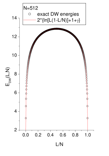
Figure 1: The excess energy of a DW positioned at the $L$th site of a chain with $N=512$, in units of $J$. The points represent exact values according to (24), the continuous line is the approximation of neglecting the contribution of $f(L)$ (cf. text).

IV.3 The DW’s entropy: analytical approximation

Neglecting the contribution of the $f$-term (cf. previous subsection), it is possible to write down an approximate partition function

$$Z_{DW}^{*}=e^{-2(\gamma+1)K}\sum_{j=1}^{N-1}\left\{\frac{1}{j(1-j/N)}\right\}^{2K}\quad,$$ (26)

where $K=J/T$. Three cases can be distinguished:

1. high temperatures, $K<1/2$: the sum in (26) can be approximated by an integral, where $j/N$ is substituted by a continuous variable:

   $$Z_{DW}^{*}=e^{-2(\gamma+1)K}N^{1-2K}\int_{0}^{1}dx\left\{\frac{1}{x(1-x)}\right\}^{2K}\quad;$$ (27)

   in this case the DW free energy is given by

   $$F_{DW}=-\frac{1-2K}{K}\ln N+O(N^{0}).$$ (28)

   DW formation can proceed spontaneously; the change in free energy is of order $-\ln N$.

2. $K=1/2$:

   $$Z_{DW}^{*} = e^{-(\gamma+1)}\sum_{j=1}^{N-1}\frac{1}{j(1-j/N)}$$ (29)

   $$= e^{-(\gamma+1)}\sum_{j=1}^{N-1}\left\{\frac{1}{j}+\frac{1}{N-j}\right\}$$

   $$= 2e^{-(\gamma+1)}\sum_{j=1}^{N-1}\frac{1}{j}$$

   $$= 2e^{-(\gamma+1)}\ln N+O(1/N)\quad.$$

   DW formation can still proceed spontaneously, with a free energy change of order $-\ln\ln N$.

3. $K>1/2$: The leading term in the first half ($j<N/2)$ of the discrete sum (26) - which is all that matters in the thermodynamic limit - can be obtained by neglecting the second factor in the denominator. Since the terms are symmetric around $j=N/2$, I estimate

   $$Z_{DW}^{*}\approx e^{-2(\gamma+1)K}\>2\zeta(2K)\quad.$$ (30)

   Note that in this case $Z_{DW}^{*}$ -and the DW free energy $-\ln Z_{DW}^{*}/K$ are of order $N^{0}$. Spontaneous DW formation occurs according to whether or not $Z_{DW}^{*}<1$. The critical temperature $T^{*}$ is obtained from the condition $Z_{DW}^{*}=1$, i.e.

   $$\frac{\ln 2\zeta(2K^{*})}{2K^{*}}=1+\gamma\quad.$$ (31)

   Numerical solution of (31) gives a value $K^{*}=0.65136$. Note that the value is quite close to the Anderson-Yuwal AnYu estimate $K_{c}=0.635$. In fact, for $K^{*}$ not too far from $1/2$, it is possible to use the limiting form of the $\zeta$ function $\zeta(2x)\approx 1/(2x-1)$; in this case (31) becomes

   $$-\frac{\ln(K^{*}-1/2)}{2K^{*}}=1+\gamma\quad.$$ (32)

   which is exactly the condition of AnYu .

IV.4 The DW entropy: numerical calculations

It is possible to use the exact expression (24) of the DW energy and calculate the partition function (4) numerically. The resulting DW free energy as a function of $K$ for a range of chain sizes is shown in Fig. 2. Note the different form of $N$-scaling for in the low and high $K$ regimes, cf. (28) and (30).

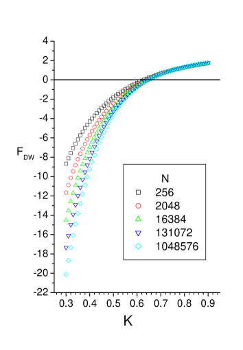
Figure 2: The numerically calculated free energy of a DW in units of $J$. as a function of the coupling constant $K$. Note the different form of $N$-scaling for in the low and high $K$ regime (cf. (28) and (30)). The dotted line marks the zero.

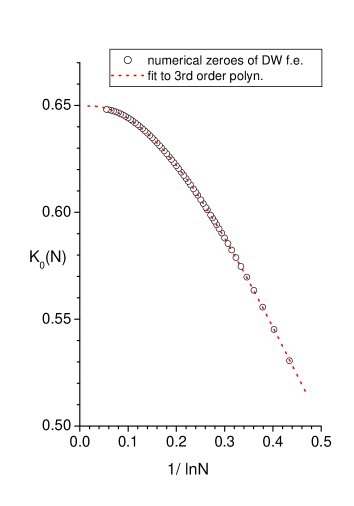
Figure 3: The zeroes of the numerically calculated DW free energy plotted as a function of $1/\ln N$. The continuous line is a fit of the type (33) and yields $K^{*}=0.6492(2)$.

The critical point is defined by the zero of the DW excess free energy (intersection of each curve with the dotted line in Fig. 2.) A third-order polynomial fit of zeroes obtained for sizes $10<N<8\times 10^{7}$, i.e.

$$K_{0}(N)=K^{*}+\frac{a_{1}}{\ln N}+\frac{a_{2}}{(\ln N)^{2}}+\frac{a_{3}}{(\ln N)^{3}}$$ (33)

(cf. Fig. 3) yields the estimate $K^{*}=0.6492(2)$ in the thermodynamic limit.

V Conclusions

I have reviewed recent work on one-dimensional lattice models with asymmetric on-site potentials, which are known to exhibit thermodynamic instabilities, i.e. transitions from a bound to an unbound state, at a temperature $T_{c}$. Such nonlinear models generically admit exact, unbounded solutions which can be regarded as domain walls. Examination of DW thermodynamics shows that a DW becomes entropically stable (i.e. the energy cost of producing it is balanced by the entropic gain) at a temperature $T^{*}$. In the case treated analytically, $T^{*}=T_{c}$; in the case treated numerically, equality holds within less than $1\%$.

A similar procedure was successfully applied to the one-dimensional ferromagnetic $S=1/2$ Ising model with inverse square interactions. In that case, the DW thermodynamics leads to a $T^{*}$ which also differs by less than $1\%$ from the best available numerical estimate of the critical temperature.

In summary, it appears that the vanishing of the DW free energy might be used as a “positive”criterion for the occurrence of a phase transition in one-dimensional systems, and at the same time provide an estimate of the critical temperature. In this sense, one might be tempted to conclude that phase transitions in one dimensional systems are indeed driven by DW formation.

References

- (1) L. van Hove, Physica 16, 137 (1950).
- (2) L. D. Landau and E. M. Lifshitz, Statistical Physics, Pergamon Press (1980).
- (3) Analyticity-based proofs of non-existence of phase transtions have recently been critically reviewed and generalized by J.A. Cuesta and A. Sanchez, J. Stat. Phys. 115, 869 (2004).
- (4) M. Peyrard and A.R. Bishop, Phys. Rev. Lett. 62, 2755 (1989).
- (5) D.J. Thouless, Phys. Rev. 187, 732 (1969).
- (6) E. Luijten and H. Meßingfeld, Phys. Rev. Lett. 86, 5305 (2001).
- (7) S. Aubry, J. Chem. Phys. 62, 3217 (1975).
- (8) S. Aubry, J. Chem. Phys. 64, 3392 (1976).
- (9) J. A. Krumhansl and J. R. Schrieffer, Phys. Rev. B11, 3535 (1975).
- (10) D. M. Kroll and R. Lipowski, Phys. Rev. B28, 5273 (1983); R. Lipowski, Phys. Rev. B32, 1731 (1985).
- (11) G. Parisi, Statistical Field Theory, Perseus (1998), page 221.
- (12) Y-L Zhang, W-M Zheng, J-X Liu, Y. Z. Chen, Phys. Rev. E 56, 7100 (1997).
- (13) N. Theodorakopoulos, Phys. Rev. E 68, 026109 (2003).
- (14) T. Dauxois, N. Theodorakopoulos and M. Peyrard, J. Stat. Phys. 107, 869 (2002).
- (15) N. Theodorakopoulos, M. Peyrard and R.S. MacKay, Phys. Rev. Lett. 93, 258101(2004).
- (16) P. W. Anderson and G. Yuval, J. Phys. C 4, 607 (1971).
- (17) The theoretical developments spanning over three decades are nicely reviewed by E.Luijten and H.W. J. Blöte, Phys. Rev. B56, 8945(1997).
- (18) E. Luijten, in Computer Simulation Studies in Condensed-Matter Physics XII, pp. 86-99, edited by D.P. Landau, S.P. Lewis and H.B. Schüttler (Springer, Heidelberg, 2000).